


ABSTRACT
We have studied the unusual time variability of an ultraluminous X-ray source in M 101, 4XMM J140314.2 + 541806 (henceforth, J1403), using Chandra and XMM-Newton data. Over the last two decades, J1403 has shown short-duration outbursts with an X-ray luminosity ∼1–3 × 1039 erg s−1, and longer intervals at luminosities ∼0.5–1 × 1038 erg s−1. The bimodal behaviour and fast outburst evolution (sometimes only a few days) are more consistent with an accretor/propeller scenario for a neutron star than with the canonical outburst cycles of stellar-mass black holes. If this scenario is correct, the luminosities in the accretor and propeller states suggest a fast spin (P ≈ 5 ms) and a low surface magnetic field (B ∼ 1010 G), despite our identification of J1403 as a high-mass X-ray binary. The most striking property of J1403 is the presence of strong ∼600-s quasi-periodic oscillations (QPOs), mostly around frequencies of ≈1.3–1.8 mHz, found at several epochs during the ultraluminous regime. We illustrate the properties of such QPOs, in particular their frequency and amplitude changes between and within observations, with a variety of techniques (Fast Fourier Transforms, Lomb–Scargle periodograms, weighted wavelet Z-transform analysis). The QPO frequency range <10 mHz is an almost unexplored regime in X-ray binaries and ultraluminous X-ray sources. We compare our findings with the (few) examples of very low frequency variability found in other accreting sources, and discuss possible explanations (Lense–Thirring precession of the inner flow or outflow; radiation pressure limit-cycle instability; marginally stable He burning on the neutron star surface).
1 INTRODUCTION
Short-term time variability in luminous X-ray binaries (in particular those that at some point reach or exceed their Eddington luminosity) is still largely unexplained or unexplored. We cannot assume that we have already discovered all possible types of time variability from the well-studied but limited sample of X-ray binaries in the Milky Way and Local Group. X-ray population studies in nearby galaxies have revealed the existence of entire classes of (rare) sources not present or not yet observed in the Milky Way: for example super-Eddington neutron stars (NSs), usually referred to as pulsar ultraluminous X-ray sources (PULXs), that reach luminosities ∼1040–1041 erg s−1 (Bachetti et al. 2014; Israel et al. 2017b, a; Sathyaprakash et al. 2019), or supersoft ULXs with characteristic temperatures ∼0.1 keV and luminosities of a few 1039 erg s−1 (Urquhart & Soria 2016). Thus, it is not surprising to discover also new variability behaviours.
Even the nearest galaxies outside the Local Group have been observed only a handful of times by Chandra and XMM-Newton: this hinders the study of state transitions and duty cycles and the search for X-ray eclipses; in addition, the low count rate usually limits the study of short-term variability and quasi-periodic oscillations (QPOs). Among the nearest large galaxies with an abundant population of X-ray binaries, M 101 (median Cepheid distance of 6.9 Mpc, from the NASA Extragalactic Database) is one of the targets with the largest number of archival observations (about 30 between Chandra and XMM-Newton) and is therefore one of the best places to look for such investigations.
One of the X-ray sources with the highest peak luminous in M 101, 2CXO J140314.3+541806 (Evans et al. 2019, 2010) = 4XMM J140314.2 + 541806 (Traulsen et al. 2020; Webb et al. 2020), henceforth, J1403 (Fig. 1), is an obvious candidate for such studies. Although previously recognized as a transient ULX (Heida et al. 2014; Wang et al. 2016; López et al. 2020), J1403 has received little attention so far in terms of individual X-ray studies. Simple flux estimates from a long sequence of Chandra and XMM-Newton observations between 2000 and 2017 (Section 2.1 for details) show that J1403 was in the ULX regime at LX ∼ a few 1039 erg s−1 some of the times, and was barely detected at LX ∼ a few 1037 erg s−1 on other occasions. Furthermore, we noticed that its short-term variability properties are even more remarkable than its state transitions. In this study, we will illustrate the presence of strong quasi-periodic oscillations (QPOs) on a characteristic time-scale of ∼600 s (∼1.7 mHz) in several of the epochs in which J1403 was in the ultraluminous regime.
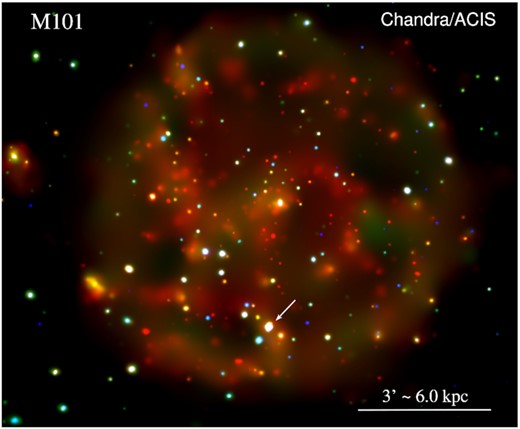
True-colour X-ray image of M 101, obtained by aligning and stacking all the available Chandra/ACIS observations of this galaxy. Colours are: red for 0.3–1 keV; green for 1–2 keV; blue for 2–7 keV. The individual colour images were adaptively smoothed with the ciao task csmooth. North is up, east is to the left. The target of our study, J1403, is marked with a small white arrow.
The origin of so-called very-low-frequency QPOs in X-ray binaries and in particular in ULXs is still unexplained, with several alternative possibilities (see Ingram & Motta 2019 for a review). Milli-Hz frequencies are too low to be consistent with Keplerian rotation from the region responsible for the X-ray emission (inner part of the accretion disc and/or hot spots on the surface of the NS). Instead, they might be associated with the Lense–Thirring precession of the inner disc (Motta et al. 2018), or of the outflow (Middleton et al. 2018). An alternative explanation for milli-Hz QPOs is repeated episodes of marginally steady He burning on the surface of the NS in low-mass X-ray binaries (Heger, Cumming & Woosley 2007a; Tse et al. 2021); however, such oscillations are expected to have a characteristic frequency ∼10 milli-Hz, and indeed the frequencies observed in the most promising candidates are ∼3–15 mHz (Tse et al. 2021). Some NS high mass X-ray binaries exhibit milli-Hz QPOs, too, but typically at frequencies ≳10 mHz (James et al. 2010). So far, only two NS high mass X-ray binaries have shown QPOs with similar frequencies to J1403. In LMC X-4, a QPO with a frequency varying between ≈0.65–1.35 mHz was seen (Moon & Eikenberry 2001) in correspondence of high-luminosity (likely super-Eddington) flares; this was interpreted as beating between the spin frequency of the NS and the Keplerian frequency of accreting clumps near the corotation radius. In IGR J19140 + 0951, a 1.46-mHz QPO was detected by Sidoli et al. (2016); they suggested that it could be produced by large-scale convective motion of a hot shell of gas that accumulates just outside the magnetospheric radius (‘settling accretion model’; Shakura et al. 2012). However, IGR J19140 + 0951 was in a low-luminosity state (LX ∼ 1034 erg s−1), much different from the ULX regime of J1403.
In this paper, we present the observational results of our study of J1403, based on the Chandra and XMM-Newton data analysis. We show how the source switches between high and low states, and discuss whether its luminosity evolution is more consistent with canonical outbursts of stellar-mass black holes (BHs; Fender, Belloni & Gallo 2004; Remillard & McClintock 2006; Fender & Muñoz-Darias 2016) or with accretor/propeller transitions in NSs and PULXs (Corbet 1996; Campana et al. 2002; Tsygankov et al. 2016; Campana et al. 2018). We use a variety of techniques to show that the QPOs are significant and to measure their frequencies. In particular, we use wavelet decomposition to build dynamical power spectra and show how the oscillating components change in amplitude and frequency during individual observations. We also derive the spin period and magnetic field that the NS in J1403 would have if the accretion/propeller scenario is applicable. We place those estimates in the context of younger and older NS populations. Finally, we refine the astrometric position and identify the optical counterpart in Hubble Space Telescope images.
2 DATA ANALYSIS
2.1 Chandra X-Ray Observatory
M 101 has been observed 28 times with Chandra X-Ray Observatory’s Advanced CCD Imaging Spectrometer (ACIS). The observation log is listed in Table 1; note that the ObsID numbering bears little relation to the actual time sequence. We downloaded the data from the public archives, then reprocessed and analysed them with the Chandra Interactive Analysis of Observations (ciao) software version 4.12 (Fruscione et al. 2006), Calibration Database 4.9.1. New level-2 event files and aspect solution files were created with the ciao tasks chandra_repro, followed by reproject_obs. We inspected each image with ds9 (Joye 2019) and used srcflux to identify those in which J1403 was significantly detected at the 90 per cent confidence level (using the Bayesian statistics of Kraft; Burrows & Nousek 1991). We found it in 26 observations. We used dmextract to build background-subtracted light curves (time resolution of 3.24 s). When there were sufficient counts for spectral analysis, we extracted spectra and associated response and ancillary response files with specextract (with the options ‘weight = no’ and ‘correctpsf = yes’, for point-like sources). For each srcflux, dmextract, and specextract analysis, we defined a source region with suitable size and shape, depending on the properties of the point spread function at that location for that particular observation. For example, for on-axis observations of the source, the extraction circle had a radius of 2.5 arcsec. Instead, for epochs in which the source was located several arcmin off-axis, at the edge of the S3 chip, we used a 5 × 7 arcsec source ellipse. Local background regions were at least four-times the size of the source regions.
Log of the Chandra observations.
| ObsID | Observation epocha | Exp. time | Count rateb |
|---|---|---|---|
| (ks) | (10−3 ct s−1) | ||
| 934 | 2000-03-26 00:20:55 | 98.38 | |$1.6^{+0.3}_{-0.2}$| |
| 2065 | 2000-10-29 08:05:35 | 9.63 | |$1.5^{+0.8}_{-0.6}$| |
| 4731 | 2004-01-19 05:57:05 | 56.24 | |$1.6^{+0.4}_{-0.4}$| |
| 5296 | 2004-01-21 10:57:22 | 3.09 | |$5.1^{+2.8}_{-2.0}$| |
| 5297 | 2004-01-24 01:34:02 | 21.69 | |$18.1^{+1.6}_{-1.6}$| |
| 5300 | 2004-03-07 09:29:06 | 52.09 | <0.2 |
| 5309 | 2004-03-14 01:41:21 | 70.77 | |$54.3^{+1.5}_{-1.5}$| |
| 4732 | 2004-03-19 08:15:25 | 69.79 | |$54.9^{+1.5}_{-1.5}$| |
| 5322 | 2004-05-03 07:44:34 | 64.70 | |$0.1^{+0.1}_{-0.1}$| |
| 4733 | 2004-05-07 13:29:38 | 24.81 | |$0.7^{+0.4}_{-0.3}$| |
| 5323 | 2004-05-09 03:11:31 | 42.62 | |$0.3^{+0.2}_{-0.2}$| |
| 5337 | 2004-07-05 18:42:37 | 9.94 | <0.5 |
| 5338 | 2004-07-06 13:27:55 | 28.57 | |$0.4^{+0.2}_{-0.2}$| |
| 5339 | 2004-07-07 13:24:00 | 14.32 | |$0.2^{+0.3}_{-0.2}$| |
| 5340 | 2004-07-08 11:07:26 | 54.42 | |$0.6^{+0.2}_{-0.1}$| |
| 4734 | 2004-07-11 01:43:17 | 35.48 | |$0.3^{+0.2}_{-0.1}$| |
| 6114 | 2004-09-05 18:23:48 | 66.20 | |$0.9^{+0.2}_{-0.2}$| |
| 6115 | 2004-09-08 18:16:36 | 35.76 | |$0.8^{+0.3}_{-0.3}$| |
| 6118 | 2004-09-11 15:15:08 | 11.46 | |$0.4^{+0.5}_{-0.3}$| |
| 4735 | 2004-09-12 12:59:30 | 28.78 | |$0.4^{+0.3}_{-0.2}$| |
| 4736 | 2004-11-01 18:43:08 | 77.35 | |$0.4^{+0.2}_{-0.1}$| |
| 6152 | 2004-11-07 07:03:53 | 44.09 | |$0.5^{+0.2}_{-0.2}$| |
| 6170 | 2004-12-22 01:17:57 | 47.95 | |$22.3^{+1.2}_{-1.2}$| |
| 6175 | 2004-12-24 16:38:17 | 40.66 | |$43.1^{+1.8}_{-1.9}$| |
| 6169 | 2004-12-30 02:10:50 | 29.38 | |$32.4^{+1.8}_{-1.8}$| |
| 4737 | 2005-01-01 14:30:53 | 21.85 | |$14.5^{+1.4}_{-1.4}$| |
| 14341 | 2011-08-27 10:37:29 | 49.09 | |$0.4^{+0.1}_{-0.2}$| |
| 19304 | 2017-11-08 20:42:03 | 36.57 | |$0.1^{+0.2}_{-0.1}$| |
a: time at the start of the observation;
b: net ACIS-S3 count rate in the 0.5–7 keV band, computed with srcflux, with an aperture correction to infinity. It is the observed rate, not corrected for the change in detector sensitivity over the years.
2.2 XMM-Newton
M 101 has been observed with XMM-Newton four-times. Publicly available European Photon Imaging Camera (EPIC) observations were downloaded from the High Energy Astrophysics Science Archive Research Center (HEASARC) data archive. We only used two observations (0104260101 and 0164560701: Table 2), because in the other two observations, the target ULX either fell on a chip gap or was off the field of view. The data were reduced using standard tasks within the Science Analysis System (sas) version 18.0.0. Intervals of strong background flaring were filtered out. The source was extracted using a circular region with a radius of 16 arcsec for 0104260101 and 13 arcsec for 0164560701; the local background was at least three times larger than the source regions. The small size of the source extraction circles was due to the locations of chip gaps and the need to avoid contamination from nearby (variable) point-like sources which are detected in the Chandra images. We used the standard flagging criteria of #XMMEA_EP plus FLAG = 0 for the pn camera and #XMMEA_EM for the MOS1 and MOS2 cameras. Additionally, we selected patterns 0–4 and 0–12 for pn and MOS, respectively. The task xmmselect was used to extract individual spectra and corresponding response and ancillary response functions for pn, MOS1, and MOS2. The individual spectra were inspected to verify consistency before being combined into a single EPIC spectrum using the epicspeccombine task. For our timing analysis, we first performed barycentric corrections using the sas task barycen. Next, pn, MOS1, and MOS2 background-subtracted light curves were created with the sas tasks evselect and epiclccorr before finally combining them into a single EPIC light curve using (the ftools package lcmath; Blackburn 1995). The time resolution of the EPIC light curve is 2.6 s.
Log of the XMM-Newton observations used in this work.
| ObsID | Observation epocha | Exp. time | Count rateb |
|---|---|---|---|
| (ks) | (10−3 ct s−1) | ||
| 0104260101 | 2002-06-04 02:06:57 | 42.3 | 90 ± 2 (pn)c |
| 42 ± 1 (MOS)c | |||
| 0164560701 | 2004-07-23 08:51:10 | 32.5 | 44 ± 1 (pn)d |
| 21 ± 1 (MOS)d |
| ObsID | Observation epocha | Exp. time | Count rateb |
|---|---|---|---|
| (ks) | (10−3 ct s−1) | ||
| 0104260101 | 2002-06-04 02:06:57 | 42.3 | 90 ± 2 (pn)c |
| 42 ± 1 (MOS)c | |||
| 0164560701 | 2004-07-23 08:51:10 | 32.5 | 44 ± 1 (pn)d |
| 21 ± 1 (MOS)d |
a: time at the start of the observation;
b: net EPIC pn and MOS1+MOS2 count rate in the 0.3–12 keV band, in the source extraction circle (no aperture correction or vignetting correction);
c: within a source extraction circle of 16 arcsec radius;
d: within a source extraction circle of 13 arcsec radius.
2.3 X-ray spectral analysis
We used xspec version 12.11.1 (Arnaud 1996) to perform the spectral fitting, over the 0.3–10 keV range for the XMM-Newton spectra and the 0.3–7 keV range for Chandra spectra. The two combined XMM-Newton/EPIC spectra, and seven Chandra/ACIS spectra (ObsIDs 4732, 4737, 5297, 5309, 6169, 6170, 6175) with ≳300 counts, were grouped to a minimum of 20 counts per bin so that we could use Gaussian statistics. Another seven Chandra/ACIS spectra (ObsIDs 934, 2065, 4731, 5296, 5340, 6114, 6115) have enough counts for a simple power-law fitting with the Cash statistics (Cash 1979), for which the data were rebinned to 1 count per bin. The absorbed and de-absorbed fluxes of those 16 observations were computed with the cflux task in xspec. The remaining 14 Chandra observations do not have enough counts for xspec fitting: the fluxes of J1403 in those data sets were estimated directly from the filtered event files, with the ciao task srcflux (Table 1).
2.4 X-ray time-frequency analysis
Firstly, we did a preliminary timing analysis with basic ftools tasks such as lcurve and powspec to inspect the data. Then, we used the Lomb–Scargle method to identify possible significant QPO peaks. The Lomb–Scargle periodogram (Lomb 1976; Scargle 1982) is a commonly used statistical tool designed to detect periodic signals in unevenly spaced observations. We calculated the Lomb–Scargle periodograms and their corresponding false alarm probabilities based on an implementation of astropy (Astropy Collaboration 2013, 2018). We did so for the two XMM-Newton observations and the seven Chandra observations with higher signal-to-noise (ObsIDs 4732, 4737, 5297, 5309, 6169, 6170, 6175).
In order to look for possible variations of a QPO frequency within individual observations, we also computed dynamical power spectra with the weighted wavelet Z-transform (WWZ) technique (Foster 1996). For this, we used libwwz,1 which is a python package based on the Fortran code of Foster (1996) and Templeton (2004), as well as on Aydin (2017)’s python 2.7 WWZ library. WWZs are widely used in many areas (e.g. Pulsar timing analysis by Lyne et al. 2010; supermassive black hole binary search by Graham et al. 2015; time-frequency analysis for light curve of dwarf nova by Ghaderpour & Ghaderpour 2020). As with other time-frequency analysis methods, there is a trade-off between time resolution and frequency resolution, which is controlled by a decay constant c. In our work, we followed Foster (1996) and chose c = 1/8π2 ≈ 0.0127. Thus the e-folding time (defined as the distance when the wavelet power falls to 1/e2, and it can be seen as the window width) is |$\sqrt{2} P$|. In our case, the QPO period is around 600 s, the corresponding e-folding time is 848 s, which is sufficient for period determination. In Fourier space, the full width at half-maximum (FWHM) of the frequency peak at 1/600 Hz is about |$2 \times 10^{-4}\, \mathrm{Hz}$|, lower frequency has smaller FWHM. Therefore, both the time resolution and frequency resolution is appropriate for our analysis.
Finally, after determining the most significant QPO frequencies at different times within each observation, we folded the light curves on those frequencies and obtained their phaseograms. We did that with the stingray (Huppenkothen et al. 2019a,b; Bachetti et al. 2021) python package, designed for spectral-timing analysis of X-ray data.
2.5 X-ray/optical astrometry
Using the Mikulski Archive for Space Telescopes, we selected and downloaded Hubble Space Telescope (HST) observations of M 101 that included the field of J1403. We found that this region was observed with the Advanced Camera for Surveys/Wide Field Camera (ACS/WFC) on 2002 November 13 (part of Program 9490); and with the Wide Field Camera 3/Ultraviolet and VISible light (WFC3/UVIS) imager on 2014 February 2 (Program 13364), and 2016 September 24 (Program 14166). We used 20 common sources in Gaia Early Data Release 3 (Gaia Collaboration 2016,2021) to verify and re-align the HST astrometry in every filter to better than ≈0.01 arcsec. We did not find enough unambiguous Chandra/HST point-like associations in the region around J1403 for a direct astrometric alignment between the two sets of images. However, the large number of Chandra observations enabled us to take an average value of the X-ray position with a smaller uncertainty than the typical astrometric error of individual observations. More specifically, we selected 16 Chandra observations where J1403 has a high number of counts and is not too far off-axis. In each of them, the position of J1403 was determined with the ciao task wavdetect, and the associated error (statistical uncertainty due to the centroiding algorithm) was computed with equation (5) from Hong et al. (2005); this error was then added in quadrature with a 1σ absolute astrometry uncertainty of ≈0.8 arcsec. The final X-ray position is a weighted average and its error is the weighted standard deviation. We obtained R.A. =14h03m14s.295, Dec. =+54°18′06|${_{.}^{\prime\prime}}$|26 with an uncertainty radius of ≈0.24 arcsec, which enabled us to pinpoint a likely optical counterpart in the HST images (Section 3.4).
3 RESULTS
3.1 Transient behaviour
The first motivation for our study was to characterize the outburst behaviour of this transient ULX. The long-term 0.3–10 keV light curve (Fig. 2) was obtained with a combination of measurements. For the 16 observations (14 from Chandra and two from XMM-Newton) with a sufficient number of counts, unabsorbed luminosities are the result of our xspec modelling (explained in more details in Section 3.3), with 90 per cent confidence limits computed with the cflux pseudo-model component. For the other 14 observations, the luminosities or upper limits plotted in Fig. 2 come from srcflux, under the assumption of a line-of-sight Galactic column density NH = 9 × 1020 cm−2 (Kalberla et al. 2005; HI4PI Collaboration 2016), a power-law photon index Γ = 1.7 (which is a representative value for the low state of Galactic black holes: e.g., Chakrabarti & Titarchuk 1995; Shaposhnikov & Titarchuk 2006; Sobolewska et al. 2011; Yang et al. 2015), and a proper calculation of the local auxiliary response function (srcflux parameter ‘point spread function method = arfcorr’). srcflux was applied over the 0.5–7 keV band, but we extrapolated the flux values to the 0.3–10 keV band, for consistency. We stress that we do not have enough counts to determine whether the spectra of the fainter group of observations ( LX ≲ 1038 erg s−1) is really a power law or is also dominated by thermal emission in the soft band; a power law is just the simplest approximation. If the soft X-ray emission is thermal even in the fainter epochs, the estimated unabsorbed 0.3–10 keV luminosity would be about 25 per cent lower than estimated with a power-law model.
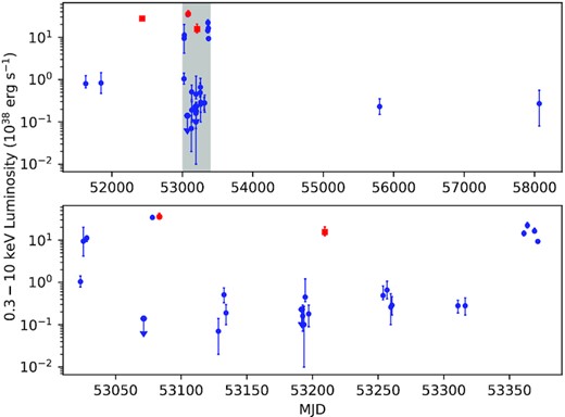
Long-term light curve derived from 28 Chandra observations (circles) and two XMM-Newton observations (squares). The datapoints represent the average unabsorbed 0.3–10 keV luminosity during each observation. Such values were obtained from xspec spectral modelling whenever possible (as explained in Section 2.3) or with srcflux for the observations with few counts. Red data points indicate observations in which strong QPOs are detected (in chronological order: ObsIDs 0104260101, 4732, 0164560701). The grey-shaded time interval in the upper panel is displayed zoomed-in in the lower panel.
In most cases, J1403 was found at an X-ray luminosity between a few × 1037 erg s−1 and ≈1 × 1038 erg s−1. There were five separate flaring episodes to a luminosity ≳ 1039 erg s−1 recorded over a 17-yr timeline (i.e., five epochs at ULX level separated by at least one detection at a lower luminosity). There is no evidence of a regular pattern for the outbursts. Transitions from lower to upper luminosities occur sometimes on short time-scales: a change from LX ≈ 1038 erg s−1 to LX ≈ 1039 erg s−1 happened over only 2 d, in 2003 January. By 2003 March, the X-ray source had declined below a detection limit of ≈1037 erg s−1, but a week later it was up again as a ULX at LX ≈ 3 × 1039 erg s−1. On at least a couple of epochs, namely Chandra during ObsIDs 4737 (Fig. A1) and 6170 (Fig. A5), luminosity changes by an order of magnitude occurred on time-scales ≲ 104 s. We will discuss the intra-observational variability in more details in Section 3.2. Interestingly, J1403 appears to spend very little time in the luminosity range between ≈1038 erg s−1 and ≈1039 erg s−1, which is where transient stellar-mass BHs spend the majority of their time in outburst (Fender & Muñoz-Darias 2016).
3.2 Short-term variability and QPOs
The intra-observation variability of J1403 proved to be also unusual. It is immediately clear from visual inspection (Fig. 3) that light curves from the two XMM-Newton observations contain a markedly regular pattern (particularly ObsID 0164560701). We computed power density spectra of the two light curves with the ftools task powspec (fast Fourier transform algorithm). They show significant peaks at characteristic frequencies just above ∼1 mHz (Figs 4 and 5). Then, we inspected the power density spectra of the Chandra observations extracted using powspec, and found a significant peak at ∼1.632 mHz in at least one observation, ObsID 4732 (Fig. 6), corresponding to the highest luminosity recorded by Chandra (LX ≈ 3.6 × 1039 erg s−1).
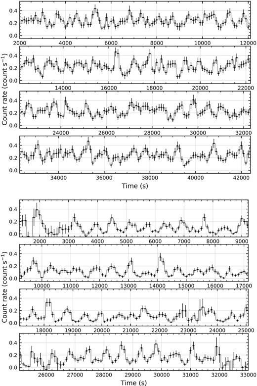
XMM-Newton/EPIC background-subtracted light curves from the observations in 2002 (top; ObsID 010426101) and 2004 (bottom; ObsID 0164560701), binned to 100 s.
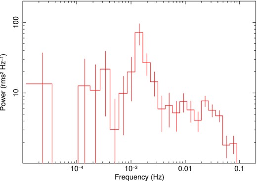
Power spectral density of J1403 derived from the XMM-Newton/EPIC light curve from observation 0104260101. The white noise level has been subtracted (parameter ‘norm = −2’ in powspec).

As in Fig. 4, for the XMM-Newton/EPIC light curve from observation 164560701.
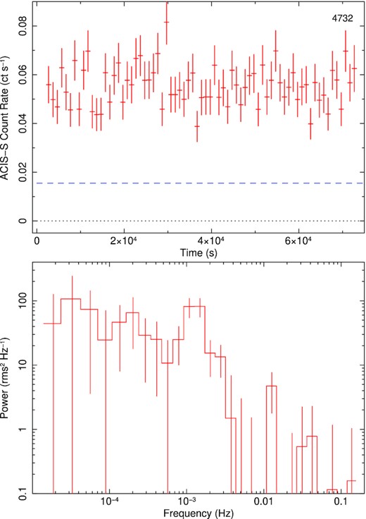
Top panel: Light curve of Chandra ObsID 4732. The dashed line represents the count rate corresponding to an approximate de-absorbed 0.3–10 keV luminosity of 1039 erg s−1 (based on our detailed spectral modelling). Bottom panel: Power spectral density from the same observation, computed with powspec, after white noise subtraction.
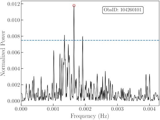
Lomb–Scargle periodogram of XMM-Newton ObsID 104260101. The open red circle indicates the most significant frequency, and the dashed blue line shows the 1 per cent false alarm probability level.
We used the Lomb–Scargle analysis to quantify the significant frequencies more precisely. We found significant QPO frequencies (false alarm probability level <1 per cent, which is estimated with the method of Baluev 2008) in the three observations already mentioned above (XMM-Newton ObsIDs 0104260101 and 0164560701, Chandra ObsID 4732); they are summarized in Table 3 and displayed in Figs 7, 8, and 9. In all three cases, the strongest oscillations have characteristic periods of ∼600 s. In the rest of this paper, we will focus on the analysis of those three observations. Several other Chandra observations show candidate QPO frequencies (usually also in the range of ∼1.5–2.5 mHz: Table 3), although they do not reach the 1 per cent false alarm probability threshold as in ObsID 4732. In most of those cases, the power of frequencies are higher than the short sub-intervals of the observations in which a QPO is present (as we shall illustrate with the dynamical power spectra). A summary of Lomb–Scargle results for a selection of bright Chandra observations is reported in Appendix A.
Main QPO frequencies and periods found with our WWZ analysis, in both XMM-Newton observations and in the Chandra observations with the highest signal-to-noise ratio.
| ObsID | Significant QPOs | Candidate QPOs |
|---|---|---|
| Chandra | ||
| 4732 | 1.632 mHz = 612.791 s | 1.003 mHz = 997.250 s |
| 1.308 mHz = 764.700 s | ||
| 4737 | 7.682 mHz = 130.183 s | |
| 1.368 mHz = 730.932 s | ||
| 3.153 mHz = 317.205 s | ||
| 5297 | 6.647 mHz = 150.440 s | |
| 2.688 mHz = 372.054 s | ||
| 1.892 mHz = 528.473 s | ||
| 5309 | 1.734 mHz = 576.724 s | |
| 1.583 mHz = 631.615 s | ||
| 6169 | 1.730 mHz = 578.031 s | |
| 21.099 mHz = 47.396 s | ||
| 1.548 mHz = 645.843 s | ||
| 2.948 mHz = 339.246 s | ||
| 1.912 mHz = 523.106 s | ||
| 6170 | 0.182 mHz = 5480.675 s | |
| 6175 | 1.595 mHz = 627.021 s | |
| 1.799 mHz = 555.885 s | ||
| XMM-Newton | ||
| 0104260101 | 1.645 mHz = 607.739 s | |
| 1.349 mHz = 741.208 s | ||
| 1.917 mHz = 521.635 s | ||
| 0164560701 | 1.734 mHz = 576.561 s | |
| 1.614 mHz = 619.422 s | ||
| 1.659 mHz = 602.910 s | ||
| 1.539 mHz = 649.938 s | ||
| 1.577 mHz = 634.314 s | ||
| 1.444 mHz = 692.588 s | ||
| 1.785 mHz = 560.239 s | ||
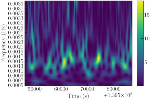
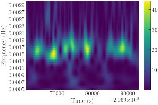
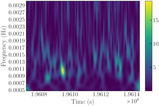
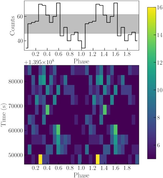
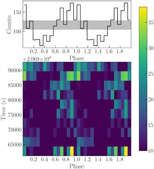
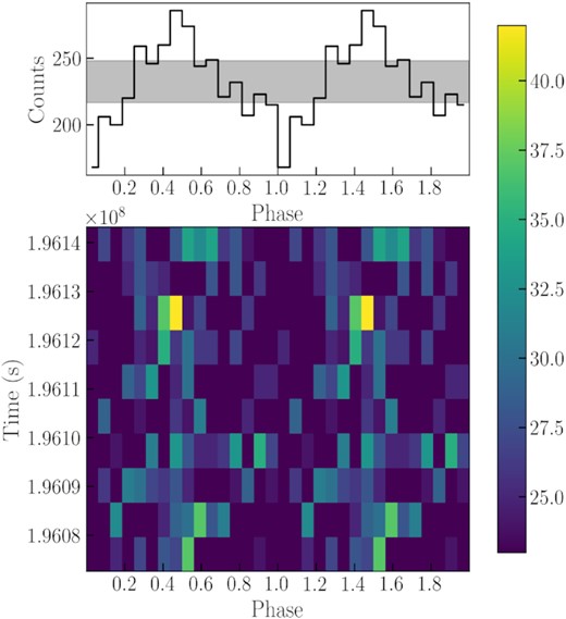
For the third step of our timing analysis, we used the WWZ technique, to look for intra-observational changes in the QPO frequencies and intensities. We found that the QPO appears and disappears within individual observations, and their frequencies also have some slight drifts (Figs 10, 11, and 12). We also studied whether the phase of the oscillation was preserved during individual observations (Figs 13, 14, and 15 show three examples of phaseograms). Their phases basically remain constant, although XMM-Newton ObsID 0104260701 shows a possible slow trend. However, we cannot confirm this trend because our long QPO period results in a low time resolution.
Finally, as an independent check, we searched for periodicities in the same three observations (XMM-Newton ObsIDs 0104260101 and 0164560701, Chandra ObsID 4732) with the ftools task efsearch, which works by folding the light curve over a range of test periods, and determining the χ2 of the folded light curves for each period. We then used the efold task to plot the light curves folded on to the most significant period. The results are consistent with those found from the Lomb–Scargle analysis. For the first and second XMM-Newton observations, we find best-fitting folding periods of (607.5 ± 1.0) s and (575.9 ± 1.0) s, respectively (Fig. 16 and 17). For the Chandra ObsID 4732, we find (612.8 ± 1.5) s. The folded light curves of the three observations are shown in Figs 16 and 18.
3.3 Spectral properties
All the X-ray spectra with sufficient signal-to-noise ratio (i.e., those corresponding to LX ≳ 1039 erg s−1) share a general property: they are mildly curved over the Chandra/XMM-Newton band. Thus, they cannot be fitted with a simple power law. Single thermal emission components (blackbody, standard disc, p-free disc) also do not provide a good fit, because they are more curved than the observed data. This is a common situation in ULXs. By analogy with previous spectral analysis in the literature (Walton et al. 2018), we fitted the spectra with a double thermal component (blackbody plus p-free disc: Tables 4 and 5, Figs 19, 20, and 21). The double-thermal model provides two characteristic temperatures and two associated radii. The higher temperature is typically ∼1.5–2 keV, for a blackbody emitting size ∼30–60 km. The lower temperature is ∼0.4–0.5 keV and corresponds to inner disc radii ∼200–400 km.
We also tried to fit the spectra with Comptonization models: for example simpl×diskbb, simpl×diskpbb, nthcomp, and diskir. Such models provide statistically equivalent results to the double thermal models. The two characteristic best-fitting temperatures in the Comptonization models are also around 1.5–2 keV and 0.4–0.5 keV. In this framework, the higher temperature corresponds to the energy of the Comptonizing electrons, and the lower temperature is associated with the seed disc photons. A more detailed comparison of the different spectral models is beyond the scope of this paper, which is more focused on the peculiar time variability properties.
In three of the Chandra observations (ObsIDs 4732, 5297, 5309), the spectral fits are significantly improved by the addition of a thermal plasma component around 1 keV. Such components are often seen in ULX spectra even at CCD resolution (Middleton et al. 2015) and are resolved into a complex structure of emission and absorption lines at grating resolution (Pinto, Middleton & Fabian 2016; Pinto et al. 2017; Kosec et al. 2018). They are interpreted as signatures of the super-Eddington outflow characteristic of ULXs, especially for accretion discs seen at high inclination (denser outflow along our line of sight). However, for J1403, there is no significant thermal plasma component in the two XMM-Newton observations, despite their higher signal-to-noise compared with the Chandra observations at similar luminosity. Thus, based on the available data, we cannot determine whether the outflow signatures are real and whether they are persistent or transient.
Another caveat is that the p index of the disc model component tends to the lowest limit (p = 0.5), both for double-thermal models (bb plus diskpbb) and for Comptonization models (simpl*diskpbb). This indicates that the spectral curvature of this component is mild, and significantly lower than that expected from a standard disc. Overall, the best-fitting components may be nothing more than phenomenological tools in xspec to reproduce a mildly curved spectrum.
3.4 Optical counterpart
We find a single bright optical point source within the 0.24 arcsec X-ray error circle (Fig. 22). The Vega magnitudes are listed in Table 6. At first glance, the colours and magnitudes appear consistent with typical optical counterparts of ULXs. We use the latest set of Padova stellar isochrones,2 with metallicity Z = 0.019, to estimate the physical characteristics of the companion star. Both the UVIS and ACS data suggest an age of ≈15 Myr, with a mass of ≈15 M⊙, a temperature of ≈15 000–25 000 K and a bolometric luminosity of ≈3 × 1038 erg s−1.
We also use the combined ACS-WFC and WFC3-UVIS data set to fit a simple de-reddened blackbody spectrum in xspec. The best-fitting model suggests that the emission is coming from a surface with a radius of |$\approx 34^{+38}_{-21}$| R⊙ at a temperature of |$\approx 16,800^{+8000}_{-4000}$| K and a luminosity of (3.1 ± 0.5) × 1038 erg s−1. This is in agreement with the kind of star expected from the isochrones results. We find a slight (factor of <1.2) excess in emission in the F814W band compared with the expected blackbody flux. This is likely to be due to contamination from at least one neighbouring (red) star, partially blended with the much brighter and bluer counterpart. We do not know what the X-ray luminosity was at the time of the optical observations. However, even if the X-ray source was at its peak levels of ∼3 × 1039 erg s−1, the contribution of an irradiated outer disc to the optical luminosity must be at least an order of magnitude lower than the intrinsic optical/UV luminosity of the donor star. In other words, the brightness of the optical counterpart suggests that J1403 is a high-mass X-ray binary.
Previous studies (Heida et al. 2014) had suggested a bright infrared source, consistent with a red supergiant, as the counterpart of J1403. In fact, follow-up HST observations showed four bright stars, potential optical candidates, within a 0.7 arcsec X-ray positional error circle (López et al. 2020): the red supergiant and three bluer sources. With our improved X-ray astrometric precision (error circle of 0.24 arcsec), we have ruled out the red supergiant and have identified instead as the true optical counterpart the bright blue star labelled ‘Source D’ in López et al. (2020).
4 DISCUSSION
4.1 Comparison with low-frequency QPOs in other systems
QPOs (see e.g. Ingram & Motta 2019 for a recent review) have been studied in stellar-mass BHs and NSs since their first discovery in low-mass X-ray binaries with NS accretors, in the early ’80s (Motch et al. 1983). Although there are open questions about the genesis of QPOs in both BH and NS binaries, their study has the potential to provide clues on the nature of the accretor, and even constrain its mass and spin. While being highly statistically significant, the QPOs detected in J1403 do not show any property that allows us to unambiguously classify them. Their most relevant characteristic is that they are detected at a frequency lower than that of the large majority of QPOs observed in Galactic accretors. Several QPO models have been proposed over the years (Ingram & Motta 2019), and some of them seem capable of producing QPO behaviour with characteristics consistent with those we find in J1403.
Let us assume first that the 600-s QPOs seen in J1403 are an extreme case of some previously known classes of low-frequency QPOs. Low-frequency QPOs in BH X-ray binaries are observed at frequencies ≳0.1 Hz. They are divided into three classes: Type A, Type B, and Type C (Casella, Belloni & Stella 2005 for e.g.). Such classes roughly correspond to three QPO classes observed in NS X-ray binaries (flaring branch, normal branch, and horizontal branch oscillations, respectively; see Motta et al. 2017). Type-C QPOs are the most common class of BH QPOs: they are seen in the low/hard state, hard-intermediate state, and high/soft state of BH transients (Belloni et al. 2005; Belloni 2010). Their centroid frequency increases with luminosity, starting from as low as ∼0.1 Hz in the low/hard state at the beginning and end of an outburst. Type-A and Type-B QPOs generally appear in the soft-intermediate state, at higher frequencies (around 5–7 Hz), and remain currently unexplained.
Lense–Thirring precession (Lense & Thirring 1918; Wilkins 1972), a relativistic frame-dragging effect expected to occur in the vicinity of a spinning compact mass, has been invoked as a possible explanation for Type-C QPOs (Stella & Vietri 1998; Ingram, Done & Fragile 2009; Ingram et al. 2016; Middleton et al. 2018). In particular, Ingram et al. (2009) proposed that Type-C QPOs are associated with a global, rigid precession of a misaligned, geometrically thick inner disc. Test-particle models of relativistic precession have also been considered and have been shown to be limiting cases of the global disc precession models (Motta et al. 2018). Although this effect is likely to occur in virtually all accreting NS and BH systems, we cannot directly relate it to the QPOs in J1403 as it would be difficult to explain the very low frequency of the QPO in this system. Such frequencies would require an extremely slowly spinning compact object (fig. 8 in Motta et al. 2018), or extreme values of the disc aspect ratio H/R, of the viscosity α, or of the surface density profile. Much lower Lense–Thirring precession frequencies (consistent with those in J1403) are predicted if the X-ray luminosity oscillations come from the photosphere of a precessing outflow, rather than the precessing inner disc (Middleton et al. 2019).

As in Fig. 7, for XMM-Newton ObsID 164560701. A zoomed-in inset of the significant frequencies are shown in the middle right. It shows that there is a series of significant lower-frequency harmonics of the strongest frequency.
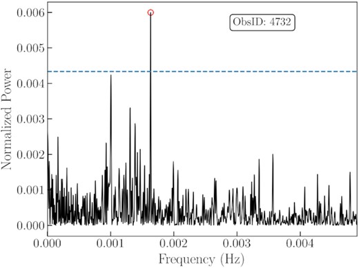
As in Fig. 7, for Chandra ObsID 4732.
WWZ dynamical power spectrum for XMM-Newton ObsID 104260101.
As in Fig. 10, for XMM-Newton ObsID 164560701.
As in Fig. 10, for Chandra ObsID 4732.
Phaseogram of XMM-Newton ObsID 104260101. The top panel shows the light curve folded by the 607.739-s period, which is the most significant frequency indicated in Fig. 7. The shaded grey area shows the mean Poisson confidence level. The bottom panel shows the phase variations during the observation.
As in Fig. 13, for XMM-Newton ObsID 164560701.
As in Fig. 13, for Chandra ObsID 4732.
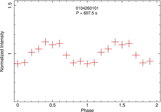
0.3–10 keV background-subtracted light curve of XMM-Newton ObsID 104260101, folded over a period of 607.5 s. This is the period that provides the best χ2 in the efsearch analysis; it is consistent (within the efsearch uncertainty) with the characteristic period of 607.7 s found with the Lomb–Scargle analysis.

0.3–10 keV background-subtracted light curve of XMM-Newton ObsID 164560701, folded over a period of 575.9 s (consistent with the strongest period of 576.6 s found with the Lomb–Scargle analysis).
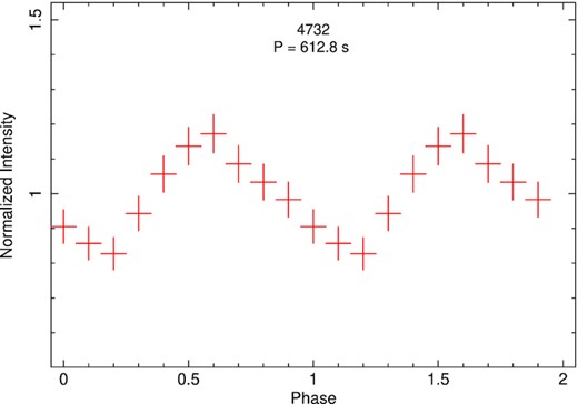
0.3–7 keV background-subtracted light curve of Chandra ObsID 4732, folded over a period of 612.8 s (identical to the period found with the Lomb–Scargle analysis).
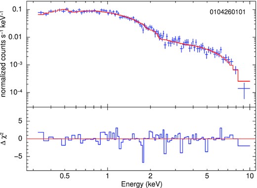
X-ray spectrum and model residuals from XMM-Newton ObsID 0104260101, fitted with tbabsGal × tbabs × (bbodyrad + diskpbb). The data sets from pn, MOS1, and MOS2 were combined with the sas task epicspeccombine and grouped to >20 counts per bin. The best-fitting parameter values are listed in Table 4.
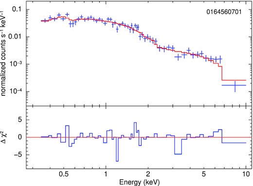
As in Fig. 19, for the spectrum from XMM-Newton ObsID 0164560701.
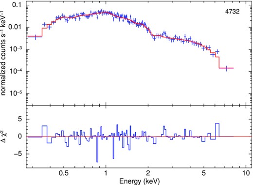
X-ray spectrum and model residuals from Chandra ObsID 4732, fitted with tbabsGal × tbabs × (bbodyrad + diskpbb). The data were grouped to >20 counts per bin. The best-fitting parameter values are listed in Table 5.
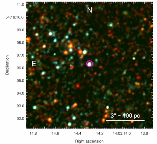
HST/ACS-WFC RGB image: Blue represents the F435W filter, green is F555W, and red is F814W. The 0.24 arcsec magenta region indicates the X-ray position of J1403. A bright blue optical source is coincident with the X-ray position, likely from a blue giant companion star, optical emission from the outer accretion disc, or a combination of the two.
The expected precession frequency in Lense–Thirring models is proportional to |$a\, r^{-3}$| where a is the spin parameter and r is either the spherization radius of the disc (in disc precession models) or the photosphere of the precessing outflow (Middleton et al. 2019). Given the observational uncertainties in both parameters, it is easy to find values of a and r that satisfy almost any observed frequency, from minutes to days, including the 600-s range seen in J1403. However, it is precisely the steep dependence on r that makes those models unsuitable to our case. The radius of the geometrically thick part of the precessing flow (spherization radius in super-critical accretion) scales with |$\dot{m}$| (Poutanen et al. 2007); the photospheric radius of the precessing outflow scales with |$\dot{m}^{3/2}$| (equation 13 in Middleton et al. 2019). So, we expect the Lense–Thirring precession frequency to have a strong dependence on |$\dot{m}$|. On the other hand, the luminosity in the ultraluminous regime is a much weaker function of |$\dot{m}$|: |$L \propto L_{\rm Edd} \, (1+\ln \dot{m})$| for BHs and weakly magnetized NSs (Poutanen et al. 2007), dominated by massive disc outflows at the spherization radius. Therefore, in the Lense–Thirring scenario, we expect that changes in the QPO frequency from epoch to epoch should be much larger than the corresponding luminosity changes, for a change of |$\dot{m}$|. This is not the case in J1403, where the strongest QPOs are detected within a small range of frequencies (≈1.5–1.7 mHz) despite changes in X-ray luminosity by factor of 3 between the corresponding epochs (years apart).
Next, we consider the possibility that the 1.6-mHz oscillations in J1403 are not related to BH Type-C QPOs. Instead, we look for alternative mechanisms of very-low-frequency variability in NSs. Some NS accretors exhibit QPOs at a range of frequencies from about 5–15 mHz (Revnivtsev et al. 2001), an order of magnitude lower than Type-C QPOs. It has been proposed that such QPOs are associated with the marginally stable nuclear burning of matter on the surface of the NS in an accretion regime near or an order of magnitude below the Eddington limit (Heger, Cumming & Woosley 2007b; Keek, Cyburt & Heger 2014; Mancuso et al. 2019; Tse et al. 2021). The ignition of matter in different regions of the NS surface produces a quasi-periodic modulation of the emission coming directly from the crust, observable as a QPO with a soft energy spectrum (Heger et al. 2007b). However, because accretion on to NSs produces more energy per unit mass than does nuclear burning, each burst (which is essentially Eddington-limited) provides only a small fraction of the energy produced by extraction of gravitational potential energy. This would make it difficult to identify the signature of marginally stable burning in a NS accretor located in galaxies as distant as M 101. Furthermore, theoretical work (Heger et al. 2007b) predicts that the QPOs arising from marginally stable burning would display frequencies a factor of a few larger than what observed in J1403. Thus, while we cannot exclude such an origin for the QPO in J1403, we lack circumstantial evidence further supporting such an interpretation.
A comparison with the very-low-frequency QPOs in the high mass X-ray binary LMC X-4 is perhaps more relevant for our system. LMC X-4 is powered by a NS with a spin period of ≈13.5 s, a binary period of 1.4 d, and a superorbital period of ≈30.5 d (e.g. Naik & Paul 2004; Falanga et al. 2015; Brumback et al. 2018). It is one of the few high-mass X-ray binaries fed via disc accretion rather than wind accretion (a possible similarity with ULX pulsars), from an ≈18 M⊙ companion filling its Roche lobe. LMC X-4 has a persistent X-ray luminosity of ∼1038, with occasional aperiodic flares peaking at ≈2 × 1039 erg s−1 (Moon, Eikenberry & Wasserman 2003). During the super-Eddington flares, very-low-frequency QPOs were detected in two frequency bands (≈0.65–1.35 mHz and ≈2–20 mHz; Moon & Eikenberry 2001), overlapping with the QPO frequencies in J1403. A possible scenario proposed for the lowest frequency band was the beating between the spin frequency of the NS and the Keplerian frequency of the disc at its inner radius (magnetospheric radius), which would extend a little inside the corotation radius during the flares.
Only a few other systems are known to produce quasi-periodic modulations at frequencies ∼1 mHz. These modulations may not always be strictly classified as QPOs, but are none the less characterized by a preferred frequency. Particularly noteworthy is the case of the BH X-ray binary GRS 1915 + 105, which is known to exhibit several different variability classes, some of which highly repetitive and with a period in the range of 10–1000 s (Belloni et al. 2000). Among these classes, the ρ class, sometimes referred to as the ‘heartbeats’, is the most regular (and arguably the most studied), and appears with a (mildly variable) period between ≈40 s and ∼1000 s. This type of variability has been identified in two additional Galactic X-ray binaries: a relatively low-luminosity BH X-ray binary, IGR J17091−3624 (Altamirano et al. 2011; Janiuk et al. 2015), and the NS X-ray binary MXB 1730−335 (also called the Rapid Burster, Bagnoli & in’t Zand 2015). A similar variability pattern has been observed in a ULX, 4XMM J111816.0−324910, with a characteristic time-scale of ≈3500 s (Motta et al. 2020), and in a number of active Galaxies (particularly noteworthy the case of GSN 069; Miniutti et al. 2019).
Because of its extreme brightness, the spectral and timing properties of GRS 1915 + 105 have been studied over the last three decades with every major X-ray telescope (the Rossi X-ray Timing Explorer, ASCA, Suzaku, XMM-Newton, Chandra, Nicer, etc.). The inner disc is radiation-dominated, the luminosity is around or slightly above the Eddington limit, and there is evidence of winds from the outer disc. Absorption lines associated with winds have been observed at the time of broadband spectral changes (Ueda, Yamaoka & Remillard 2009). The heartbeat quasi-periodic variability has been modelled as a limit-cycle behaviour associated with interactions between radiation and accreting matter at super-Eddington accretion rates (Done, Wardziński & Gierliński 2004; Neilsen, Remillard & Lee 2011; Neilsen, Petschek & Lee 2012). This model could in principle offer a possible explanation for the QPOs in J1403. However, as discussed in Motta et al. (2020) for the case of the ULX in 4XMM J111816.0−324910, the poor knowledge of the system itself makes it impossible to draw any firm conclusion on the matter.
Finally, among the extragalactic ULX class, M 74 X-1 (CXOU J013651.1 + 154547) has shown perhaps the most impressive example of intra-observational flaring, on time-scales of ≈5000 s ≈0.2 mHz (Krauss et al. 2005) in at least one Chandra observations (but not in others). There is currently no information on the nature of this compact object and of its donor star, and the nature of the above modulation remains unclear. Other examples of ULXs flaring on time-scales of ∼10 000 s are NGC 7456 ULX-1 (Pintore et al. 2020) and NGC 4559 X7 (Pintore et al. 2021). However, the flaring variability in those sources appears stochastic (possibly related to inhomogeneities in the super-critical disc outflow), without the quasi-periodic pattern so strongly detected in J1403.
4.2 Nature of the compact object
The X-ray spectral properties of J1403 do not give substantial clues about the nature of the accretor. A slightly curved 0.3–10 keV spectrum, consistent with a double thermal model or with Comptonization, is typical of ULXs (Walton et al. 2018) but does not discriminate between a NS and a BH accretor. Both classes of compact objects would be in the ultraluminous regime in the epochs when LX > 1039 erg s−1. As for the epochs in which LX < 1038 erg s−1, the lack of counts does not permit us to discriminate between NS and BH models. The general evolution of the flares, with the rapid rise from LX < 1038 erg s−1 to LX > 1039 erg s−1, and equally rapid declines, does not resemble the behaviour of BH transients (Tetarenko et al. 2018) in Galactic low-mass X-ray binaries, and is also very different from the few confirmed BHs in high-mass systems (Cyg X-1, LMC X-1, LMC X-3). Giant flares with peak X-ray luminosities sometimes in excess of 1039 erg s−1 are a feature of NSs in Be X-ray binaries (Martin et al. 2014), which are associated with moderately young stellar populations. Even in those cases, though, a smooth, gradual decline from peak luminosity is observed over several weeks, consistent with the viscous time-scale of the (transient) accretion disc (Lutovinov et al. 2017; Tsygankov et al. 2017; Wilson-Hodge et al. 2018; Vasilopoulos et al. 2020).
Perhaps the best clue to the nature of the compact object comes from the luminosity distribution of the various epochs. We have already noted (Fig. 2) that J1403 tends to be found at LX ≳ 1039 erg s−1 or at LX ≲ 1038 erg s−1, but more rarely in between. In the top panel of Fig. 23, we replotted the same average de-absorbed luminosities of all 30 observations as a histogram over the luminosity range. From that, we confirm the presence of a scarcely populated gap of about an order of magnitude in luminosity. If J1403 is an ordinary stellar-mass black hole, the luminosity gap corresponds to the typical high/soft state range, a state in which other black hole transients typically spend several weeks during each complete outburst (Remillard & McClintock 2006; Fender & Muñoz-Darias 2016). A small caveat for the estimate of the gap size is that the luminosities below the gap have been estimated with a power-law model, while those above the gap with double-thermal model. As we noted in Section 3.3, if the spectra below the gap are also thermal, their luminosity would be about 25 per cent lower and the gap correspondingly larger.
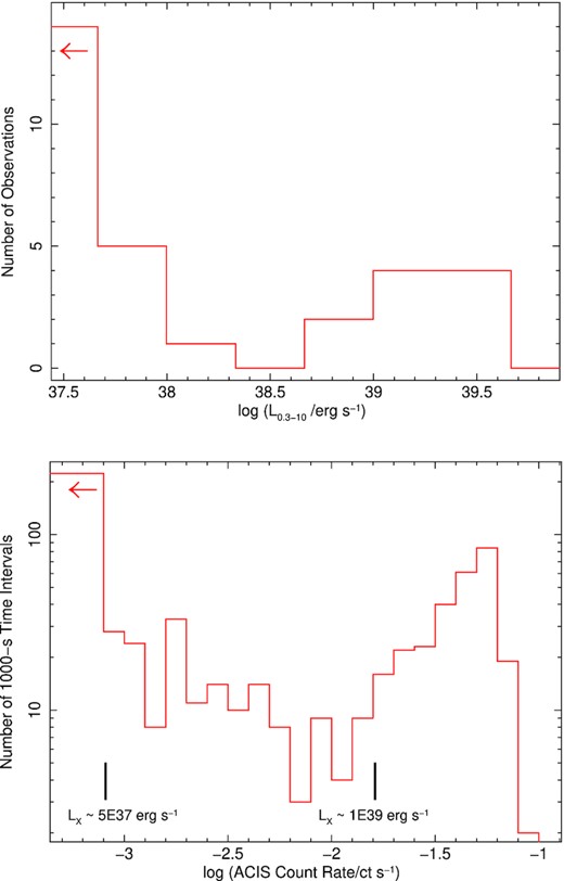
Top panel: Distribution of the average 0.3–10 keV de-absorbed luminosities of all the 28 Chandra observations and two XMM-Newton observations. (The first bin on the left corresponds to observations with LX < 4.6 × 1037 erg s−1.) Bottom panel: Distribution of 0.3–7 keV background-subtracted ACIS count rates in 1000-s intervals, for the 14 Chandra observations with higher luminosity. Two black markers identify the approximate count rates corresponding to 0.3–10 keV de-absorbed luminosities of 5 × 1037 erg s−1 and 1 × 1039 erg s−1. To account for the decline in sensitivity of the ACIS detector, the observed count rates were rescaled to ‘equivalent’ Cycle-5 count rates, with pimms. (The first histogram bin on the left corresponds to the number of 1000-s intervals with no detected net counts.).
To obtain an alternative estimate of the gap, we took the Chandra background-subtracted light curves from the 14 observations with higher signal-to-noise ratio (the same ones listed in Table 4), and rebinned them to 1000 s. The histogram of the count rate distribution (in log scale) is plotted in the bottom panel of Fig. 23. This time, the approximate luminosity conversion is based on the best-fitting spectral model for ObsID 4732 for all bins. The lowest portion of the distribution (bins with <20 occurrences) is between net ACIS-S rates (converted to equivalent Cycle 5 rates with pimms) of ≈1.6 × 10⁻³ ct s−1 and ≈1.6 × 10⁻² ct s−1.
Spectral parameters for the XMM-Newton/EPIC observations, fitted with tbabsGal × tbabs × (bbodyrad + diskpbb). Uncertainties are the 90 per cent confidence limits for one interesting parameter.
| Parameter | Value in each ObsID | |
|---|---|---|
| 0104260101 | 0164560701 | |
| |$N_{\rm {H,Gal}}^a$| | [0.09] | [0.09] |
| |$N_{\rm {H,int}}^a$| | <0.01 | <0.02 |
| |$kT_{\rm {bb}}^b$| | |$1.69^{+0.26}_{-0.16}$| | |$1.62^{+0.41}_{-0.21}$| |
| |$N_{\rm {bb}}^c$| | |$2.7^{+1.1}_{-0.8} \times 10^{-3}$| | |$1.6^{+1.2}_{-0.7} \times 10^{-3}$| |
| |$kT_{\rm {in}}^d$| | |$0.50^{+0.06}_{-0.03}$| | |$0.49^{+0.08}_{-0.07}$| |
| p | <0.52 | <0.53 |
| |$N_{\rm {dpbb}}^e$| | |$6.1^{+5.5}_{-1.9} \times 10^{-2}$| | |$3.6^{+4.8}_{-1.8} \times 10^{-2}$| |
| |$\chi ^2_{\nu }$| | 0.98 (87.3/89) | 1.16 (58.2/50) |
| |$F_{0.3-10}^f$| | |$38.7^{+2.0}_{-2.0}$| | |$18.7^{+1.5}_{-1.4}$| |
| |$L_{0.3-10}^g$| | |$27.8^{+1.2}_{-1.2}$| | |$13.5^{+0.9}_{-0.9}$| |
a: Units of 1022 cm−2.
b: Temperature of the blackbody component (bbodyrad); units of keV.
c: Nbb = (Rbb/d10)2, where Rbb is the blackbody radius (units of km), and d10 the distance to the galaxy (units of 10 kpc; here, d10 = 680).
d: Peak temperature of the slim disc component (diskpbb); units of keV.
e: Ndpbb = (rin/d10)2cos θ, where rin is the ‘apparent’ inner radius of the disc (units of km), d10 the distance to the galaxy (units of 10 kpc; here, d10 = 680), and θ is our viewing angle.
f: Observed flux in the 0.3–10 keV band; units of 10−14 erg cm−2 s−1.
g: De-absorbed luminosity in the 0.3–10 keV band, defined as 4πd2 times the de-absorbed model flux; units of 1038 erg s−1.
Spectral properties in selected Chandra/ACIS observations. The seven spectra with >300 counts were grouped to a minimum of 20 counts per bin, and fitted with tbabsGal × tbabs × (apec + bbodyrad + diskpbb), with the χ2 statistics. The other seven spectra were grouped to 1 count per bin, and fitted with tbabsGal × tbabs × power law, with the Cash statistics. Uncertainties are the 90 per cent confidence limits for one interesting parameter.
| Parameter | Value in each ObsID | |||||||||||||
|---|---|---|---|---|---|---|---|---|---|---|---|---|---|---|
| 934 | 2065 | 4731 | 4732 | 4737 | 5296 | 5297 | 5309 | 5340 | 6114 | 6115 | 6169 | 6170 | 6175 | |
| |$N_{\rm {H,Gal}}^a$| | [0.09] | [0.09] | [0.09] | [0.09] | [0.09] | [0.09] | [0.09] | [0.09] | [0.09] | [0.09] | [0.09] | [0.09] | [0.09] | [0.09] |
| |$N_{\rm {H,int}}^a$| | <0.13 | <0.37 | <0.12 | <0.02 | <0.09 | <0.12 | <0.09 | <0.01 | <0.23 | <0.09 | <0.27 | <0.07 | <0.04 | <0.07 |
| |$kT_{\rm {apec}}^b$| | – | – | – | |$1.19^{+0.19}_{-0.16}$| | – | – | |$0.68^{+0.20}_{-0.36}$| | |$1.75^{+2.50}_{-0.54}$| | – | – | – | – | – | – |
| |$N_{\rm {apec}}^c$| | – | – | – | |$1.3^{+0.7}_{-0.6}$| | – | – | |$0.49^{+0.28}_{-0.29}$| | |$2.2^{+7.8}_{-1.5}$| | – | – | – | – | – | – |
| |$kT_{\rm {bb}}^d$| | – | – | – | |$1.45^{+0.26}_{-0.16}$| | |$0.73^{+0.27}_{-0.14}$| | – | |$1.54^{+1.65}_{-0.54}$| | |$1.65^{+0.47}_{-0.21}$| | – | – | – | |$1.00^{+0.32}_{-0.15}$| | |$1.80^{+1.00}_{-0.40}$| | |$1.43^{+0.69}_{-0.33}$| |
| |$N_{\rm {bb}}^e\, \left(10^{-3}\right)$| | – | – | – | |$6.2^{+3.4}_{-2.4}$| | |$25^{+34}_{-20}$| | – | |$2.0^{+5.8}_{-1.6}$| | |$3.8^{+2.5}_{-2.0}$| | – | – | – | |$11.5^{+8.4}_{-8.2}$| | |$1.7^{+2.7}_{-1.1}$| | |$3.7^{+5.2}_{-2.5}$| |
| |$kT_{\rm {in}}^f$| | – | – | – | |$0.45^{+0.07}_{-0.07}$| | |$0.23^{+0.14}_{-0.07}$| | – | |$0.36^{+0.27}_{-0.13}$| | |$0.49^{+0.10}_{-0.10}$| | – | – | – | |$0.34^{+0.09}_{-0.10}$| | |$0.48^{+0.16}_{-0.12}$| | |$0.41^{+0.11}_{-0.07}$| |
| p | – | – | – | <0.54 | [0.5] | – | [0.5] | <0.52 | – | – | – | <0.8 | <0.59 | <0.64 |
| |$N_{\rm {dpbb}}^g$| | – | – | – | |$0.10^{+0.19}_{-0.04}$| | |$0.9^{+7.5}_{-0.8}$| | – | |$0.08^{+0.44}_{-0.07}$| | |$0.07^{+0.11}_{-0.04}$| | – | – | – | |$0.24^{+3.15}_{-0.16}$| | |$0.03^{+0.16}_{-0.02}$| | |$0.16^{+0.78}_{-0.11}$| |
| |$\Gamma _{\rm {pl}}^h$| | |$2.49^{+0.58}_{-0.36}$| | |$1.9^{+2.4}_{-0.7}$| | |$1.40^{+0.35}_{-0.34}$| | – | |$2.23^{+0.25}_{-0.23}$| | |$0.85^{+0.83}_{-0.80}$| | – | – | |$1.64^{+1.18}_{-0.47}$| | |$2.65^{+0.77}_{-0.50}$| | |$1.29^{+0.73}_{-0.53}$| | – | – | – |
| |$N_{\rm {pl}}^i$| | |$3.0^{+1.3}_{-0.6}$| | |$2.5^{+6.5}_{-1.0}$| | |$2.0^{+0.6}_{-0.5}$| | – | |$33.1^{+4.0}_{-3.7}$| | |$8.7^{+7.5}_{-4.9}$| | – | – | |$1.6^{+1.9}_{-0.4}$| | |$1.8^{+0.7}_{-0.4}$| | |$1.1^{+1.2}_{-0.4}$| | – | – | – |
| |$\chi ^2_{\nu }$| | – | – | – | 0.95 (112.6/118) | 1.06 (10.6/10) | – | 1.04 (12.5/12) | 0.77 (94.5/123) | – | – | – | 1.04 (36.4/35) | 0.65 (25.3/39) | 1.15 (63.0/55) |
| C-stat/dof | 0.88 (87.0/99) | 1.43(17.11/12) | 0.71 (49.1/69) | – | – | 2.1 (22.9/11) | – | – | 0.84 (38.8/46) | 0.92 (54.9/50) | 0.83 (23.3/28) | – | – | – |
| |$F_{0.3-10}^j$| | |$0.89^{+0.22}_{-0.18}$| | |$1.2^{+1.2}_{-0.7}$| | |$1.71^{+0.70}_{-0.49}$| | |$47.4^{+2.6}_{-3.1}$| | |$11.8^{+1.9}_{-1.8}$| | |$15.2^{+20.8}_{-8.5}$| | |$16.5^{+7.4}_{-4.4}$| | |$48.3^{+2.1}_{-3.3}$| | |$0.58^{+0.21}_{-0.20}$| | |$0.56^{+0.20}_{-0.14}$| | |$1.10^{+0.76}_{-0.46}$| | |$22.3^{+2.6}_{-2.2}$| | |$23.2^{+5.5}_{-4.9}$| | |$29.5^{+5.0}_{-3.3}$| |
| |$L_{0.3-10}^k$| | |$0.80^{+0.44}_{-0.16}$| | |$0.83^{+0.63}_{-0.36}$| | |$1.04^{+0.38}_{-0.26}$| | |$33.5^{+2.0}_{-1.9}$| | |$9.5^{+4.7}_{-1.3}$| | |$9.4^{+10.7}_{-5.2}$| | |$11.2^{+4.0}_{-2.4}$| | |$34.0^{+2.5}_{-2.1}$| | |$0.45^{+0.76}_{-0.10}$| | |$0.49^{+0.33}_{-0.10}$| | |$0.66^{+0.41}_{-0.25}$| | |$17.1^{+1.6}_{-0.9}$| | |$15.6^{+2.9}_{-2.2}$| | |$24.5^{+3.2}_{-4.1}$| |
a: Units of 1022 cm−2.
b: Units of keV.
c: Units of |$10^{-19}/\lbrace 4\pi d^2\rbrace \, \int n_en_{\rm H} \, dV$|, where d is the luminosity distance in cm, and ne and nH are the electron and H densities in cm−3.
d: Temperature of the blackbody component (bbodyrad); units of keV.
e: Nbb = (Rbb/d10)2, where Rbb is the blackbody radius (units of km), and d10 the distance to the galaxy (units of 10 kpc; here, d10 = 680).
f: Peak temperature of the slim disc component (diskpbb); units of keV.
g: Ndpbb = (rin/d10)2cos θ, where rin is the ‘apparent’ inner radius of the disc (units of km), d10 the distance to the galaxy (units of 10 kpc; here, d10 = 680), and θ is our viewing angle.
h: Power-law photon index (for spectra with a low number of counts).
i: Power-law normalization; units of 10−6 photons keV−1 cm−2 s−1 at 1 keV.
j: Observed flux in the 0.3–10 keV band; units of 10−14 erg cm−2 s−1.
k: De-absorbed luminosity in the 0.3–10 keV band, defined as 4πd2 times the de-absorbed model flux; units of 1038 erg s−1.
Apparent brightness of the optical counterpart (Vegamag system), measured from the HST observations.
| Obs. date | Filter | ||||
|---|---|---|---|---|---|
| F275 | F336 | F435/438 | F555 | F814 | |
| 2002-11-13a | 22.9 ± 0.1 | 22.9 ± 0.1 | 22.7 ± 0.1 | ||
| 2014-02-15b | 21.3 ± 0.1 | 21.5 ± 0.1 | |||
| 2016-09-24b | 22.8 ± 0.1 | 22.8 ± 0.1 | |||
| Obs. date | Filter | ||||
|---|---|---|---|---|---|
| F275 | F336 | F435/438 | F555 | F814 | |
| 2002-11-13a | 22.9 ± 0.1 | 22.9 ± 0.1 | 22.7 ± 0.1 | ||
| 2014-02-15b | 21.3 ± 0.1 | 21.5 ± 0.1 | |||
| 2016-09-24b | 22.8 ± 0.1 | 22.8 ± 0.1 | |||
aACS/WFC
bWFC3/UVIS
A possible interpretation of this bimodal distribution is that J1403 is a NS that switches between accretor and propeller states (Illarionov & Sunyaev 1975; Ghosh & Lamb 1979) between observations – or even within individual observations, as suggested by the rapid count rate evolution for example during Chandra ObsIDs 4737 (Fig. A1) and 6170 (Fig. A5). In the rest of Section 4.2, we will assume this is the case. We will explore the consequences of this assumption for other system parameters, to determine whether it is at least a physical scenario (without claiming it should be the only possible one).
The assumption of radiative efficiency in the accretor state is because of the hard surface of the neutron star; in the propeller state, because the luminosity is just below Eddington, at a level usually characterized by a standard disc. The factor of 2 in the ratio of the radii (often forgotten in the literature) is because surface accretion releases an amount of energy |$\propto M\dot{M}/R$| while an accretion disc radiates only an energy |$\propto M\dot{M}/2R$|.
For the observed ratio Lacc/Lprop ≈ 10, equation (1) suggests a spin period |$P \approx 5\, M_{1.4}^{-1/2}$| ms. Even if we relax the definition of luminosity gap by a factor of 2, the period is still ≲15 ms.
Typical magnetic fields in NS high-mass X-ray binaries are between 1012–1013 G (Pan et al. 2018; van den Eijnden et al. 2021). There is at least one well-known example of a luminous (at times, super-Eddington) high-mass X-ray binary, SMC X-1, with B ≈ 1011 G, estimated from its spin-up rate (Li & van den Heuvel 1997), although a much higher field was recently proposed (B ≈ 4.2 × 10¹² G) if an X-ray feature at ≈55 keV is interpreted as a cyclotron line (Pradhan, Maitra & Paul 2020). However, there are no known examples of high-mass X-ray binaries with a spin frequency as high as ∼200 Hz and a surface field as low as ≈2 × 10¹⁰ G. The high spin frequency is more typical of low-mass X-ray binary, while the inferred field is intermediate between those measured in high- and low-mass systems (Mukherjee et al. 2015; van den Eijnden et al. 2021). We will comment on this issue further in Section 4.3.
Finally, we compare the magnetospheric radius (inner radius of the disc) with the spherization radius Rsph, to determine whether we expect strong outflows from the truncated disc, similar to what we expect from a super-critical disc around a black hole. Using again the model of radiation-pressure-dominated disc in Chashkina et al. (2017), the condition H/R ≈ 1 (standard definition of spherization radius) in the inner disc is reached for |$\dot{m} \approx 10$|, corresponding to L ≈ 2 × 1039 erg s−1 (note that the definition of |$\dot{m}$| in Chashkina et al. (2017) is different from our definition because we have included the efficiency factor η ≈ 0.2). We compare this estimate with the well-known derivation of |$R_{\rm {sph}}/R_{\rm in} \approx (5/3)\, \dot{m}$|, from Poutanen et al. (2007). The latter expression was derived for a black hole disc, and requires some adaptation for the case of a disc truncated at the magnetospheric radius. However, we can follow Poutanen et al. (2007) and adopt their definition of Rsph as the radius where the integrated disc luminosity L(R > Rsph) = LEdd (independent of the magnetospheric radius). For J1403, the bolometric disc luminosity in the propeller state is always below Eddington (up to L ≈ 1.5 × 1038 erg s−1 at the transition to accretor state). Thus, there is no spherization radius and probably no strong outflow in the propeller state. In the accretor state, we expect the disc component of the luminosity to become super-Eddington for L ≈ 2 × 1039 erg s−1 (|$\dot{m} \approx 10$|), in agreement with the estimate from Chashkina et al. (2017).
Recapping our argument, we have suggested that the two characteristic radii in J1403, when observed in the ultraluminous regime, are a magnetospheric radius at ∼30–50 km (inside the corotation radius and quite close to the NS surface, because of the low magnetic field) and a spherization radius located an order of magnitude further out (corresponding to |$\dot{m} \sim 10$|). It is an interesting coincidence that these two values are similar to the characteristic radii of the two thermal components used for our spectral modelling (Section 3.3). A common interpretation of the higher temperature component in pulsar ULXs (Walton et al. 2018) is that it comes from the geometrically thick portion of the (non-standard) disc between the spherization radius and the magnetospheric radius. An alternative interpretation (Koliopanos et al. 2017; Mushtukov et al. 2017) is that the hotter thermal emission comes mostly from accretion curtains at the magnetospheric radius, where the inflow gets deflected along the poloidal field lines out of the disc plane.
4.3 A NS spun up by accretion?
We noted earlier than the inferred fast spin and moderately low magnetic field are more typical of pulsars in low-mass rather than high-mass X-ray binaries, even though J1403 appears to belong to a young stellar population. Here we use a simple model to assess whether the pulsar evolution towards fast spin and low magnetic field could have been caused by the huge amount of accretion, on a time-scale consistent with the lifetime of a high-mass donor star.
In summary, if J1403 was constantly accreting in the super-Eddington regime, at a luminosity ∼1039 erg s−1, it may take only ∼105 yr to get spun up to a period of 5 ms and to have its magnetic field reduced from a ‘canonical’ initial value ∼1012 G to the current inferred value ∼1010 G. The NS would accrete a mass ∼0.1 M⊙ during this evolution. In fact, J1403 is only in the ULX state for ∼10 per cent of the time, and we may assume that the spin and surface field evolution in the propeller state is small compared with that in the accretor state. Thus, the age of the source is more likely ∼106 yr. In any case, it is a short time-scale, perfectly consistent with the lifetime of a massive donor star. If this scenario is correct, J1403’s evolution is very similar to the evolution proposed by Kluzniak & Lasota (2015) for the pulsar ULX M 82 X-2 (also a high-mass X-ray binary). The latter source has a spin period of 1.37 s but is spinning up (during its super-Eddington regime) at a fast rate |$\dot{P} \approx - 2 \times 10^{-10}$| s s−1 (Bachetti et al. 2014) and may become a millisecond pulsar in ∼105 yr (Kluzniak & Lasota 2015). J1403 may be a similar system, simply at a later stage of evolution, when the NS has already been spun up to a millisecond period.
5 CONCLUSIONS
The time variability behaviour of the high mass X-ray binary J1403 makes it difficult to classify it into previously known classes of accreting compact objects. Its optical counterpart is consistent with a young, massive donor star, with an age of ≈15 Myr and a mass of ≈15 M⊙. In most of the observations over a baseline of 17 yr, J1403 is detected at X-ray luminosities between a few × 1037 erg s−1 and ≈1038 erg s−1, typical for a wind-fed high mass X-ray binary. However, it has flared occasionally to luminosities of about 1–4 × 1039 erg s−1. The flaring episodes have short rise and decay times, much shorter than the viscous time-scale of a temporary accretion disc (as is the case for example for Type II bursts in a Be X-ray pulsar). In some observations, the transition between luminosities <1038 erg s−1 and >1039 erg s−1 occurred in less than 104 s. A magnetospheric gate provides a mechanism for sharp changes of luminosity. However, if the observed luminosity jumps are due to the accretor/propeller switch, the classical magnetospheric conditions (valid for a Keplerian disc coupled with a dipole field) imply a very fast spin (P ∼ 5–15 ms) and a low magnetic field (B ∼ 2–7 × 10¹⁰ G), unusual for a young pulsar. We speculated that the supercritical accretion rate is reducing the surface field, and, at the same time, spinning up the NS. Alternatively, the magnetic field has strong non-dipolar components, so that our simple disc truncation model is not valid. This is the case proposed for example for the transient super-Eddington pulsar SMC X-3 (Tsygankov et al. 2017) and for the ULX NGC 5907 X-1 (Israel et al. 2017b). Exploring this non-dipolar scenario is beyond the scope of this work.
The observational class of confirmed (from X-ray pulsations) pulsar ULXs does not contain millisecond pulsars yet. The shortest spin period in this class is ≈0.42 s for NGC 7793 P13 (Fürst et al. 2016; Israel et al. 2017a). All other pulsar ULXs have spin periods longer than 1 s (see a review table in Chen, Wang & Tong 2021). However, the fast spin-up rate in some of those ULXs suggests that they may evolve to become millisecond pulsars on time-scales shorter than the lifetime of the super-Eddington accretion phase (Kluzniak & Lasota 2015). We propose that J1403 is one example of this evolution process. So, why have we not detected any millisecond pulsar ULXs yet? We suggest that it is an observational bias. X-ray pulsations have been detected so far only in the brightest sources, with ≳10 000 detected counts per observation. In order to detect pulsations on a millisecond time-scales from ULXs in external galaxies, we need at the same time high count rate, good spatial resolution (or an isolated source), and millisecond time resolution. Only XMM-Newton/EPIC-pn in timing mode can provide enough sensitivity and time resolution, but at the expense of spatial resolution. Only two bright, isolated ULXs (Holmberg II X-1 and Holmberg IX X-1) have been significantly tested for millisecond pulsations, without a detection (Israel, private communications).
Regardless of the nature of the compact object, what makes J1403 truly remarkable is the presence of strong QPOs, at frequencies variable from epoch to epoch, but generally in the range of ≈1.3–1.8 mHz. Very little is known about the physical origin of such very-low-frequency variability in X-ray binaries in general, let alone in ULXs. We reviewed several alternative scenarios proposed to explain low-frequency variability in other luminous X-ray binaries: Lense–Thirring precession of the inner disc or of a disc outflow; nuclear burning on the surface of the NS; ‘heartbeat’ limit-cycle instability; beat frequency between material rotating at the inner edge of the Keplerian disc and the NS surface. There is no strong evidence in favour of any one of those scenarios. Exploration of new theoretical scenarios is left to further work.
ACKNOWLEDGEMENTS
We thank Manfred Pakull for his comments and suggestions. This research is based on data obtained from the Chandra Data Archive and has made use of software provided by the Chandra X-ray Center (CXC) in the application package ciao. We also used data obtained from the ESA’s XMM-Newton Science Archive (XSA), and data from the NASA/ESA Hubble Space Telescope. The latter are associated with programs 9490, 13364, and 14166, and were obtained from the Space Telescope Science Institute, which is operated by the Association of Universities for Research in Astronomy, Inc., under NASA contract NAS 5-26555. To analyse some of the data, we used the galaxy (https://github.com/sammarth-k/galaXy) software and its data products. We also used the VizieR catalogue access tool, CDS, Strasbourg, France (DOI : 10.26093/cds/vizier). The original description of the VizieR service was published in 2000, A&AS 143, 23.
RTU acknowledges support from the Packard Foundation. RS acknowledges grant number 12073029 from the National Science Foundation of China. PE and GLI acknowledge financial support from the Italian Ministry for Education and Research through the PRIN grant 2017LJ39LM. SEM acknowledges financial contribution from the agreement ASI-INAF n.2017-14-H.0, the INAF mainstream grant, and the PRIN-INAF 2019 n.15.
DATA AVAILABILITY
All data are public and retrievable from the XMM-Newton, Chandra data archives, and from the Mikulski Archive for Space Telescopes (for HST).
Footnotes
REFERENCES
APPENDIX A: SPECTRAL AND TIMING PROPERTIES OF SELECTED OTHER CHANDRA OBSERVATIONS
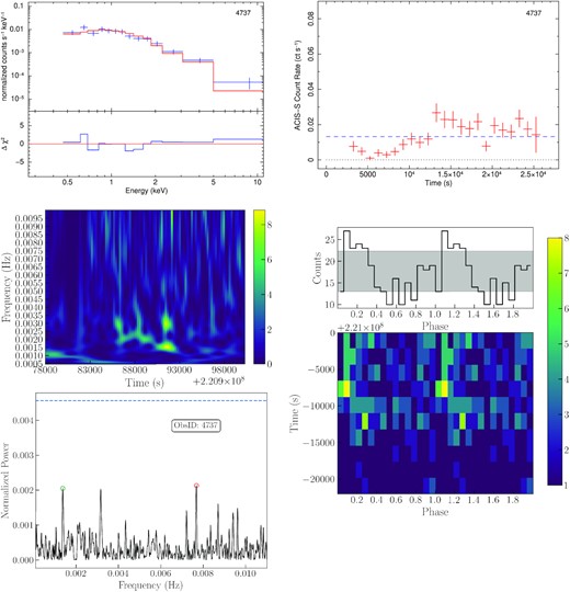
Summary of the main spectral and timing properties of J1403 during Chandra ObsID 4737. Left column, top panel: X-ray spectrum fitted with an absorbed double-thermal model (bbodyrad + diskpbb in xspec), and corresponding χ2 residuals (see Table 4 for the fit parameters, flux, and luminosity). Right column, top panel: background-subtracted count rate in the 0.5–7 keV band (binned to 1000 s). The dashed blue line corresponds to an approximate unabsorbed 0.3–10 keV luminosity of 1039 erg s−1, based on the best-fitting spectral model. Left column, middle panel: WWZ dynamical power spectrum, showing a strong QPO over a short interval of the observation. Left column, bottom panel: Lomb–Scargle analysis of the most significant frequencies. The dashed blue line represents a 99 per cent significance level over the whole observation. The open red circle is the most significant frequency and the green circle indicates a local peak around the 1.5 mHz. Right column, bottom panel: Phaseogram and folded light curve with using local frequency peak indicated by the open green circle.


