


ABSTRACT
Efforts are underway to use high-precision timing of pulsars in order to detect low-frequency gravitational waves. A limit to this technique is the timing noise generated by dispersion in the plasma along the line of sight to the pulsar, including the solar wind. The effects due to the solar wind vary with time, influenced by the change in solar activity on different time-scales, ranging up to ∼11 yr for a solar cycle. The solar wind contribution depends strongly on the angle between the pulsar line of sight and the solar disc, and is a dominant effect at small separations. Although solar wind models to mitigate these effects do exist, they do not account for all the effects of the solar wind and its temporal changes. Since low-frequency pulsar observations are most sensitive to these dispersive delays, they are most suited to test the efficacy of these models and identify alternative approaches. Here, we investigate the efficacy of some solar wind models commonly used in pulsar timing using long-term, high-cadence data on six pulsars taken with the Long Wavelength Array, and compare them with an operational solar wind model. Our results show that stationary models of the solar wind correction are insufficient to achieve the timing noise desired by pulsar timing experiments, and we need to use non-stationary models, which are informed by other solar wind observations, to obtain accurate timing residuals.
1 INTRODUCTION
Pulsars are rapidly rotating and highly magnetized neutron stars (Hewish et al. 1968), which produce beamed broad-band emission, due to relativistic effects near the neutron star, and are most commonly observed at radio frequencies. This emission appears as a pulsed signal due to the very stable rotation periods of neutron stars, producing a pulse that is only a fraction of a period in width when the cone of emission from the pulsar sweeps across the line of sight (LoS) to the observer. Even though individual pulses from a pulsar vary, the average pulse profile is generally stable in frequency over time-scales of years to decades (Helfand, Manchester & Taylor 1975; Liu et al. 2012). This unique property of pulsars allows them to serve as precision clocks, where the arrival time of a subsequent pulse can be predicted to high accuracy.
Among the population of pulsars, millisecond pulsars (MSPs; see e.g. Backer et al. 1982) are a sub-class that are believed to be older pulsars, which are ‘recycled’ by accreting material from a companion and thereby have been spun up to millisecond rotational periods. MSPs can provide precision in the period measurement of one part in 1013 or better, compared to one part in 107 for a normal pulsar (see e.g. Lorimer 2008). This makes them useful for a range of projects such as tests of general relativity, navigation, etc., via pulsar timing experiments (see e.g. Manchester 2017). Perhaps the most interesting among these is the long-term monitoring of a set of high-precision pulsars to detect gravitational waves from supermassive blackhole binaries in the nanohertz regime (e.g. Demorest et al. 2013). These experiments are generally referred to as pulsar timing arrays (PTAs), with the North American Nanohertz Observatory for Gravitational Waves (Alam et al. 2021), European Pulsar Timing Array (Chen et al. 2021), and Parkes Pulsar Timing Array (Abbott et al. 2018) being three major efforts in this direction.
Since the DM contribution from the ionosphere is of the order of 10−5 pc cm−3, it is much smaller than the current sensitivities of PTAs, and hence we do not address the ionospheric contribution in this paper. The next significant contribution to DM variations comes from the SW. This is of the order of 10−3 to 10−4 pc cm−3, depending on the solar elongation of the pulsar, and so needs to be accounted for (see e.g. Tiburzi et al. 2021). Most pulsar timing analysis packages use a simple spherical model of the SW. The SW itself is composed of slow dense streams and faster, more diffuse streams, and it is necessary to understand the mix of such structures along the LoS to the pulsar in order to make the appropriate corrections. Additionally, there are transient phenomena called coronal mass ejections (CMEs) associated with eruptions on the Sun, which are harder to model but contribute significantly to the SW DM (see e.g. Shaifullah, Tiburzi & Zucca 2020; Krishnakumar et al. 2021). Temporal variations on many different time-scales also occur in the SW due to solar activity: time-scales of days (active region evolution), the solar rotation period (27 d), and the solar cycle (∼11 yr). As mentioned before, solar elongation plays a critical role in the size of the correction needed due to the much higher densities occurring close to the Sun.
The largest contribution to the variation can arise from fluctuations in the IISM, which can be of the order of 10−3 pc cm−3. Previous studies have shown significant change over periods of a few days to weeks (e.g. Backer et al. 1993); Hobbs et al. (2004) proposed the relation |$|\rm {d(DM)}/{d\mathit{ t}}| \approx 0.0002 \sqrt{DM}$| pc cm−3 yr−1, relative to typical DM values of tens of pc cm−3. The DM fluctuations arise mainly due to relative motion of spatial structures in the IISM that occur along the LoS to the pulsar. The IISM can have small-scale structures that drive fluctuations (see e.g. Bansal et al. 2020). Finally, at times it can be difficult to disentangle the effects due to the SW and the IISM (see e.g. Tiburzi et al. 2019), which makes it difficult to create a model applicable in all situations.
In this paper, we use long-term regular monitoring observations of pulsars with the Long Wavelength Array (LWA) at frequencies below 88 MHz, along with data from several higher cadence solar campaigns, to study DM fluctuations due to the SW and IISM and assess the efficacy of existing SW models for PTA experiments, including comparison with a non-stationary model of the SW. Section 2 describes the observational and data acquisition set-up, and Section 3 describes the SW and relevant models evaluated. Section 4 describes the methods used to calculate the DM via pulsar timing, calculation of the SW contribution from models, and the modelling of the IISM contribution. Sections 5 and 6 present relevant results and discussion, respectively. Finally, we conclude in Section 7.
2 OBSERVATIONS
The LWA is a low-frequency radio telescope array (see Taylor et al. 2012; Ellingson et al. 2013). Currently, there are two stations: LWA1, located near the Karl G. Jansky Very Large Array west of Socorro in central New Mexico, and LWA-SV, located on the Sevilleta National Wildlife Refuge north of Socorro. Each station consists of 256 dual-polarization dipole antennas that operate between 3 and 88 MHz. Pulsar observations are one of the main science areas of the first station, LWA1, and regular monitoring of pulsars is being done to study pulsar properties over time as well as those effects that are dominant at low radio frequencies such as dispersion and scattering (see e.g. Bansal et al. 2019). The regular monitoring of pulsars is done at a ∼ 3-week cadence, depending on resource availability, and the reduced data products are stored on a public archive.1 For details of observation and basic data reduction for the monitoring program, see Stovall et al. (2015). The current monitoring program observes over 100 pulsars, for some of which data is available since 2012. Apart from the regular monitoring, we also perform campaigns during the solar transit of some pulsars at a higher cadence, to capture the effects of the SW on pulsar properties.
LWA1 has four independent delay-and-sum beams, formed by summing the individual dipoles of the array after applying appropriate delays to each element, of which two are used for the pulsar monitoring observations at a given time. Each beam can have two spectral tunings with independent centre frequencies, each with a maximum bandwidth of 19.6 MHz and dual polarization. Pulsar monitoring observations are done using central frequencies of 35.1 and 49.8 MHz for one beam, each with 19.6 MHz bandwidth and dual-polarization, and similarly with 64.5 and 79.2 MHz central frequencies for the other beam, simultaneously. The raw data is then reduced using an automated data reduction pipeline2,3 which uses tools from a combination of standard pulsar data reduction software such as tempo, psrchive4 (van Straten, Demorest & Oslowski 2012), dspsr,5presto,6 and the LWA Software Library7 (Dowell et al. 2012). This gives us four sets of independent data products, which includes psrfits archives, one for each tuning, plus one after carefully combining them, taking into account the filter roll-off at the edges, which are then stored in the LWA Pulsar archive.
In this study, we work with a set of five MSPs, J0030+0451, J1400−1431, J2145−0750, J0034−0534, B1257+12, and the slow pulsar B0950+08, all of which are close to the ecliptic plane (ecliptic latitudes between −9° and +18°). The pulsars were chosen from the LWA pulsar data base based on their spin period and closeness to the ecliptic, all below 20°, keeping only those MSPs for the final sample, for which we can obtain good timing solutions with the existing data. This was intended to show the effect of SW on millisecond class pulsars, relevant for pulsar timing experiments. Additionally, PSR B0950+08, being very bright in the LWA band, was selected as a test pulsar. We use all the data available to us for these pulsars from the LWA monitoring program and solar campaigns. Each of the MSPs is observed for a duration of 2 h at each epoch, while B0950+08, bright (>25σ detection) at low frequencies, is observed for 0.5 h, to get sufficient signal to noise (S/N). Following the initial pipeline reduction, the stored archive file has the number of channels and number of phase bins as stated in Table 1, each with 30 s sub-integration time.
Pipeline reduced number of phase bins and channels of archive files for the six analysed pulsars. The other columns are the values of pulsar spin period, the used DM for calculation, the span of data used for each pulsar, and the number of epochs available in the end (after all bad observations are removed).
| PSR name | No. of phase | No. of channels | Period | DM | Ecliptic | Time-span | No. of epochs |
|---|---|---|---|---|---|---|---|
| bins | (ms) | (pc cm−3) | latitude (°) | ||||
| J0030+0451 | 256 | 256 | 4.87 | 4.332 681 ± 0.000 057 | 1.45 | 2013-12 to 2021-4 | 92 |
| J0034−0534 | 128 | 128 | 1.88 | 13.765 199 ± 0.000 007 | −8.53 | 2013-12 to 2021-4 | 70 |
| B0950+08 | 1024 | 4096 | 253.07 | 2.969 27 ± 0.000 080 | −4.62 | 2015-08 to 2021-3 | 101 |
| B1257+12 | 256 | 256 | 6.22 | 10.153 322 ± 0.000 014 | 17.58 | 2016-09 to 2021-5 | 44 |
| J1400−1431 | 256 | 128 | 3.08 | 4.9333 ± 0.000 027 | −2.11 | 2016-03 to 2021-4 | 39 |
| J2145−0750 | 512 | 256 | 16.05 | 9.004 347 ± 0.000 034 | 5.31 | 2013-12 to 2021-3 | 79 |
3 SOLAR WIND MODELS
The SW is a stream of magnetized plasma and charged particle emission from the Sun driven outwards by the pressure of the hot solar corona. The SW has been studied for a long time using spacecraft observations of the Sun and ground-based observations, mainly in the radio frequency regime. The SW exhibits the Sun’s activity cycle of 11 yr, as well as variability on shorter time-scales such as the 27-d rotation period, and needs to be accounted for either via modelling or regular observations. The density in the SW falls off with radial distance, and thus effects are strong near the Sun and diminish at larger angular separations. Observations via the Helios and Ulysses spacecraft provided evidence for the bimodal nature of the SW, which becomes clearer at large solar latitudes (see e.g. Coles 1996). A continuous change in velocity has been observed, where the two phases are (1) a slower and denser mode (∼200 km s−1), called the ‘slow wind’, and (2) a higher velocity (∼700 km s−1) lower density phase, called the ‘fast wind’ (see e.g. Pierrard, Lazar & Štverák 2020). As shown by out-of-ecliptic measurements by the Ulysses spacecraft, the fast wind originates from coronal holes (see e.g. McComas et al. 1998). In contrast, the source of slow wind is not clear due to different possible scenarios. As the streams propagate outwards, fast-moving streams can overtake a previous slow stream, creating compression regions called ‘stream interaction regions’ (Allen et al. 2020). These can be short lived, but also may persist for long periods of one or more corotations of the Sun (‘corotating interaction regions’). Both such regions lead to inhomogeneities, which will contribute to the DM measured from Earth. Other than these temporal and spatial variations, the Sun can also erupt, resulting in CMEs that can have high densities and speeds significantly faster than the fast streams, with occurrence rates varying between solar minimum and maximum (see e.g. Richardson & Cane 2012). The chance of a CME being encountered during a 1–2 h pulsar observation is minimal but still not negligible, especially near the peak of solar activity. Such phenomena are difficult to model and will further contribute to the DM on lines of sight through the CME.
3.1 Common SW models for PTAs
A combination of the slow and fast models has also been presented in You et al. (2007) and implemented in the tempo2 software package. They fix the latitude range around the neutral field line and SW speed for both the modes to be 20° and 400 km s−1, respectively. The LoS is divided into segments that project to 5° at the solar surface, and using the propagation speed mentioned above as well as the heliographic coordinates of neutral field lines from the Wilcox Solar Observatory (WSO10) synoptic charts, they find the appropriate phase of the SW which affects that segment. After that, all the segments are summed over to get the total contribution. In general, this is a linear combination of the slow and fast models, and so any prediction by this method will be bounded by those two models, and we treat them separately in our analysis.
3.2 The wsa-enlil model
The Wang–Sheeley–Arge–ENLIL (wsa-enlil; hereafter wsa) SW model is a large-scale heliospheric model, serving as the NOAA operational model for forecasting SW conditions at Earth (Pizzo et al. 2011).11 It has been well validated: of 15 models investigated by Jian et al. (2015), wsa-enlil was second in its performance for predicting SW density at Earth. The model is driven by observations of the solar magnetic field B at the Sun’s surface, and combines an empirical approach to determine conditions at the base of the SW (see e.g. Meadors et al. 2020, and references therein) with a 3D magnetohydrodynamic (MHD) code (enlil) that propagates the wind (and any CMEs present in the wind) out to Earth and beyond. Photospheric B measurements are extrapolated outwards to a potential-field source surface (where open magnetic field lines become radial) that is effectively the outer boundary of any closed field lines in the corona. SW speeds at the source surface (usually taken to be at 2.5 R⊙) are empirically correlated with the degree of expansion of the corresponding open magnetic field lines. At this point the model is coupled to the Schatten (1972) coronal current sheet model, and the MHD code enlil takes over at 21.5 R⊙ to propagate the wind further outwards.
NOAA’s Space Weather Prediction Center (SWPC) runs wsa-enlil on a daily basis to predict SW conditions. When significant CMEs occur, their physical properties are fitted to a cone model (Pizzo et al. 2011) and they are injected into the simulation: this can result in several additional runs per day as CME measurements are refined. The SW conditions generated by wsa-enlil depend critically on the input magnetic model. Photospheric measurements of B may be obtained from sources such as GONG,12 SOLIS,13 and HMI.14 These measurements can be assimilated into a global magnetic field model, such as ADAPT15 that uses a magnetic flux transport model to deal with the time evolution of unobserved fields such as those on the far side of the Sun (e.g. Hickmann et al. 2015). While these approaches are being validated, the operational version of wsa-enlil continues to use a standard synoptic map generated from daily measurements near central meridian, with no correction for time evolution.
The daily SWPC wsa-enlil runs are archived at https://www.ngdc.noaa.gov/enlil/, starting on 2013 November 19 (but with some gaps in coverage). These runs are designed to reproduce the time-varying behaviour of the SW at Earth, and each contains 7 d of data at 1-h time resolution, starting 2 d before the date on which it was generated. Since the full 3D global simulations with this time coverage would represent very large files, these archive files contain a limited representation of the full simulations. There are time series of density, velocity and radial magnetic field orientation specifically at Earth (and potentially other locations of interest, such as the spacecraft STEREO A and B). The simulations use radius, colatitude and longitude as variables. The archived files contain three 2D cuts through the full 3D simulation: a partial radius-latitude cut orthogonal to the ecliptic along the Sun–Earth line, for ecliptic latitudes ±60° from the Sun; the spherical surface at 1 au; and, more useful for our purposes, the full ecliptic plane from 0.1 to 1.7 au (the data are the output from the enlil calculation, which starts at 21.5 R⊙ = 0.1 au). Thus, these archived files are only useful for lines of sight close to the ecliptic, but have the advantage that they are already available for nearly all of the hundreds of days for which we have pulsar data. For comparison with the pulsar DM measurements, we chose the archive file generated on the date closest to the day of observation (usually the same day), and picked the hourly ecliptic cut corresponding to the time of transit of the pulsar. The radius–longitude representation in the archive data (with resolution 0.003 125 au in radius and 2° in longitude) was regridded to a rectangular array of resolution 0.002 au (0.43 R⊙) for convenience.
It should be noted that while wsa-enlil has been well validated, its ability to reproduce the actual density observed at Earth is far from perfect. The predicted density at Earth generally has much smoother time behaviour than the actual observations demonstrate, although for the purposes of correcting DMs integrated through a large column of SW, smoothing over small-scale density fluctuations should not affect the results. Jian et al. (2015) found that the mean square error of the wsa-enlil density time series predicted for Earth, averaged to 1-h time resolution, was around 20 cm−6 (since this is a squared error, it is biased upwards by periods of high SW density). This reflects the fact that predicting conditions throughout the SW with present resources is an intrinsically difficult problem.
4 DATA REDUCTION AND ANALYSIS
4.1 Pulsar timing and DM measurement
For this study, we analyse the data obtained at the three higher frequency tunings, as mentioned in Section 2. We do not use the lowest frequency tuning of 35.1 MHz since it generally has poorer S/N due to the reduced sensitivity of the LWA towards lower frequencies and greater contamination from radio frequency interference (RFI). Since the average shape of the pulsar profile varies with frequency, which can affect the accurate measurement of DM (Ahuja, Mitra & Gupta 2007), we treat each of these three tunings at 49.8, 64.5, and 79.2 MHz independently, and combine the reduced data at a later stage to obtain the best possible estimate of DM variation over time. First, we obtain a separate average pulse profile at each of the centre frequencies. For this, we average observational data at one or more epochs, depending on the strength of the pulsar. First we apply a median ‘RFI-masking’ routine using psrchive, which removes data points higher than six times the median value for a smoothing window size of 13 channels in frequency. This is followed by visually inspecting each masked file for any possible low-level RFI that may be seen. These are then edited using the psrzap routine in psrchive. The average profiles are then created by averaging in time and frequency to one sub-integration and one channel, followed by smoothing, using tasks pam and psrsmooth from psrchive. Also, in generating the average profile we only use those epochs when the pulsar was at least 40° away from the sun. This was done to avoid the larger dispersion of the pulses due to the stronger contribution of the SW at smaller separations. These profiles were then modelled as Gaussian components, and all were aligned in phase with respect to the pulse profile at 79.2 MHz to get the correct pulse time of arrival (TOAs) for each independent tuning. These three final Gaussian profiles are treated as template pulse profiles for each tuning.
To calculate the DM from the entire data, we first apply an RFI excision scheme similar to one applied for creating the template. Since the archived data is already DM-corrected via coherent dedispersion using the ephemeris derived from LWA pulsar observations as stated in Stovall et al. (2015), we further reduce this cleaned data to one sub-integration and two or eight frequency channels based on source brightness by averaging in time and frequency, using the psrchive routine pam. This is done independently for each tuning. We obtain the TOAs across the band, independently for each tuning using their respective template profiles via the psrchive task pat. These TOAs are calculated via least-squares fitting in the Fourier domain (Taylor 1992) by cross-correlation with the template profiles. Due to the small overlap in frequencies between the tunings, we generate four duplicate TOAs (for eight channels per tuning). This redundancy is removed, taking into account the roll-off of frequency filters towards the band edges. The rest of the 20 frequency-resolved TOAs, with ∼2.45 MHz bandwidth each, from all three tunings, are combined into a single file. For the case of data reduced to two channels per tuning (which is the case for PSR B1257+12), we obtain six independent ToAs, since there is no frequency overlap. We now use tempo to fit for the pulsar’s spin and astrometric parameters using ephemerides as stated in Stovall et al. (2015), on all the obtained ToAs, to see if there is any significant variation in those parameters. The updated files are then used to get a measurement of DM variation (DMx) over time. This measures the change in DM with respect to the fiducial value as given in Table 1, by fitting the TOAs for a time span over multiple epochs. The TOAs are fitted iteratively, cleaning the farthest outliers in each step until a χ2 value of ∼1−2 is reached in the fitted residuals. This is done by visually inspecting tempo residual plots and removing the farthest outliers, and then refitting the remaining ToAs. The DMx values obtained at each epoch and their measurement errors are then stored separately for further analysis.
4.2 Calculation of SW contributions
For each pulsar, at each epoch observed, we calculate the angular separation from the Sun. This angle is supplied to the analytical models presented in equations (3), (4), and (5) in order to calculate the respective SW DM contributions in pc cm−3. The distance between the Sun and Earth is also needed for the spherical wind models, where the DM contribution is calculated by summing, along the appropriate LoS, the contributions between successive spherical shells centred on the Sun, using a resolution of 0.01 au in the radial direction. Given the number density values presented in Section 3, along with equation (3), contributions from the spherical SW models T1 and T2 are computed. Similarly, contributions from fast and slow SW models are computed using equations (4) and (5), respectively.
In the case of wsa, the model provides a density profile along the LoS as a cut through the ecliptic. Fig. 1 shows examples of the density profiles along the LoS to B0950+08 at six epochs representing different angular separations. The patterns across the ecliptic plane reveal the presence of the higher and lower density streams discussed earlier, in the form of streams with a spiral shape induced by solar rotation. In cases where the LoS to the pulsar is close to the Sun, the SW DM is dominated by the density closest to the Sun (sharp peaks towards the centre), while at larger separations, dense streams produce the largest contributions. We do not evaluate the wsa model for B1257+12, since it has high ecliptic latitude and we are uncertain how far out of the ecliptic plane the model can be regarded as valid.
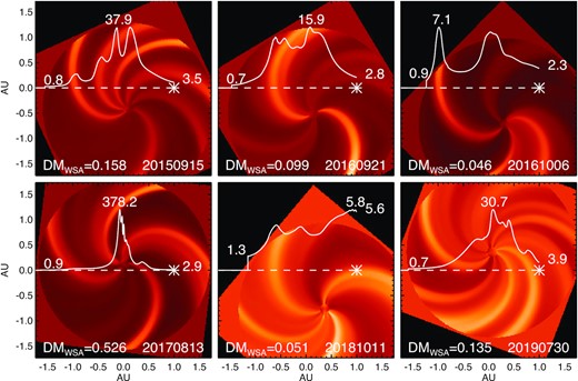
Illustrations of density profile measurement using wsa, for six epochs of B0950+08 at varying elongations. The circular part of each sub-image shows the density structure in the SW during a pulsar observation, divided by the azimuthally averaged radial density profile in order to emphasize structure and de-emphasize radial dependence. The centre of the circular region in each panel is the location of the Sun, the white asterisk towards the right marks the position of Earth, and the dotted line is the LoS to the pulsar (located to the left in each panel). The solid line is the density profile along the LoS, linearly scaled to the maximum density along the LoS (denoted above the peak). The SW density at Earth, and the density at the edge of the wsa region farthest from Earth along the LoS are also marked. The date is provided in the lower right of each panel, and the calculated wsa contribution to the DM is given in the bottom left.
4.3 Modelling the IISM contribution
In general both the SW and the IISM are contributing to the DMx contribution in any given measurement, and the two contributions need to be separated if we are to evaluate the effectiveness of SW models. We use the fact that the SW contributions to the DM are expected to be significant at small solar elongation angles, whereas at larger separations one expects DM variability to be dominated by the IISM. Our inferred SW contributions for different models were found to be about an order of magnitude smaller than the measured DMx values at angular separations >60° from the Sun.16 This suggests that even though there remains a scatter in the measured DMx values with solar elongation for some pulsars, those measurements are not dominated by the SW. Hence, as a starting point to model the contribution to DMs from the IISM, we choose a binning of our DMx values beyond 60° separation and apply a polynomial fit to estimate the expected IISM contribution at all separations. A linear fit was found to be sufficient to model these residuals, based on an F-test performed on the χ2 values of the fits for polynomials of order 1, 2, and 3. Applying the same procedure after binning the data at >30° separation in steps of 5° also gave similar values for the final residual rms. Other smaller separations were not tried because of possible contamination from the SW at smaller separations.
The resulting linear fits to the IISM contribution are shown as green lines in Fig. 2, where the DMx values are plotted as a function of date for all six pulsars. Fig. 3 shows the resulting dependence of DMx on solar elongation angle after the fitted IISM contributions have been subtracted: for all of the pulsars except B1257+12, the remaining DMx contributions show a pronounced dependence on solar elongation that starts to flatten out around zero beyond about 25−30° separation. Nevertheless, the data for B1257+12 show that this is not always the case. This may suggest that the IISM and SW behaviour are entangled at some level, and perhaps a more complex approach is required to separate cleanly the two contributions. A similar conclusion was also drawn by Tiburzi et al. (2019).
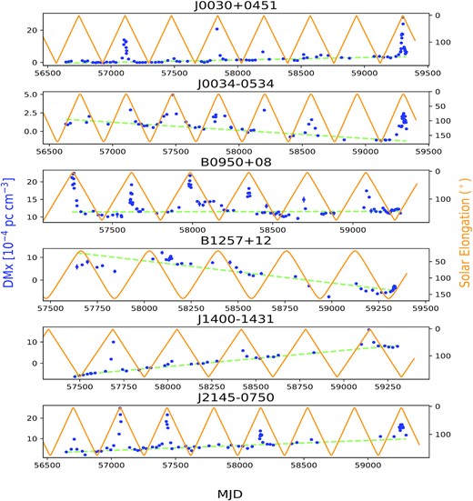
DM variation (DMx) time series for our pulsar sample. The blue points show the measured variations along with error bars measured using pulsar timing. The error bars are generally much smaller than the DMx values and so are not visible on the plot. The orange curve shows the angular separation between the pulsar and the Sun with the corresponding scale shown on the right axis. Each panel corresponds to a different pulsar. The dashed light green line shows the linear trend fitted as the IISM contribution.
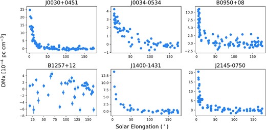
The plot of measured DMx with errorbars as a function of separation between the pulsar and the Sun. Each panel corresponds to a different pulsar. The fitted linear trend of the expected IISM contribution, as shown by the light green dashed line in Fig. 2, has been subtracted from the DMx values in each case to show the effect of SW contribution on DMx with solar elongation angle.
To minimize the possibility of entanglement in our IISM modelling, we also tried piecewise fitting of the data on annual time-scales, achieved by binning the data for separations larger than 60°, grouped between consecutive yearly near-Sun transits of the pulsar. No statistically significant improvements were seen based on an F-test performed on respective χ2 values from continuous and piecewise fitting for the case of a linear polynomial, except for PSR J1400−1431. However, even in that case the final residual rms for this pulsar did not improve as a result of the piecewise fitting. A similar analysis was not performed using higher order polynomials due to having insufficient points in a given bin to constrain the fitting parameters. Based on these results, we do not find any value in fitting more free parameters to the IISM variation than are needed for the linear polynomial fit in time using DMx values measured beyond 60° separation.
5 RESULTS
We analyse the DM variation with time for six pulsars over 7 yr, including five MSPs and a slow pulsar, and investigate the effectiveness of a range of SW models to account for the measured variations.
5.1 DM variation over time
Fig. 2 shows the variation of measured DM for the pulsar sample over time along with the corresponding solar elongation angle. The variations have been measured over 5−7 yr, depending on available data for different pulsars. Each of the pulsars shows evidence for a linear trend with time in DM at large elongations that can be attributed to variation in the IISM along the LoS to the pulsar. In particular, J1400−1431 shows a relatively sharp increase with time. The rate of change of the IISM contribution is not simply related to the total column to the pulsar, since J1400−1431 has a relatively low DM, similar to that of B0950+08 and J0030+0451, which do not show similar rates of change.
The behaviour of B1257+12 appears somewhat anomalous compared to the other five pulsars. While there is a general linear trend of decreasing DMx with time, it does not show the same striking dependence on solar elongation that the other pulsars share (Fig. 3 shows the dependence of pulsar DM after correction for IISM variation). Partly this is because its ecliptic latitude (17.6°) is significantly higher than the other sources, so its LoS never passes as close to the Sun, but there does seem to be little effect of solar distance in its data, and it exhibits a much larger scatter in measurements for elongations >30° than the other pulsars. PSR B1257+12 is a complex system: the pulsar is in orbit with a planetary system (e.g. Wolszczan 1994), and it may be that some of the orbital variations produce timing offsets that are not adequately fit by the orbital parameters in the timing model, and instead are absorbed in our analysis as spurious DM variations.
5.2 Comparison of SW models
Fig. 4 shows the DM residuals (DMx-SW-IISM, hereafter referred to as the residual) for the six pulsars with respect to different SW models, as a function of time. Regions of angular separations from the Sun below 20° are marked using black vertical lines. At larger angular separations, the residuals are close to zero. When the pulsar approaches the Sun, residuals are large, and no SW model provides a suitable correction. RMS values for the residuals were computed by binning them in the 15−40° elongation range in steps of 5°, as shown in Fig. 5. Table 2 reports the changes in RMS between 40° and 15° separation angle, with respect to the value at 40° separation. This was found to be |$30 {{\ \rm per\ cent}}$| or more for SW models other than wsa, with deviations in some cases as high as |$70 {{\ \rm per\ cent}}$|. For the case of the wsa SW model, the change was |${\sim} 15 {{\ \rm per\ cent}}$| or less for all pulsars. A similar comparison between 40° and 10° angular separation showed significantly higher RMS values, with up to twice larger values in some cases. Fig. 6 shows the residual RMS for each pulsar for each SW model. The lowest residual RMS are obtained in the case of the wsa model for each pulsar. A trend in residual RMS is seen, in that the RMS seems to increase with the pulsar spin period. A similar plot against ecliptic latitude did not show any trend in the calculated RMS values. Given the small number of pulsars in our sample it is difficult to claim if this trend is due to some causal relationship or related to some systematic in the data. For PSR B1257+12, the computed RMS were found to be significantly higher than the other pulsars, of the order of 10−4 pc cm−3.
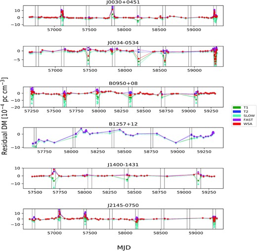
The final DM residuals after SW and IISM contributions are subtracted from the measured DMx. The different colours in the legend show the different SW models used to compute the residuals. The vertical black lines in the subplots mark the periods when the pulsar is at an angular separation of <20° from the Sun. For PSR B1257+12 there is no wsa plot since we did not calculate the wsa values in this case due to the higher ecliptic latitude of the pulsar. Residuals are plotted only for >4° separation because of large deviations below that.
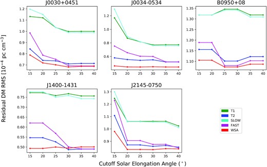
The calculated RMS of the DM residuals as a function of the cut-off solar elongation angle at 5° increments. The different colours show the different SW models used to calculate the residuals, as marked, and the panels correspond to different pulsars.
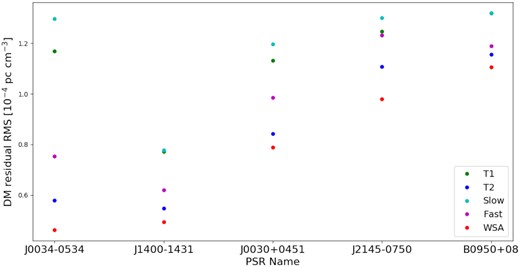
The RMS of the residual DM beyond 15° separation for each pulsar, with the results for the different SW models given by different colours in the plot legend. On the horizontal axis, the pulsar names are plotted in order of increasing spin period from left to right, based on the values given in Table 1.
This table shows the percentage change in calculated RMS values between cut-off angular separations of 40° and 15°, with respect to the value at 40°, for different pulsars and SW models.
| J0030+0451 | J0034−0534 | B0950+08 | J1400−1431 | J2145−0750 | |
|---|---|---|---|---|---|
| T1 | 13.2 | 51.2 | 0 | 2.2 | 21.7 |
| T2 | 18.1 | 11.7 | 3 | 11.7 | 30 |
| slow | 21.1 | 71.2 | 0.7 | 4.6 | 28.5 |
| fast | 42.5 | 44.4 | 7.8 | 26.5 | 45.5 |
| wsa | 14.6 | 3.6 | 1.7 | −1.5 | 16.8 |
| J0030+0451 | J0034−0534 | B0950+08 | J1400−1431 | J2145−0750 | |
|---|---|---|---|---|---|
| T1 | 13.2 | 51.2 | 0 | 2.2 | 21.7 |
| T2 | 18.1 | 11.7 | 3 | 11.7 | 30 |
| slow | 21.1 | 71.2 | 0.7 | 4.6 | 28.5 |
| fast | 42.5 | 44.4 | 7.8 | 26.5 | 45.5 |
| wsa | 14.6 | 3.6 | 1.7 | −1.5 | 16.8 |
5.3 DM derivatives
We quantify the overall DM trends by fitting a linear gradient to the data, using a least-square fitting routine, similar to Hobbs et al. (2004). However, since our sample data is solar-wind dominated at small solar elongations, we apply the gradient fitting after subtracting the calculated SW contribution to the DM, to avoid bias. As we work with five different models of SW, it results in five different values of these derivatives. Nevertheless, we see that these values, after different SW amplitude corrections, converge for data binned at >10° elongation angle. This is consistent with our previous results, where we see large amplitudes of DM residuals for small solar elongations. Hence, we report the amplitude of our DM derivatives as the mean of these five values (four in the case of B1257+12), where the error is calculated by adding the individual errors in quadrature. The corresponding values are reported in Table 3. To find the correlation between the DM and the amplitudes of its time derivatives, we fit a power law to this data. We get an exponent of 0.29 ± 0.65. Since this is consistent with the square root dependence in Hobbs et al. (2004), we also fit for the amplitude explicitly assuming a square root dependence, yielding ||$\frac{\rm d(DM)}{\mathrm{ d}t}$|| = 0.00005|$\sqrt{\mathrm{ DM}}$| for this small sample of pulsars, with negligible errorbars on the amplitude. This is a factor of 4 smaller than the Hobbs et al. (2004) estimate.
This table shows the average time derivative of DM after subtracting solar wind amplitudes and the median DM uncertainty of our data. The time derivative is calculated after binning the data SW model subtracted data for >10° elongation angle.
| J0030+0451 | J0034−0534 | B0950+08 | B1257+12 | J1400−1431 | J2145−0750 | |
|---|---|---|---|---|---|---|
| |$\frac{\mathrm{ d}\mathrm{ (DM)}}{\mathrm{ d}t} \left(\times 10^{-5} \frac{\mathrm{ pc}}{\mathrm{ cm}^{3}\, \mathrm{ yr}^{1}}\right)$| | 6.5 ± 1.2 | −5.0 ± 1.1 | 0.5 ± 1.9 | −31.5 ± 5.3 | 28.0 ± 1.2 | 10.5 ± 1.6 |
| |$M(\mathrm{ eDM})\ (\times 10^{-5} \,{\mathrm{ pc}}\,{\mathrm{ cm}^{-3}})$| | 3.0 | 0.65 | 2.67 | 5.98 | 0.94 | 2.53 |
6 DISCUSSIONS
For the sample of six pulsars examined in this study, each shows a significant DM variation over 5−7 yr. Measurement errors on DMx are an order of magnitude or lower than the corresponding DMx values for most observations, other than for PSR B1257+12, which is relatively weaker in our frequency bands. There is a clear dependence of the measured DM variations on the solar elongation angle for B0950+08, J0030+0451, J0034–0534, J1400–1431, and J2145–0750 marked by the sharp rise in values at separations less than ∼25−30°, as shown in Fig. 3.
For J1400–1431, we see the SW effect superimposed on a sharp upward trend of DMx, in time, as shown in Fig. 2. The robust linear increase in time for this pulsar is likely due to fluctuations in the local interstellar medium, as discussed below, and merits further investigation. It is worth pointing out that B0950+08, J0030+0451, and J1400−1431 are the lowest DM pulsars in the sample with comparable distance estimates as reported in the ATNF17 (Manchester et al. 2005) pulsar catalogue. Based on the proper motion values (in mas yr−1), J1400−1431 is the fastest moving pulsar, about twice faster than B0950+08, which is closer than the former. However, B0950+08 does not show a trend in DMx similar to that of J1400−1431, even if we were to consider data at separations of more than 40°, 50°, and 60° from the Sun. This suggests that the strong trend in DMx values for J1400−1431 cannot be explained as a simple increase in path-length through the IISM due to the pulsar’s proper motion, but rather suggests a role for spatial variations in the IISM.
B1257+12 does not show the same robust dependence of DMx on solar elongation angle seen in the other pulsars. Since its closest approach to the Sun is ∼17° and, as shown in Fig. 2, there is no clear correlation between its closest approach and corresponding peaks in the DMx values, it is possible that the DM variations are due to the combined effect of the SW and the complex orbit, which causes the scatter in DMx evident even at large separations.
Fig. 2 suggests some evidence for a change in the SW contribution over time due to the solar cycle: the height of the peaks in DMx at small elongations appear to change with time, although the sampling is insufficient for a strong conclusion. As an example, we measure DMx values of about 1.2, 2.0, and 1.7 (10−3 pc cm−3) for J0030+0451 at ∼5° elongation from the Sun, at different times, with similar errorbars, which are much smaller than the separation between these values. The same trend was seen even without any IISM component subtraction from the DMx data. In principle, the wsa model handles solar cycle variations since it is driven by measurements of the actual solar magnetic field, but the other models do not: this would require modelling of SW contributions with variable amplitude (see e.g. You et al. 2012; Tiburzi et al. 2019).
The calculated values of our DM time derivatives are comparable to those presented in Hobbs et al. (2004) and Jones et al. (2017) for PSR B1257+12 and J2145−0750, whereas for the other pulsars in common, the former has values that are two or more orders of magnitude larger than those presented here. A similar comparison shows that our values are in agreement with those reported in Donner et al. (2020), except for the case of B1257+12, which shows anomalous behaviour. One important difference between the two cases is the observing frequency. While the former two are primarily at high frequencies (>300 MHz), the latter is below 200 MHz, closer to the LWA frequencies that are more sensitive to DM variations. This reinforces the argument presented in Donner et al. (2020). Similarly, comparison of correlation between the amplitude of the DM time derivative and the DM magnitude shows that the time derivative follows a square root dependence consistent with Hobbs et al. (2004) and Donner et al. (2020). However, the amplitude of the square root dependence found here is comparable only with the latter study, being an order of magnitude smaller than the former.
6.1 Efficacy of SW models and IISM modelling
The residual DMs shown in Fig. 4 indicate that all SW models perform equally well at larger angular separations, but the situation changes at small elongations. The slow and fast wind models generally overestimate and underestimate the SW contributions, respectively, at smaller separations, creating larger DM residuals. Also, the spread in residuals (the measured RMS value) increases more steeply with decreasing separation for these models, as mentioned in Section 5.2, suggesting that the near-Sun application of these models is inadequate to capture fully the effects of the SW.
The spherical approximation models T1 and T2, where the former assumes the SW to be predominantly slow and the latter assumes it to be fast, perform slightly better than their respective slow and fast counterparts. The residuals, in this case, are smaller near the closest approach compared to the previous two. Moreover, the change in RMS with decreasing elongation for these two models is more gradual than the slow and fast cases.
The wsa operational model is found to give the best representation of the SW contribution to DMs, as the residuals are consistently the lowest and remain effective at smaller angular separations. The change in RMS with elongation is also more gradual, remaining below |$15 {{\ \rm per\ cent}}$| for all pulsars, whereas for other SW models, even though the change was |$\lt 25 {{\ \rm per\ cent}}$| for most pulsars, in some instances, it was up to |$50 {{\ \rm per\ cent}}$| or more. Hence, wsa keeps the residual RMS lower, irrespective of the pulsar. This is shown in Fig. 5, where the change in residual RMS with elongation for the wsa SW model is visibly smoother than for the other SW models.
As shown in Fig. 6, the measured RMS of the DM residuals are of the order of several 10−5 pc cm−3 for the MSP sample and slightly higher in the case of the slow pulsar B0950+08. The overall trend in the calculated RMS remains consistent across all pulsars, in decreasing order of slow, T1, fast, T2 and wsa SW models.
The appropriate modelling of the interstellar variations is also necessary in order to minimize DM residuals, especially at large separations where the SW effects are less significant. As discussed in Section 4.3, a few different approaches to this problem were investigated, but it was found that modelling the IISM behaviour as a linear polynomial in time is sufficient at the measurement level achieved in these data, at least over the 7-yr time-scale considered here. Even if this does not fully disentangle the SW and IISM effects, this should account for the slow variations due to the small change in the LoS to the pulsar, caused by the proper motion of a pulsar through the spatially varying interstellar medium.
6.2 Comparison with other low-frequency observations
For the common pulsars in our sample, we see similar trends in DM variations over long time-scales as reported in (see Donner et al. 2020; Krishnakumar et al. 2021; Tiburzi et al. 2021), where the former two are studies conducted below 200 MHz and the latter reports on observations above 400 MHz. While these are in agreement on the overall DM variation for these pulsars for the given span of time, the median uncertainties on our measured DM values, as reported in Table 3, are a factor 5–10 better than those in these studies, except for the case of B1257+12, where we get comparable values. Comparison of the expected RMS of time delay at 1400 MHz, as reported in Table 2, for the wsa model, with those shown in Tiburzi et al. (2021, fig. 5), shows that the wsa correction are better by a factor of 2 or more, depending on the pulsar, where Tiburzi et al. (2021) uses a constant and variable amplitude spherical SW model. This suggests that corrections provided by models informed by observations, like the wsa, provided improved corrections to SW effects.
6.3 Implications for PTAs
Inhomogeneity in the intervening medium can produce refractive effects and scattering of pulsar signals, resulting in different frequencies travelling slightly different paths through the medium. When the medium has significant fluctuations in free electron density on small spatial scales, the effective DM contribution seen by different frequencies can vary. Since the IISM is inhomogeneous, this is a direction-dependent effect. In order to assess the impact of our results on timing arrays that typically operate at frequencies higher than does LWA, we assume a frequency-independent value of DM (see e.g. Cordes, Shannon & Stinebring 2016; Lam et al. 2020) and use equation (1) to calculate the expected timing delay at 1.4 GHz, which is the commonly used frequency for PTA experiments. Fig. 7 shows the calculated delays for more than 15° separation, based on the DM residuals reported for the wsa model in Fig. 4. This is done by binning the DM residuals for >15° separation, for each pulsar after applying the wsa model and IISM contributions, and then calculating the expected delay for those values at 1.4 GHz using equation (1). The resulting RMS values of the timing residuals binned at 15° and 40° separations are reported in Table 4. We see that values are <300 ns in all cases, and in some cases are as small as 100 ns even at 15°, as desired for PTA experiments. The expected RMS of timing residuals will be higher in the case of the other SW models discussed here. Nevertheless, the RMS of DM residuals achieved for our sample is of the order of 10−5 pc cm−3 for PTA-class pulsars, which is significantly better than the reported median DM uncertainty of the order of 5 × 10⁻⁴ pc cm−3 for PTA experiments (see e.g. Alam et al. 2021). Hence, low-frequency observation of those pulsars could improve the noise limits in timing experiments by reducing the timing noise due to DM uncertainties. There are two possible scenarios, the first being a simultaneous observation of the pulsar at low frequencies and using the measured DM to correct the TOAs in the high-frequency data. The second is regular monitoring of the pulsar at low frequencies to model the slow trends due to the IISM, combined with high-cadence observations (possibly same day) during the closest approach of the pulsar LoS to the Sun to obtain corrections due to the SW. As the SW is highly variable, low-frequency observations close to the high-frequency PTA observations are necessary to avoid introducing excess noise in the data. Some improvement could also be obtained by applying the wsa model rather than the default model used in PTA data analysis. Also, as we move into an observing cycle of increasing solar activity, using a model that is not stationary in time would be more appropriate to mitigate the SW effects, since it can capture the variable nature of the SW. There are two different approaches that could be employed to this effect: (1) using an existing SW model like the wsa, which is driven by parameters from independent cotemporaneous observations of the Sun, or (2) to perform very high cadence observations of a pulsar at low radio frequency and using these observations to perform an amplitude scaling of the stationary models of the SW such as T1, T2, etc., which has already been suggested in some previous studies. However, any such amplitude modelling would need to be tested against other measurements of SW, so as to avoid any biases that may be introduced due to pulsars in the sample data.

The calculated time delays at 1.4 GHz for angular separations of more than 15° solar elongation angle. The values are based on the corresponding DM residuals for the wsa SW model.
Table of expected RMS of time delay at 1.4 GHz based on the residual DMs calculated at our frequencies. RMS40 is for angular separation of more than 40° and RMS15 is similarly for 15° separation.
| J0030+0451 | J0034−0534 | B0950+08 | J1400−1431 | J2145−0750 | |
|---|---|---|---|---|---|
| RMS15 (µs) | 0.167 | 0.098 | 0.234 | 0.104 | 0.207 |
| RMS40 (µs) | 0.146 | 0.094 | 0.230 | 0.106 | 0.178 |
| J0030+0451 | J0034−0534 | B0950+08 | J1400−1431 | J2145−0750 | |
|---|---|---|---|---|---|
| RMS15 (µs) | 0.167 | 0.098 | 0.234 | 0.104 | 0.207 |
| RMS40 (µs) | 0.146 | 0.094 | 0.230 | 0.106 | 0.178 |
7 SUMMARY AND CONCLUSIONS
We have studied SW effects and IISM variation in a sample of six pulsars using 5−7 yr of available data. Five different SW models have been investigated, providing different levels of precision for DM measurements. The commonly used spherical SW models perform better than assumptions of slow or fast approximations of the SW. The measured DM residuals are comparatively smaller, in this case, up to solar elongation angle of ∼25−30°. However, there is a swift change in RMS values at closer separations due to insufficient correction for the SW. As the simplest spherical models have a time-constant amplitude of SW correction, they also fail to account for the change in SW activity during a solar cycle on longer time-scales, but a time-dependent version of the model can be applied, as shown by Tiburzi et al. (2019). Nevertheless, this study shows that the spherical model does not work equally well for all pulsars, as some pulsars show a more significant change in residual RMS as the pulsar approaches close to the Sun.
wsa is the other SW model investigated in this paper, applied to operational space weather forecasting by using observations of solar magnetic fields to drive a time-dependent model of the SW, as well as to catch CME transients directed towards the Earth. Implementation of the wsa model for measuring the SW effect in low-frequency timing data provides the smallest DM residuals. At the same time, it is equally effective for all pulsars in our sample, with a change in residual RMS below |$15 {{\ \rm per\ cent}}$| in all cases between 40° and 15° angular separations. Hence, this model remains effective even at a closer approach to the Sun. In order to constrain the RMS of DM residuals given by these cut-off angular separations, we need to avoid observation windows of 30 and 80 d for 15° and 40° cut-off angular separations between the pulsar LoS and the Sun. This would amount to losing |${\sim}9$| and |$22 {{\ \rm per\ cent}}$| of the total observing time, respectively.
These SW models can be used to some extent down to 10° separation, but with significantly higher residuals. None of the models work well below 10°. However, since high-precision pulsar timing experiments generally tend to avoid an observation window (∼10−15 d) near the solar conjunction of the pulsar, it is safe to assume that corrections at those separations would not be required.
In this study, we used archival wsa data from the daily operational runs provided by NOAA in order to test the value of more sophisticated SW models for correcting pulsar DMs. This data source has the advantage that the complex 3D MHD models have already been run for essentially every day for which we have pulsar data, but the disadvantage that (in order to reduce file sizes) only 2D data in the ecliptic plane can be used and this is obviously not satisfactory for wider application. However, suitable 3D models are available: NASA’s Community Coordinated Modelling Center provides runs-on-demand for a number of models, including wsa.18 Other approaches may also prove fruitful, such as the SW model derived from observations of interplanetary scintillation (Jackson et al. 2011). We are in the process of exploring approaches to provide high-quality 3D SW models suitable for routine estimation of DM contributions for pulsar timing applications.
Even though we find that these SW models do not consistently reach the 100 ns timing accuracy desired by PTA experiments, using these SW models and low-frequency pulsar observation, we were able to achieve an RMS on DM residuals of the order of several 10−5 pc cm−3, which is better than existing values for PTAs. Hence, using low-frequency observations could be helpful to improve the noise limits in PTA experiments by minimizing the effect of DM variations and allowing for the inclusion of observations at smaller solar elongation angles. Low-frequency pulsar observations can also be used to test the efficacy of other space weather models. We also found that the variations in IISM contribution were slower than suggested by Hobbs et al. (2004), which suggests that low-frequency observations at large angular separations from the Sun are equally important, for PTAs as well as to study the spatial and temporal structure of IISM variations.
Similar studies with a larger sample of pulsars with existing and upcoming low-frequency facilities could help to improve SW and IISM models. Combining the data from multiple low-frequency observations, which are most sensitive to DM variations, can improve observing cadences and increase bandwidths, allowing for the study of these variations on shorter time-scales. This could potentially provide a detection of the variation in DM, SW activity, or IISM behaviour with frequency.
ACKNOWLEDGEMENTS
We thank the referee for constructive suggestions. Construction of the LWA has been supported by the Office of Naval Research under contract N00014-07-C-0147 and by the AFOSR. Support for operations and continuing development of the LWA1 was provided by the Air Force Research Laboratory and the National Science Foundation under grants AST-1835400 and AGS1708855. We thank NOAA’s National Centers for Environmental Information (NCEI) for archiving the wsa-enlil data used in this study (https://dx.doi.org/10.7289/V5445JGH).
DATA AVAILABILITY
All the pulsar data used in this paper are publicly available on the LWA Pulsar Archive as mentioned in Section 2. The wsa archive files are publicly available at https://www.ngdc.noaa.gov/enlil/.
Footnotes
LWA Pulsar Archive: https://lda10g.alliance.unm.edu/PulsarArchive/.
Global Oscillations Network, https://gong.nso.edu/.
Synoptic Optical Long-term Investigations of the Sun, https://nso.edu/telescopes/nisp/solis/.
Helioseismic and Magnetic Imager on NASA’s Solar Dynamics Observatory, http://hmi.stanford.edu/.
Air Force Data Assimilative Photospheric Flux Transport model.
Note that we do not calculate contributions from the wsa model for separations beyond 60°, since the outer radius of 1.7 au in the model means that not much of the wind is being sampled.
