Measuring the Milky Way mass distribution in the presence of the LMC Free

Parameters of the fiducial mock data set. First two columns define the tracer populations (globular clusters and satellite galaxies), which are the same in other mock data sets; third column defines the MW (spherical halo-only model), last column defines the LMC. The density of all components follows a tapered double power-law profile (equation 4), and the DF is given by the Cuddeford (1991) inversion formula with the central anisotropy coefficient β₀ and anisotropy radius r_a.

	GC	Sat	MW halo	LMC
Total mass (⁠\|$10^{12}\, \mathrm{M}_\odot$\|⁠)	Negligible		1.1	0.15
Scale radius r_scale (kpc)	5	100	5	10.8
Cut-off radius r_cut (kpc)	∞		290	108
Cut-off strength ξ	n/a		2	2
Inner slope γ	0.0	0.5	1.0	1.0
Outer slope β	6.0	6.0	3.0	3.0
Transition steepness α	0.5	2.0	0.5	1.0
Central anisotropy β₀	0.0	−0.4	0.0	0.0
Anisotropy radius r_a (kpc)	25	200	∞

	GC	Sat	MW halo	LMC
Total mass (⁠\|$10^{12}\, \mathrm{M}_\odot$\|⁠)	Negligible		1.1	0.15
Scale radius r_scale (kpc)	5	100	5	10.8
Cut-off radius r_cut (kpc)	∞		290	108
Cut-off strength ξ	n/a		2	2
Inner slope γ	0.0	0.5	1.0	1.0
Outer slope β	6.0	6.0	3.0	3.0
Transition steepness α	0.5	2.0	0.5	1.0
Central anisotropy β₀	0.0	−0.4	0.0	0.0
Anisotropy radius r_a (kpc)	25	200	∞

Table 1.

Parameters of the fiducial mock data set. First two columns define the tracer populations (globular clusters and satellite galaxies), which are the same in other mock data sets; third column defines the MW (spherical halo-only model), last column defines the LMC. The density of all components follows a tapered double power-law profile (equation 4), and the DF is given by the Cuddeford (1991) inversion formula with the central anisotropy coefficient β₀ and anisotropy radius r_a.

	GC	Sat	MW halo	LMC
Total mass (⁠\|$10^{12}\, \mathrm{M}_\odot$\|⁠)	Negligible		1.1	0.15
Scale radius r_scale (kpc)	5	100	5	10.8
Cut-off radius r_cut (kpc)	∞		290	108
Cut-off strength ξ	n/a		2	2
Inner slope γ	0.0	0.5	1.0	1.0
Outer slope β	6.0	6.0	3.0	3.0
Transition steepness α	0.5	2.0	0.5	1.0
Central anisotropy β₀	0.0	−0.4	0.0	0.0
Anisotropy radius r_a (kpc)	25	200	∞

	GC	Sat	MW halo	LMC
Total mass (⁠\|$10^{12}\, \mathrm{M}_\odot$\|⁠)	Negligible		1.1	0.15
Scale radius r_scale (kpc)	5	100	5	10.8
Cut-off radius r_cut (kpc)	∞		290	108
Cut-off strength ξ	n/a		2	2
Inner slope γ	0.0	0.5	1.0	1.0
Outer slope β	6.0	6.0	3.0	3.0
Transition steepness α	0.5	2.0	0.5	1.0
Central anisotropy β₀	0.0	−0.4	0.0	0.0
Anisotropy radius r_a (kpc)	25	200	∞

We then run a conventional N-body simulation of the encounter between the MW and the LMC, using the code gyrfalcON (Dehnen 2000). We choose the initial position and velocity of the LMC in such a way that it arrives at the observed point³ after 2 Gyr of evolution. The initial guess for the starting point is given by integrating the equations of motion of two galaxies (equation 1), and then we iteratively refine it by running a suite of six simulations with slightly different initial conditions, computing the Jacobian of transformation between the start and end points, and using the Gauss–Newton method to update the initial point, as described in section 3.2 of Vasiliev et al. (2021a). The final LMC position and velocity matches the actual observations to ∼0.1 kpc and ∼0.5 km s⁻¹. We extract the trajectories of the MW and LMC centres from the N-body simulation (using centre-of-mass position and velocity iteratively determined from particles within the central 10 kpc for each galaxy), fit a smooth spline curve to the former and differentiate it twice to obtain the acceleration of the MW-centred non-inertial reference frame. The positions and velocities of tracer particles at the final snapshot are used to construct the ‘present-day’ mock data set, and we also use their initial coordinates to test the method on the unperturbed MW system.

3.2 LMC orbit reconstruction

The first question to be explored quantitatively is the accuracy of the LMC orbit reconstruction with our orbit-rewinding procedure (equation 1). Fig. 1 shows the time evolution of three components of the relative separation between LMC and MW centres (top row) and three components of the Galactocentric reference frame acceleration (bottom row), for two simulations with the same MW model but LMC masses of 10¹¹ and |$2\times 10^{11}\, \mathrm{M}_\odot$|⁠. The only adjustable parameter in this rewinding procedure is the Coulomb logarithm ln Λ. By examining these and a few other simulations, we settle on the following expression, which provides an adequate match to N-body orbits in all cases: ln Λ = ln [D_LMC(t)/ϵ_LMC]. Here, D_LMC(t) is the instantaneous distance between the LMC and the MW centre, and ϵ_LMC is the effective ‘softening radius’, for which the value 2 × r_scale appears to be optimal (it varies between 17 and 26 kpc for the two limiting values of LMC mass we considered). This functional form was also used by Jethwa et al. (2016) in the same context, although they found that their N-body trajectories were better matched by a somewhat lower ϵ_LMC in the Coulomb logarithm.

$Reconstruction of LMC’s past orbit with the approximate solution of two extended bodies’ equations of motion. Top row shows the three Cartesian components of relative distance between the MW and LMC centres, bottom row shows the components of MW’s acceleration. Solid lines are taken from a live N-body simulation, dashed lines are the orbits reconstructed via equation (1). Thinner and thicker lines show two cases: $M_\text{LMC}=10^{11}\, \mathrm{M}_\odot$ and $2\times 10^{11}\, \mathrm{M}_\odot$, respectively; the MW potential is the same in both cases. Overall, the approximate solution reproduces the actual orbits reasonably well over the relevant range of LMC masses, at least over the last Gyr when the effect of the LMC flyby is most significant, although the MW acceleration is slightly overestimated by the approximation.$

Figure 1.

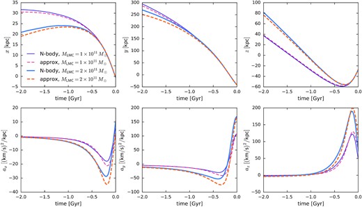
Reconstruction of LMC’s past orbit with the approximate solution of two extended bodies’ equations of motion. Top row shows the three Cartesian components of relative distance between the MW and LMC centres, bottom row shows the components of MW’s acceleration. Solid lines are taken from a live N-body simulation, dashed lines are the orbits reconstructed via equation (1). Thinner and thicker lines show two cases: |$M_\text{LMC}=10^{11}\, \mathrm{M}_\odot$| and |$2\times 10^{11}\, \mathrm{M}_\odot$|⁠, respectively; the MW potential is the same in both cases. Overall, the approximate solution reproduces the actual orbits reasonably well over the relevant range of LMC masses, at least over the last Gyr when the effect of the LMC flyby is most significant, although the MW acceleration is slightly overestimated by the approximation.

As seen from the above figure, the LMC rewinding prescription adequately recovers the time evolution of the MW–LMC separation in N-body simulations, but overestimates the MW acceleration around the its peak by ∼20 per cent (40 per cent) for the x (y) components. This could be attributed to the neglect of the developing deformation of the MW: we implicitly assume that the entire Galaxy is pulled towards the LMC with spatially uniform acceleration, but in reality the swinging motion of the inner MW towards the LMC is partly counteracted by the gravitational force from the outer MW halo, which reacts more slowly (see Vasiliev et al. 2021b for an in-depth discussion). Although not perfectly reconstructed, the x- and y-components of MW acceleration change sign during the interaction, and the accumulated changes in the MW reflex velocity are smaller than in the z-component (∼20 km s⁻¹ versus ∼50 km s⁻¹, see fig. 10 in Vasiliev et al. 2021a); the latter is the dominant cause of the kinematic asymmetry illustrated later in Fig. 7, and is recovered to within a few km s⁻¹.

It is also interesting to note that the effect of changing the LMC mass is sublinear, and that the more massive LMC actually needs to start at a smaller distance in order to arrive to the same present-day point. This contrasts a simple picture used in earlier studies, in which the back-reaction of the LMC on the MW would be neglected, and LMC would move in a fixed external potential subject to additional dynamical friction force: in this case, more massive LMC would lose more energy and would have to start at a less bound orbit (i.e. further out and with a higher inward velocity), as seen, for instance, in fig. 9 of Kallivayalil et al. (2013). Our orbit-rewinding scheme follows the mutual forces and motion of both galaxies, and is thus able to reproduce this nonlinear effect, but will likely break down for even higher LMC masses. For this reason, we put an upper limit of |$2.5\times 10^{11}\, \mathrm{M}_\odot$| for M_LMC in the fit, but fortunately, the best-fitting models do not hit this boundary.

3.3 Orbit rewinding in the time-dependent potential

After confirming that the LMC trajectory can be reconstructed reasonably well, we now turn to the second part of the orbit rewinding scheme – integrating the tracer orbits back in time from their present-day coordinates in an evolving potential composed of a moving LMC, fixed analytic potential of the MW, and time-dependent but spatially uniform acceleration of the Galactocentric reference frame. Fig. 2 shows a few typical orbits: the original particle trajectories in the N-body simulation are reasonably well-approximated by the time-dependent orbit rewinding, but much less well by orbits in a static MW potential alone. Although some phase differences between the original and the reconstructed orbit inevitably accumulate over time, these are unimportant for the purpose of DF fitting, which uses only the integrals of motion but not phases. The relative error in position grows approximately linearly with lookback time and is at the level ∼0.1 (median) for the time-dependent orbit reconstruction, while being ∼5 times higher for the static potential.

Figure 2.

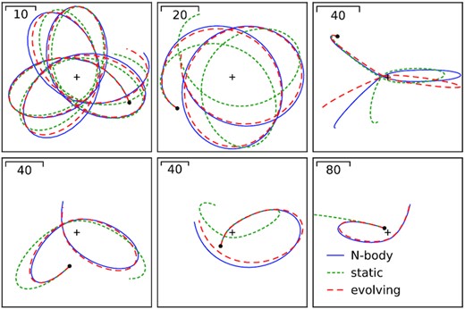
Illustration of the accuracy of orbit rewinding for several representative orbits. Black cross is the MW centre; black dots mark the present-day positions; blue solid lines show the trajectories of particles in the original N-body simulation; red-dashed lines are orbits integrated back in time from the present-day snapshot in the evolving MW + LMC potential; and green short-dashed lines are the orbits integrated in a static MW potential. The latter are often very different from the true ones, at least in the outer parts of the Galaxy, while the rewinding in a time-dependent potential reproduces the original trajectories ∼5 × better.

Fig. 3 presents a different view on the LMC perturbation, showing the energy changes of particles in the actual N-body simulation at different radii (blue contours). These changes are relatively small and likely caused by numerical relaxation effects in the inner part of the system, but are much more prominent beyond 20–30 kpc (here, the horizontal axis is not the instantaneous radius of a particle, but the radius of a circular orbit with the same energy, i.e. close to a time-averaged orbit size). The energy of individual particles may increase or decrease, but on average it increases more often (note the asymmetry of the 1D histogram of ΔE in the right-hand panel). The orbit rewinding in a time-dependent potential recovers the initial particle energies fairly well, as shown by a much tighter and symmetric distribution of the difference between reconstructed and actual initial energies (the r.m.s. error in energy is |$\sim 10^3\, \big [\text{km s}^{-1}\big ]^2$| for the time-dependent reconstruction and ∼5 times higher in the static potential). Since the most bound orbits are little affected by the LMC, we may save effort by performing rewinding only for orbits with energies corresponding to the radii of circular orbits ≥10 kpc, safely including the entire region of significant perturbations shown by blue contours in that figure.

Figure 3.

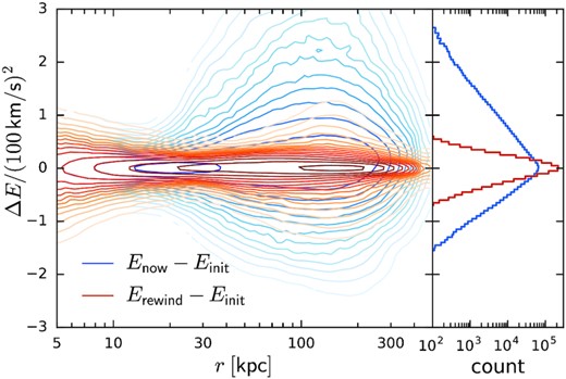
Illustration of the accuracy of orbit rewinding. Shown are density plots of particle energy changes as a function of radius; contours are logarithmically spaced by factors of two in density. Blue contours show the changes in particle energies due to the LMC perturbation in the N-body simulation. Red contours show the difference between the energy of the reconstructed initial snapshot (rewinding orbits from the present-day state backward in time in the evolving analytic MW + LMC potential) and the actual initial energy of the same particles in the simulation. In the ideal case, this difference would be zero; in practice, it has some residual scatter, but much narrower than the actual energy changes. The imperfect reconstruction is likely caused by inaccuracy of the original N-body simulation (numerical heating in the inner few kpc, where the LMC plays no role) and the neglect of MW deformation in the orbit rewinding scheme at larger radii.

Having demonstrated the accuracy of the orbit rewinding scheme, we now scrutinize the performance of the DF fitting approach itself.

3.4 Measurement of the MW potential

We ran the fitting routine for several choices of the MW potential and LMC mass, which all displayed similar performance. In this section, we discuss the fiducial case of a |$1.5\times 10^{11}\, \mathrm{M}_\odot$| LMC in a spherical MW potential with the total mass |$1.1\times 10^{12}\, \mathrm{M}_\odot$|⁠, using either the globular cluster sample, the satellite sample, or both. For each mock data set, we consider three scenarios: (1) initial, unperturbed MW potential; (2) present-day MW affected by the LMC, but ignoring it during the fit; (3) present-day MW with orbit rewinding compensating the LMC perturbation.

Fig. 4, top row, shows the results of these experiments on the full sample of tracers (1000 objects in each data set). These ideal conditions illustrate that each of the two data sets produces tight constraints around the median radius of tracer points (∼5 kpc for globular clusters and ∼100 kpc for satellites), and uncertainties increase considerably outside the range spanned by tracers, which is natural to expect if the model for the potential is flexible enough. In the unperturbed case, the mass distribution is recovered very well, and applying the vanilla DF-fitting method to a perturbed snapshot overestimates the mass at radii r ≳ 30 kpc by ∼20–30 per cent, in agreement with Erkal et al. (2020). Most interestingly, the addition of the orbit-rewinding step brings the inferred mass profile quite close to truth, which is very encouraging. We note that the inference is still slightly biased at r ≲ 10 kpc, but at these radii the MW potential is better measured with alternative methods.

$Tests of the method on mock data sets, described in Section 3.1: top row shows large data sets (1000 objects in each), bottom row – realistic sizes (150 globular clusters and 50 satellites). Each panel shows the inferred circular-velocity profiles $v_\text{circ}(r) \equiv \sqrt{G\, M(\lt r)/r}$ for two mock catalogues, representing globular clusters (red) and satellites (blue), and in the bottom row, the combined sample (green); the true profile is plotted by a black dashed curve. Solid lines show the medians, while darker and lighter shaded regions indicate 16/84 and 2.3/97.7 percentiles (‘1σ’ and ‘2σ’ confidence intervals). Naturally, the constraints are tightest in different radial ranges for the two data sets: around 5–10 kpc for clusters and 100 kpc for dSph. Left-hand panel shows the initial, unperturbed system before the arrival of the LMC, which illustrates excellent performance of the method in the ideal case. Centre panel shows the fit for the present-day snapshot perturbed by the LMC, but without accounting for it in the model, which leads to an overestimate of enclosed mass beyond a few tens kpc. Right-hand panel demonstrates that with the orbit rewinding scheme in place, the model is able to recover the true potential.$

Figure 4.

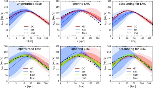
Tests of the method on mock data sets, described in Section 3.1: top row shows large data sets (1000 objects in each), bottom row – realistic sizes (150 globular clusters and 50 satellites). Each panel shows the inferred circular-velocity profiles |$v_\text{circ}(r) \equiv \sqrt{G\, M(\lt r)/r}$| for two mock catalogues, representing globular clusters (red) and satellites (blue), and in the bottom row, the combined sample (green); the true profile is plotted by a black dashed curve. Solid lines show the medians, while darker and lighter shaded regions indicate 16/84 and 2.3/97.7 percentiles (‘1σ’ and ‘2σ’ confidence intervals). Naturally, the constraints are tightest in different radial ranges for the two data sets: around 5–10 kpc for clusters and 100 kpc for dSph. Left-hand panel shows the initial, unperturbed system before the arrival of the LMC, which illustrates excellent performance of the method in the ideal case. Centre panel shows the fit for the present-day snapshot perturbed by the LMC, but without accounting for it in the model, which leads to an overestimate of enclosed mass beyond a few tens kpc. Right-hand panel demonstrates that with the orbit rewinding scheme in place, the model is able to recover the true potential.

As expected, the uncertainties grow considerably when we reduce the tracer sample to a more realistic size: 150 clusters and 50 satellites. The inferred mass profile becomes rather sensitive to the choice of the random sample (i.e. to the Poisson noise), although still remains statistically consistent between different samples due to large uncertainty intervals. The bottom row of Fig. 4 shows one of the least biased samples, illustrating the same trends as for the large sample test; in other cases, the median inferred profiles may shift up or down by a few tens per cent, but the relative effect of adding the LMC perturbation and accounting for it during the fit remains the same. When we perform the fit simultaneously for both data sets, the uncertainties ‘take the best of both worlds’ and become rather small in the entire radial range, also stabilizing the results against random fluctuations caused by a small sample size.

Finally, we consider the effect of adding measurement errors: 0.1 for the distance modulus (4.7 per cent relative distance error), 0.05 mas yr⁻¹ for PM, and 2 km s⁻¹ for the line-of-sight velocity. These are relatively small errors, but if we ignore them in the fit, the inferred mass is biased up by 12 per cent at 100 kpc and by 30 per cent at 200 kpc. On the other hand, taking them into account restores the unbiased inference at large radii, while increasing the uncertainty intervals only slightly (by 10–20 per cent): in other words, the finite sample size (Poisson noise) is far more important than measurement errors. The green curves in the bottom panel show the fits to the combined data set with measurement errors, which still have fairly small uncertainty intervals and recover the enclosed mass profile to within |$\sim 10{{\ \rm per\ cent}}$| at all radii.

The average log-likelihood of models without orbit rewinding (i.e. with biased potential inference) is lower than models with rewinding by |$\Delta \ln \mathcal {L}\sim 5\!-\!10$| for the cluster sample and 10–15 for the satellite sample, i.e. the non-zero LMC mass is preferred at high significance. In fact, the relative uncertainty on M_LMC is at the level of 30 per cent when using only satellites, and twice larger when using only clusters; in the combined fit, satellites dominate. The best-fitting LMC mass agrees with the true value within uncertainties.

The above results were obtained for a spherical MW model and using a QuasiSpherical DF of tracers. We also ran the analysis pipeline on the same mock data set, but using DoublePowerLaw action-based DF (equation 5) in the fit (thus different from the actual DF used to construct the sample), obtaining very similar constraints for the potential and recovering the kinematic profiles of the tracer populations. Finally, additional experiments were run with non-spherical MW models taken from Vasiliev et al. (2021a) and DoublePowerLaw tracer DFs, again recovering the potential with good accuracy (typically within 10 per cent at all radii).

4 APPLICATION TO THE MILKY WAY

4.1 Input data

We use two classes of dynamical tracers – globular clusters and satellite galaxies. The former are more likely to be orbiting in the MW for many Gyr and thus are expected to be well mixed and satisfy the assumptions of equilibrium dynamical models (in absence of the LMC), but are mostly concentrated in the inner 10–20 kpc of the Galaxy, where the LMC does not cause a significant perturbation. Satellite galaxies, on the other hand, are located much further out, at a typical distance of ∼100 kpc, but present an additional complication as some of them might have been accreted into the MW system only recently and thus not yet fully virialized. This certainly applies to objects at distances comparable to or exceeding the virial radius (250–300 kpc), such as Eridanus II, Leo T, or Phoenix, which are still on the way towards the MW, but also possibly to galaxies that have already passed their pericentre, but still have high energy, such as Leo I. The latter object is especially troublesome, with its distance of ∼250 kpc and heliocentric reflex-corrected (‘Galactic standard of rest’) line-of-sight velocity of 167 km s⁻¹ making it difficult to reconcile with being a long-term bound satellite, unless the MW mass exceeds |$\sim 1.5\times 10^{12}\, \mathrm{M}_\odot$| (e.g. Kulessa & Lynden-Bell 1992; Boylan-Kolchin et al. 2013).

For the globular cluster population, we use the most recent distance, PM, and line-of-sight velocity measurements from Baumgardt & Vasiliev (2021), Vasiliev & Baumgardt (2021), and Baumgardt et al. (2019), respectively. The entire catalogue contains 170 objects, but nine of them (all at distances below 50 kpc) lack line-of-sight velocity measurements. Although data points with missing dimensions can still be used in model fitting, they add very little to model constraints, so we exclude them for simplicity. Furthermore, we exclude the seven clusters associated with the Sagittarius dSph and its stream: NGC 6715 (M 54), Arp 2, Terzan 7, Terzan 8, Pal 12, Whiting 1, and NGC 2419.

For the satellite population, we primarily use the most complete compilation of PM measurements and other properties by Battaglia et al. (2022, tables B1 and B2), but also rerun some of our fits with alternative PM catalogues of McConnachie & Venn (2020) and Li et al. (2021), which are also based on Gaia EDR3: the results were robust w.r.t. the choice of the PM data set. These catalogues are not limited to the MW satellites, but contain other galaxies from the Local Group; we limit the sample to galaxies within 300 kpc, and likewise exclude objects without line-of-sight velocity measurements (although we examine their possible orbits in the potential models determined in our fit). We also remove the Small Magellanic Cloud (SMC) and other galaxies possibly associated with the LMC, as discussed by Battaglia et al. (2022): Carina II, Carina III, Horologium I, Horologium II, Hydrus I, Phoenix II, and Reticulum II; again, we revisit their orbits after running the fits. Finally, we exclude a few objects that have unreliable PM measurements or are possibly unbound: Columba I, Pegasus III, Pisces II, and Reticulum III. This leaves us with a sample of 36 galaxies: Antlia II, Aquarius II, Boötes I, Boötes II, Boötes III, Canes Venatici I, Canes Venatici II, Carina, Coma Berenices, Crater II, Draco, Draco II, Fornax, Grus I, Grus II, Hercules, Hydra II, Leo I, Leo II, Leo IV, Leo V, Sagittarius, Sagittarius II, Sculptor, Segue 1, Segue 2, Sextans, Triangulum II, Tucana II, Tucana III, Tucana IV, Tucana V, Ursa Major I, Ursa Major II, Ursa Minor, and Willman 1.

We propagate the measurement errors into Galactocentric positions and velocities, drawing 100 (for globular clusters) or 1000 (for satellites) Gaussian random samples from the quoted uncertainties, imposing a lower limit of 0.02 mas yr⁻¹ for the PM error, and 0.05 mag (for clusters) or 0.1 mag (for satellites) on the distance modulus. The results are fairly insensitive to the number of samples, since the observational uncertainties are typically quite small, with a few exceptions discussed later. However, for objects lacking line-of-sight velocities, we would have to use a larger number of samples covering a wide range of possible values, or design a more sophisticated importance sampling scheme, as in Read et al. (2021), which is the main reason for excluding them. We also add uncertainties on the Solar position and velocity: x_⊙ = −8.12 ± 0.1 kpc, |$v_\odot =\lbrace 12.9\pm 1,\, 245.6\pm 3,\, 7.8\pm 1\rbrace$| km s⁻¹ (Drimmel & Poggio 2018).

4.2 Model specifications

We first consider the two data sets independently, running separate fits for globular clusters and satellites. In each case, we use the DoublePowerLaw DF family for the tracers (equation 5), which has nine free parameters; simpler QuasiSpherical DF models are less flexible and produce noticeably worse fits (with a difference in log-likelihood |$\Delta \ln \mathcal {L} \gtrsim 5$| for dSph alone), justifying the extra three parameters responsible for a non-spherical tracer density distribution and rotation. The MW halo is represented by a spherical Zhao (1996) model (Spheroid density profile, equation 4) with five free parameters: inner and outer slopes γ, β, transition steepness α, scale radius r₀, and corresponding density ρ₀. The outer slope β is allowed to be shallower than three (the value for the NFW profile), which formally corresponds to an infinite mass (we do not impose exponential truncation in these models); as long as β > 2, the potential still tends to zero at infinity, and the entire procedure remains valid. In contrast to many other studies (e.g. Eadie & Juric 2019; Deason et al. 2021), we do not artificially narrow down the prior range on any of the model parameters based on some cosmological simulations, but consider widest possible range of models and let the data speak for itself. However, to explore the sensitivity of results to the chosen parametrization of the halo density, we additionally ran another series of models with the exponential Einasto (1965) profile, which has three free parameters: cut-off radius r_cut, steepness ξ, and normalization ρ₀. We experimented with non-spherical, constant-axis-ratio models, but found that the axial ratio q = z/x, although not well constrained, prefers values closer to unity. Since the Stäckel fudge is designed only for oblate or spherical potentials, we could not check if prolate models would provide a better fit.⁴

We fix the parameters of the baryonic components to the values taken from the McMillan (2017) best-fitting potential. The bulge is a flattened truncated power-law model with γ = β = 1.8, α = 1, r_cut = 2.1 kpc, axial ratio q = 0.5, and total mass |$M=0.9\times 10^{10}\, \mathrm{M}_\odot$|⁠. We use a single exponential disc component in place of two stellar and two gas discs to simplify and speed up computations; it has a total mass |$5.6\times 10^{10}\, \mathrm{M}_\odot$|⁠, scale radius 3 kpc, and scale height 0.3 kpc. In principle, one could allow these parameters to vary, but doing so introduces degeneracy in the total potential, which should be balanced by additional observational constraints, e.g. the dependence of vertical force on z inferred from stellar kinematics in the Solar neighbourhood. Since our primary goal is to explore the potential at large scales, and because the axisymmetric assumption of the Stäckel fudge is violated in the inner Galaxy anyway, we ignore these complications, and instead pin the circular-velocity curve at the Solar radius to 235 ± 10 km s⁻¹ (McMillan 2017), adding a corresponding term to the likelihood function (although the results change very little if we remove this constraint). This model setup is nearly identical to the one used in Vasiliev (2019b). We also explored the effect of adding measurements of the circular velocity from Eilers et al. (2019): these provide very tight constraints on the circular velocity profile at radii 5 ≤ R ≤ 25 kpc, but otherwise little affect the inferred mass distribution at large radii.

The LMC mass is another free parameter with a log-flat prior and an upper limit of |$3\times 10^{11}\, \mathrm{M}_\odot$|⁠, and we also consider models without LMC separately, since these run a few times faster in absence of the orbit rewinding step. The uncertainty on the present-day LMC position and velocity (see footnote 3) is propagated into the fit, adding four more parameters (D^LMC, |$v_\text{los}^\text{LMC}$|⁠, |$\mu _\alpha ^\text{LMC}$|⁠, |$\mu _\delta ^\text{LMC}$|⁠) with Gaussian priors centred on the measured values. We then perform a joint fit of both population (each one described by its own DF, but with a common potential), which has 28 or 26 parameters in total (five or three for the Zhao or Einasto halo potential, one for the LMC mass, four for its position/velocity, and nine for each of the two tracer DFs). The large number of free parameters in the model may seem excessive, and indeed not all of them are well constrained (e.g. α, β, and γ span almost the entire allowed ranges 0.2 − 4, 2.1–6, and 0–2, respectively). However, these parameters do not have an intuitively clear physical interpretation by themselves; what matters is the overall mass distribution (for the potential) and the density and velocity dispersion profiles (for the tracer DF) that they produce. We illustrate the relation between fitted potential parameters and the enclosed mass profiles in the supplementary material.

Globular clusters are not expected to provide strong constraints on the Galactic potential in the outer part (beyond ∼100 kpc), while satellites likewise cannot constrain the inner Galaxy well. On the other hand, the combined fit, performed here for the first time, is able to put relatively tight limits on the mass distribution in the wide range of Galactocentric distances, 10–200 kpc. We quantify it by the enclosed mass M(< r) within spherical radii r = 50, 100, and 200 kpc, or equivalently by the circular-velocity curve in the equatorial plane: |$v_\text{circ}(R)\equiv \sqrt{R\, \partial \Phi /\partial R}$| (note that in a non-spherical potential, |$v_\text{circ}(r)\ne \sqrt{G\, M(\lt r)/r}$|⁠, but the difference between them is fairly small at large radii). To facilitate comparison with other studies, we also compute the virial mass M_vir and virial radius r_vir; however, since we do not impose a fixed functional form such as the NFW profile, the extrapolated virial mass has a much larger uncertainty than the enclosed mass within smaller radii constrained by the tracer population kinematics.

5 RESULTS

5.1 MW potential and LMC mass

We first perform separate fits for the globular cluster and satellite data sets, either neglecting the LMC perturbation or performing the orbit rewinding to compensate for it. The MW potential inferred from the cluster population without taking LMC into account is very similar to the results of Vasiliev (2019b), which used essentially the same method but with lower-precision data from Gaia DR2, confirming that the accuracy of observations is no longer a limiting factor. This potential is very close to the best-fitting model from McMillan (2017) out to a distance 100 kpc, beyond which the constraints are very weak due to absence of tracers. The enclosed mass at 100 kpc is |$0.79^{+0.33}_{-0.20}\times 10^{12}\, \mathrm{M}_\odot$| (compared to |$0.85^{+0.33}_{-0.20}\times 10^{12}\, \mathrm{M}_\odot$| in the previous analysis). The fit to the satellite population provides tighter constraints at large distances, despite the smaller overall number of tracers (though we use a prior on the circular velocity at 8 kpc to pin the potential in the inner MW, which have no satellite tracers); the enclosed mass at 100 kpc is found to be |$0.86^{+0.11}_{-0.09}\times 10^{12}\, \mathrm{M}_\odot$|⁠, and the median v_circ(r) has a very similar profile for both data sets. Given the agreement between the two data sets, it makes sense to fit them simultaneously; unsurprisingly, the combined fit produces somewhat tighter constraints at all radii.

If we now turn on the orbit rewinding, the inferred MW mass decreases by |$\sim 15{{\ \rm per\ cent}}$| at r ≳ 100 kpc, as expected from the test runs. Again the profiles are reasonably consistent between the two populations, and the combined fit to both yields the enclosed mass |$0.73^{+0.09}_{-0.07}\times 10^{12}\, \mathrm{M}_\odot$| within 100 kpc; the values at other radii and for other combinations of parameters are listed in Table 2. The enclosed mass and circular velocity profiles for the fiducial series of models with LMC are shown in the left-hand and centre panels of Fig. 5.

Figure 5.

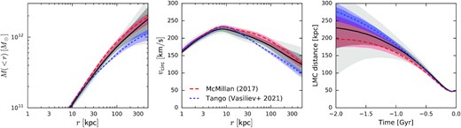
Results of DF fits with two tracer populations (clusters and satellites), taking into account the LMC perturbation. Left-hand panel shows the enclosed mass profile, centre panel – the corresponding circular velocity profile, and right-hand panel – the past LMC trajectory (distance from MW centre). Median values are plotted by black solid lines, dark and light-shaded regions show the 16/84 and 2.3/97.7 percentiles. For comparison, red-dashed lines and red-shaded region show the best-fitting potential and an ensemble of plausible potentials from McMillan (2017), the best-fitting potential being very close to the median potential in our series of models without the LMC. Likewise, blue short-dashed lines and blue-shaded region show the median and the ensemble of potentials from the Tango simulation (Vasiliev et al. 2021a), which was fit to the Sagittarius stream in the presence of the LMC.

Table 2.

Constraints on the MW mass profile at different radii from various combinations of tracers (globular clusters or satellites), with or without accounting for the LMC perturbation. We list the enclosed mass at 50, 100, and 200 kpc, as well as the virial mass (for the overdensity Δ = 102 w.r.t. the cosmological matter density). The last two rows are our preferred values from both data sets with orbit rewinding, using either the baseline Zhao halo profile or the alternative Einasto profile. Distances are given in kpc and masses – in |$10^{12}\, \mathrm{M}_\odot$|⁠, quoted as median and 16/84 percentiles.

	M(< 50)	M(< 100)	M(< 200)	M_vir
GC, no LMC	\|$0.51^{+0.12}_{-0.09}$\|	\|$0.79^{+0.33}_{-0.20}$\|	\|$1.08^{+0.69}_{-0.39}$\|	\|$1.2^{+1.0}_{-0.5}$\|
sat, no LMC	\|$0.50^{+0.07}_{-0.07}$\|	\|$0.85^{+0.12}_{-0.10}$\|	\|$1.31^{+0.29}_{-0.20}$\|	\|$1.6^{+0.6}_{-0.4}$\|
both, no LMC	\|$0.54^{+0.07}_{-0.06}$\|	\|$0.85^{+0.11}_{-0.09}$\|	\|$1.17^{+0.27}_{-0.23}$\|	\|$1.3^{+0.6}_{-0.3}$\|
both w/LMC	\|$0.45^{+0.04}_{-0.04}$\|	\|$0.73^{+0.09}_{-0.08}$\|	\|$1.10^{+0.27}_{-0.22}$\|	\|$1.3^{+0.6}_{-0.4}$\|
–’–, Einasto	\|$0.46^{+0.05}_{-0.04}$\|	\|$0.74^{+0.09}_{-0.07}$\|	\|$1.00^{+0.23}_{-0.17}$\|	\|$1.1^{+0.4}_{-0.3}$\|

	M(< 50)	M(< 100)	M(< 200)	M_vir
GC, no LMC	\|$0.51^{+0.12}_{-0.09}$\|	\|$0.79^{+0.33}_{-0.20}$\|	\|$1.08^{+0.69}_{-0.39}$\|	\|$1.2^{+1.0}_{-0.5}$\|
sat, no LMC	\|$0.50^{+0.07}_{-0.07}$\|	\|$0.85^{+0.12}_{-0.10}$\|	\|$1.31^{+0.29}_{-0.20}$\|	\|$1.6^{+0.6}_{-0.4}$\|
both, no LMC	\|$0.54^{+0.07}_{-0.06}$\|	\|$0.85^{+0.11}_{-0.09}$\|	\|$1.17^{+0.27}_{-0.23}$\|	\|$1.3^{+0.6}_{-0.3}$\|
both w/LMC	\|$0.45^{+0.04}_{-0.04}$\|	\|$0.73^{+0.09}_{-0.08}$\|	\|$1.10^{+0.27}_{-0.22}$\|	\|$1.3^{+0.6}_{-0.4}$\|
–’–, Einasto	\|$0.46^{+0.05}_{-0.04}$\|	\|$0.74^{+0.09}_{-0.07}$\|	\|$1.00^{+0.23}_{-0.17}$\|	\|$1.1^{+0.4}_{-0.3}$\|

Table 2.

Constraints on the MW mass profile at different radii from various combinations of tracers (globular clusters or satellites), with or without accounting for the LMC perturbation. We list the enclosed mass at 50, 100, and 200 kpc, as well as the virial mass (for the overdensity Δ = 102 w.r.t. the cosmological matter density). The last two rows are our preferred values from both data sets with orbit rewinding, using either the baseline Zhao halo profile or the alternative Einasto profile. Distances are given in kpc and masses – in |$10^{12}\, \mathrm{M}_\odot$|⁠, quoted as median and 16/84 percentiles.

	M(< 50)	M(< 100)	M(< 200)	M_vir
GC, no LMC	\|$0.51^{+0.12}_{-0.09}$\|	\|$0.79^{+0.33}_{-0.20}$\|	\|$1.08^{+0.69}_{-0.39}$\|	\|$1.2^{+1.0}_{-0.5}$\|
sat, no LMC	\|$0.50^{+0.07}_{-0.07}$\|	\|$0.85^{+0.12}_{-0.10}$\|	\|$1.31^{+0.29}_{-0.20}$\|	\|$1.6^{+0.6}_{-0.4}$\|
both, no LMC	\|$0.54^{+0.07}_{-0.06}$\|	\|$0.85^{+0.11}_{-0.09}$\|	\|$1.17^{+0.27}_{-0.23}$\|	\|$1.3^{+0.6}_{-0.3}$\|
both w/LMC	\|$0.45^{+0.04}_{-0.04}$\|	\|$0.73^{+0.09}_{-0.08}$\|	\|$1.10^{+0.27}_{-0.22}$\|	\|$1.3^{+0.6}_{-0.4}$\|
–’–, Einasto	\|$0.46^{+0.05}_{-0.04}$\|	\|$0.74^{+0.09}_{-0.07}$\|	\|$1.00^{+0.23}_{-0.17}$\|	\|$1.1^{+0.4}_{-0.3}$\|

	M(< 50)	M(< 100)	M(< 200)	M_vir
GC, no LMC	\|$0.51^{+0.12}_{-0.09}$\|	\|$0.79^{+0.33}_{-0.20}$\|	\|$1.08^{+0.69}_{-0.39}$\|	\|$1.2^{+1.0}_{-0.5}$\|
sat, no LMC	\|$0.50^{+0.07}_{-0.07}$\|	\|$0.85^{+0.12}_{-0.10}$\|	\|$1.31^{+0.29}_{-0.20}$\|	\|$1.6^{+0.6}_{-0.4}$\|
both, no LMC	\|$0.54^{+0.07}_{-0.06}$\|	\|$0.85^{+0.11}_{-0.09}$\|	\|$1.17^{+0.27}_{-0.23}$\|	\|$1.3^{+0.6}_{-0.3}$\|
both w/LMC	\|$0.45^{+0.04}_{-0.04}$\|	\|$0.73^{+0.09}_{-0.08}$\|	\|$1.10^{+0.27}_{-0.22}$\|	\|$1.3^{+0.6}_{-0.4}$\|
–’–, Einasto	\|$0.46^{+0.05}_{-0.04}$\|	\|$0.74^{+0.09}_{-0.07}$\|	\|$1.00^{+0.23}_{-0.17}$\|	\|$1.1^{+0.4}_{-0.3}$\|

As mentioned earlier, the flexibility of the Zhao density profile means that not all of its parameters can be usefully constrained by observations, and consequently the extrapolation of the halo density profile to larger radii (and thus the inferred virial mass) depend on the allowed range of shape parameters α and β. Supplementary data contain the covariance plots between the potential parameters used in the fit and the enclosed masses at different radii (50, 100, and 200 kpc and M_vir). We find that the outer slope β most significantly affects the virial mass, and to a slightly lesser extent M(< 200), with M_vir at the lower end of the allowed range of β (2.1) being 0.1 dex (i.e. 25 per cent) higher than at β = 3. Nevertheless, the mean likelihoods of models restricted to the range β ≥ 3 is the same as for the entire range of β; thus we cannot say that there is any real preference for lower β warranted by the data. We also examined an alternative family of Einasto profiles and found that they generally have more steeply falling density at large radii, and consequently lower virial masses (but still compatible with Zhao models within uncertainties). We conclude that in absence of more selective priors on the halo density profile, we cannot constrain the total MW mass to better than a factor of two; however, the enclosed mass at r ≲ 200 kpc is better constrained for any choice of halo model, and exhibits a systematic difference of |$\sim 15{{\ \rm per\ cent}}$| between the models with and without the LMC.

The median circular velocity curve in the fiducial Zhao series of models lies roughly halfway between the commonly used ‘best-fitting model’ for the MW potential by McMillan (2017) and the potential from the ‘Tango simulation’ (Vasiliev et al. 2021a), which was fit to the properties of the Sagittarius stream in the presence of the LMC perturbation. Both reference models have considerable uncertainties, which are often overlooked in the case of McMillan’s potential. The difference between these two is more pronounced at large radii, and results in a qualitative difference in the inferred past orbit of the LMC (right-hand panel of Fig. 5): while in the Tango simulations the LMC was nearly always on the first approach to the MW, in the heavier McMillan’s potential its past trajectory would have an apocentre distance ≲ 200 kpc and a period ∼3 Gyr. The LMC orbits in our series of fits typically have a longer period (4–6 Gyr) and larger apocentre distance, but |$\sim 90{{\ \rm per\ cent}}$| of them are still bound to the MW (i.e. had at least one additional pericentre passage in the last 7 Gyr). However, there is a strong evidence that the LMC is on its first encounter with the MW (e.g. Kallivayalil et al. 2013, and references therein). This argument alone implies a relatively light MW, on the lower end of our inferred mass range, though we caution that these models do not take into account that the MW mass was likely lower in the past, resulting in a less bound LMC trajectory for the same present mass (see fig. 11 in Kallivayalil et al. 2013). The gradual increase of the MW mass due to cosmological accretion of matter over many Gyr would not invalidate the DF fitting approach, since the orbital actions are conserved under slow variation of potential. Thus it is possible that the current MW mass lies in the range preferred by our fits, but the LMC is still on its first approach.

Our inferred MW mass profile agrees within uncertainties with various recent estimates (see Wang et al. 2020 for a compilation of results). Before Gaia DR2, very few satellites had PM measurements, and consequently the mass estimates varied widely between studies or even within a single study, but using different tracer subsets. For instance, Watkins et al. (2010), using a power-law mass estimator, found |$M(\lt 300) = (0.9\pm 0.3) \times 10^{12}\, \mathrm{M}_\odot$| using only line-of-sight velocities and assuming isotropy, or |$(0.7-3.4) \times 10^{12}\, \mathrm{M}_\odot$| under more general assumptions about anisotropy, while the sample of eight satellites (including LMC and SMC) with measured PM indicated a strong tangential anisotropy and hence implied |$M\gtrsim 2 \times 10^{12}\, \mathrm{M}_\odot$|⁠. The more recent PM measurements instead suggest only a mild tangential anisotropy for satellites, as discussed in the next section. With Gaia DR2 and HST measurements of satellite PM, and using the same power-law mass estimator, Fritz et al. (2020) measured |$M_\text{vir}=(1.5\pm 0.4) \times 10^{12}\, \mathrm{M}_\odot$|⁠, or |$M(\lt 100)=(0.8\pm 0.2) \times 10^{12}\, \mathrm{M}_\odot$|⁠. The choice of method may significantly affect the result: for instance, Eadie & Juric (2019), using the same catalogue of globular clusters as Vasiliev (2019b), but employing a variant of power-law mass estimator, determined |$M(\lt 100)=0.53^{+0.21}_{-0.12}\times 10^{12}\, \mathrm{M}_\odot$|⁠, almost 40 per cent lower than the latter study. Recently, Slizewski et al. (2022) applied the method of Eadie & Juric (2019) to the satellite tracers (still using PM from Gaia DR2) and found |$M(\lt 100)=(0.88\pm 0.1)\times 10^{12}\, \mathrm{M}_\odot$|⁠. On the other hand, Wang, Hammer & Yang (2022) used a nearly identical method to Vasiliev (2019b) with the updated Gaia EDR3-based PM measurements of globular clusters, and obtained a rather low virial mass |$0.83^{+0.36}_{-0.21}\times 10^{12}\, \mathrm{M}_\odot$| (quoted for the overdensity of 200; to compare with our definition, these values should be increased by |$\sim 16{{\ \rm per\ cent}}$|⁠) when using our PM measurements with the Zhao density profile, and even considerably smaller when using the Einasto profile. They additionally imposed tight constraints on the circular velocity at 5 < r < 25 kpc taken from Eilers et al. (2019), which are based on kinematics of stars in the Galactic disc. We repeated our analysis while imposing the same prior on the inner circular-velocity curve and got very similar results to Wang et al. (2022) when using only globular clusters; however, the fits to the combined data set of clusters and satellites instead yielded higher virial masses, more consistent with our default set-up (which does not use additional priors from stellar kinematics). As we do not expect that clusters alone can provide useful constraints for the enclosed mass at r ≳ 100 kpc, we tend to trust the combined fits more, but note that even these do not tightly constrain the virial mass without additional priors on the behaviour of halo density at large radii.

Since the assumption of virial equilibrium may be questionable for the satellite population, numerous studies instead estimated the MW mass by comparing the satellite distribution with cosmological simulations: in particular, Cautun et al. (2020) find |$M(\lt 100) = 0.65^{+0.08}_{-0.06}\times 10^{12}\, \mathrm{M}_\odot$|⁠, and Li et al. (2020a) find |$M(\lt 100) = (0.72\pm 0.1) \times 10^{12}\, \mathrm{M}_\odot$|⁠; these values are well compatible with our measurements. The MW mass profile may also be constrained by other dynamical tracers, such as distant halo stars or stellar streams. A recent study of Shen et al. (2022), using ∼170 stars from the H3 survey and the Eadie & Juric (2019) modelling method, measured |$M(\lt 100) = (0.69\pm 0.05)\times 10^{12}\, \mathrm{M}_\odot$|⁠, but noted that the simple power-law model cannot simultaneously fit well the density and velocity distribution of tracers. With a compilation of ∼500 MW halo stars from several surveys and again using a power-law mass estimator, Deason et al. (2021) found |$M(\lt 100) = 0.61 \pm 0.03\, \text{(stat.)} \pm 0.12\, \text{(sys.)} \times 10^{12}\, \mathrm{M}_\odot$|⁠, somewhat lower than we measure. Interestingly, although they approximately accounted for the LMC influence by adding a velocity offset to the measured values, this had very little effect on the results; their systematic uncertainty rather reflects the scatter in assembly histories of galaxies in cosmological simulations. Finally, we note that the ‘Tango’ MW + LMC model fitted to the Sagittarius stream (Vasiliev et al. 2021a) also has a lower mass: |$M(\lt 100) = (0.56 \pm 0.04) \times 10^{12}\, \mathrm{M}_\odot$|⁠. Nevertheless, these values are still within the 95 per cent confidence interval of models in this study (in particular, if we run our fits with a fixed Tango potential, varying only the parameters of tracer DFs, the log-likelihood is decreased by |$\Delta \ln \mathcal {L}\simeq 3$|⁠).

Although the inferred MW mass profile and the virial mass in models with or without LMC is compatible within uncertainties, the former produce materially better fits. The difference in log-likelihood is |$\Delta \ln \mathcal {L}\simeq 12$|⁠, split roughly equally between clusters and satellites: in other words, a non-zero LMC mass is preferred with high significance. Fig. 6 shows the posterior distribution of LMC mass values, which lies between 10¹¹ and |$2\times 10^{11}\, \mathrm{M}_\odot$| – same range as inferred from various independent pieces of evidence in recent works, e.g. perturbations to stellar streams (Erkal et al. 2019; Shipp et al. 2021; Vasiliev et al. 2021a), the census of its satellites (Erkal & Belokurov 2020; Battaglia et al. 2022), the requirement to gravitationally bind the SMC (Kallivayalil et al. 2013), and finally, the density and kinematic asymmetries in the MW stellar halo (Conroy et al. 2021; Erkal et al. 2021; Petersen & Peñarrubia 2021). The physical reason why our fits are able to constrain the LMC mass is illustrated by Fig. 7, which shows the measured z-component of velocities of satellite galaxies (for simplicity, without uncertainties). As clear from this plot and from a similar fig. 6 in Erkal et al. (2020), there is a significant kinematic asymmetry: the mean velocity is ∼60 km s⁻¹, with three quarters of objects having positive v_z. If we rewind their orbits back in time in the presence of the LMC perturbation, and then integrate forward up to present time in a static MW potential, almost all of them would have lower v_z, decreasing the mean value threefold. Since the DF fitting (or any other method based on the equilibrium assumption) implicitly assumes a uniform distribution in orbital phases, it naturally returns a higher likelihood for a more symmetric distribution of v_z, and since the dispersion of values also decreases, so does the inferred MW mass.

Figure 6.

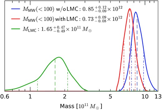
Posterior distribution of the enclosed MW mass at 100 kpc in models without LMC (blue) and with LMC rewinding (red), and the LMC mass in the latter series of models (green).

Figure 7.

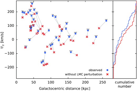
Illustration of the significant kinematic asymmetry in the satellite distribution induced by the LMC. Blue dots show the z-component of velocity plotted against Galactocentric distance for the 36 satellites selected for the fit; three quarters of them have v_z > 0, with a mean value of 60 km s⁻¹ for the entire population (see also fig. 6 in Erkal et al. 2020). Red crosses show the same quantities that these object would have in absence of the LMC perturbation, obtained by integrating the present-day positions and velocities backward in time for 2 Gyr in the time-dependent MW + LMC potential and then integrating them forward in the static MW-only potential. Almost all galaxies would have had lower v_z in this case, bringing the overall distribution closer to symmetry (compare the cumulative distributions in the right-hand panel) with a mean v_z of only 20 km s⁻¹.

5.2 Properties of tracer populations

As a by-product of our fits, we can also examine the properties of the tracer DFs manifested as the density and velocity dispersion profiles. Fig. 8 shows both populations on the same scale: they are clearly separated in radius by more than a factor of 10, which is beneficial for the determination of the potential, as discussed in Walker & Peñarrubia (2011). The density profiles (left-hand panel) are well approximated by a Spheroid model (equation 4) with parameters listed in Table 1, though both populations are non-spherical (clusters are more oblate in the inner Galaxy, and satellites are slighly prolate, as shown in the right-hand panel). Their kinematic properties are also quite different: although both are moderately rotating in central parts (v_ϕ ∼ 50–70 km s⁻¹, see e.g. Frenk & White 1980 for an early analysis of cluster kinematics), clusters are close to isotropic in the inner Galaxy and become significantly radially anisotropic further out, with σ_r/σ_{{θ, ϕ}} ≃ 2, whereas for satellites, σ_r lies between σ_ϕ and σ_θ, with a mild tangental anisotropy. However, we caution that these properties are determined by the DF under the assumption of dynamical equilibrium. If we instead fit simple parametric density and velocity dispersion profiles to the actual satellite catalogue, without linking them to each other in any way, the spatial distribution of objects is significantly more extended in the z direction, with axial ratio z/R closer to two, but the velocity anisotropy changes from mildly tangential in the inner part to nearly isotropic or even weakly radially dominated in the outer part (see e.g. Riley et al. 2019). These two properties apparently cannot be reconciled in a steady-state model, hence the configuration represented by the DF is a trade-off between these conflicting requirements, and neither the shape nor the velocity anisotropy resemble the present-day configuration particularly well.

$Properties of the two tracer populations: globular clusters (solid lines) and satellites (dashed lines). Left-hand panel shows the sphericalized 3D density multiplied by r3, i.e. the number of objects per logarithmic interval of radii (normalized to unity for each population; the actual number of objects used in the fit is 154 clusters and 36 satellites). Centre panel shows the three components of velocity dispersion in spherical coordinates, and the mean rotation velocity. Right-hand panel shows the velocity anisotropy coefficient $\beta \equiv 1 - (\sigma _\theta ^2 + \sigma _\phi ^2) / (2 \sigma _r^2)$ and the axial ratio z/R of the axisymmetric density profile: clusters are flattened in the central part of the Galaxy and more spherical in the outer part, while satellites have a slightly prolate distribution overall. Lines show the median and shaded regions – 16/84 percentiles in the MCMC ensemble of models.$

Figure 8.

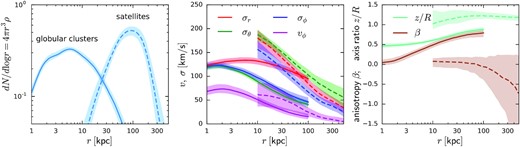
Properties of the two tracer populations: globular clusters (solid lines) and satellites (dashed lines). Left-hand panel shows the sphericalized 3D density multiplied by r³, i.e. the number of objects per logarithmic interval of radii (normalized to unity for each population; the actual number of objects used in the fit is 154 clusters and 36 satellites). Centre panel shows the three components of velocity dispersion in spherical coordinates, and the mean rotation velocity. Right-hand panel shows the velocity anisotropy coefficient |$\beta \equiv 1 - (\sigma _\theta ^2 + \sigma _\phi ^2) / (2 \sigma _r^2)$| and the axial ratio z/R of the axisymmetric density profile: clusters are flattened in the central part of the Galaxy and more spherical in the outer part, while satellites have a slightly prolate distribution overall. Lines show the median and shaded regions – 16/84 percentiles in the MCMC ensemble of models.

In fact, these features are likely caused by a spatially and kinematically coherent feature known as the Vast Polar Structure (VPOS; e.g. Kroupa, Theis & Boily 2005, Pawlowski & Kroupa 2020), roughly perpendicular to the Galactic disc. We recall that we excluded the LMC and its likely satellites from the sample, but even the remaining galaxies have a significantly anisotropic distribution of orbital poles, as illustrated in Fig. 9, left-hand panel. It has been suggested by Garavito-Camargo et al. (2021b) that the gravitational effect of the LMC may cause or enhance the orbital pole clustering. However, if we ‘undo’ the LMC perturbation in the same way as for v_z, i.e. rewinding orbits in a time-dependent MW + LMC potential and then bringing them back to present time in a static MW potential, the resulting distribution of orbital poles does not significantly change (right-hand panel) and still remains rather non-uniform; thus the LMC perturbation cannot be the main cause of the orbital pole clustering (the same conclusion is independently reached by Pawlowski et al. 2021). Li et al. (2021) estimated that around a half of the entire satellite population may be part of VPOS, including the LMC itself and its satellites.

Figure 9.

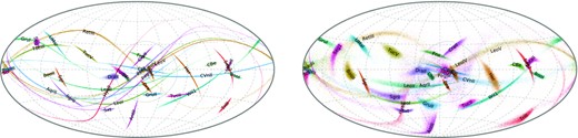
Orbital poles of selected satellite galaxies (excluding the LMC and its likely satellites), shown on the celestial sphere in the same coordinates as fig. 3 in Fritz et al. (2018) or fig. 2 in Li et al. (2021). Each object is shown by a cloud of points representing its posterior distribution of phase-space coordinates, with distance uncertainty usually the dominant one (hence the clouds are stretched along great circles). Left-hand panel shows the actual present-day measurements, right-hand panel – the orientation of orbital poles that the objects would have if not perturbed by the LMC. The angular momentum direction of the MW disc is at the bottom of this sphere, and the largest concentration of orbital poles is around the VPOS, marked by a grey circle in the centre, which is roughly orthogonal to the MW disc.

In the above figure and in subsequent ones, each object is rendered as a cloud of points representing the uncertainty in its orbit parameters, which stems both from the measurement uncertainties and from the variation in the potential in our ensemble of models (including the LMC mass). However, it is important to stress that one should not sample uniformly from the measurement error distribution, but rather from the posterior distribution (i.e. weighted by the DF value). As a simple illustration, consider an object moving on a nearly circular orbit at a certain radius, and imagine that its PM is measured with a relatively large uncertainty comparable to the value itself. Then most samples from this error distribution will produce a higher velocity and hence place the object at the pericentre of an eccentric orbit with a larger apocentre radius, or even on an unbound orbit. Thus, if one assigns equal probability to all these samples, one would arrive at an incorrect conclusion that the object is likely near the pericentre of a highly eccentric orbit. If, on the other hand, one accounts for the fact that lower velocity corresponding to a more tightly bound orbit is more likely to be found among the ensemble of all orbits generated by the DF, the inference will be unbiased. This resolves the apparent ‘double convolution’ paradox: assuming that we have a given intrinsic distribution of some quantity (say, velocity), and that measured values are equally likely to be smaller or larger than the true value for any object, the observed distribution will be broadened by errors. Now, by sampling from a Gaussian error distribution around the measured value, we effectively broaden the true distribution a second time, but by assigning higher weight to samples that have smaller velocities, we may recover the true width of the intrinsic distribution, and the posterior distribution of possible true velocity values for each object will be shifted towards lower-than-measured values. Of course, this requires a model for the intrinsic distribution to be constructed from the measured values, which is precisely what we do in our fits. A caveat is that if the model contains only the equilibrium DF in the given potential, all posterior orbits will necessarily be gravitationally bound to the MW. However, since we introduced a second, ‘unmixed’ population of object containing both positive and mildly negative energies, we do not artificially enforce the orbits to be bound.

To construct our posterior sample of orbit parameters |$\boldsymbol{w}_i$| for the i-th object, we first draw samples |$\boldsymbol{w}_i^{(s)}, s=1..N_\text{samp}$| from the Gaussian error distribution of this object. Then we iterate over a large number of model parameters from the MCMC ensemble, and for each model m of the potential and the DF |$f_m(\boldsymbol{w})$|⁠, evaluate the likelihood of all samples:

$$\begin{eqnarray*} f_m \left(\boldsymbol{w}_i^{(s)}\right),\quad s=1..N_\text{samp}\, , \end{eqnarray*}$$

(14)

then pick up one or more samples with probability

$$\begin{eqnarray*} p_i^{(s)} \equiv \frac{f_m \left(\boldsymbol{w}_i^{(s)} \right)}{\sum _{s^{\prime }=1}^{N_\text{samp}} f_m \left(\boldsymbol{w}_i^{(s^{\prime })} \right)} \, , \end{eqnarray*}$$

(15)

and finally stack together the posterior samples from all examined models (note that the denominator in the above equation is the error-convolved DF value as in equation (7)). For the majority of objects, the posterior distribution averaged over many models in the MCMC ensemble is actually very close to a normal distribution centred on the measured values with quoted uncertainties, i.e. the measurement errors are effectively negligibly small. One may quantify the reduction in the posterior width by the entropy, defined as

$$\begin{eqnarray*} S_i \equiv -\!\!\sum _{s=1}^{N_\text{samp}} p_i^{(s)}\,\, \ln \left (p_i^{(s)}\, N_\text{samp}\right) \le 0. \end{eqnarray*}$$

(16)

If the measurement errors are small, all |$p_i^{(s)}$| are close to 1/N_samp, and hence the entropy is close to zero; if a single sample dominates the sum, S ≈ −ln N_samp. Objects with the largest negative entropy show the largest reduction in the posterior width, and unsurprisingly, typically have relatively large PM uncertainties or no line-of-sight velocity measurements. These include a few faint globular clusters, namely, Crater, AM 1, AM 4, and Muñoz 1: the first two are also the most distant ones, while the latter two are very faint clusters at distances ∼30 and ∼45 kpc, respectively, which have no stars on the giant branch. Among satellite galaxies with S < −0.5 are Columba I, Eridanus II, Hydra II, Leo IV, Leo V, Pegasus III, Pisces II, Reticulum III (most of them are rather distant), and some (but not all) objects with no line-of-sight velocities: Boötes IV, Cetus II, Cetus III, Indus I, and Pictor I.

In a mixture model for the satellite sample, we additionally evaluate the posterior probability of belonging to the unmixed (infalling, splashback, and unbound) population for each object (equation 12). It turns out that in models without the LMC, Leo I has a high probability of being unmixed, which is not surprising, given its high velocity and large distance. However, when accounting for the LMC perturbation, its pre-LMC orbit actually has a lower energy and is likely to belong to the main sample, except if the MW mass is small enough (⁠|$M_\text{vir}\lesssim 0.9\times 10^{12}\, \mathrm{M}_\odot$|⁠). Hercules, on the other hand, is confidently bound in all models without LMC, but also has a significant probability of being unmixed in a low-mass MW + LMC scenario. Although the mixture model is much less sensitive to an occasional outlier than a standard model with only bound population, we repeated the fits excluding these two galaxies from the sample. The inferred mass within 100 kpc was |$\sim 10{{\ \rm per\ cent}}$| lower in this case, but well within uncertainties of the fiducial scenario. We also looked at the probability of belonging to the unmixed population for other objects not included in the main sample. Apart from the likely LMC satellites, which are examined in the next section, the following objects were found not to be among virialized satellites: Columba I, Eridanus II, Leo T, and Phoenix (which are all distant and still infalling), and possibly Cetus III and Boötes IV (which have no line-of-sight velocity measurements).

With the posterior samples, we construct the diagram of orbital phases of satellite galaxies: for each choice of potential and each sample from the position/velocity distribution, we compute the radial phase angle θ_r – a canonically conjugate variable to the radial action, which uniformly increases with time. A well-mixed population is expected to have a uniform distribution of θ_r. Fig. 10 shows the 36 galaxies from the main data set used in the fit, plus a few objects with poor PM measurements that were excluded from the sample (Pegasus III, Pisces II, and Ridiculum III). This plot does not include the LMC itself, its likely satellites, and objects with high posterior probability of belonging to the unmixed population or without line-of-sight velocities. We observe that there is no significant bias towards close-to-pericentre orbital phases, in contrast to the analyses of Simon (2018), Fritz et al. (2018), and Li et al. (2021), which, however, used raw measurements rather than posterior distribution, possibly leading to a bias as explained above. The inclusion of the LMC does not significantly change this distribution (we again perform a backward-then-forward rewinding to undo the LMC perturbation, but caution that the reconstruction of angle variables may be less accurate than the integrals of motion).

Figure 10.

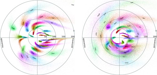
Distribution of satellites in the space of energy and orbital phase. In the polar coordinates, radius corresponds to the radius of a circular orbit with the given energy, and polar angle – the radial phase angle θ_r; each galaxy is rendered by a cloud of points sampling from the joint posterior distribution of MW and LMC potential models and measurement uncertainties. Only a subset of all satellites is shown, excluding the galaxies associated with the LMC and a few likely non-virialized objects. Left-hand panel shows the ensemble of models without the LMC, so that the location of points corresponds to the actual present-day phase-space coordinates of these objects. Right-hand panel depicts the ensemble of models with the LMC: the energy and orbital phase are obtained by integrating orbits backward from the present-day coordinates in the time-dependent MW + LMC potential, and then integrating forward to present time in a static MW potential, thus the scatter of points is increased by the variation in the MW potential parameters.

However, we caution that the DF fitting method (or any other approach invoking the Jeans theorem) implicitly assumes a uniform distribution in angle space, and hence prefers potentials that make the observed population consistent with uniform random sampling of orbital phases. If the MW mass were lower, the same measured velocities of objects would be relatively larger compared to the equilibrium velocity distribution at a given radius, and hence one would infer that many of the objects are near the pericentres of their orbits. However, since there is no corresponding population of more distant and slower objects near their apocentres, this potential would be assigned a lower likelihood in the model. On the other hand, if there actually exist distant undiscovered satellites (for instance, Koposov et al. 2008 estimate that up to 50–100 faint satellites are still undetected), the inferred MW potential would need to be revised downwards, as illustrated by a toy experiment in the appendix.

We now examine more systematically the effect of the LMC on the orbits of clusters and satellite galaxies, using the posterior samples in two MCMC ensembles of models, with and without orbit rewinding. As expected, we do not find any significant changes in cluster orbits with or without the LMC, in agreement with Garrow, Webb & Bovy (2020), nor are any cluster orbits associated with the LMC, confirming Boldrini & Bovy (2021); thus we concentrate on the satellites in what follows. Fig. 11 shows the time evolution of Galactocentric distance over the last 3 Gyr⁵ for models without LMC in blue, and with LMC in red. Green lines additionally show the evolution of orbit energy with respect to its current value in the latter series of models: if it stays around zero, the LMC has little effect on the orbit, but it can also be larger in the past (i.e. the galaxy was moved by the LMC on to a more tightly bound orbit) or vice versa. We observe that for some objects (e.g. Segue 1 or Willman 1), especially in the inner Galaxy, the red and the blue series of orbits are rather similar, but for the majority of them, the orbits look quite different. There are, of course, satellites of the LMC, which have been affected by it over the entire time interval, as evidenced by the large spread of green curves (e.g. Carina III or Hydrus I); we discuss them in more detail in the next section. For others, the influence of the LMC is mainly limited to the last 0.5 Gyr. We stress that this need not be a direct gravitational scattering by the LMC itself (though this likely happened for Aquarius II, Grus II, Sagittarius II, Tucana III, Tucana IV, and Tucana V), but rather the change in MW-centric orbit parameters as a result of the MW reflex motion caused by the LMC. As illustrated by Fig. 3, objects beyond a few tens kpc are likely to be moved up or down in energy, but the former occurs more often. For some galaxies, this dramatically alters their inferred past orbit; a prime example is Leo I, which had a more tightly bound orbit in the past until the arrival of the LMC, as already noted by Erkal et al. (2020, their section 3.2). A similar conclusion is reached for Leo V, Sextans, and Tucana II. On the other hand, a surprisingly large fraction of satellites have been moved to more tightly bound orbits recently, including Canes Venatici II, Draco, Fornax, Hercules, Sculptor, and Ursa Minor. We note that in absence of any energy change (e.g. Crater II or Ursa Major I), orbits in the series of models with LMC would be somewhat larger than in models without LMC, on account of a lower MW mass in the former case, but the difference in orbits for the above named galaxies is far more pronounced. Among them, only Hercules is affected to such an extent that it might have been on a splashback orbit prior to the LMC-induced perturbation, but the orbits of Carina and Sculptor are also dramatically changed and had a higher eccentricity in the past. We note that the orbit of Sagittarius dSph also increased its eccentricity due to the LMC perturbation (see fig. 9 in Vasiliev et al. 2021a), but these changes are still minor compared to what many other satellites have experienced. It is clear that the LMC cannot be neglected when analysing the past trajectories, tidal forces, and mass loss history of most MW satellites.

Figure 11.

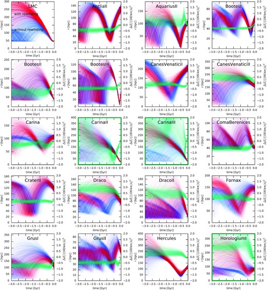
Orbits of satellite galaxies in the models neglecting the LMC (blue) or including it (red). For each object, we show the evolution of the Galactocentric radius for a variety of orbits integrated in different potentials with parameters drawn from the MCMC ensemble of models, and the orbital initial conditions (present-day positions and velocities) drawn from the posterior distribution of each model (i.e. are sampled from measurement uncertainties and weighted with the probability of each sample in the given DF and potential model). The top left panel shows the trajectories of the LMC itself (neglecting observational uncertainties). In the remaining panels, cyan lines additionally show the evolution of energy for each orbit with respect to its present-day value (secondary axis) for the case of the time-dependent MW + LMC potential. When the energy does not change significantly (e.g. for Crater II or Fornax), the orbits in the time-dependent potential are somewhat more extended since the MW is on average less massive in this series of models. But the recent LMC-induced energy kicks may be both positive or negative and can significantly alter the inferred orbits (e.g. for Carina or Grus I), or the object might end up being bound to the LMC over its past orbit, in which case the energy in the MW potential varies wildly (e.g. Carina III).

Figure 11.

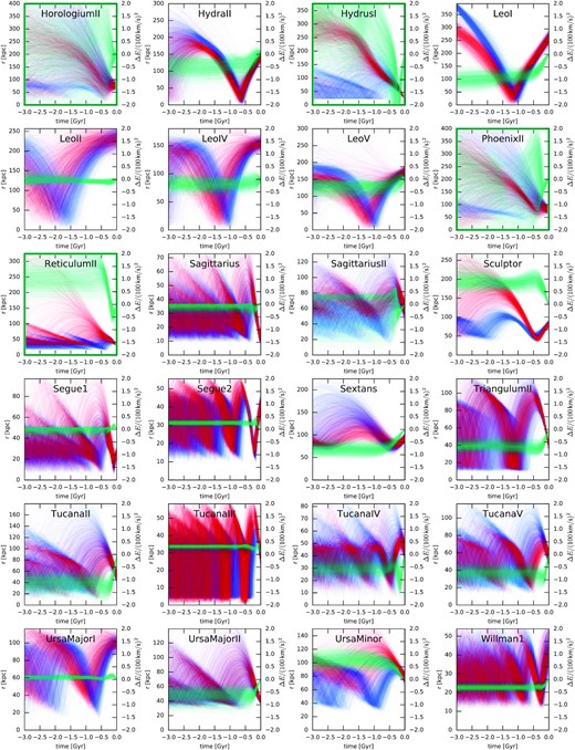
Continued.

5.3 Satellites of the LMC

We now turn attention to the objects suspected to be LMC satellites and therefore excluded from the main sample during the fit (marked by green frames in Fig. 11). Their past orbits in models with the LMC are indeed concentrated around the past trajectory of the LMC itself, and their energy in the MW-centred frame has large fluctuations at all times, not just over the last 0.5 Gyr. For a better view, Fig. 12 shows the evolution of the distance from the LMC for these and a few other galaxies, and the evolution of energy in the LMC-centred frame E_LMC (i.e. using the relative velocity). Although this energy may change rather dramatically in the last 0.5 Gyr due to the complex three-body interaction between the MW, the LMC, and the satellite galaxy, it often ends up being negative for a large fraction of orbits (recall that the ensemble of orbits encompasses the uncertainties in the current coordinates, MW potentials and LMC masses, but in this case we do not additionally reweigh orbits by their posterior probability in the MW-bound DF).

$History of interaction with the LMC for selected galaxies over the past 3 Gyr. For each object, red lines show the distances from the LMC as a function of time for an ensemble of orbits sampled from the uncertainties in the present-day position/velocity, variations in the MW potential, and the LMC mass; cyan lines show the relative energy w.r.t. the LMC (ignoring the MW). A substantial fraction of green lines below zero indicates that the object is likely to be an LMC satellite (though it might not be bound at present time): this is the case for the galaxies in the first two rows, though Horologium II and Reticulum II have only a moderate overall probability of being bound in the past. The galaxies in the third row lack line-of-sight velocity measurements, but could have been bound to the LMC for a range of possible velocities. The last two rows show galaxies that have experienced a close passage with the LMC recently, but were not bound to it earlier, and with a possible exception of Grus II and Tucana IV, are unlikely to be bound at present time.$

Figure 12.

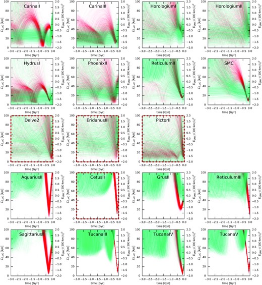
History of interaction with the LMC for selected galaxies over the past 3 Gyr. For each object, red lines show the distances from the LMC as a function of time for an ensemble of orbits sampled from the uncertainties in the present-day position/velocity, variations in the MW potential, and the LMC mass; cyan lines show the relative energy w.r.t. the LMC (ignoring the MW). A substantial fraction of green lines below zero indicates that the object is likely to be an LMC satellite (though it might not be bound at present time): this is the case for the galaxies in the first two rows, though Horologium II and Reticulum II have only a moderate overall probability of being bound in the past. The galaxies in the third row lack line-of-sight velocity measurements, but could have been bound to the LMC for a range of possible velocities. The last two rows show galaxies that have experienced a close passage with the LMC recently, but were not bound to it earlier, and with a possible exception of Grus II and Tucana IV, are unlikely to be bound at present time.

To quantify the probability of being an LMC satellite, we use the fraction of orbits with E_LMC < 0 over the time interval between −3 and −1 Gyr. Fig. 13 shows this fraction as a function of the LMC mass and a second parameter – either the heliocentric distance or the line-of-sight velocity. We find that Carina II, Carina III, Horologium I, Hydrus I, Phoenix II, and SMC have high probability of being bound to the LMC in the past regardless of the LMC mass (though it generally increases with mass), at least in most of the range of heliocentric distances compatible with observations. Reticulum II has a lower probability overall, unless its distance is underestimated (typically it would be bound for D ≳ 35 kpc for |$M_\text{LMC} \ge 10^{11}\, \mathrm{M}_\odot$| or D ≳ 33 kpc for |$M_\text{LMC} \ge 2\times 10^{11}\, \mathrm{M}_\odot$|⁠, while the observed distance is 31.6 ± 1.5 kpc). Horologium II also has a large spread in probabilities at all LMC masses, possibly due to relatively large PM uncertainties.

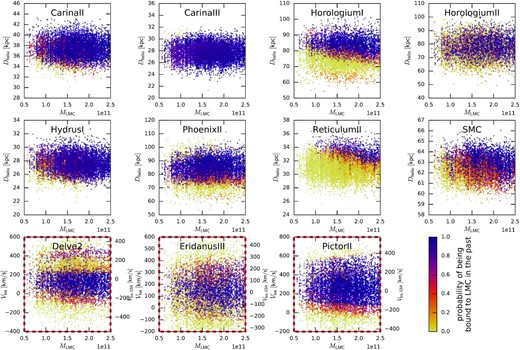
$Probability of past association with the LMC for selected galaxies. Each point represents an orbit sampled from the uncertainties in the present-day position/velocity, variations in the MW potential, and the LMC mass (without posterior reweighting); the colour indicates the fraction of time that this orbit had a negative energy w.r.t. LMC in the interval between −3 and −1 Gyr in the past. Orbits are plotted against LMC mass and either the heliocentric distance (top two rows) or the presently unknown line-of-sight velocity (bottom row).$

Figure 13.

Probability of past association with the LMC for selected galaxies. Each point represents an orbit sampled from the uncertainties in the present-day position/velocity, variations in the MW potential, and the LMC mass (without posterior reweighting); the colour indicates the fraction of time that this orbit had a negative energy w.r.t. LMC in the interval between −3 and −1 Gyr in the past. Orbits are plotted against LMC mass and either the heliocentric distance (top two rows) or the presently unknown line-of-sight velocity (bottom row).

10.1051/0004-6361/202141528

In addition, we find a few LMC satellite candidates among objects with no line-of-sight velocity measurements, shown in the third row of Figs 12 and 13. Pictor II, Delve 2, and Eridanus III are currently located within 10, 30, and 40 kpc from the LMC, respectively, but their PM are compatible with the past association with the LMC (marginally, in the case of Eridanus III). Naturally, this is conditioned on the currently unknown velocity, namely: v_los needs to be 110 ± 80 km s⁻¹ for Delve 2, 200± 70 km s⁻¹ for Eridanus III, or 270 ± 120 km s⁻¹ for Pictor II. The association between these objects and the LMC has been previously proposed in Cerny et al. (2021), Kallivayalil et al. (2018), Erkal & Belokurov (2020), and Drlica-Wagner et al. (2016), with similar predictions for the missing velocity.

Galaxies shown in the lower two rows of Fig. 12 had a close passage with the LMC in the last few hundred Myr, but were not among its satellites in the past. Two of them (Grus II and Tucana IV) currently may have velocities below the escape velocity of the LMC, but might not remain bound in the future on account of strongly dynamic interactions with both the LMC and the MW. For the remaining galaxies, we do not find any significant probability of LMC association in the past, although some of the brightest satellites (e.g. Carina, Fornax) share the orbital plane with the LMC and might be accreted from the same filament on cosmological timescales (e.g. Pardy et al. 2020).

Our assessment of the LMC satellite population broadly agrees with other studies (Jethwa et al. 2016, Kallivayalil et al. 2018, Erkal & Belokurov 2020, Patel et al. 2020, Battaglia et al. 2022), which typically limited their analysis to one or a few choices of MW potential. For Carina II, Carina III, Horologium I, Hydrus I, and SMC there is a general concensus that they have been associated with (a massive enough) LMC in the past. Horologium II, Phoenix II, and Reticulum II are more debatable; we find respectively moderate, high, and low probability of them being former LMC satellites.

6 DISCUSSION AND CONCLUSIONS

The role of the LMC as a major factor affecting the dynamics in the outer reaches of our Galaxy is gradually becoming appreciated by the community, but the tools for incorporating this factor into analysis are still scarce. Here, we introduced a simple but effective approach for ‘restoring order’ by first computing the past orbits of the MW and the LMC under mutual gravity, and then rewinding the orbits of stars or any other MW-bound objects in a time-dependent potential of the two galaxies, thus reconstructing the unperturbed state of the MW before the arrival of the LMC. This opens up the possibility to apply well-developed classical methods for dynamical modelling and measurement of gravitational potential based on the equilibrium approximation.

We then invoked one such method, simultaneously constraining the tracer DF, the MW potential, and the LMC mass, using two complementary data sets of objects with 6D phase-space coordinates: globular clusters and satellite galaxies. We demonstrated that the method is able to recover the true potential in the presence of the LMC perturbation, and that the neglect of this perturbation biases the inferred MW mass up by ∼20 per cent, in agreement with estimates by Erkal et al. (2020). Applying our method to the most recent measurements based on Gaia EDR3, we measured the MW mass distribution up to the virial radius with a relative uncertainty of |$\sim 20{{\ \rm per\ cent}}$| at 200 kpc (see Table 2), although we do not obtain tight constraints on the virial mass. The most likely range for the LMC mass is |$(1\!-\!2)\times 10^{11}\, \mathrm{M}_\odot$|⁠; models without the LMC perturbation are noticeably worse in fitting the observed data set (the difference in log-likelihood is ∼12).

We stress that the effect of the LMC cannot be simply reduced to a deflection of orbits that pass close to it. Equally, if not more important, is the reflex motion of the central region of the MW in response to the LMC’s gravitational pull, displacing it spatially and kinematically w.r.t. the outer part. The more distant objects are not able to keep up with this recent swinging motion of the MW-centred reference frame, and thus find themselves on significantly different orbits than without the LMC perturbation: this is clearly manifested in the energy variations in the last 0.5 Gyr in a large fraction of satellite galaxies (green curves in Fig. 11) and the corresponding differences in inferred past orbits with and without the LMC (red and blue curves in that figure). Nevertheless, the global features of the entire population of satellites, such as the orientations of angular momentum vectors (Fig. 9) or distribution of orbital phases (Fig. 10), are robust w.r.t. the inclusion of the LMC.

In contrast to some other studies (e.g. Fritz et al. 2018, Li et al. 2021), we do not find any evidence for a concentration of satellites near the pericentres of their orbits, nor for a strong tangential anisotropy of their velocities. We stress that this assessment is based on the limited selection of galaxies that does not include the LMC and its likely satellites, which are, of course, mostly near their pericentres, but should not count as independent samples. However, there are two further reasons for our different conclusion. One is that we use posterior-weighted uncertainties rather than raw measurements, which downweights the high-velocity tail of the observational error distribution. The other is that since we let the potential vary in the fit, the models choose the MW mass profile that prefers a more uniform distribution of orbital phases by construction. Nevertheless, we highlight a possible caveat in this line of reasoning: if the observed catalogue of satellites is incomplete and there exist yet undiscovered objects at large distances (hence more likely to be at apocentres), our inference on the MW mass would be biased up, as illustrated in the appendix, and in the true (lower-mass) potential, the observed distribution of satellites should indeed be concentrated near pericentres. If the selection function of the observed sample could be reliably estimated, this effect may be taken into account in our modelling scheme, as illustrated e.g. by Hattori et al. (2021) in a similar context.

Inevitably, our approach has a number of limitations. For simplicity, we neglect the measurement uncertainties on the LMC position and velocity, which are fairly small compared to uncertainties of many other objects. We also ignore the gravitational interaction between LMC and SMC, which might deflect the LMC and thus affect its past orbit reconstruction. More fundamentally, we assume a fixed (non-deforming) potential of both MW and LMC; note that the deformation of the tracer density profile is implicitly accounted for by the orbit rewinding procedure. Nevertheless, even this rather simplified reconstruction of the LMC orbit is able to compensate, in the first approximation, its perturbation on MW tracers.

The orbit rewinding step can be easily added to any forward-modelling approach constrained by kinematics of individual tracers, such as halo stars or tidal streams. Thus the significant gravitational perturbation from the LMC does not invalidate the classical dynamical modelling tools, but should be taken into account if we aim for a 10 per cent accuracy level that matches the quality of modern observational data sets.

SUPPORTING INFORMATION

supplementary_material.pdf

Covariance plots for potential parameters.

Please note: Oxford University Press is not responsible for the content or functionality of any supporting materials supplied by the authors. Any queries (other than missing material) should be directed to the corresponding author for the article.

ACKNOWLEDGEMENTS

We thank V. Belokurov, D. Erkal, W. Evans, and S. Koposov for valuable discussions, and the anonymous referee for expedient and comprehensive reports, which prompted us to extend our analysis and clarify various issues, improving the presentation. EV acknowledges support from STFC via the Consolidated grant to the Institute of Astronomy.

Software used: numpy, matplotlib, emcee (ascl:1303.002), gyrfalcon (ascl:1402.031), and nemo (ascl:1010.051).

DATA AVAILABILITY

We provide samples of the MW and LMC potential parameters from our MCMC analysis and corresponding satellite orbits, together with example python scripts for orbit rewinding, at the following repository: https://zenodo.org/record/5541971.

Footnotes

1

Here, r_vir is defined as the radius within which the mean density is 102 times higher than the cosmic density of matter, and is related to the virial mass as |$r_\text{vir} = (M_\text{vir}/10^{12}\, \mathrm{M}_\odot)^{1/3} \times 260$| kpc.

2

The velocity dispersion could be obtained from the Jeans equation for each choice of MW potential, but for simplicity, we adopt a universal profile |$\sigma _\text{MW} = 150 / \big (1 + |\boldsymbol{x}_\text{LMC}-\boldsymbol{x}_\text{MW}| / 100\, \text{kpc}\big)$| km s⁻¹, having checked that the results are insensitive to it.

3

We use the present-day position and velocity of the LMC determined by Gaia Collaboration (2021b) and references therein: α^LMC = 81.28°, δ^LMC = −69.78°, |$\mu _\alpha ^\text{LMC}=1.858\pm 0.02$| mas yr⁻¹, |$\mu _\delta ^\text{LMC}=0.385\pm 0.02$| mas yr⁻¹, distance D^LMC = 49.5 ± 0.5 kpc, and line-of-sight velocity |$v_\text{los}^\text{LMC}=262.2\pm 3.4$| km s⁻¹.

4

Note that Posti & Helmi (2019) also used Stäckel fudge in conjunction with action-based DF for the globular cluster population, but did not impose the restriction q ≤ 1 on the axial ratio; thus their inferred value of q ≃ 1.3 violated the applicability of the method and cannot be trusted.

5

In this section, we reconstruct the LMC trajectory and rewind the orbits of tracers for a longer period of 3 Gyr, even though the likelihood of models is still computed based on the positions and velocities of tracers 2 Gyr ago.

REFERENCES

Battaglia

G.

,

Taibi

S.

,

Thomas

G.

,

Fritz

T.

,

2022

,

A&A

,

657

,

54

Baumgardt

H.

,

Vasiliev

E.

,

2021

,

MNRAS

,

505

,

5957

10.1093/mnras/stab1474

Baumgardt

H.

,

Hilker

M.

,

Sollima

A.

,

Bellini

A.

,

2019

,

MNRAS

,

482

,

5138

10.1093/mnras/sty2997

Belokurov

V.

,

Deason

A.

,

Erkal

D.

,

Koposov

S.

,

Carballo-Bello

J.

,

Smith

M.

,

Jethwa

P.

,

Navarrete

C.

,

2019

,

MNRAS

,

488

,

L47

10.1093/mnrasl/slz101

10.1111/j.1365-2966.2012.21757.x

Binney

J.

,

2012

,

MNRAS

,

426

,

1324

10.1088/0004-637X/768/2/140

Binney

J.

,

Tremaine

S.

,

2008

,

Galactic Dynamics

, 2nd edn.

Princeton Univ. Press

,

Princeton, NJ

Boldrini

P.

,

Bovy

J.

,

2021

,

preprint (arXiv:2106.09419)

Boylan-Kolchin

M.

,

Bullock

J.

,

Sohn

S. T.

,

Besla

G.

,

van der Marel

R.

,

2013

,

ApJ

,

768

,

140

Cautun

M.

et al. ,

2020

,

MNRAS

,

494

,

4291

10.1093/mnras/staa1017

Cerny

W.

et al. ,

2021

,

ApJ

,

910

,

18

10.3847/1538-4357/abe1af

10.1038/s41586-021-03385-7

Conroy

C.

,

Naidu

R.

,

Garavito-Camargo

N.

,

Besla

G.

,

Zaritsky

D.

,

Bonaca

A.

,

Johnson

B.

,

2021

,

Nature

,

592

,

534

PubMed

Cuddeford

P.

,

1991

,

MNRAS

,

253

,

414

10.1093/mnras/253.3.414

Cunningham

E.

et al. ,

2020

,

ApJ

,

898

,

4

10.3847/1538-4357/ab9b88

Deason

A.

et al. ,

2021

,

MNRAS

,

501

,

5964

10.1093/mnras/staa3984

Dehnen

W.

,

2000

,

ApJ

,

536

,

L9

Drimmel

R.

,

Poggio

E.

,

2018

,

Res. Notes Am. Astron. Soc.

,

2

,

210

10.3847/2515-5172/aaef8b

10.3847/2041-8205/833/1/L5

Drlica-Wagner

A.

et al. ,

2016

,

ApJ

,

833

,

L5

Eadie

G.

,

Jurić

M.

,

2019

,

ApJ

,

875

,

159

10.3847/1538-4357/ab0f97

Eilers

A.-C.

,

Hogg

D.

,

Rix

H.-W.

,

Ness

M.

,

2019

,

ApJ

,

871

,

120

10.3847/1538-4357/aaf648

Einasto

J.

,

1965

,

Tr. Inst. Astrofiz. Alma-Ata

,

51

,

87

Erkal

D.

,

Belokurov

V.

,

2020

,

MNRAS

,

495

,

2554

10.1093/mnras/staa1238

Erkal

D.

et al. ,

2019

,

MNRAS

,

487

,

2685

10.1093/mnras/stz1371

Erkal

D.

,

Belokurov

V.

,

Parkin

D.

,

2020

,

MNRAS

,

498

,

5574

10.1093/mnras/staa2840

Erkal

D.

et al. ,

2021

,

MNRAS

,

506

,

2677

10.1093/mnras/stab1828

Foreman-Mackey

D.

,

Hogg

D.

,

Lang

D.

,

Goodman

J.

,

2013

,

PASP

,

125

,

306

10.1086/670067

Frenk

C.

,

White

S.

,

1980

,

MNRAS

,

193

,

295

10.1093/mnras/193.2.295

10.1051/0004-6361/201833343

Fritz

T.

,

Battaglia

G.

,

Pawlowski

M.

,

Kallivayalil

N.

,

van der Marel

R.

,

Sohn

S. T.

,

Brook

C.

,

Besla

G.

,

2018

,

A&A

,

619

,

A103

Fritz

T.

,

Di Cintio

A.

,

Battaglia

G.

,

Brook

C.

,

Taibi

S.

,

2020

,

MNRAS

,

494

,

5178

10.1093/mnras/staa1040

Gaia Collaboration

,

2021a

,

A&A

,

649

,

1

Gaia Collaboration

,

2021b

,

A&A

,

649

,

7

Garavito-Camargo

N.

,

Besla

G.

,

Laporte

C.

,

Price-Whelan

A.

,

Cunningham

E.

,

Johnston

K.

,

Weinberg

M.

,

Gómez

F.

,

2021

,

ApJ

,

919

,

109

10.3847/1538-4357/ac0b44

Garavito-Camargo

N.

,

Patel

E.

,

Besla

G.

,

Price-Whelan

A.

,

Gomez

F.

,

Laporte

C.

,

Johnston

K.

,

2021

,

ApJ

,

923

,

140

Garrow

T.

,

Webb

J.

,

Bovy

J.

,

2020

,

MNRAS

,

499

,

804

10.1093/mnras/staa2773

Gómez

F.

,

Besla

G.

,

Carpintero

D.

,

Villalobos

Á.

,

O’Shea

B.

,

Bell

E.

,

2015

,

ApJ

,

802

,

128

Hattori

K.

,

Valluri

M.

,

Vasiliev

E.

,

2021

,

MNRAS

,

508

,

5468

10.1093/mnras/stab2898

Jethwa

P.

,

Erkal

D.

,

Belokurov

V.

,

2016

,

MNRAS

,

461

,

2212

10.1093/mnras/stw1343

10.1088/0004-637X/764/2/161

Kallivayalil

N.

,

van der Marel

R.

,

Besla

G.

,

Anderson

J.

,

Alcock

C.

,

2013

,

ApJ

,

764

,

161

Kallivayalil

N.

et al. ,

2018

,

ApJ

,

867

,

19

10.3847/1538-4357/aadfee

Koposov

S.

et al. ,

2008

,

ApJ

,

686

,

279

10.1086/589911

10.1051/0004-6361:20041122

Kroupa

P.

,

Theis

C.

,

Boily

C.

,

2005

,

A&A

,

431

,

517

Kulessa

A.

,

Lynden-Bell

D.

,

1992

,

MNRAS

,

255

,

105

10.1093/mnras/255.1.105

Li

H.

,

Hammer

F.

,

Babusiaux

C.

,

Pawlowski

M.

,

Yang

Y.

,

Arenou

F. Du C.

,

Wang

J.

,

2021

,

ApJ

,

916

,

8

10.3847/1538-4357/ac0436

Li

Z.-Z.

,

Qian

Y.-Z.

,

Han

J.

,

Li

T. S.

,

Wang

W.

,

Jing

Y. P.

,

2020a

,

ApJ

,

894

,

10

10.3847/1538-4357/ab84f0

Li

Z.-Z.

,

Zhao

D. H.

,

Jing

Y. P.

,

Han

J.

,

Dong

F. Y.

,

2020b

,

ApJ

,

905

,

177

10.3847/1538-4357/abc481

McConnachie

A.

,

Venn

K.

,

2020

,

RNAAS

,

4

,

229

10.3847/2515-5172/abd18b

McMillan

P.

,

2017

,

MNRAS

,

465

,

76

10.1093/mnras/stw2759

McMillan

P.

,

Binney

J.

,

2013

,

MNRAS

,

433

,

1411

10.1093/mnras/stt814

Pardy

S.

et al. ,

2020

,

MNRAS

,

492

,

1543

Patel

E.

et al. ,

2020

,

ApJ

,

893

,

121

10.3847/1538-4357/ab7b75

Pawlowski

M.

,

Kroupa

P.

,

2020

,

MNRAS

,

491

,

3042

10.1093/mnras/stz3163

10.1038/s41550-020-01254-3

Pawlowski

M.

,

Oria

P.-A.

,

Taibi

S.

,

Famaey

B.

,

Ibata

R.

,

2021

,

preprint (arXiv:2111.05358)

Petersen

M.

,

Peñarrubia

J.

,

2021

,

Nature Astron.

,

5

,

251

10.1051/0004-6361/201833355

Posti

L.

,

Helmi

A.

,

2019

,

A&A

,

621

,

56

Posti

L.

,

Binney

J.

,

Nipoti

C.

,

Ciotti

L.

,

2015

,

MNRAS

,

447

,

3060

10.1093/mnras/stu2608

Read

J.

et al. ,

2021

,

MNRAS

,

501

,

978

10.1093/mnras/staa3663

Riley

A.

et al. ,

2019

,

MNRAS

,

486

,

2679

10.1093/mnras/stz973

Shen

J.

et al. ,

2022

,

ApJ

,

925

,

1

10.3847/1538-4357/ac3a7a

Shipp

N.

et al. ,

2021

,

ApJ

,

923

,

149

10.3847/1538-4357/ac2e93

Simon

J.

,

2018

,

ApJ

,

863

,

89

10.3847/1538-4357/aacdfb

Slizewski

A.

,

Dufresne

X.

,

Murdock

K.

,

Eadie

G.

,

Sanderson

R.

,

Wetzel

A.

,

Juric

M.

,

2022

,

ApJ

,

924

,

131

10.3847/1538-4357/ac390b

Vasiliev

E.

,

2019a

,

MNRAS

,

482

,

1525

10.1093/mnras/sty2672

Vasiliev

E.

,

2019b

,

MNRAS

,

484

,

2832

10.1093/mnras/stz171

Vasiliev

E.

,

Baumgardt

H.

,

2021

,

MNRAS

,

505

,

5978

10.1093/mnras/stab1475

Vasiliev

E.

,

Belokurov

V.

,

Erkal

D.

,

2021a

,

MNRAS

,

501

,

2279

10.1093/mnras/staa3673

10.1088/0004-637X/742/1/20

Vasiliev

E.

,

Belokurov

V.

,

Evans

N. W.

,

2021b

,

preprint (arXiv:2108.00010)

Walker

M

,

Peñarrubia

J.

,

2011

,

ApJ

,

742

,

20

10.1007/s11433-019-1541-6

Wang

W.

,

Han

J.

,

Cautun

M.

,

Li

Z.

,

Ishigaki

M.

,

2020

,

Sci. China Phys. Mech. Astron.

,

63

,

109801

10.1111/j.1365-2966.2010.16708.x

Wang

J.

,

Hammer

F.

,

Yang

Y.

,

2022

,

MNRAS

,

510

,

2242

10.1093/mnras/stab3258

Watkins

L.

,

Evans

N. W.

,

An

J.

,

2010

,

MNRAS

,

406

,

264

Zhao

H.-S.

,

1996

,

MNRAS

,

278

,

488

10.1093/mnras/278.2.488

APPENDIX A: BIAS IN POTENTIAL FROM INCOMPLETE TRACER SAMPLES

Here, we present a simple illustration of the bias in potential inference resulting from an incomplete tracer sample. The true distribution of tracers is sampled from an isotropic QuasiSpherical DF corresponding to the density profile shown in blue in the left-hand panel of Fig. A1. The limited sample is obtained by removing some of the more distant objects, so that the spatial distribution of the remaining ones follows the red curve (it matches the original sample at r ≲ 50 kpc and becomes progressively more incomplete at larger radii). Naturally, this limited sample is also more likely to contain objects near pericentres of their orbits – the distribution of radial phase angles of the limited sample in the actual potential is more peaked around θ_r = 0, 2π, unlike the uniform distribution of the full sample (both shown by solid hustograms in the right-hand panel). Although there is no explicit kinematic selection, the remaining objects have on average larger velocities than if we observed them equally spread over all orbital phases. Centre panel shows the circular-velocity curve obtained by simultaneously fitting the DF and the potential to the full sample (blue shaded region) and to the limited sample (red shaded region). The former one recovers the actual circular velocity (black dashed line) to within 3 per cent, while the latter one is biased up by 7 per cent at 100 kpc and by 15 per cent at 300 kpc (the biases in the enclosed mass are twice larger). The reason is that the Jeans theorem, which underlies any equilibrium modelling approach, implies a uniform distribution in phase (red shaded regions in the right-hand panel), and hence compensates for the pericentre bias in the limited sample by increasing the host galaxy mass, so that the higher velocities in the limited sample are representative of the average orbit velocity rather than the pericentre velocity. The DF fitted to the limited sample is also slightly more tangentially biased (β ≃ −0.05) for the same reason (the actual velocities of remaining objects near pericentre are preferentially tangential, and the assumption of uniform phase distribution propagates this to the entire orbit).

Figure A1.

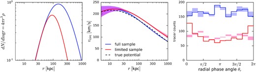
Illustration of the potential bias caused by incomplete tracer sample (see text for details).