


ABSTRACT
We report on the masses (MWD), effective temperatures (|$\rm{T_\mathrm{eff}}$|), and secular mean accretion rates (|$\langle \dot{M} \rangle$|) of 43 cataclysmic variable (CV) white dwarfs, 42 of which were obtained from the combined analysis of their Hubble Space Telescope ultraviolet data with the parallaxes provided by the Early Third Data Release of the Gaia space mission, and one from the white dwarf gravitational redshift. Our results double the number of CV white dwarfs with an accurate mass measurement, bringing the total census to 89 systems. From the study of the mass distribution, we derive |$\langle M_\mathrm{WD} \rangle = 0.81^{+0.16}_{-0.20}\, \mathrm{M_\odot }$|, in perfect agreement with previous results, and find no evidence of any evolution of the mass with orbital period. Moreover, we identify five systems with MWD < 0.5 M⊙, which are most likely representative of helium-core white dwarfs, showing that these CVs are present in the overall population. We reveal the presence of an anticorrelation between the average accretion rates and the white dwarf masses for the systems below the |$2\!-\!3\,$| h period gap. Since |$\langle \dot{M} \rangle$| reflects the rate of system angular momentum loss, this correlation suggests the presence of an additional mechanism of angular momentum loss that is more efficient at low white dwarf masses. This is the fundamental concept of the recently proposed empirical prescription of consequential angular momentum loss (eCAML) and our results provide observational support for it, although we also highlight how its current recipe needs to be refined to better reproduce the observed scatter in |$\rm{T_\mathrm{eff}}$| and |$\langle \dot{M} \rangle$|, and the presence of helium-core white dwarfs.
1 INTRODUCTION
Cataclysmic variables (CVs) are compact interacting binaries in which a white dwarf is accreting mass from a low-mass star via Roche lobe overflow (e.g. Warner 1995). CVs descend from main-sequence binaries in which the more massive star (the primary) evolves first and leaves the main sequence. Following its expansion, the primary star fills its Roche lobe and starts unstable mass transfer on its less massive companion (the secondary), leading to the formation of a common envelope, i.e. a shared photosphere engulfing both stars (e.g. Paczynski 1976; Ivanova et al. 2013). The two stars transfer orbital energy to the envelope, which is rapidly expelled, leaving behind a post-common envelope binary composed of the core of the giant primary, which evolves into a white dwarf, and a low-mass secondary star. Owing to subsequent orbital angular momentum losses, mainly via magnetic braking (which arises from a stellar wind associated with the magnetic activity of the secondary, e.g. Mestel 1968; Verbunt & Zwaan 1981) and gravitational wave radiation (e.g. Paczyński 1967), the post-common envelope binary evolves into a semi-detached configuration, becoming a CV.
During the CV phase, the white dwarf response to the mass accretion process is the subject of a long-standing debate. Many binary population studies predict an average mass of CV white dwarfs of |$\langle M_\mathrm{WD} \rangle \simeq 0.5\, \mathrm{M_\odot }$| (e.g. de Kool 1992; Politano 1996), which is lower than that of single white dwarfs (|$\langle M_\mathrm{WD} \rangle \simeq 0.6\, \mathrm{M_\odot }$|, Koester, Schulz & Weidemann 1979; Liebert et al. 2005; Kepler et al. 2007). This is because it is expected that the core growth of the primary is halted by the onset of the common envelope phase. Moreover, once a CV is formed, the material piled up at the white dwarf surface is compressed by the strong gravitational field of the star, leading periodically (typically on time-scale of ten/hundred thousands of years) to the occurrence of classical nova eruptions. These are the result of the thermonuclear ignition of the accreted material on the white dwarf surface and, during these explosions, different theoretical models predict that the accreted material (e.g. Yaron et al. 2005) and part of the underlying core of the white dwarf (Gehrz et al. 1998; Epelstain et al. 2007) should be ejected in the surrounding space, thus preventing the white dwarf from growing in mass. However, white dwarfs in CVs have been found to be significantly more massive than binary population models predicted (e.g. de Kool 1992; Politano 1996), with early work showing the average mass of CV white dwarfs to lie in the range |$\langle M_\mathrm{WD} \rangle \simeq 0.8\!-\!1.2\, \mathrm{M}_\odot$| (Warner 1973; Ritter 1987). This result was originally interpreted as an observational bias because (i) the higher the mass of the white dwarf, the larger the accretion energy released per accreted unit mass, and (ii) for a fixed donor mass, more massive white dwarfs have larger Roche lobes that can accommodate larger, and hence brighter (especially at optically wavelengths) accretion discs. Therefore, CVs hosting massive white dwarfs were expected to be more easily discovered in magnitude limited samples (Ritter & Burkert 1986). Later on, Zorotovic, Schreiber & Gänsicke (2011) reviewed the masses of CV white dwarfs available in the literature, showing that the average mass of CV white dwarfs is |$\langle M_\mathrm{WD} \rangle = 0.83 \pm 0.23\, \mathrm{M}_\odot$|. Using the large and homogeneous sample of systems (Szkody et al. 2011, and references therein) discovered by the Sloan Digital Sky Survey (SDSS; York et al. 2000), the authors also demonstrated that there is a clear trend in disfavouring the detection of massive white dwarfs (which are smaller and less luminous than low-mass white dwarfs for the same |$\rm{T_\mathrm{eff}}$|) and therefore the high average mass of CV white dwarfs cannot be ascribed to an observational bias.
Following this result, several authors investigated the possibility that CV white dwarfs could efficiently retain the accreted material and grow in mass, either by ejecting less material than they accrete, via quasi-steady helium burning after several nova cycles (Hillman et al. 2016), or through a phase of thermal time-scale mass transfer during the pre-CV phase (Schenker et al. 2002). Wijnen, Zorotovic & Schreiber (2015) argued that mass growth during nova cycles cannot reproduce the observed distribution. In addition, these authors found that, even though the white dwarf mass could increase during thermal time-scale mass transfer, the resulting CV population would harbour a much higher fraction of nuclear evolved donor stars than observed, and thus they concluded that mass growth does not seem to be the reason behind the high masses of CV white dwarfs. A general consensus on the ability of the white dwarf to retain the accreted mass has not been reached yet (Hillman et al. 2020; Starrfield et al. 2020). Moreover, neither mechanism is able to explain the observed CV white dwarf mass distribution without creating conflicts with other observational constraints.
A promising alternative solution proposed throughout the last couple of years assumes that the standard CV evolution model is incomplete. Schreiber, Zorotovic & Wijnen (2016) suggested that consequential angular momentum loss (CAML) is the key missing ingredient. This sort of angular momentum loss arises from the mass transfer process itself and acts in addition to magnetic braking and gravitational wave radiation. Schreiber et al. (2016) developed an empirical model (eCAML) in which the strength of CAML is inversely proportional to the white dwarf mass, leading to dynamically unstable mass transfer in most CVs hosting low-mass white dwarfs (|$M_\mathrm{WD} \lesssim 0.6\, \mathrm{M_\odot }$|). The majority of these systems would not survive as semi-detached binaries but the two stellar components would instead merge into a single object (see also Nelemans et al. 2016). The main strength of the eCAML model is that it can also solve other disagreements between theory and observations, such as the observed CV space density and orbital period distribution (Zorotovic & Schreiber 2017; Belloni et al. 2018, 2020; Pala et al. 2020), without the requirement of additional fine tuning. However, the exact physical mechanism behind this additional source of angular momentum loss and the reason for its dependence on the white dwarf mass are still unclear.
Finally, it has to be considered that, while observational biases can be ruled out, it is more difficult to assess the presence of systematics affecting Zorotovic et al. (2011)’s results, which were based on a sample of only 32 systems with accurate mass measurements, 22 of which were derived from the analysis of their eclipse light curves. Given that the previous results were mainly based on one methodology, it is necessary to increase the number of systems with an accurate mass measurement and diversify the methods employed in order to confirm the inferred high masses of CV white dwarfs, which remains one of the biggest and unresolved issues for the theoretical modelling of CV evolution.
An alternative method to measure CV white dwarf masses consists of the analysis of their ultraviolet spectra. The ultraviolet waveband is optimal for studying the underlying white dwarfs as they are relatively hot (|$\rm{T_\mathrm{eff}} \gtrsim 10\, 000\,$| K, Sion 1999; Pala et al. 2017) and dominate the emission at these wavelengths, while the optical waveband is contaminated by the emission from the accretion flow and the companion star. From the knowledge of the distance to the system, the white dwarf radius (RWD) can be derived from the scaling factor between the best-fitting model and the ultraviolet spectrum. Under the assumption of a mass–radius relationship, it is then possible to measure the white dwarf mass. Another possibility is to perform a dynamical study. The radial velocities of the white dwarf and the donor allow to infer the white dwarf gravitational redshift that, combined with a mass-radius relationship, provides the mass of the white dwarf.
Over the last 30 years, the Hubble Space Telescope (HST) has proven to be essential for the study of CVs, delivering ultraviolet observations1 for 193 systems. Nonetheless, in the past, only a handful of objects had mass measurements derived from the analysis of their ultraviolet data because of the lack of accurate CV distances. In this respect, the Gaia space mission represents a milestone for CV research, delivering accurate parallaxes for a large number of these interacting binaries, finally enabling a quantitative analysis of the ultraviolet data obtained over the past decades.
We here analyse the HST observations of 43 CVs for which the white dwarf is the dominant source of emission in the ultraviolet wavelength range, and for which Gaia parallaxes from the Third Early Data release (EDR3) are available. To provide an additional independent determination to test our results and assess the presence of systematics, we complement this data set with optical phase-resolved observations obtained with X-shooter mounted on the Very Large Telescope (VLT), which provides independent dynamical mass measurements. We present this large CV sample, which doubles the number of objects with accurate MWD measurements, providing new constraints on the response of the white dwarf to the mass accretion process, and for the further development of models for CV evolution.
2 SAMPLE SELECTION AND OBSERVATIONS
2.1 Ultraviolet observations
Among the 193 systems in the HST ultraviolet archive, 191 have a Gaia EDR3 parallax (Table 45 of the online material) and have been observed with either the Goddard High Resolution Spectrograph (GHRS), the Faint Object Spectrograph (FOS), the Space Telescope Imaging Spectrograph (STIS), or the Cosmic Origin Spectrograph (COS) with a setup suitable for our analysis, i.e. (at least) the full coverage of the Ly α (|$1100\!-\!1600\,$| Å) from the white dwarf photosphere with a resolution of R ≃ 1000–3000. Together with a signal-to-noise ratio (SNR) of at least ≃10 and the knowledge of the distance to the systems, this setup allows an accurate determination of the white dwarf effective temperatures, chemical abundances, and masses (Gänsicke et al. 2005).
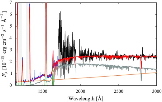
CVs are characterized by an intrinsic variable behaviour that can affect the analysis of their ultraviolet data. A large fraction of CVs spend most of their time in a quiescent state, in which the accretion rate on to the white dwarf is very low, though the mass buffered in the accretion disc is slowly built up. During this phase, the white dwarf dominates the spectral appearance of the system and, at ultraviolet wavelengths, is recognisable from broad Ly α absorption centred on |$1216\,$| Å. The profile of Ly α changes with Teff, becoming more defined and narrower in the hotter white dwarfs, while the continuum slope of the spectrum becomes steeper (Fig. 1). Periods of quiescence are interrupted by sudden brightenings with amplitudes of 2–5 mag and, occasionally up to 9 mag (Maza & Gonzalez 1983; Warner 1995; Templeton 2007), called dwarf nova outbursts, when a fraction of the disc mass is rapidly drained on to the white dwarf. These outbursts arise from thermal-viscous instabilities in their accretion discs, causing a variation in the mass transfer rate through them (Osaki 1974; Meyer & Meyer-Hofmeister 1984; Hameury et al. 1998). Immediately after the occurrence of an outburst, the disc is hot and while it cools down it can partially or totally outshine the emission of the white dwarf even in the ultraviolet (top panel of Fig. 2).
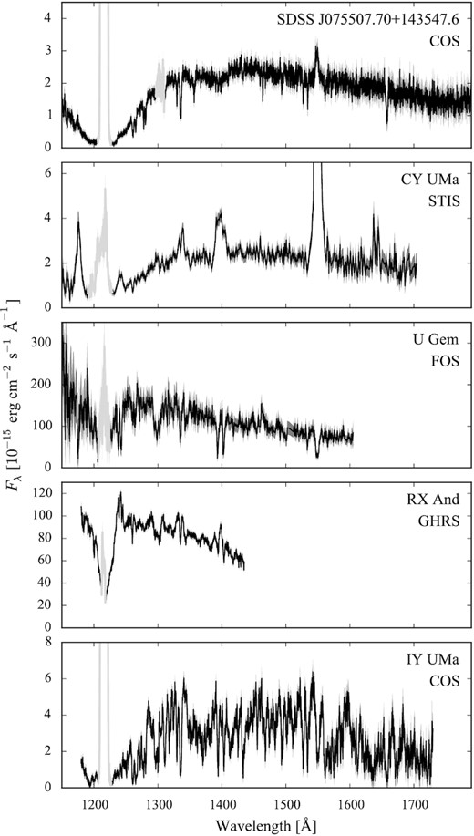
Sample HST spectra showing, from top to bottom, four typical quiescent CVs (SDSS J075507.70+143547.6, CY UMa, U Gem, and RX And) observed with different HST instruments, and one eclipsing system (IY UMa) whose spectrum is characterized by the presence of the iron-curtain. The geocoronal emission lines of Ly α (|$1216\,$| Å) and O i (|$1302\,$| Å, not always detected) are plotted in grey.
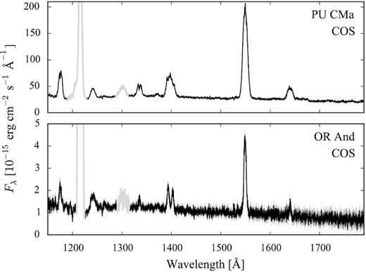
Sample HST spectra of a dwarf nova observed four days after a disc outburst (PU CMa, top panel) and a nova-like star observed in its normal high state (OR And, bottom panel). The spectra are dominated by the disc emission rather than the white dwarf. The geocoronal emission lines of Ly α (|$1216\,$| Å) and O i (|$1302\,$| Å) are plotted in grey.
Following an outburst, the white dwarf is heated as a consequence of the increased infall of material, and this can possibly give rise to a non-homogeneous distribution of the temperature across its visible surface. Heated accretion belts or hot spots can dominate the overall ultraviolet emission of the system and the resulting temperature gradient results in the white dwarf radius being underestimated (e.g Toloza et al. 2016; Pala et al. 2019). The presence of a hot spot can be easily unveiled thanks to the modulation it introduces in the light curve of the system. In contrast, an equatorial accretion belt (Kippenhahn & Thomas 1978) can be difficult to detect since, being symmetric with respect to the rotation axis of the white dwarf, it does not cause variability on the white dwarf spin period (e.g GW Lib; Toloza et al. 2016). Therefore, the analysis of the ultraviolet data obtained after a disc outburst provides only an upper limit on the white dwarf effective temperature and radius and, in turn, only a lower limit on its mass.
Additionally, members of a sub-class of CVs, known as nova-like systems, are characterized by high mean mass-transfer rates which usually keep the discs in a stable hot state, equivalent to a dwarf nova in permanent outburst. In this high state, the disc dominates the spectral appearance even in the far-ultraviolet, preventing a direct detection of the white dwarf (bottom panel of Fig. 2). However, occasionally, it is thought that as a consequence of starspots appearing in, or migrating into the tip of the donor star at the first Lagrangian point (Livio & Pringle 1994), the mass transfer rate drops (low state) and unveils the white dwarf (e.g. Gänsicke & Koester 1999; Knigge et al. 2000; Hoard et al. 2004). These low states typically last for days up to years (e.g Rodríguez-Gil et al. 2007) and provide a window in which the white dwarf parameters can be measured (e.g. Gänsicke et al. 1999; Knigge et al. 2000; Hoard et al. 2004).
While some nova-likes can be magnetic, similar behaviour is observed in highly magnetic CVs. A significant number (28 per cent, Pala et al. 2020) of CVs contain strongly (|$B \gtrsim 10\, \mathrm{MG}$|) magnetic white dwarfs, whose magnetism suppresses the formation of an accretion disc and forces the accretion flow to follow the field lines. The strong field of the white dwarf may have a deep impact on the evolution of the system (Schreiber et al. 2021). Similar to nova-likes, magnetic CVs are also characterized by alternating between high and low states, on time-scales of months to years. During high states, mass accretion is stable and the ultraviolet emission is dominated by a hot polar cap close to one (or both) the magnetic pole(s) of the white dwarf. During low states, the hot-caps emission is greatly weakened and the white dwarf dominates the spectral appearance of the system. Possibly, low states in magnetic CVs are also triggered by a donor stellar spot passing around the first Lagrangian point region (Hessman, Gänsicke & Mattei 2000). In low states, time-resolved observations are required in order to account for the possible contribution from the accretion cap and to obtain accurate white dwarf parameters.
Finally, CVs experience (at least once in their life) powerful classical nova eruptions due to thermonuclear runaways at their surface. CVs that have been observed to undergo these eruptions are known as novae and their ultraviolet spectra are dominated by the emission from a hot highly variable component (e.g. Cassatella, Altamore & González-Riestra 2005), whose origin is still not clear, that prevents the direct detection of the white dwarf.
To account for the high variable nature of CVs, we inspected the archival ultraviolet HST data and discarded (i) dwarf novae observed during or immediately after a disc outburst; (ii) nova-likes in high state and novae and (iii) polars lacking time-resolved observations with sufficient orbital phase coverage, necessary to determine a spectrum of the underlying white dwarf (see e.g. Gänsicke et al. 2006). In addition, we also discarded systems hosting a nuclear evolved donor. These CVs descend from binaries that underwent a thermal-time-scale mass transfer phase (Schenker et al. 2002) and can be easily identified from their enhanced N v/C iv line flux ratios (Gänsicke et al. 2003). In these systems, the white dwarf accretes helium rich material from its companion and this anomalously large helium abundance can cause an asymmetrical broadening of the blue wing of the Ly α (Gänsicke et al. 2018), thus affecting the estimates of the white dwarf surface gravity and temperature (Toloza et al., in preparation).
The final sample consists of 43 systems2 and a log of their spectroscopic observations is presented in Table 1, while the different observational setups are listed in Table 2. Finally, the full list of CVs observed with HST is provided in Section 5 of the online material.
Log of the HST ultraviolet observations of the 43 CV white dwarfs studied in this work along with the corresponding Gaia EDR3 parallaxes (corrected for the zero-point, see Section 2.1.1), sorted by increasing orbital period. The distances have been computed following the method described in Pala et al. (2020), assuming the reported scale height h. The colour excess E(B − V) have been derived using the STructuring by Inversion the Local Interstellar Medium (Stilism) reddening map (Lallement et al. 2018). Systems highlighted with a star symbol are known to be eclipsing.
| System | Porb | h | E(B − V) | Instrument | Grating | Central | Total | Observation | Gaia EDR3 ID | ϖ | d |
|---|---|---|---|---|---|---|---|---|---|---|---|
| (min) | (pc) | (mag) | λ | exposure | date | (mas) | (pc) | ||||
| (Å) | time (s) | ||||||||||
| SDSS J150722.30 + 523039.8* | 66.61 | 260 | |$0.018^{+0.006}_{-0.018}$| | COS | G140L | 1230 | 9762 | 2010 Feb 18 | 1593140224924964864 | 4.73 ± 0.09 | 211 ± 4 |
| STIS | G230LB | 2375 | 5226 | ||||||||
| SDSS J074531.91 + 453829.5 | 76.0 | 260 | 0.027 ± 0.017 | COS | G140L | 1105 | 5486 | 2012 Mar 13 | 927255749553754880 | 3.2 ± 0.2 | |$310^{+23}_{-20}$| |
| GW Lib | 76.78 | 260 | 0.022 ± 0.018 | COS | G140L | 1105 | 7417 | 2013 May 30 | 6226943645600487552 | 8.88 ± 0.06 | 112.6 ± 0.8 |
| SDSS J143544.02 + 233638.7 | 78.0 | 260 | 0.02 ± 0.02 | COS | G140L | 1105 | 7123 | 2013 Mar 09 | 1242828982729309952 | 4.8 ± 0.2 | |$208^{+9}_{-8}$| |
| OT J213806.6 + 261957 | 78.1 | 260 | 0.017 ± 0.015 | COS | G140L | 1105 | 4760 | 2013 Jul 25 | 1800384942558699008 | 10.11 ± 0.04 | 98.9 ± 0.4 |
| BW Scl | 78.23 | 260 | |$0.002^{+0.015}_{-0.002}$| | STIS | E140M | 1425 | 1977 | 2006 Dec 27 | 2307289214897332480 | 10.71 ± 0.05 | 93.4 ± 0.5 |
| LL And | 79.28 | 260 | |$0.06^{+0}_{-0.02}$| | STIS | G140L | 1425 | 4499 | 2000 Dec 07 | 2809168096329043712 | 1.6 ± 0.6 | |$609^{+343}_{-205}$| |
| AL Com | 81.6 | 260 | 0.045 ± 0.018 | STIS | G140L | 1425 | 4380 | 2000 Nov 27 | 3932951035266314496 | 1.9 ± 0.6 | |$523^{+252}_{-149}$| |
| WZ Sge | 81.63 | 260 | |$0.003^{+0.015}_{-0.003}$| | FOS | G130H | 1600 | 3000 | 1992 Oct 08 | 1809844934461976832 | 22.14 ± 0.03 | 45.17 ± 0.06 |
| SW UMa | 81.81 | 260 | |$0.008^{+0.017}_{-0.008}$| | STIS | G140L | 1425 | 4933 | 2000 Mar 26 | 1030279027003254784 | 6.23 ± 0.06 | 160.6 ± 1.6 |
| V1108 Her | 81.87 | 260 | 0.046 ± 0.019 | COS | G140L | 1105 | 7327 | 2013 Jun 06 | 4538504384210935424 | 6.8 ± 0.1 | 148 ± 2 |
| ASAS J002511 + 1217.2 | 82.0 | 260 | |$0.009^{+0.016}_{-0.009}$| | COS | G140L | 1105 | 7183 | 2012 Nov 15 | 2754909740118313344 | 6.4 ± 0.1 | 157 ± 3 |
| HV Vir | 82.18 | 260 | |$0.024^{+0.012}_{-0.021}$| | STIS | G140L | 1425 | 4535 | 2000 Jun 10 | 3688359000015020800 | 3.2 ± 0.3 | |$317^{+29}_{-25}$| |
| SDSS J103533.02 + 055158.4* | 82.22 | 260 | |$0.017^{+0.018}_{-0.017}$| | COS | G140L | 1105 | 12282 | 2013 Mar 08 | 3859020040917830400 | 5.1 ± 0.3 | |$195^{+12}_{-10}$| |
| WX Cet | 83.90 | 260 | |$0.013^{+0.016}_{-0.013}$| | STIS | E140M | 1425 | 7299 | 2000 Oct 30 | 2355217815809560192 | 3.97 ± 0.13 | |$252^{+9}_{-8}$| |
| SDSS J075507.70 + 143547.6 | 84.76 | 260 | |$0.011^{+0.015}_{-0.011}$| | COS | G140L | 1105 | 7183 | 2012 Dec 14 | 654539826068054400 | 4.2 ± 0.2 | |$239^{+12}_{-11}$| |
| SDSS J080434.20 + 510349.2 | 84.97 | 260 | |$0.007^{+0.016}_{-0.007}$| | COS | G140L | 1105 | 5415 | 2011 Nov 03 | 935056333580267392 | 7.03 ± 0.11 | 142 ± 2 |
| EG Cnc | 86.36 | 260 | |$0.008^{+0.017}_{-0.008}$| | STIS | G140L | 1425 | 4579 | 2006 Dec 20 | 703580960947960576 | 5.4 ± 0.2 | 186 ± 7 |
| EK TrA | 86.36 | 260 | 0.034 ± 0.019 | STIS | E140M | 1425 | 4302 | 1999 Jul 25 | 5825198967486003072 | 6.61 ± 0.04 | 151.4 ± 0.8 |
| 1RXS J105010.8–140431 | 88.56 | 450 | |$0.005^{+0.015}_{-0.005}$| | COS | G140L | 1105 | 7363 | 2013 May 10 | 3750072904055666176 | 9.19 ± 0.09 | 109 ± 1 |
| BC UMa | 90.16 | 260 | |$0.017^{+0}_{-0.017}$| | STIS | G140L | 1425 | 12998 | 2000 Jul 18 | 787683052032971904 | 3.41 ± 0.13 | |$293^{+11}_{-10}$| |
| VY Aqr | 90.85 | 260 | |$0.008^{+0.016}_{-0.008}$| | STIS | E140M | 1425 | 7250 | 2000 Jul 10 | 6896767366186700416 | 7.08 ± 0.09 | |$141.3^{+1.9}_{-1.8}$| |
| QZ Lib | 92.36 | 450 | 0.10 ± 0.03 | COS | G140L | 1105 | 7512 | 2013 Apr 26 | 6318149711371454464 | 5.0 ± 0.2 | |$199^{+11}_{-10}$| |
| SDSS J153817.35 + 512338.0 | 93.11 | 260 | 0.027 ± 0.018 | COS | G140L | 1105 | 4704 | 2013 May 16 | 1595085299649674240 | 1.64 ± 0.12 | |$607^{+47}_{-40}$| |
| UV Per | 93.44 | 260 | 0.07 ± 0.04 | STIS | G140L | 1425 | 900 | 2002 Oct 11 | 457106501671769472 | 4.04 ± 0.11 | |$248^{+7}_{-6}$| |
| 1RXS J023238.8–371812 | 95.04 | 450 | |$0.005^{+0.014}_{-0.005}$| | COS | G140L | 1105 | 12556 | 2012 Nov 01 | 4953766320874344704 | 4.68 ± 0.16 | |$214^{+8}_{-7}$| |
| RZ Sge | 98.32 | 260 | 0.03 ± 0.3 | STIS | G140L | 1425 | 900 | 2003 Jun 13 | 1820209309025797888 | 3.40 ± 0.08 | 294 ± 7 |
| CY UMa | 100.18 | 260 | |$0.018^{+0}_{-0.015}$| | STIS | G140L | 1425 | 830 | 2002 Dec 27 | 832942871937909632 | 3.27 ± 0.07 | 306 ± 6 |
| GD 552 | 102.73 | 450 | |$0.007^{+0.015}_{-0.007}$| | STIS | G140L | 1425 | 14580 | 2002 Oct 24 | 2208124536065383424 | 12.41 ± 0.04 | 80.6 ± 0.2 |
| G230LB | 2375 | 4230 | 2002 Aug 31 | ||||||||
| IY UMa* | 106.43 | 260 | |$0.015^{+0}_{-0.015}$| | COS | G140L | 1105 | 4195 | 2013 Mar 30 | 855167540988615296 | 5.52 ± 0.07 | 181 ± 2 |
| SDSS J100515.38 + 191107.9 | 107.6 | 260 | |$0.021^{+0.011}_{-0.014}$| | COS | G140L | 1105 | 7093 | 2013 Jan 31 | 626719772406892288 | 2.95 ± 0.17 | |$339^{+21}_{-19}$| |
| RZ Leo | 110.17 | 260 | |$0.023^{+0.015}_{-0.023}$| | COS | G140L | 1105 | 10505 | 2013 Apr 11 | 3799290858445023488 | 3.59 ± 0.15 | |$279^{+12}_{-11}$| |
| AX For | 113.04 | 260 | 0.018 ± 0.018 | COS | G140L | 1105 | 7483 | 2013 Jul 11 | 5067753236787919232 | 2.86 ± 0.08 | 349 ± 10 |
| CU Vel | 113.04 | 260 | |$0.007^{+0.015}_{-0.007}$| | COS | G140L | 1105 | 4634 | 2013 Jan 18 | 5524430207364715520 | 6.31 ± 0.04 | 158 ± 1 |
| EF Peg | 120.53 | 120 | 0.048 ± 0.019 | STIS | E140M | 1425 | 6883 | 2000 Jun 18 | 1759321791033449472 | 3.5 ± 0.2 | |$288^{+21}_{-18}$| |
| DV UMa* | 123.62 | 120 | |$0.02^{+0}_{-0.012}$| | STIS | G140L | 1425 | 900 | 2004 Feb 08 | 820959638305816448 | 2.60 ± 0.15 | |$382^{+24}_{-21}$| |
| IR Com* | 125.34 | 120 | |$0.019^{+0.021}_{-0.019}$| | COS | G140L | 1105 | 6866 | 2013 Jul 11 | 3955313418148878080 | 4.63 ± 0.06 | 216 ± 3 |
| AM Her | 185.65 | 120 | 0.017 ± 0.016 | STIS | G140L | 1425 | 10980 | 2002 Jul 11/12 | 2123837555230207744 | 11.37 ± 0.03 | 87.9 ± 0.2 |
| DW UMa* | 196.71 | 120 | |$0.009^{+0.018}_{-0.009}$| | STIS | G140L | 1425 | 26144 | 1999 Jan 25 | 855119196836523008 | 1.73 ± 0.02 | |$579^{+7}_{-6}$| |
| U Gem | 254.74 | 120 | |$0.003^{+0.015}_{-0.003}$| | FOS | G130H | 1600 | 360 | 1992 Sep 28 | 674214551557961984 | 10.75 ± 0.03 | 93.0 ± 0.3 |
| SS Aur | 263.23 | 120 | 0.047 ± 0.033 | STIS | G140L | 1425 | 600 | 2003 Mar 20 | 968824328534823936 | 4.02 ± 0.03 | 249 ± 2 |
| RX And | 302.25 | 120 | 0.02 ± 0.02 | GHRS | G140L | 1425 | 1425 | 1996 Dec 22 | 374510294830244992 | 5.08 ± 0.03 | 197 ± 1 |
| V442 Cen | 662.4 | 120 | 0.048 ± 0.015 | STIS | G140L | 1425 | 700 | 2002 Dec 29 | 5398867830598349952 | 2.92 ± 0.04 | 343 ± 5 |
Notes. For several systems in our sample, IUE spectroscopic observations covering the wavelength range 1800–3200 Å are available. These data allow to estimate the interstellar reddening due to dust absorption from the bump at |$\simeq 2175\,$| Å and their analysis is available in the literature (CU Vel, Pala et al. 2017; DW UMa, Szkody 1987; AM Her, Raymond et al. 1979; UV Per, Szkody 1985; SW UMa, WZ Sge, U Gem, RX And, VY Aqr and SS Aur, La Dous 1991). The E(B − V) literature measurements from IUE are all in agreement with those from Stilism. However, since the former do not have associated uncertainties, we decided to adopt the latter in our analysis, since Stilism provides the corresponding uncertainties and allows us to properly account for them when evaluating those associate with the white dwarf parameters.
Characteristics of the gratings and setup of the HST observations used in this work.
| Instrument | Aperture | Grating | Central | Wavelength | Resolution |
|---|---|---|---|---|---|
| wavelengthe | coverage | ||||
| COS | PSAa | G140L | 1105 Å | |$1105\!-\!1730$| Å | ≃3000 |
| FOS | 1″ | G130H | 1600 Å | |$1150\!-\!1610$| Å | ≃1200 |
| GHRS | LSAb | G140L | 1425 Å | |$1149\!-\!1435\,$| Å | ≃2000 |
| STIS | 0.2″ × 0.2″ | E140Mc | 1425 Å | |$1125\!-\!1710\,$| Å | ≃|$90\, 000$| |
| 52″ × 0.2″ | G140L | 1425 Å | |$1150\!-\!1700\,$| Å | ≃1000 | |
| G230Ld | 2375 Å | |$1650\!-\!3150\,$| Å | ≃800 |
Primary Science Aperture (2.5″).
Large Science Aperture (2.0″).
We re-bin the data obtained with the E140M grating to match the resolution of the G140L observations in order to increase the signal-to-noise ratio.
Only used in the cases of SDSS J150722.30+523039.8 and GD 552 to complement the G140L data, which provide the full coverage of Ly α from the white dwarf photosphere.
The central wavelength is defined as the shortest wavelength recorded on the Segment A of the detector.
2.1.1 Quality of the Gaia data
Gaia astrometric solutions, and thereby parallaxes, are known to be affected by systematics arising from imperfections in the instrument and data processing methods (Lindegren et al. 2020). The mean value of the systematic error, the so-called parallax zero-point ϖzp, can be modelled according to the ecliptic latitude, magnitude, and colour of each Gaia EDR3 source. We employed the python code provided by the Gaia consortium3 to compute ϖzp for our targets, and corrected their parallaxes by subtracting the estimated zero-point to the quoted Gaia EDR3 parallaxes. This correction ranges from 0.5 |$\mu$|as, in the case of V1108 Her, to −43 |$\mu$|as for U Gem.
Together with the main kinematic parameters (positions, proper motions, and magnitudes), which are used to derive the astrometric solution for each source, Gaia EDR3 also provides a series of ancillary parameters that can be used to evaluate the accuracy of this solution. Among the most relevant ones is the astrometric_excess_noise, which represents the error associated with the astrometric modelling (see Lindegren et al. 2012) and that, ideally, should be zero. Following Pala et al. (2020), we verified that the sources in our sample have reliable parallaxes by satisfying the condition astrometric_excess_noise < 2.
Converting parallaxes into distances is not always trivial as the mere inversion of the parallax can introduce some biases in the distance estimate, especially when the fractional error on the parallax is larger than 20 per cent (see e.g. Bailer-Jones 2015; Luri et al. 2018), which is the case for two systems in our sample, AL Com and LL And. Their large uncertainties are most likely related to their intrinsic faintness (G = 19.7, G = 20.1, respectively) since the other Gaia parameters that flag possible issues with the astronometric solution (astrometric_excess_noise and RUWE, described below) are within the range expected for well-behaved sources. We therefore computed the distance to each CV using a statistical approach, in which we assumed an exponentially decreasing volume density prior and a scale height h following the method4 described in Pala et al. (2020). Typically, the distances computed with the two methods differ by less than one per cent, the only exception being LL And with a difference of five per cent (Fig. 3).
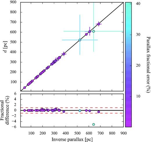
Comparison between the distances to our targets computed as the inverse of the parallax (ϖ−1) and using a statistical approach via the assumption of an exponentially decreasing volume density prior. The data are colour coded according to the parallax fractional error. The fractional difference, defined as (D − ϖ−1)/ϖ−1, between the two methods is typically less than one per cent (red dashed lines in the bottom panel).
Another important parameter to assess the reliability of the parallaxes is the normalized unit weight error (RUWE). This represents the square root of the normalized chi-square of the astrometric fit, scaled according to the source magnitude G, its effective wavenumber |$\nu_\mathrm{eff}$| and its pseudocolour |$\hat{\nu }_\mathrm{eff}$| (see Lindegren et al. 2020 for more details). Ideally, for well-behaved sources,5RUWE < 1.4. However, we noticed that for the system in our sample with the largest RUWE, AM Her (RUWE = 2.8), the distance derived from its Gaia parallax (|$88.1 \pm 0.4\,$| pc) is consistent with the distance estimated by Thorstensen (2003), |$79^{+9}_{-6}\,$|pc. Similarly, in the case of U Gem, another system with high weight error (RUWE = 2.4), its Gaia parallax (ϖ = 10.75 ± 0.03 mas) and corresponding distance (|$93.4 \pm 0.5\,$| pc) are in good agreement, respectively, with the parallax measurements obtained using the HST Fine Guidance Sensors by Harrison et al. (2000) (ϖ = 10.30 ± 0.50 mas) and Harrison et al. (2004) (ϖ = 9.96 ± 0.37 mas), and with the distance estimated by Beuermann (2006), |$97\pm \, 7$|pc. These large values of RUWE are most likely related to colour variations of the systems during different Gaia observations, caused either by the occurrence of low and high states in AM Her (Gänsicke et al. 2006), and disc outbursts in U Gem. Nonetheless, since their Gaia astrometry still provides reliable distances, we decided to not apply any cut on this parameter for the remaining systems, which all have lower RUWE values.
2.2 Optical spectroscopy
We obtained complementary phase-resolved spectroscopy with X-shooter (Vernet et al. 2011) of the 22 targets from the HST sample that are visible from the Southern hemisphere and in which (i) the white dwarf dominates the of emission in the ultraviolet and (ii) for which no dynamical study has been carried out before.
X-shooter is an échelle spectrograph located at the Cassegrain focus of UT2 of the VLT at the European Southern Observatory (ESO) in Cerro Paranal (Chile). It is equipped with three arms: blue (UVB, |$\lambda \simeq 3000\!-\!5595\,$| Å), visual (VIS, |$\lambda \simeq 5595\!-\!10\, 240\,$| Å), and near-infrared (NIR, |$\lambda \simeq 10\, 240\!-\!24\, 800\,$| Å), with a medium spectral resolution (|$R \simeq 5000\!-\!10\, 000$|). For each arm, the slit width was chosen to best match the seeing and the exposure times were set with the aim to optimize the SNR and, at the same time, to minimize the orbital smearing. At the time of the observations the atmospheric dispersion correctors of X-shooter were broken and hence the slit angle was reset to the parallactic angle position after one hour of exposures. The data were reduced using the Reflex pipeline (Freudling et al. 2013). To account for the well-documented wavelength shift between the three arms,6 we used theoretical templates of sky emission lines to calculate the shift of each spectrum with respect to the expected position. We then applied this shift together with the barycentric radial velocity correction to the data. Finally, a telluric correction was performed using molecfit (Kausch et al. 2015; Smette et al. 2015).
In the spectra of three (AX For, IR Com, and V1108 Her) of the 22 CVs observed with X-shooter, we identified the Mg ii absorption line at 4481 Å that originates in the white dwarf photosphere, and several absorption features arising from the secondary photosphere, including Na i (|$11\, 381/11\, 403$| Å), K i (|$11\, 690/11\, 769$| and |$12\, 432/12\, 522$| Å). The K i and Mg ii lines, were used to track the motion of the two stellar components and to reconstruct their radial velocity curves from which the mass of the white dwarf can be determined. A log of the spectroscopic observations is presented in Table 3.
Log of the optical observations of the three CVs observed with X-shooter in which the signatures of both the white dwarf and the secondary star were identified in their spectra. We obtained time-series of N spectra with T exposure time each.
| UVB | VIS | NIR | ||||||||
|---|---|---|---|---|---|---|---|---|---|---|
| Observation | Exposure | Slit | Resolution | Exposure | Slit | Resolution | Exposure | Slit | Resolution | |
| date | time | width | time | width | time | width | ||||
| System | (YYYY-MM-DD) | N × T(s) | (arcsec) | (Å) | N × T (s) | (arcsec) | (Å) | N × T (s) | (arcsec) | (Å) |
| AX For | 2013-10-25 | 7 × 606 | 1.0 | 0.99 | 13 × 294 | 0.9 | 0.90 | 22 × 200 | 0.9 | 2.11 |
| 2015-09-24 | 12 × 610 | 1.3 | 1.10 | 12 × 592 | 1.2 | 0.90 | 12 × 642 | 1.2 | 2.06 | |
| IR Com | 2014-03-05 | 29 × 270 | 1.0 | 1.01 | 21 × 412 | 0.9 | 0.89 | 31 × 300 | 0.9 | 2.02 |
| V1108 Her | 2015-05-12 | 12 × 480 | 1.0 | 1.04 | 10 × 587 | 0.9 | 0.92 | 12 × 520 | 0.9 | 2.07 |
In the remaining 19 systems, we identified only signatures of either the white dwarf or the secondary, and in some cases of neither of them, and the analysis of these objects will be presented elsewhere.
3 METHODS
3.1 Light curve analysis
Throughout the duration of the individual HST observations (typically a few hours), CVs can show different types of variability, such as eclipses, modulations due to the white dwarf rotation, white dwarf pulsations, double humps, and brightenings (e.g. Szkody et al. 2002b; Araujo-Betancor et al. 2003; Toloza et al. 2016; Szkody et al. 2017; Pala et al. 2019). Eclipses are particularly important since they allow a white dwarf mass measurement based only on geometrical assumptions to be obtained. In contrast, pulsations and brightenings reflect the presence of hot spots and, more generally, of a gradient in temperature over the visible white dwarf surface. When in view, the emission of the hot spots can dominate the overall ultraviolet emission of the system making the white dwarf look hotter and affecting both the temperature and mass estimates (Toloza et al. 2016; Pala et al. 2019). Therefore, it is important to remove the contribution of these spurious sources in order to obtain an accurate mass measurement.
The HSTtime–tag data allow us to reconstruct a 2D image of the detector, where the dispersion direction runs along one axis and the spatial direction along the other, which can be used to reconstruct the light curve of the observed system. For each CV, we masked the geocoronal emission lines from Ly α (centred at 1216 Å) and O i (centred at 1300 Å) as well as all the most prominent emission features from the accretion disc, which are not representative of the white dwarf. Using five-second bins and following the method described in Pala et al. (2019), we then extracted the light curve of each target in counts per second.
For the objects that did not exhibit any significant variability during their HST observations, the data from all the orbits were summed to produce an average ultraviolet spectrum. We discuss, in what follows, the eclipsing systems while the remaining six CVs that showed some level of variability within the time-scale of the HST observations are discussed in Section 1 of the online material.
3.1.1 Eclipsing systems
To this end, one of the most direct method consists in measuring the radial velocity amplitudes (KWD and Kdonor) of the two stellar components from phase-resolved spectroscopic observations. These quantities provide the system mass ratio q = KWD/Kdonor = Mdonor/MWD, which allows constraining the size of the Roche lobe of the companion star (Eggleton 1983). Under the assumption that the donor is Roche lobe filling, the degeneracy in the three quantities can be lifted. In this case, a fit to the eclipse light curve provides RWD/a which, combined with a mass radius relationship and Kepler’s third law, provides a measurement of the white dwarf mass (see e.g. Feline et al. 2005; Littlefair et al. 2006; Savoury et al. 2011; McAllister et al. 2019).
We detected the white dwarf eclipse in the COS light curves of four CVs, IR Com, IY UMa, SDSS J103533.02+055158.4, and SDSS J150722.30+523039.8. However, the data quality and orbital coverage allowed us to perform a fit to the eclipse light curve only in the cases of IR Com and SDSS J150722.30+523039.8. The remaining eclipsing systems are discussed in Section 1.0.1 of the online material.
We used the lcurve tool7 (see Copperwheat et al. 2010, for a detailed description of the code) to perform the light curve modelling and define the binary star model that best reproduces the observed eclipse. For IR Com we assumed the mass ratios derived from the radial velocity amplitudes from Section 3.3, q = 0.016 ± 0.001. For SDSS J150722.30+523039.8 we used the mass ratio from Savoury et al. (2011), q = 0.0647 ± 0.0018, which has been derived from the analysis of the optical light curve of the system. For both CVs, we assumed the white dwarf effective temperatures derived in Section 3.2, which are used by lcurve to estimate the flux contribution from the white dwarf. We kept the inclination i, RWD/a and the time of middle eclipse T0 as free parameters. The best-fitting models are shown in the insets in Fig. 4 and returned i = 80.5 ± 0.3 and RWD/a = 0.00956± 0.0002 for IR Com and i = 83.5 ± 0.3 and RWD/a = 0.0185 ± 0.0006 for SDSS J150722.30+523039.8, respectively. The RWD/a ratios, combined with the white dwarf mass–radius relationship8 (Holberg & Bergeron 2006; Tremblay, Bergeron & Gianninas 2011) and Kepler’s third law, provide |$M_\mathrm{WD} = 0.989 \pm 0.003\, \mathrm{M_\odot }$| for IR Com and |$M_\mathrm{WD} = 0.83^{+0.19}_{-0.15}\, \mathrm{M_\odot }$| for SDSS J150722.30+523039.8 (Table 6).
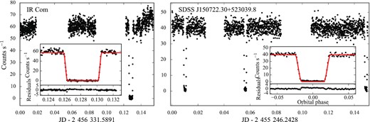
HST/COS light curves of IR Com (left) and SDSS J150722.30+523039.8 (right). The absence of any contamination from the bright spot allows us to fit the eclipse light curve and measure the mass of the white dwarf in these systems. The insets show a close-up of the eclipse of IR Com and of the average phase-folded eclipse light curve of SDSS J150722.30+523039.8, along with the best-fitting models (red).
It is worth mentioning at this point that the eclipse of the white dwarf in DW UMa was detected in the STIS time–tag data. This light curve has already been analysed by Araujo-Betancor et al. (2003), which derived a white dwarf mass of |$M_\mathrm{WD} = 0.77 \pm 0.07\, \mathrm{M_\odot }$|. Finally, DV UMa is also eclipsing but, since the data were acquired as snapshot, the light curve of the eclipse is not available.
3.2 Ultraviolet spectral fitting
To perform the spectral fit to the ultraviolet data, we generated a grid of white dwarf synthetic atmosphere models using tlusty and synspec (Hubeny 1988; Hubeny & Lanz 1995), covering the effective temperature range |$T_\mathrm{eff} = 9000 \!-\! 70\, 000\,$| K in steps of |$100\,$| K, and the surface gravity range log (g) = 6.4–9.5 in steps of 0.1 (where g is expressed in cgs units). As discussed by Pala et al. (2017), using a single metallicity is sufficient to account for the presence of the metal lines and possible deviations of single element abundances from the overall scaling with respect to the solar values do not affect the results of the fitting procedure. We therefore fixed the metal abundances to the values derived from the analysis of the same HST data by previous works (see Table 5 and references therein).
The HST ultraviolet spectra are contaminated by geocoronal emission of Ly α and O i (1302 Å). The first is always detected and we masked the corresponding wavelength range for our spectral analysis. In the case of O i, the related wavelength range was masked only when the emission was detected in the spectrum. Moreover, CV ultraviolet spectra show the presence of an additional continuum component, which contributes |$\simeq 10\!-\!30\,$| per cent of the observed flux. The origin of this additional emission source is unclear and it has been suggested that it could arise from either (i) the disc, or (ii) the hot spot where the ballistic stream intersects with the disc or (iii) the interface region between the disc and the white dwarf surface (e.g. Long et al. 1993; Godon et al. 2004; Gänsicke et al. 2005). In the literature, different approximations have been used to model the emission of this additional component, such as a blackbody, a power law or a constant flux (in Fλ). As discussed by Pala et al. (2017), these assumptions represent a very simplified model of the additional continuum contribution and it is likely that none of them provides a realistic physical description of this emission component. These authors also showed that, when only a limited wavelength coverage (|$1105\!-\!1800\,$| Å) is available, it is not possible to statistically discriminate among the three of them, and they all result in fits of similar quality for the white dwarf. We therefore decided to use a blackbody, which is described by two free parameters (a temperature and a scaling factor), because, in the limited wavelength here considered, its tail approximates both the power law and the constant flux cases.
The only exceptions are the eclipsing systems (discussed below) and GD 552. For the latter, additional data obtained with the G230L grating, covering the wavelength range |$1650\!-\!3150\,$| Å, are available. As already noticed by Unda-Sanzana et al. (2008), the additional second component in the near-ultraviolet flux of GD 552 shows a clear dependence on wavelength (orange line in Fig. 5). The observed slope could arise from either an optically thin emission region, or an optically thick accretion disc, or a bright spot. All cases are expected to display a power-law distribution (which, for the optically thick disc and the bight spot, results from the approximation with a sum of blackbodies) and, given the wide wavelength coverage available for this object, a single blackbody would represent a poor approximation for the additional emission component. Therefore, in the case of GD 552, we assumed a power-law, which is described by two free parameters (a power-law index and a scaling factor).
HST spectrum of GD 552 obtained from the combination of the STIS/G140L far-ultraviolet (blue) and STIS/G230L (black) data (the grey bands mask the geocoronal emission lines of Ly α at |$1216\,$| Å and of O i at |$1302\,$| Å, while the gaps at |$\simeq 1950\,$| Å and |$\simeq 2600\,$| Å correspond to data with bad quality flags). The best-fitting model (red) is composed of the sum of the white dwarf emission (grey), the emission lines approximated as Gaussian profiles (green), and an additional second component (orange) which shows a clear dependence on wavelength. This suggests that this additional emission component in the system is either an optically thin emission region, or an optically thick accretion disc, or a bright spot. These cases are expected to display a power-law distribution and, in our fitting procedure, we assumed a power law to model the emission of this additional component in GD 552.
The analysis of the eclipsing systems is complicated by the presence of the so-called ‘iron curtain’, i.e. a layer of absorbing material extending above the disc which gives rise to strong absorption features (see e.g. the spectrum of IY UMa in Fig. 1), mainly a forest of blended Fe ii absorption lines (Horne et al. 1994). These veil the white dwarf emission, making it difficult to establish the actual flux level (necessary to constrain the white dwarf radius). In addition, these lines modify the overall slope of the spectrum as well as the shape of the core of the Ly α line, which are the tracers for the white dwarf Teff. Out of the six eclipsing systems in our sample, two are strongly affected by the veiling gas: IY UMa and DV UMa. Following the consideration by Pala et al. (2017), in the spectral fitting of these CVs, we included two homogeneous slabs, one cold (|$T_\mathrm{curtain} \simeq 10\, 000\,$| K) and one hot (|$T_\mathrm{curtain} \simeq 80\, 000\,$| K). We generated two grids of monochromatic opacity of the slabs using synspec, one covering the effective temperature range |$T_\mathrm{eff} = 5000 \!-\! 25\, 000\,$| K and the other the range |$T_\mathrm{eff} = 25\, 000 \!-\! 120\, 000\,$| K, both in steps of 5000 K. Both grids covered the electron density range ne = 109–1021 cm−3 in steps of 103 cm−3 and the turbulence velocity range |$V_\mathrm{t} = 0\!-\!500\, \mathrm{km\, s}^{-1}$| in steps of |$100\, \mathrm{km\, s}^{-1}$|. These models, combined with the column densities (NH, for which we assumed a flat prior in the range |$10^{17} \!-\! 10^{23}\, \mathrm{cm}^{-2}$|), return the absorption due to the curtain. Given the large number of free parameters involved in the spectral fitting of the eclipsing systems, we chose to use a constant flux (in Fλ) to approximate the additional continuum component, as this is the simplest approximation and introduces only one more additional free parameter in the fitting procedure.
Finally, for all systems, whenever detected, we included the emission lines arising from the accretion disc as Gaussian profiles, allowing three free parameters: amplitude (fem), wavelength (λem), and width (σem). As shown by Pala et al. (2017), by including or masking the disc lines has no influence on the result but their inclusion allowed us to use as much of the data as possible.
We performed the spectral fit using the Markov chain Monte Carlo (MCMC) implementation for python, emcee (Foreman-Mackey et al. 2013).
We scaled the models according to the distance to the system, computed as described in Section 2.1.1, and reddened them according to the extinction values reported in Table 1. We used the STructuring by Inversion the Local Interstellar Medium (Stilism) reddening map (Lallement et al. 2018) to derive the E(B − V). For those objects not included in the Stilism reddening maps, we used instead the 3D map of interstellar dust reddening based on Pan-STARRS 1 and 2MASS photometry (Green et al. 2019).
The free parameters of the fit and their allowed range of variations are listed in Table 4, and we assumed a flat prior in the ranges covered by the corresponding grid of models. We assumed the mass–radius relation of Holberg & Bergeron (2006), Tremblay et al. (2011) and constrained the parameters describing the blackbody (BB) and constant additional second components to be positive. In the case of the power-law (PL) additional second component, we only constrained its scaling factor to be positive.
Summary of the fit parameters employed in the analysis of the ultraviolet spectra described in Section 3.2.
| System component | Parameter | Free? | Range of variation | |
|---|---|---|---|---|
| Distance | ✗ | – | ||
| E(B − V) | ✗ | – | ||
| White dwarf | |$\rm{T_\mathrm{eff}}$| (K) | |$\checkmark$| | 9000–70 000 | |
| log (g) | |$\checkmark$| | 6.4–9.5 | ||
| fem | |$\checkmark$| | >0 | ||
| Emission lines | λem | |$\checkmark$| | >0 | |
| σem | |$\checkmark$| | >0 | ||
| BB | |$\rm{T_\mathrm{eff}}$| (K) | |$\checkmark$| | >0 | |
| Second components | scaling factor | |$\checkmark$| | >0 | |
| PL | Exponent | |$\checkmark$| | |$\mathbb {R}$| | |
| scaling factor | |$\checkmark$| | >0 | ||
| constant | |$\checkmark$| | >0 | ||
| Tcurtain (K) | |$\checkmark$| | 5000–25 000 | ||
| Cold | log (ne · cm3) | |$\checkmark$| | 9–21 | |
| log (NH · cm2) | |$\checkmark$| | 17–23 | ||
| Slabs | |$V_\mathrm{t}\, (\mathrm{km\, s}^{-1})$| | |$\checkmark$| | 0–500 | |
| Tcurtain (K) | |$\checkmark$| | 25 000–120 000 | ||
| Hot | log (ne · cm3) | |$\checkmark$| | 9–21 | |
| log (NH · cm2) | |$\checkmark$| | 17–23 | ||
| |$V_\mathrm{t}\, (\mathrm{km\, s}^{-1})$| | |$\checkmark$| | 0–500 |
The accuracy derived from the statistical uncertainties are typically two and four per cent for |$\rm{T_\mathrm{eff}}$| and RWD, respectively. These uncertainties together provide an accuracy on the white dwarf masses of typically |$0.03\, \mathrm{M_\odot }$|. However, the real uncertainties are dominated by systematic effects, which are discussed in the following Section.
3.2.1 Uncertainty estimate
As discussed by Pala et al. (2017), we can rule out the presence of systematics arising from instrument flux calibration issues as well as any noticeable contamination from additional Ly α absorption from the second emission component and/or interstellar gas along the line of sight. Moreover, the uncertainties related to the unknown nature of the second component are smaller than the statistical errors from the fitting procedure (Pala et al. 2017), therefore their effect is already accounted for in the error balance from the previous Section.
The remaining sources of uncertainties are hence those related to the precision on the Gaia parallaxes and the reddening measurements. The reddening due to interstellar dust along the line of sight affects the overall slope and flux level of the observed spectrum, thus influencing both the radius and Teff measurements. Similarly, the precision on the Gaia parallax directly reflects that in the radius and hence in the white dwarf mass.
Allowing a |$3\, \sigma$| variation for both the parallax and the reddening, the observed flux level of a system could be reproduced by a combination of high reddening (i.e. more absorption along the line of sight) and a large parallax (i.e. moving the object closer to the observer) and vice versa. This degeneracy cannot be broken from the sole analysis of the HST data since they do not extend to the wavelength range where the signature of interstellar dust absorption could be detected as a bump at |$\simeq 2175\,$| Å, from which the colour excess can be estimated.
Ideally, the spectroscopic fitting procedure described in the previous section could account for this correlation by allowing both the distance and the reddening to vary according to suitable priors. In practice, this approach would require including in our fitting procedure the probability density function we used to compute the distance to each system in Section 2.1.1. Since this is not straightforward, we preferred to use an alternative method and estimate the systematic uncertainty on our mass measurements employing a Monte Carlo approach. We used a χ2 minimization routine to fit each spectrum 5000 times. During each execution, the models were scaled assuming a distance drawn randomly from the probability density function used to compute the distance to each system in Section 2.1.1. Similarly, the models were also corrected for the reddening, assuming a colour excess drawn randomly from a normal distribution, centred on the E(B − V) reported in Table 1 and weighted according to its uncertainty. Keeping the distance and the reddening fixed to the values drawn from these distributions, we allowed as free parameters the white dwarf |$\rm{T_\mathrm{eff}}$| and log (g) and the second continuum component (as defined in the previous Section). To speed up the calculation, we masked the emission lines.
From the best-fitting parameters obtained from each of the 5000 executions, we derived the posterior distribution of |$\rm{T_\mathrm{eff}}$| and log (g), which provided the estimates of the systematic uncertainties related to the accuracy on the distance and the reddening. We compared these systematics with the statistical uncertainties derived in the previous Section and assumed as final value the maximum of the two.
In the next few years, the upcoming Gaia data releases will improve the accuracy on the parallaxes, and thereby that on the distances to CVs, and will allow reconstruction of more detailed 3D reddening maps. Eventually, these will make it possible to reduce the uncertainties on the white dwarf parameters to the level of the statistical ones.
3.3 Radial velocity measurements from optical spectra
Among the different lines arising from the secondary photosphere listed in Section 2.2, the K i (|$12\, 432/12\, 522$| Å) lines are the strongest and the only ones visible in the spectra of all three systems. The Na i doublet is only visible in the spectra of IR Com but it is contaminated by the residual of the telluric line removal. Therefore, we decided not to include it in the following analysis. We used the Mg ii absorption feature and the K i lines to track the reflex motion of the white dwarf and the donor, respectively. Our data were characterized by a relatively low SNR (≃10–20 in the UVB and ≃5 in the NIR) and, moreover, the NIR spectra showed strong contamination from the residuals from the sky lines subtraction. Therefore, to achieve more robust radial velocity measurements, we fit all the spectra of each object simultaneously (as done e.g. by Parsons et al. 2012 and Pala et al. 2019).
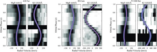
For each system, the trailed spectra for the Mg ii line (4481 Å, left-hand panel) and the K i line (|$12\, 522$| Å, right-hand panel) are shown. Overplotted are the best-fitting models (red) along with their uncertainties (light blue).
By assuming the same mass–radius relationship as in Section 3.1.1 and using equation (5), we measured the masses of the three CV white dwarfs, which result in |$0.76^{+0.06}_{-0.07}$|, |$0.95\pm 0.04$|, and |$0.91^{+0.14}_{-0.20}\, \mathrm{M_\odot }$|, for AX For, IR Com, and V1108 Her, respectively (Table 6). In Section 4.1.3, we discuss these results in comparison with the masses obtained from the analysis of the ultraviolet spectra.
The accuracy we achieved on these measurements is directly related to the quality of the data. An optimal sampling of the orbital period is crucial to precisely measure radial velocities. This can be seen by comparing the results for IR Com with those for AX For and V1108 Her. The data of the former are almost evenly distributed along the orbital period and allow us to obtain accuracy of the order ≃7 per cent. However, the observations of AX For were affected by clouds while those of V1108 Her were contaminated by the presence of a close background star. In both cases, we were forced to reject some spectra, resulting in poor orbital sampling and larger uncertainties.
3.4 Summary on the mass measurements
The results of our fitting procedures are summarized in Table 5. In the case of the white dwarf in AX For, from the analysis of the ultraviolet data, we derived a smaller radius (|$\simeq 0.0142\, \mathrm{R_\odot }$|) than the one estimated from the gravitational redshift (|$\simeq 0.0190\, \mathrm{R_\odot }$|). We can thus roughly estimate that at the time of the HST observations |$\simeq 77\,$| per cent of the white dwarf surface was still heated by the recent outburst and, therefore, we assumed as final measurements for its mass and radius those obtained from the gravitational redshift in Section 3.3.
White dwarf parameters and mass accretion rates for the 42 CVs observed with HST during their quiescent state and for AX For, whose radius and mass have been obtained from the white dwarf gravitational redshift.
| System | |$\rm{P_\mathrm{orb}}$| | d | Z | References | |$\rm{T_\mathrm{eff}}$| | RWD | MWD | log (g) | |$\langle \dot{M} \rangle$| | White dwarf |
|---|---|---|---|---|---|---|---|---|---|---|
| (min) | (pc) | Z⊙ | (K) | (|$0.01\, \mathrm{R}_\odot$|) | (M⊙) | |$(10^{-10}\, \mathrm{M}_\odot$| yr−1) | contribution (per cent) | |||
| SDSS J150722.30+523039.8 | 66.61 | 211 ± 4 | 0.1 | 1 | |$14\, 207^{+356}_{-403}$| | |$0.93^{+0.17}_{-0.12}$| | |$0.90^{+0.10}_{-0.14}$| | |$8.45^{+0.16}_{-0.22}$| | |$0.53^{+0.18}_{-0.11}$| | 78 |
| SDSS J074531.91+453829.5 | 76.0 | |$310^{+23}_{-20}$| | 0.1 | 2 | |$15\, 447^{+556}_{-654}$| | |$1.1^{+0.3}_{-0.2}$| | |$0.75^{+0.18}_{-0.20}$| | |$8.2^{+0.3}_{-0.4}$| | |$1.2^{+0.7}_{-0.4}$| | 88 |
| GW Lib | 76.78 | 112.6 ± 0.8 | 0.2 | 3 | |$16\, 166^{+253}_{-350}$| | |$1.03^{+0.15}_{-0.1}$| | |$0.83^{+0.08}_{-0.12}$| | |$8.33^{+0.13}_{-0.18}$| | |$1.12^{+0.32}_{-0.19}$| | 86 |
| SDSS J143544.02+233638.7 | 78.0 | |$208^{+9}_{-8}$| | 0.01 | 3 | |$11\, 997^{+99}_{-160}$| | |$1.00^{+0.08}_{-0.09}$| | |$0.84^{+0.07}_{-0.06}$| | |$8.36^{+0.11}_{-0.1}$| | |$0.32^{+0.08}_{-0.05}$| | 90 |
| OT J213806.6+261957 | 78.1 | 98.9 ± 0.4 | 0.2 | 3 | |$15\, 317^{+216}_{-228}$| | |$1.39^{+0.15}_{-0.12}$| | |$0.57^{+0.06}_{-0.07}$| | |$7.91^{+0.12}_{-0.15}$| | |$1.9^{+0.4}_{-0.3}$| | 73 |
| BW Scl | 78.23 | 93.4 ± 0.5 | 0.5 | 4 | |$15\, 145^{+51}_{-57}$| | |$0.8^{+0.014}_{-0.011}$| | |$1.007^{+0.010}_{-0.012}$| | |$8.635^{+0.017}_{-0.02}$| | |$0.483^{+0.014}_{-0.012}$| | 87 |
| LL And | 79.28 | |$609^{+343}_{-205}$| | 1.0 | 5 | |$14\, 353^{+1210}_{-743}$| | |$1.2^{+0.8}_{-0.6}$| | |$0.7^{+0.4}_{-0.3}$| | 8.2 ± 0.7 | |$0.9^{+2.4}_{-0.9}$| | 80 |
| AL Com | 81.6 | |$523^{+252}_{-149}$| | 0.2 | 6 | |$15\, 840^{+1453}_{-1243}$| | |$1.0^{+0.9}_{-0.6}$| | |$0.9^{+0.5}_{-0.3}$| | 8.4 ± 0.8 | |$0.9^{+3.1}_{-1.0}$| | 79 |
| WZ Sge | 81.63 | 45.17 ± 0.06 | 0.01 | 7 | |$13\, 190^{+115}_{-105}$| | 1.05 ± 0.03 | 0.8 ± 0.02 | 8.3 ± 0.04 | |$0.52^{+0.014}_{-0.01}$| | 78 |
| SW UMa | 81.81 | |$160.6^{+1.6}_{-1.5}$| | 0.2 | 4 | |$13\, 854^{+189}_{-131}$| | |$1.29^{+0.09}_{-0.10}$| | |$0.61^{+0.06}_{-0.04}$| | |$8.01^{+0.11}_{-0.09}$| | |$1.07^{+0.15}_{-0.14}$| | 61 |
| V1108 Her | 81.87 | 148 ± 2 | 1.0 | 3 | |$13\, 943^{+185}_{-226}$| | |$0.95^{+0.14}_{-0.11}$| | |$0.88^{+0.09}_{-0.11}$| | |$8.42^{+0.15}_{-0.17}$| | |$0.52^{+0.15}_{-0.11}$| | 75 |
| ASAS J002511+1217.2 | 82.0 | 157 ± 3 | 0.1 | 3 | |$13\, 208^{+154}_{-112}$| | 0.78 ± 0.04 | 1.02 ± 0.04 | 8.66 ± 0.07 | |$0.27^{+0.03}_{-0.02}$| | 74 |
| HV Vir | 82.18 | |$317^{+29}_{-25}$| | 0.2 | 8 | |$12\, 958^{+257}_{-291}$| | |$0.96^{+0.21}_{-0.16}$| | |$0.87^{+0.13}_{-0.17}$| | |$8.4^{+0.2}_{-0.3}$| | |$0.4^{+0.2}_{-0.12}$| | 93 |
| SDSS J103533.02+055158.4 | 82.22 | |$195^{+12}_{-10}$| | 0.01 | 3 | |$11\, 876^{+108}_{-115}$| | |$0.8^{+0.11}_{-0.09}$| | |$1.00^{+0.08}_{-0.10}$| | |$8.63^{+0.14}_{-0.16}$| | |$0.18^{+0.06}_{-0.04}$| | 91 |
| WX Cet | 83.9 | |$252^{+9}_{-8}$| | 0.1 | 9 | |$15\, 186^{+1460}_{-1468}$| | |$0.63^{+0.28}_{-0.18}$| | |$1.10^{+0.17}_{-0.21}$| | 8.8 ± 0.4 | |$0.3^{+0.07}_{-0.06}$| | 24 |
| SDSS J075507.70+143547.6 | 84.76 | |$239^{+12}_{-11}$| | 0.5 | 3 | |$16\, 193^{+280}_{-357}$| | |$0.92^{+0.15}_{-0.11}$| | |$0.91^{+0.09}_{-0.12}$| | |$8.47^{+0.15}_{-0.19}$| | |$0.87^{+0.27}_{-0.18}$| | 87 |
| SDSS J080434.20+510349.2 | 84.97 | 142 ± 2 | 0.5 | 10 | |$13\, 715^{+55}_{-79}$| | |$0.80^{+0.04}_{-0.03}$| | |$1.01^{+0.03}_{-0.04}$| | |$8.64^{+0.05}_{-0.06}$| | 0.32 ± 0.03 | 87 |
| EK TrA | 86.36 | 151.4 ± 0.8 | 0.5 | 11 | |$17\, 608^{+269}_{-481}$| | |$0.97^{+0.17}_{-0.11}$| | |$0.87^{+0.09}_{-0.13}$| | |$8.4^{+0.14}_{-0.21}$| | |$1.4^{+0.4}_{-0.3}$| | 58 |
| EG Cnc | 86.36 | 186 ± 7 | 0.2 | 8 | |$12\, 295^{+56}_{-57}$| | |$0.77^{+0.06}_{-0.05}$| | |$1.03^{+0.04}_{-0.05}$| | |$8.67^{+0.07}_{-0.08}$| | |$0.2^{+0.03}_{-0.02}$| | 100 |
| 1RXS J105010.8–140431 | 88.56 | |$108.9^{+1.1}_{-1.0}$| | 0.1 | 3 | |$11\, 523^{+29}_{-47}$| | |$1.08^{+0.04}_{-0.03}$| | |$0.77^{+0.02}_{-0.03}$| | |$8.25^{+0.04}_{-0.05}$| | |$0.332^{+0.028}_{-0.018}$| | 87 |
| BC UMa | 90.16 | |$293^{+11}_{-10}$| | 0.2 | 4 | |$14\, 378^{+272}_{-327}$| | |$1.57^{+0.19}_{-0.16}$| | |$0.48^{+0.08}_{-0.09}$| | |$7.73^{+0.15}_{-0.19}$| | |$2.0^{+0.5}_{-0.3}$| | 85 |
| VY Aqr | 90.85 | |$141.3^{+1.9}_{-1.8}$| | 0.5 | 9 | |$14\, 453^{+316}_{-366}$| | |$0.74^{+0.07}_{-0.06}$| | 1.06 ± 0.06 | |$8.73^{+0.12}_{-0.11}$| | |$0.33^{+0.04}_{-0.03}$| | 45 |
| QZ Lib | 92.36 | |$199^{+11}_{-10}$| | 0.01 | 3 | |$11\, 419^{+175}_{-229}$| | |$1.01^{+0.23}_{-0.18}$| | |$0.82^{+0.14}_{-0.19}$| | |$8.3^{+0.2}_{-0.3}$| | |$0.27^{+0.15}_{-0.09}$| | 74 |
| SDSS J153817.35+512338.0 | 93.11 | |$607^{+47}_{-40}$| | 0.01 | 3 | |$35\, 284^{+600}_{-688}$| | |$0.89^{+0.16}_{-0.12}$| | |$0.97^{+0.09}_{-0.11}$| | |$8.53^{+0.17}_{-0.2}$| | |$18.0^{+7.0}_{-4.0}$| | 100 |
| UV Per | 93.44 | |$248^{+7}_{-6}$| | 0.2 | 3 | |$14\, 040^{+539}_{-645}$| | |$1.2^{+0.4}_{-0.3}$| | 0.7 ± 0.2 | 8.1 ± 0.4 | |$0.9^{+0.7}_{-0.4}$| | 69 |
| 1RXS J023238.8–371812 | 95.04 | |$214^{+8}_{-7}$| | 0.2 | 3 | |$14\, 457^{+118}_{-135}$| | |$0.63^{+0.05}_{-0.04}$| | 1.15 ± 0.04 | |$8.9^{+0.07}_{-0.08}$| | 0.23 ± 0.03 | 71 |
| RZ Sge | 98.32 | 294 ± 7 | 0.5 | 3 | |$15\, 197^{+419}_{-507}$| | |$1.09^{+0.27}_{-0.17}$| | |$0.78^{+0.13}_{-0.18}$| | |$8.3^{+0.2}_{-0.3}$| | |$1.0^{+0.5}_{-0.3}$| | 51 |
| CY UMa | 100.18 | 306 ± 6 | 0.1 | 3 | |$14\, 692^{+471}_{-394}$| | 1.40 ± 0.13 | |$0.57^{+0.08}_{-0.06}$| | |$7.91^{+0.14}_{-0.13}$| | 1.6 ± 0.2 | 63 |
| GD 552 | 102.73 | 80.6 ± 0.2 | 0.1 | 12 | |$10\, 761^{+37}_{-43}$| | |$1.07^{+0.05}_{-0.04}$| | |$0.78^{+0.03}_{-0.04}$| | |$8.27^{+0.05}_{-0.06}$| | |$0.243^{+0.023}_{-0.018}$| | 55 |
| IY UMa* | 106.43 | 181 ± 2 | 1.0 | 3 | |$17\, 057^{+179}_{-79}$| | |$0.83^{+0.04}_{-0.05}$| | |$0.99^{+0.04}_{-0.03}$| | |$8.59^{+0.07}_{-0.05}$| | 0.85 ± 0.07 | 79 |
| SDSS J100515.38+191107.9 | 107.6 | |$339^{+21}_{-19}$| | 0.2 | 3 | |$14\, 483^{+520}_{-430}$| | |$1.7^{+0.4}_{-0.3}$| | |$0.44^{+0.15}_{-0.09}$| | 7.6 ± 0.3 | |$2.4^{+1.2}_{-0.8}$| | 76 |
| RZ Leo | 110.17 | |$279^{+12}_{-11}$| | 0.5 | 3 | |$15\, 573^{+437}_{-424}$| | |$0.85^{+0.2}_{-0.16}$| | |$0.97^{+0.13}_{-0.16}$| | |$8.6^{+0.2}_{-0.3}$| | |$0.62^{+0.3}_{-0.19}$| | 81 |
| CU Vel | 113.04 | 158.5 ± 1.1 | 0.1 | 3 | |$14\, 174^{+117}_{-169}$| | |$1.58^{+0.11}_{-0.08}$| | |$0.47^{+0.04}_{-0.05}$| | |$7.71^{+0.08}_{-0.11}$| | |$1.97^{+0.28}_{-0.19}$| | 90 |
| AX For | 113.04 | 349 ± 10 | 1.0 | 3 | – | |$1.09^{+0.08}_{-0.09}$| | 0.76 ± 0.07 | 8.24 ± 0.08 | – | – |
| EF Peg | 120.53 | |$288^{+21}_{-18}$| | 0.2 | 5 | |$16\, 644^{+448}_{-570}$| | 1.1 ± 0.2 | |$0.8^{+0.16}_{-0.17}$| | 8.3 ± 0.3 | |$1.3^{+0.5}_{-0.4}$| | 90 |
| DV UMa* | 123.62 | |$382^{+24}_{-21}$| | 1.0 | 3 | |$19\, 410^{+244}_{-400}$| | |$0.86^{+0.12}_{-0.09}$| | |$0.96^{+0.07}_{-0.1}$| | |$8.55^{+0.13}_{-0.16}$| | |$1.5^{+0.4}_{-0.3}$| | 89 |
| IR Com | 125.34 | 216 ± 3 | 1.0 | 3 | |$17\, 531^{+236}_{-271}$| | |$0.78^{+0.11}_{-0.08}$| | |$1.03^{+0.07}_{-0.09}$| | |$8.67^{+0.12}_{-0.15}$| | |$0.82^{+0.21}_{-0.15}$| | 87 |
| AM Her | 185.65 | 87.9 ± 0.2 | 0.001 | 13 | |$19\, 248^{+486}_{-450}$| | |$1.3^{+0.17}_{-0.14}$| | |$0.63^{+0.1}_{-0.08}$| | |$8.01^{+0.17}_{-0.16}$| | |$4.0^{+0.9}_{-0.7}$| | 92 |
| DW UMa | 196.71 | |$579^{+7}_{-6}$| | 0.71 | 14 | |$56\, 760^{+146}_{-259}$| | |$1.19^{+0.07}_{-0.05}$| | |$0.82^{+0.03}_{-0.04}$| | |$8.2^{+0.05}_{-0.07}$| | 228.0 ± 24.0 | 97 |
| U Gem | 254.74 | 93.0 ± 0.3 | 1.0 | 15 | |$33\, 070^{+648}_{-616}$| | 0.634 ± 0.016 | 1.160 ± 0.013 | 8.90 ± 0.03 | |$6.53^{+0.22}_{-0.17}$| | 100 |
| SS Aur | 263.23 | |$249.0^{+1.8}_{-1.7}$| | 0.1 | 16 | |$28\, 627^{+190}_{-269}$| | |$0.86^{+0.15}_{-0.11}$| | |$0.98^{+0.09}_{-0.11}$| | |$8.56^{+0.16}_{-0.19}$| | |$7.3^{+3.0}_{-1.9}$| | 100 |
| RX And | 302.25 | 196.7 ± 1.0 | 0.5 | 17 | |$33\, 900^{+634}_{-995}$| | |$1.12^{+0.12}_{-0.08}$| | |$0.81^{+0.06}_{-0.08}$| | |$8.25^{+0.1}_{-0.13}$| | |$26.0^{+6.0}_{-4.0}$| | 100 |
| V442 Cen | 662.4 | 343 ± 5 | 0.01 | 16 | |$29\, 802^{+211}_{-247}$| | |$1.35^{+0.14}_{-0.12}$| | |$0.64^{+0.06}_{-0.05}$| | 7.98 ± 0.12 | |$25.0^{+5.0}_{-4.0}$| | 100 |
Notes. For each object, its orbital period and metallicity are compiled from the literature. The last five columns report the results from this work. The two systems highlighted with a star are those for which the curtain of veiling gas has been detected in their ultraviolet spectra.
References. (1) Uthas et al. (2011), (2) Mukadam et al. (2013), (3) Pala et al. (2017), (4) Gänsicke et al. (2005), (5) Howell et al. (2002), (6) Szkody et al. (2003), (7) Sion et al. (1995), (8) Szkody et al. (2002a), (9) Sion et al. (2003), (10) Szkody et al. (2013), (11) Gänsicke et al. (2001), (12) Unda-Sanzana et al. (2008), (13) Gänsicke et al. (2006), (14) Araujo-Betancor et al. (2003), (15) Cheng et al. (1997), (16) Sion et al. (2008), and (17) Sion et al. (2001).
We show in Fig. 7 some examples of best-fitting models for three non-eclipsing systems in different temperature regimes, and for an eclipsing CV. All spectra, along with their best-fitting models, are available in Section 2 of the online material.
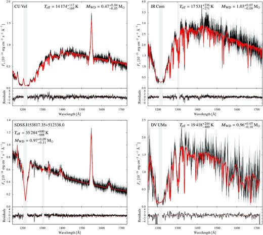
Ultraviolet spectra (black) of sample CV white dwarfs along with the best-fitting model (red), representative of cool (top left panel), warm (top right panel), hot (bottom left panel), and eclipsing (bottom right panel) systems. The best-fitting models are composed of the sum of a white dwarf synthetic atmosphere model, a second continuum emission component in the form of a blackbody, and the emission lines from the disc modelled with a Gaussian profile. In addition, the model for the eclipsing system DV UMa (bottom right) includes an ‘absorption curtain’ component (see Section 3.2). The grey bands mask the geocoronal emission lines of Ly α (|$1216\,$| Å) and, whenever present, of O i (|$1302\,$| Å).
4 DISCUSSION
4.1 Comparison with previous mass measurements and different techniques
4.1.1 Eclipsing systems
Previous mass measurements from the analysis of the eclipse light curve of the white dwarf were obtained from optical observations for DV UMa, IY UMa, SDSS J103533.02+055158.4, and SDSS J150722.30+523039.8 (Savoury et al. 2011; McAllister et al. 2019), and from ultraviolet observations for DW UMa (Araujo-Betancor et al. 2003). Moreover, we here derived a mass measurement for IR Com and SDSS J150722.30+523039.8 from the analysis of their ultraviolet light curves (Section 3.1.1). We find a good agreement (within 3σ, Table 6 and Fig. 8) between the masses derived employing the two different methods (ultraviolet spectral fit versus analysis of the white dwarf eclipse).
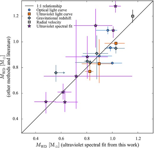
Comparison between the CV white dwarf masses derived in this work from the analysis of the ultraviolet HST spectra and those obtained employing other methods and from the analysis of the same ultraviolet data in the literature. The error bars show the corresponding 1σ uncertainties.
Summary of the CV white dwarf masses derived in this work from the analysis of the ultraviolet data and those obtained employing other methods. The systems are sorted by increasing masses.
| MWD (M⊙) | |||||||
|---|---|---|---|---|---|---|---|
| System | Ultraviolet | Ultraviolet | Ultraviolet | Optical | Gravitational | Radial | References |
| spectral fit | spectral fit | light curve | light curve | redshift | velocities | ||
| (this work) | (literaturea) | ||||||
| BC UMa | |$0.48^{+0.08}_{-0.09}$| | |$0.53^{+0.07}_{-0.09}$| | – | – | – | – | Gänsicke et al. (2005) |
| AX For | 0.56↑ | – | – | – | |$0.76^{+0.06}_{-0.07}$| | – | This work |
| SW UMa | |$0.61^{+0.06}_{-0.04}$| | 0.61 ± 0.6 | – | – | – | – | Gänsicke et al. (2005) |
| AM Her | |$0.63^{+0.10}_{-0.08}$| | |$0.53^{+0.10}_{-0.08}$| | – | – | – | – | Gänsicke et al. (2006) |
| LL And | |$0.7^{+0.4}_{-0.3}$| | |$0.7^{+0.4}_{-0.3}$| | – | – | – | – | Howell et al. (2002) |
| EF Peg | |$0.80^{+0.16}_{-0.17}$| | |$0.88^{+0.16}_{-0.17}$| | – | – | – | – | Howell et al. (2002) |
| WZ Sge | 0.80 ± 0.02 | – | – | – | 0.85 ± 0.04 | – | Steeghs et al. (2007) |
| DW UMa | |$0.82^{+0.03}_{-0.04}$| | – | 0.77 ± 0.07 | – | – | – | Araujo-Betancor et al. (2003) |
| GW Lib | |$0.83^{+0.08}_{-0.12}$| | – | – | – | 0.84 ± 0.02 | – | van Spaandonk et al. (2010) |
| SDSS J150722.30+523039.8 | |$0.90^{+0.10}_{-0.14}$| | – | |$0.83^{+0.19}_{-0.15}$| | 0.89 ± 0.01 | – | – | Ultraviolet light curve, this work; |
| optical light curve (Savoury et al. 2011) | |||||||
| V1108 Her | |$0.88^{+0.09}_{-0.11}$| | – | – | – | |$0.91^{+0.14}_{-0.20}$| | – | This work |
| DV UMa | |$0.96^{+0.07}_{-0.10}$| | – | – | 1.09 ± 0.03 | – | – | McAllister et al. (2019) |
| IY UMa | |$0.99^{+0.04}_{-0.03}$| | – | – | |$0.955^{+0.013}_{-0.028}$| | – | – | McAllister et al. (2019) |
| SDSS J103533.02+055158.4 | |$1.00^{+0.08}_{-0.10}$| | – | – | 0.835 ± 0.009 | – | – | Savoury et al. (2011) |
| BW Scl | |$1.007^{+0.01}_{-0.012}$| | |$1.10^{+0.03}_{-0.06}$| | – | – | – | – | Gänsicke et al. (2005) |
| IR Com | |$1.03^{+0.07}_{-0.09}$| | – | 0.989 ± 0.003 | – | 0.95 ± 0.04 | – | This work |
| U Gem | 1.16 ± 0.013 | – | – | – | – | 1.2 ± 0.05 | Echevarría, de la Fuente & Costero (2007) |
| HV Vir | |$0.87^{+0.13}_{-0.17}$| | |$1.27^{+0.13}_{-0.17}$| | – | – | – | – | Szkody et al. (2002a) |
| EG Cnc | |$1.03^{+0.04}_{-0.05}$| | |$1.28^{+0.04}_{-0.05}$| | – | – | – | – | Szkody et al. (2002a) |
The reported values have been corrected accounting for the temperature dependency of the mass-radius relationship and the reddening, as discussed in Section 4.1.2.
4.1.2 Systems with previous mass measurements from ultraviolet analysis
For several systems in our sample (AM Her, BC UMa, BW Scl, EF Peg, EG Cnc, HV Vir, LL And, and SW UMa), a mass estimate derived from the analysis of their ultraviolet HST data is available in the literature. However, these studies lacked the knowledge of the distance to the systems and therefore did not provide a single mass estimate but a range of possible values, computed assuming different distances. The method employed is described in detail by Gänsicke et al. (2005) and consists of fitting the ultraviolet data by stepping through a grid of atmosphere models with fixed values for log (g), leaving the temperature and scaling factor free. In this way, it is possible to investigate the correlation between the assumed log (g) (i.e. the white dwarf mass under the assumption of a mass–radius relationship) and the best-fitting value for Teff (see e.g. fig. 3 from Gänsicke et al. 2005) for different distances.
We retrieved the log (g)-distance correlations for AM Her, BC UMa, BW Scl, EF Peg, EG Cnc, HV Vir, LL And, and SW UMa from the works by Howell et al. (2002), Szkody et al. (2002a), and Gänsicke et al. (2005, 2006). We applied a correction to account for the dependency of the mass–radius relationship on the white dwarf Teff and for the reddening (see Section 3 of the online material for the details), which were not accounted for by these studies, and estimated the mass of the white dwarf assuming their distances from Gaia EDR3 (as described in Section 2.1.1). We computed the associated error bars by assuming a typical statistical uncertainty on the white dwarf temperature (for a fixed log (g)) of |$\simeq 200\,$| K (Gänsicke, private communications). For each object, we compared them with the systematic uncertainties derived in Section 3.2.1 (which are representative of the typical uncertainties related to the accuracy of the reddening and distance) and assumed as final uncertainties the larger between the two values. The final results are listed in Table 6 and shown in Fig. 8.
With the exception of EG Cnc, the results from the literature are in good agreement with ours within the uncertainties. The origin of the disagreement in the case of EG Cnc is not easy to unveil and could possibly be related to the different atmosphere models used by Szkody et al. (2002a), which were generated with an older version of tlusty (# 195) than the one that we used (# 204n). The most relevant differences between the two versions are an improved treatment of H|$_2^{+}$| quasi-molecular absorption lines (dominant in this cool CV) and of the Stark-broadening profiles using the calculation by Tremblay & Bergeron (2009). Therefore, we consider our results more reliable and representative of the observed flux emission of EG Cnc.
4.1.3 Systems with radial velocity measurements
For three systems in our sample, AX For, IR Com, and V1108 Her, we derived an independent mass measurement from the white dwarf gravitational redshift (Section 3.3). Moreover, additional mass measurements, which have been determined from the gravitational redshift of the white dwarfs in GW Lib (van Spaandonk et al. 2010) and WZ Sge (Steeghs et al. 2007), and from the radial velocities of the two stellar components in U Gem (Echevarría et al. 2007), are available in the literature (see also table 44 of the online material and references therein). These masses are all in good agreement with those we derived from the spectral fit to the ultraviolet data (Table 6 and Fig. 8).
4.2 Comparison with Zorotovic et al. (2011)
Fig. 9 shows the comparison between the 43 mass measurement from this work and the compilation from Zorotovic et al. (2011), which includes 22 masses derived from the analysis of the white dwarf eclipses and 10 measurements from spectroscopic studies. The two samples have eight systems in common (AM Her, DV UMa, DW UMa, IY UMa, SDSS J103533.02+055158.4, SDSS J150722.30+523039.8, U Gem, and WZ Sge, see Table 6) and this partial overlap highlights possible differences associated with the different methods employed to measure the masses of the white dwarfs.
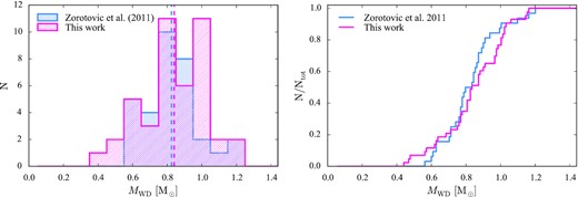
Comparison between the mass distributions (left) and the cumulative distributions (right) of the 43 white dwarfs from this work (pink) and the 32 measurements compiled by Zorotovic et al. (2011, blue). The dashed vertical lines correspond to the average masses. Our results show the presence of a tail extending to low masses corresponding to helium-core white dwarfs, which is not detected in the sample studied by Zorotovic et al. (2011).
The mass distribution we derived presents a tail extending towards low masses, consisting of three systems (BC UMa, CU Vel, and SDSS J100515.38+191107.9) with |$M_\mathrm{WD} \lt 0.5\, \mathrm{M_\odot }$|. Such low masses are consistent with either He core or, possibly, hybrid CO/He core white dwarfs. In contrast, the sample studied by Zorotovic et al. (2011) does not contain any white dwarf with |$M_\mathrm{WD} \lt 0.5\, \mathrm{M_\odot }$| although, from evolutionary considerations, they estimated that CV helium-core white dwarfs should represent |$\lesssim 10\,$| per cent of the systems.
For both distributions, we determined the average white dwarf mass 〈MWD〉 and the corresponding uncertainties as the 16th and the 84th percentiles, obtaining |$\langle M_\mathrm{WD} \rangle = 0.82 \pm 0.12\, \mathrm{M_\odot }$| for the values from Zorotovic et al. (2011) and |$\langle M_\mathrm{WD} \rangle = 0.84^{+0.18}_{-0.23}$| for the masses here derived. The agreement between these values allows us to rule out the presence of any systematics affecting the masses derived from the analysis of eclipse light curves.
4.3 The mass distribution of CV white dwarfs
Since the work by Zorotovic et al. (2011), more mass measurements of CV white dwarfs have been made available in the literature, mainly thanks to the systematic observations of eclipsing systems (e.g. Feline et al. 2005; Littlefair et al. 2006; Savoury et al. 2011; McAllister et al. 2019) with the fast triple-beam camera ULTRACAM (Dhillon et al. 2007). A more comprehensive and up-to-date census of masses in the literature consists of 54 measurements (see table 44 of the online material and reference therein), eight of which (AM Her, DV UMa, DW UMa, SDSS J103533.02+055158.4, SDSS J150722.30+523039.8, U Gem WZ Sge, and IY UMa, see Table 6) are in common with our sample. For these systems, we here assume the white dwarf parameters obtained in this work. Of the remaining 46 CV white dwarf masses from the literature, 34 have been derived from the analysis of the eclipse light curves of the white dwarf and 12 from spectroscopic studies.
Combining these 46 measurements with our results, we obtained a sample of 89 CV white dwarfs with an accurate mass, and the corresponding average mass results |$\langle M_\mathrm{WD} \rangle = 0.81^{+0.16}_{-0.20}\, \mathrm{M_\odot }$| (Fig. 10). As demonstrated by Zorotovic et al. (2011), this high average mass of CV white dwarfs cannot be ascribed to an observational bias since the detection of massive white dwarfs is disfavoured by the fact that they have smaller radii and are less luminous than low mass white dwarfs for the same |$\rm{T_\mathrm{eff}}$|. This confirms the earlier results that CV white dwarfs are genuinely more massive than predicted by most models of CV evolution, which only account for orbital angular momentum losses arising from magnetic braking and gravitational wave radiation.
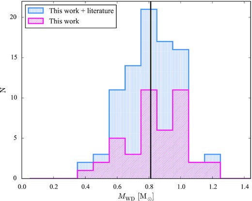
Mass distribution for the sample of 89 CV white dwarfs obtained combining the 43 mass measurements from this work (shown in pink) with the 46 from the literature. The black vertical line corresponds to the average mass of the total sample of 89 systems, |$\langle M_\mathrm{WD} \rangle = 0.81^{+0.16}_{-0.20}\, \mathrm{M_\odot }$|.
Among the systems from the literature, two (HY Eri and KIC 5608384) have |$M_\mathrm{WD} \lt 0.5\, \mathrm{M_\odot }$|. These, combined with the three low-mass primaries likely representative of He-core white dwarfs we have identified, bring the total census to five systems. On the one hand, compared to the standard models for CV evolution, the number of observed He-core white dwarfs is still far lower than predicted (e.g. |$\simeq 53\,$| per cent, Politano 1996 and |$\simeq 30\,$| per cent, Goliasch & Nelson 2015 of the present-day CV population). On the other hand, more modern scenarios that take into account a mass dependent consequential angular momentum loss and that can reproduce the overall white dwarf mass distribution in CVs do not predict any He-core white dwarfs (e.g. Schreiber et al. 2016), which is also in contrast with the observations. Our result shows that CVs hosting low-mass white dwarfs contribute to the overall CV population and that their non-zero fraction should be properly taken into account in the modelling of CV evolution.
4.4 Orbital period dependecy
While losing orbital angular momentum, CVs evolve from long to short orbital periods and, by comparing the average mass of the white dwarfs in long (|$\rm{P_\mathrm{orb}} \gt 3\,$|h) and short (|$\rm{P_\mathrm{orb}} \lt 3\,$|h) period CVs, we can investigate possible overall variations (due to either mass growth or mass erosion) with time. We do not find any difference between the average white dwarfs mass of long (|$\langle M_\mathrm{WD} \rangle = 0.80^{+0.17}_{-0.19}\, \mathrm{M_\odot }$|) and short (|$\langle M_\mathrm{WD} \rangle = 0.81^{+0.17}_{-0.16}\, \mathrm{M_\odot }$|) period CVs. Moreover, by performing an F-test on the best linear fit to the masses as a function of the orbital period, we derive an F-statistic F0 = 2.22 with p-value = 0.23 and therefore we do not find any evidence for a clear dependency on the white dwarf mass with the orbital period (Fig. 11). Nonetheless, only 21 long period CVs have mass determinations (in contrast to the 68 systems at short orbital periods) and additional measurements at long orbital periods are required to further constrain any correlation.
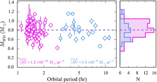
White dwarf masses from this work (circles) and from the literature (diamonds), as a function of their orbital periods. Long period (|$\rm{P_\mathrm{orb}} \gt 3\,$| h) and short (|$\rm{P_\mathrm{orb}} \lt 3\,$| h) period CVs are shown in blue and pink, respectively. The right-hand panel shows the corresponding distributions and the corresponding average masses (dashed lines), colour coded as in the left-hand panel. Note that long period CVs have, on average, secular mass accretion rates about one order of magnitude higher compared to those of short period CVs, as reported in the figure.
4.5 Mass accretion rates and CV evolution
The evolution of CVs is dictated by orbital angular momentum losses, which continuously shrink the orbit and keep the secondary in touch with its Roche lobe, ensuring the stability of the mass transfer process. For systems with |$\rm{P_\mathrm{orb}} \gtrsim 3\,$| h, the main mechanisms of angular momentum loss are magnetic wind braking and gravitational wave radiation. As the system loses orbital angular momentum, the two stellar components spiral inwards and the system evolves towards short orbital periods, while the donor star is constantly stripped of more and more mass. At |$\rm{P_\mathrm{orb}} \simeq 3\, \mathrm{h}$|, the donor star has become fully convective and, in the frequently referenced interrupted magnetic braking scenario (Paczynski & Sienkiewicz 1983; Rappaport, Verbunt & Joss 1983; Spruit & Ritter 1983), a re-configuration of the magnetic fields takes place on the donor, leading to a great reduction in the efficiency of magnetic braking. As a consequence, the secondary star detaches from its Roche lobe and, in the period range |$2\, \mathrm{h} \lesssim \rm{P_\mathrm{orb}} \lesssim 3\,$|h (the so-called period gap) the system evolves as a detached binary whilst still losing angular momentum through gravitational wave radiation. Accretion then resumes at |$\rm{P_\mathrm{orb}} \simeq 2\,$| h, when the orbital separation brings again the donor in contact with its Roche lobe, and the system keep evolving towards shorter orbital periods. When the system reaches the ‘period minimum’ at |$\rm{P_\mathrm{orb}} \simeq 80\, \mathrm{min}$|, the time-scale on which the secondary star loses mass becomes much shorter than its thermal time-scale and the secondary stops shrinking in response to the mass-loss. Consequently, systems that have passed the period minimum evolve back towards longer orbital periods and, for this reason, are called ‘period bouncers’.
The different efficiencies of magnetic braking and gravitational wave radiation in removing angular momentum from the binary orbit cause long period CVs to have |$\langle \dot{M}\rangle$| about one order of magnitude higher compared to those of short period CVs. Determining the rate of angular momentum loss is therefore important in order to test the models of CV evolution. However, a direct measurement via detection of orbital period changes is impossible on human time-scales. A very good proxy for the angular momentum loss rate is the white dwarf effective temperature (Townsley & Bildsten 2003), as it is determined by the compressional heating of the accreted material (Sion 1995; Townsley & Bildsten 2004). Therefore, |$\rm{T_\mathrm{eff}}$| provides a constraint on the mean mass-accretion rate |$\langle \dot{M} \rangle$|, averaged over the thermal time-scale of the white dwarf envelope (|$10^3\!-\!10^5\,$| yr), which is a direct measurement of the angular momentum loss rate in the system (Townsley & Gänsicke 2009).
Fig. 12 shows the effective temperatures (top) and the mass accretion rates (bottom) as a function of the orbital period for 65 systems, 41 from our HST sample9 (circles and stars) and 34 from the literature (diamonds and pentagons), for which both |$\rm{T_\mathrm{eff}}$| and MWD are available. We find that systems above the gap are hotter and accrete at higher rates than systems below the gap, reflecting the different rates of angular momentum loss driving the evolution of these binaries in different orbital period regimes.
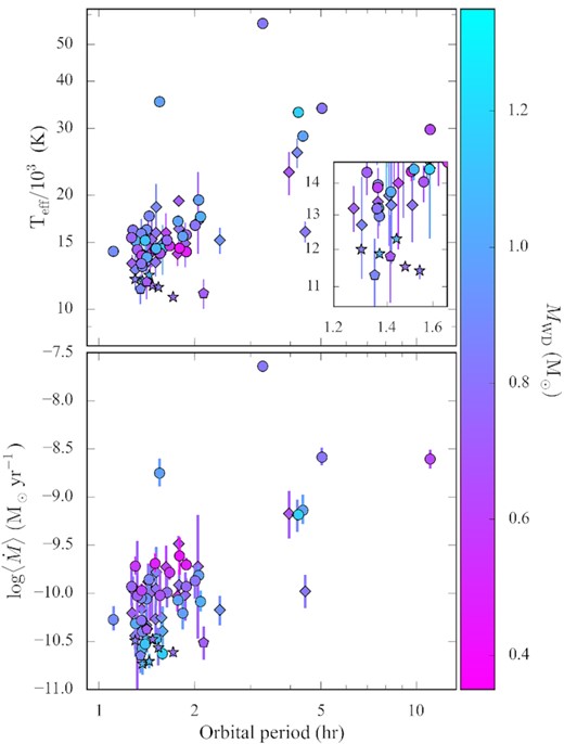
Effective temperatures (top) and mass accretion rates (bottom) as a function of the orbital period, for the systems in our HST sample (circles for pre-bounce and stars for period bounce CVs) and those from the literature (diamonds for pre-bounce and pentagons for period bounce CVs). The inset shows a closeup of the period bounce systems.
Two outliers clearly stand out: SDSS J153817.35+512338.0 (|$\rm{P_\mathrm{orb}} = 93.11\,$| min) and DW UMa (|$\rm{P_\mathrm{orb}} = 196.71\,$| min), which are both much hotter than the other CV white dwarfs at similar orbital periods. As already suggested by Pala et al. (2017), SDSS J153817.35+512338.0 could be a young CV which just formed at this orbital period and is undergoing a phase of high mass accretion rate that is expected to occur at the onset of the mass transfer (D’Antona, Mazzitelli & Ritter 1989). An alternative possibility is a CV that recently experienced a nova eruption and the white dwarf has not cooled down yet. DW UMa is a member of the nova-like CV subclass,10 which dominates the population of CVs in the 3−4 h period range. Possibly, also the high temperature and mass accretion rate of DW UMa, and those of nova-likes in general, could be related to their young ages if CVs are preferentially formed in the 3−4 h |$\rm{P_\mathrm{orb}}$| range (Townsley & Gänsicke 2009). This could be the case if the initial mass ratio distribution of main sequence binaries peaks towards equal masses (de Kool 1992). Alternatively, nova-likes could arise naturally from systems close to the regime of unstable mass transfer (Goliasch & Nelson 2015), where the mass of the donor star is similar to the white dwarf mass. These two outliers are not considered in the following discussion since their effective temperatures possibly reflect peculiar stages of their evolution.
Below the period gap, two branches are visible. One is composed of systems with |$\rm{T_\mathrm{eff}} \ge 12\, 500\,$| K, whose temperatures and mass accretion accretion rates decrease as the systems evolve towards the period minimum. The second branch consists of the period bounce CVs, which are evolving towards longer orbital periods and can be easily recognized as such thanks to their effective temperatures being |$\simeq 3000 \!-\! 4000\,$| K lower than those of the pre-bounce CVs at similar orbital periods (see the inset in the top panel of Fig. 12). We identify seven previously known period bouncers (EG Cnc, Patterson 2011; GD 552, Unda-Sanzana et al. 2008; SDSS J103533.02+055158.4, Littlefair et al. 2006; SDSS J150240.98+333423.9, McAllister et al. 2017; 1RXS J105010.8–140431, Patterson 2011; Pala et al. 2017, QZ Lib, Pala et al. 2018 and V455 And Patterson 2011) and two new period bounce CVs, SDSS J143544.02+233638.7 and CTCV J1300–3052. The fraction of period bouncers is thus |$(13 \pm 4)\,$| per cent, consistent with that derived by Pala et al. (2020) from the analysis of a volume-limited sample of CVs (|$7\!-\!14\,$| per cent).
We also noticed three additional weaker candidates (WZ Sge, SDSS J080434.20+510349.2 and SDSS J123813.73–033932.9), which are all known to host brown-dwarf companions (Howell, Harrison & Szkody 2004; Zharikov et al. 2013; Pala et al. 2019). However, these white dwarfs are slightly hotter (|$\rm{T_\mathrm{eff}} \simeq 13\, 000\,$| K) than other confirmed period bouncers and, since they are located right at the period minimum, it is difficult to asses whether they have already bounced back or not.
For the short period systems, we found that the white dwarf effective temperatures show a very weak dependence on the masses, i.e. systems hosting white dwarfs spanning a wide range in masses (|$0.4\!-\!1.2\, \mathrm{M_\odot }$|) all have very similar temperatures (left-hand panel in Fig. 13). From the statistical point of view, this is confirmed by the Pearson coefficient ρ = 0.07 and p-value = 0.62 of the distribution. In contrast, the mass accretion rates appear to be anticorrelated with the white dwarf mass. Note that, for a given |$\langle \dot{M} \rangle$|, |$\rm{T_\mathrm{eff}}$| increases as the layer of accreted material builds up to the next classical nova eruption (Townsley & Bildsten 2004). Below the period gap, the expected range of variation of |$\rm{T_\mathrm{eff}}$| is of the order of |$\pm 1000\,$|K and implies that the combination of |$\rm{T_\mathrm{eff}}$| and MWD via equation (6) does not provide a single value for |$\langle \dot{M} \rangle$|, but rather a range of possible mass accretion rates with a flat probability distribution. Nonetheless, this effect is not large enough (see e.g. fig. 10 from Townsley & Bildsten 2004) to explain the scatter observed in the left-hand panel of Fig. 13. In contrast, the |$\langle \dot{M} \rangle - M_\mathrm{WD}$| dependency directly descends from the white dwarf mass–radius relationship. Given that the quiescence luminosity is very weakly dependent on the white dwarf mass (equation 6), it follows that |$L \propto \langle \dot{M} \rangle \propto R_\mathrm{WD} ^{2} \rm{T_\mathrm{eff}} ^{4}$|. Therefore |$\langle \dot{M} \rangle \propto R_\mathrm{WD} ^{2}$|, since |$\rm{T_\mathrm{eff}}$| is observed to have no clear dependence on the mass. For comparison, this dependency is plotted as the solid black line in the left-hand panel in Fig. 13, which has been computed using the mass–radius relationship of Holberg & Bergeron (2006), Tremblay et al. (2011), and has been arbitrarily normalized so that |$\langle \dot{M} \rangle = 7\times 10^{-11}\, \mathrm{M_\odot } \mathrm{yr^{-1}}$| for |$M_\mathrm{WD} = 0.8\, \mathrm{M_\odot }$|.
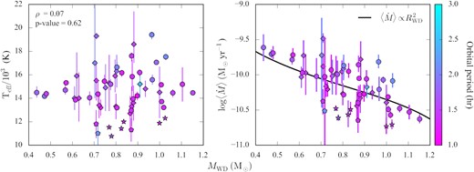
For systems at short orbital periods (|$\rm{P_\mathrm{orb}} \lt 3\,$| h), the white dwarf effective temperatures show no clear dependency on the white dwarf mass (left). Consequently, the relation between the mass accretion rates and the mass of the white dwarf (right) is dominated by the mass–radius relationship (|$\langle \dot{M} \rangle \propto R_\mathrm{WD} ^2$|, solid black line, arbitrarily normalized so that |$\langle \dot{M} \rangle = 7\times 10^{-11} \,\mathrm{M_\odot } \mathrm{yr^{-1}}$| for |$M_\mathrm{WD} = 0.8\, \mathrm{M_\odot }$|). The data are colour coded according to the orbital periods and the symbol convention is the same as in Fig. 12.
This behaviour differs significantly from the predictions of the classical models of CV evolution, which assume that, in this period range, angular momentum is mainly removed by gravitational wave radiation. This mechanism implies higher accretion rates (and hence higher effective temperatures) for larger white dwarf masses because the (i) the rate of gravitational wave radiation is directly proportional to the masses of the two stellar components in the system, and (ii) RWD is smaller for more massive white dwarf while the surface luminosity is not strongly dependent on MWD and thus |$\rm{T_\mathrm{eff}} \propto R_\mathrm{WD} ^{-2}$| (Townsley & Bildsten 2004). For comparison with this model, in the left-hand panels of Fig. 14, we show our results against various evolutionary tracks computed with MESAbinary (revision 15140) assuming magnetic wind braking and gravitational wave radiation above the period gap, and gravitational wave radiation only below the period gap, for different initial white dwarf masses. For completeness, these models also account for the loss of angular momentum associated with mass ejection following a classical nova eruption (assuming that all the accreted material is ejected), which is, however, negligible compared to magnetic wind braking and gravitational wave radiation. The models cover a much wider range in temperatures than the observations and predict a strong correlation between the white dwarf effective temperature and mass, with more massive CV white dwarfs being hotter than their less massive counterparts. They also imply lower accretion rates than observed and a direct correlation between the accretion rates and the white dwarf mass, i.e. CVs hosting more massive white dwarfs have higher accretion rates. Moreover, the evolutionary tracks underestimate the location of the period minimum and are not able to reproduce the observed temperatures of period bounce CVs. This is also the case for similar evolutionary models available in the literature (see e.g. fig. 3 from Howell, Nelson & Rappaport 2001 or fig. 2 from Goliasch & Nelson 2015), which in general predict that all systems, soon after the onset of mass transfer, will converge into a narrow track in the |$\langle \dot{M} \rangle\!-\!\rm{P_\mathrm{orb}}$| plane, with a very weak dependence on their masses.

Effective temperatures (top) and mass accretion rates (bottom) as a function of the orbital period, for the systems in our HST sample (circles for pre-bounce and stars for period bounce CVs) and those from the literature (diamonds for pre-bounce and pentagons for period bounce CVs). For a comparison with the models, we show the theoretically predicted values for the classical recipe for CV evolution (left-hand panels, see the text for more details) and for eCAML (right-hand panels, small dots), as computed by Belloni et al. (2020). Observations and theoretical values are colour coded according to the white dwarf mass. The mesa tracks have been computed assuming the following combination for the masses of the white dwarf and the donor (top to bottom): |$M_\mathrm{WD}=1.2\, \mathrm{M}_\odot$| and |$M_\mathrm{2}=0.8\, \mathrm{M}_\odot$|; |$M_\mathrm{WD}=1.0\, \mathrm{M}_\odot$| and |$M_\mathrm{2}=0.8\, \mathrm{M}_\odot$|; |$M_\mathrm{WD}=0.8\, \mathrm{M}_\odot$| and |$M_\mathrm{2}=0.6\, \mathrm{M}_\odot$|; |$M_\mathrm{WD}=0.6\, \mathrm{M}_\odot$| and |$M_\mathrm{2}=0.5\, \mathrm{M}_\odot$|; |$M_\mathrm{WD}=0.4\, \mathrm{M}_\odot$| and |$M_\mathrm{2}=0.3\, \mathrm{M}_\odot$|.
These theoretical results are in contrast with our findings, which suggest that the classical recipe of CV evolution needs to be revised in order to explain the absence of a clear dependency of the effective temperature on the white dwarf mass. The effective temperature is set by the secular mass accretion rate on to the white dwarf which, in turn, reflects the rate of angular momentum loss in the system. Therefore, our results suggest that the missing ingredient of the theoretical modelling causing low-mass CV white dwarfs to be hotter than predicted by the classical recipes (and to have similar effective temperature to their more massive counterparts, left-hand panel of Fig. 13) is an additional source of angular momentum loss which is more efficient the lower the mass of the white dwarf (right-hand panel of Fig. 13).
Such a dependency of the angular momentum loss rate on the white dwarf mass is the fundamental concept of the eCAML prescription developed by Schreiber et al. (2016) and Belloni et al. (2018, 2020) and already discussed in Section 1. This model includes an empirically mass-dependent additional source of angular momentum loss that better accounts for the observed dependency of the accretion rates on the white dwarf mass and better reproduces the observed temperatures and mass accretion rates (right-hand panels in Fig. 14) than the classical models. The enhanced angular momentum loss leads to a faster erosion of the donor star, causing the systems to bounce at longer orbital periods. Consequently, the period minimum predicted by eCAML is anticipated compared to the standard prediction and agrees better with the observations. Moreover, without requiring any additional fine-tuning, eCAML is also able to solve other disagreements that, for long time, have been found between the standard model of CV evolution and the observed properties of the CV population (such as their space density, and orbital period and mass distributions Schreiber et al. 2016; Belloni et al. 2020; Pala et al. 2020).
Despite the significant progress that is provided by the eCAML prescription, our observations provide reasons for improving this model in order to account for (i) the observed scatter in the parameters, (ii) the period bounce systems, for which the models predict a steep decrease in their effective temperatures that is not observed in data (which, instead, suggest the presence of enhanced angular momentum loss also in the post-bounce regime, as previously discussed also by Pala et al. 2017, 2020), and (iii) the presence of helium-core white dwarfs. The difference between the null fraction of helium white dwarfs predicted by eCAML and the observations is not as dramatic as in the case of the former estimates from more classical evolutionary models (see also Section 4.3). Our results suggest that some low mass systems can survive (at least for some time) in a semi-detached configuration, thus providing valuable observational constraints to further refine this model and thereby help to understand the physical mechanism that is driving the additional angular momentum loss.
Different authors have suggested that an additional source of angular momentum loss that is more efficient the lower the mass of the white dwarf could arise from friction between the binary and the shell of ejected material following a nova eruptions (Nelemans et al. 2016; Schreiber et al. 2016; Sparks & Sion 2021). To further investigate this possibility, our observational and theoretical understanding of classical novae and their impact on the secular evolution of CVs need to be improved.
Finally, additional issues are observed for systems above the period gap. The 3–4 h period range is mainly populated by the unexpectedly hot nova-likes CVs (which have already been discussed in the first part of this section) while, at |$\rm{P_\mathrm{orb}} \gtrsim 4\,$| h, CV white dwarfs are found to be systematically colder than predicted. This is a long-standing issue in our understanding of compact binary evolution (Knigge et al. 2011; Pala et al. 2017) and, as discussed in great detail by Townsley & Gänsicke (2009) and Belloni et al. (2020), could be related to either inaccurate modelling of magnetic wind braking (the dominant angular momentum loss mechanism driving the evolution of the systems in this period range) or incomplete understanding of the heating of the white dwarf as a consequence of the mass accretion process (for example, owing to the presence of long-term mass-transfer rate fluctuations associated with the secondary, to which long period CVs would be more susceptible than short-period systems, Knigge et al. 2011). However, the limited number of available measurements (eight) severely limits any conclusions we can draw in this period range and more observations are needed to increase the number of systems with accurate parameters above the period gap.
5 CONCLUSIONS
We analysed high quality HST ultraviolet spectra for 42 CVs. Making use of the astrometry delivered by the ESA Gaia space mission in its EDR3, we accurately measured the white dwarf effective temperatures and masses. We complemented this sample with an additional mass measurement for the white dwarf in AX For, obtained from its gravitational redshift. Our results are in good agreement with independent measurements obtained from analysis of the white dwarf eclipses and from radial velocity studies.
Combining our results with the effective temperatures and masses for 46 CV white dwarfs from the literature, we assembled the largest sample of systems with accurate white dwarf parameters. We derived an average white dwarf mass of |$\langle M_\mathrm{WD} \rangle = 0.81^{+0.16}_{-0.20}\, \mathrm{M_\odot }$|, in perfect agreement with former results, which allows us to definitively rule out any systematics affecting the masses derived from the analysis of eclipse light curves. In our mass distribution, we identify a tail extending towards low masses, consisting of five systems with |$M_\mathrm{WD} \lt 0.5\, \mathrm{M_\odot }$|. Such low masses are consistent with either He core or, possibly, hybrid CO/He core white dwarfs.
The white dwarf response to the mass accretion process and its capability to retain the accreted mass are of key interest in the context of Type Ia Supernova (SNe Ia) progenitors. If the mass transfer process can lead to the mass growth of the white dwarf, CVs could represent a possible channel for SN Ia explosions. By comparing the average mass of the white dwarfs in long (|$\rm{P_\mathrm{orb}} \gt 3\,$| h) and short (|$\rm{P_\mathrm{orb}} \lt 3\,$| h) period CVs, we do not find any evidence for a clear dependency on the white dwarf mass with the orbital period. However, additional measurements at long orbital periods are required to further constrain any correlation.
Thanks to the accurate parallaxes provided by Gaia, we have been able to measure both the white dwarf masses and temperatures. The combination of these parameters allows us to derive the secular mean of the mass accretion rates on to the white dwarf, which can be used to test and constrain the current models of CV evolution. For CVs at short orbital periods (|$\rm{P_\mathrm{orb}} \lt 3\,$| h), we show an anticorrelation between the mass accretion rates and the mass of the white dwarf, which implies the presence of an additional mechanism of angular momentum loss that is more efficient the lower the mass of the white dwarf. This finding is in very good agreement with the predictions of the recently proposed eCAML prescription. Including an empirically mass-dependent additional source of angular momentum loss, eCAML is able to explain the observed high average mass of CV white dwarfs and also to solve other disagreements between theory and observations, including the CV space density and orbital period distribution. The eCAML model provides an improved understanding of the observational properties of CVs and our results provide observational support for it. Some disagreement between eCAML and the observations still need to be addressed, like the observed scatter in the parameters and the presence of helium-core white dwarfs. Nonetheless, we highlight that the difference between the null fraction predicted by eCAML and the observations is not as dramatic as in the case of the former estimates from more classical evolutionary models. Our results suggest that some low-mass systems can survive (at least for some time) in a semi-detached configuration, thus providing valuable observational constraints to understand the physical mechanism that is driving the additional angular momentum loss.
Finally, an additional discrepancy between theory and observations is noticeable for the period bounce systems, for which the models predict a steep decrease in their |$\rm{T_\mathrm{eff}}$| and |$\langle \dot{M} \rangle$| that is not observed in data, which, instead, suggest the presence of enhanced angular momentum loss also in the post-bounce regime.
SUPPORTING INFORMATION
online_material.pdf
Please note: Oxford University Press is not responsible for the content or functionality of any supporting materials supplied by the authors. Any queries (other than missing material) should be directed to the corresponding author for the article.
ACKNOWLEDGEMENTS
This work has made use of data from the European Space Agency (ESA) mission Gaia (https://www.cosmos.esa.int/gaia), processed by the Gaia Data Processing and Analysis Consortium (DPAC, https://www.cosmos.esa.int/web/gaia/dpac/consortium). Funding for the DPAC has been provided by national institutions, in particular the institutions participating in the Gaia Multilateral Agreement.
The research leading to these results has received funding from the European Research Council under the European Union’s Seventh Framework Programme (FP/2007–2013) / ERC Grant Agreement n. 320964 (WDTracer).
The work presented in this article made large use of topcat and stilts Table/VOTable Processing Software (Taylor 2005).
BTG was supported by the UK Science and Technology Facilities Council (STFC) grant ST/P000495 andST/T000406/1. TRM acknowledges support from STFC grants ST/T000406/1 and from a Leverhulme Research Fellowship.
DB was supported by the grant #2017/14289-3, São Paulo Research Foundation (FAPESP) and ESO/Gobierno de Chile.
MRS acknowledges support from Fondecyt (grant 1181404) and ANID, – Millennium Science Initiative Program – NCN19_171.
PS acknowledges support from NSF grant AST-1514737 and NASA grant HST GO-15703.
DDM acknowledges support from the Italian Space Agency (ASI) and National Institute for Astrophysics (INAF) under agreements I/037/12/0 and 2017-14-H.0 and from INAF projects funded with Presidential Decrees N.43/2018 and N.70/2016.
DATA AVAILABILITY
All data underlying this article is publicly available from the relevant observatory archive or will be shared on reasonable request to the corresponding author.
Footnotes
It is worth mentioning that also the Far Ultraviolet Spectroscopic Explorer (FUSE) and the International Ultraviolet Explorer (IUE) provided a plethora of CV ultraviolet spectra. However, the wavelength range (|$\simeq 920 \!-\! 1180\,$| Å) of the FUSE observations is too limited for an accurate spectral fit with atmosphere models for white dwarfs with |$\rm{T_\mathrm{eff}} \lesssim 20\, 000\,$| K. This is because their spectra are characterized by a low-flux level due to the broad absorption lines from the higher orders of the Lyman series and, possibly, are complicated by heavy contamination from interstellar H2. In IUE, the 45-cm diameter mirror only allowed good signal-to-noise ratio observations of the brightest CVs.
Pala et al. (2017) reported that AX For went into outburst five days before the HST observations. The analysis of the ultraviolet data provides only a lower limit on the white dwarf mass. Nonetheless, we included this system in our sample since we measured its mass from additional optical phase-resolved observations.
The distance to the targets in our sample have also been computed from their Gaia EDR3 parallaxes by Bailer-Jones et al. (2021), with a method which also employs an exponentially decreasing volume density prior and a scale height calibrated against the stellar distribution at different Galactic latitudes. Nonetheless, we preferred to recompute the distances to our targets following the method described in Pala et al. (2020), since it employs a scale height that accounts for the age of the systems (as described in Pretorius et al. 2007) and is therefore more representative of the properties of the CV population.
See the document ‘Re-normalizing the astrometric chi-square in Gaia DR2’, which can be downloaded from: https://www.cosmos.esa.int/web/gaia/public-dpac-documents
A report on the wavelength shift can be found at https://www.eso.org/sci/facilities/paranal/instruments/xshooter/doc/XS_wlc_shift_150615.pdf
The evolution of CVs hosting magnetic white dwarfs is different compared to that of non-magnetic CVs, as there are evidence of the reduction of magnetic braking efficiency due to the coupling of the secondary and the white dwarf magnetic fields (Belloni et al. 2020). Our HST sample contains one strongly magnetised CV white dwarf (AM Her) which we do not include in the discussion.
Effective temperatures obtained during a low state are available for other two nova-like CVs, TT Ari (|$\rm{P_\mathrm{orb}} = 198.07$| min, |$\rm{T_\mathrm{eff}} =39\, 000$| K, Gänsicke et al. 1999) and MV Lyr (|$\rm{P_\mathrm{orb}} = 191.38\,$| min, |$\rm{T_\mathrm{eff}} =47\, 000$| K, Hoard et al. 2004). Similarly to DW UMa, both systems are much hotter than other CV white dwarfs at similar orbital periods. However, TT Ari and MV Lyr lack of an accurate mass measurement and therefore they have not been included in this analysis.
