


ABSTRACT
We present spectroscopic analysis of the luminous X-ray source Melnick 33Na (Mk 33Na, HSH95 16) in the Large Magellanic Cloud (LMC) 30 Doradus region (Tarantula Nebula), utilizing new time-series Very Large Telescope/Ultraviolet and Visual Echelle Spectrograph spectroscopy. We confirm Mk 33Na as a double-lined O-type spectroscopic binary with a mass ratio q = 0.63 ± 0.02, e = 0.33 ± 0.01, and orbital period of 18.3 ± 0.1 d, supporting the favoured period from X-ray observations obtained via the Tarantula – Revealed by X-rays survey. Disentangled spectra of each component provide spectral types of OC2.5 If* and O4 V for the primary and secondary, respectively. Unusually for an O supergiant the primary exhibits strong C iv 4658 emission and weak N v 4603-20, justifying the OC classification. Spectroscopic analysis favours extreme physical properties for the primary (Teff = 50 kK, log L/L⊙ = 6.15) with system components of M1 = 83 ± 19 M⊙ and M2 = 48 ± 11 M⊙ obtained from evolutionary models, which can be reconciled with results from our orbital analysis (e.g. M1sin 3i = 20.0 ± 1.2 M⊙) if the system inclination is ∼38° and it has an age of 0.9–1.6 Myr. This establishes Mk 33Na as one of the highest mass binary systems in the LMC, alongside other X-ray luminous early-type binaries Mk34 (WN5h+WN5h), R144 (WN5/6h+WN6/7h), and especially R139 (O6.5 Iafc + O6 Iaf).
1 INTRODUCTION
The mass of a star is its fundamental defining property, but direct measurements remain elusive with the exception of visual binaries or eclipsing spectroscopic binaries (Andersen 1991; Serenelli et al. 2021). Consequently mass estimates usually follow from spectroscopic results or comparison with evolutionary predictions. Uncertainties of evolutionary models increase with stellar mass (e.g. Martins & Palacios 2013) due to uncertainties in nuclear reaction rates, stellar structure, internal mixing processes, and mass-loss properties (Langer 2012), so stellar mass estimates of high-mass stars remain poorly constrained. Eclipsing double-lined spectroscopic binaries (SB2s) are the ideal gold standard calibrators to test single-star evolutionary models, because they permit accurate determinations of the dynamical mass, stellar parameters, and chemical abundances for both components. Most studies of such systems have focused on stars up to 15 M⊙ which only consider convective core overshooting and rotational mixing (e.g. Southworth, Maxted & Smalley 2004; Tkachenko et al. 2014; Pavlovski, Southworth & Tamajo 2018). Higgins & Vink (2019) also included the effect of mass-loss, which strips the stellar envelope and reveals CNO-processed material. They calibrated their grid of stellar models with the 40 + 34 M⊙ eclipsing massive supergiant binary HD 166734 (O7.5If + O9I(f)) using the results for this system from Mahy et al. (2017).
Despite the high binary frequency amongst massive stars (Sana et al. 2012, 2013) eclipsing systems are rare. Within the Milky Way, there are very few massive eclipsing binaries whose component masses exceed a few tens of solar masses, including NGC 3603 A1 with system components of 116 + 89 M⊙ (Schnurr et al. 2008), F2 in the Arches cluster with 82 + 60 M⊙ (Lohr et al. 2018), and WR20a with 71 + 69 M⊙ (Bonanos et al. 2004). Such systems are also scarce in the Magellanic Clouds, although a few massive systems have been identified via MACHO, OGLE, or targeted photometric surveys (e.g. Massey, Penny & Vukovich 2002; Ostrov & Lapasset 2003; Bonanos 2009). By way of example, as part of the TMBM (Almeida et al. 2017) follow-up to the VFTS survey of OB stars in the Tarantula Nebula (Evans et al. 2011), only four of ∼100 O-type binaries were identified as detached eclipsing binaries (Mahy et al. 2020).
SB2s are relatively common amongst massive stars and provide accurate orbital parameters, although the inclination must be inferred in order to derive the dynamical masses of the individual components. If the orbital solution is known, SB2 spectra can be disentangled and stellar parameters and chemical compositions obtained for the primary and secondary components. In the Large Magellanic Cloud (LMC) there are a few very massive SB2s, the majority of which are located in the Tarantula Nebula (Crowther 2019), including Melnick 34 whose primary component has been estimated to be 139 M⊙ (Tehrani et al. 2019), R144 with a primary mass of 74 M⊙ (Shenar et al. 2021), and R139 whose primary exceeds 69 M⊙ (Mahy et al. 2020). In principle, inclinations and in turn dynamical masses can be obtained for binaries lacking photometric eclipses via optical (e.g. Shenar et al. 2021) or X-ray light-curve modelling. Indeed, Melnick 34 (Pollock et al. 2018) was first established as a colliding-wind binary (CWB) via the Chandra X-ray imaging survey of the Tarantula Nebula, Tarantula – Revealed by X-rays (T-ReX, Townsley et al., in preparation; Broos & Townsley, in preparation).
Melnick 33Na (Mk 33Na) is located at a projected distance of ∼3.4 pc from the rich star cluster R136 in the Tarantula Nebula (Crowther & Dessart 1998; Massey & Hunter 1998). Melnick (1985) first identified ‘Mk 33N’ as an early O-type star (O4), with ‘Mk 33S’ ∼2 arcsec to the south-west (SW). Massey & Hunter (1998) refined its spectral type to O3 If* from Hubble Space Telescope (HST)/ Faint Object Spectrograph (FOS) spectroscopy (alias # 16 from Hunter et al. 1995) with ‘a’ added by Crowther & Dessart (1998) to distinguish it from ‘b’, an O6.5 V star (alias # 32 from Hunter et al. 1995) 1.2 arcsec away as shown in Fig. 1. Other aliases for Mk 33Na include # 1140 in Parker (1993), # 33 in Selman et al. (1999), and # 1943 in Castro et al. (2018).
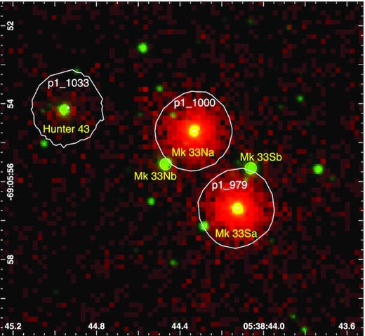
Two-colour composite image of Melnick 33 HST/WFC3 F555W (green; De Marchi et al. 2011) and Chandra ACIS (red; Townsley et al., in preparation) indicating the target of the current study Mk 33Na and its close visual companions Mk 33Nb (O6.5 V), Mk 33Sa (O3 III(f*); Massey et al. 2005), and Mk 33Sb (WC4 + OB; Smith, Shara & Moffat 1990). Mk 33Na and Mk 33Sa are bright X-ray sources, while Mk 33Nb and Mk 33Sb remain undetected in >2 Ms of Chandra data. The field of view is 8 × 8 arcsec (2 × 2 parsec at the distance of the LMC), with north up and east to the left. The rich star cluster R136 lies 3 parsec to the SW.
Shallow Chandra X-ray observations revealed Mk33 Na as a bright X-ray source (CX9 in Portegies Zwart, Pooley & Lewin 2002; # 133 in Townsley et al. 2006), with a similar X-ray luminosity (LX) to R139, suggesting the presence of a CWB. Deep X-ray imaging via the T-ReX survey (Townsley et al., in preparation) confirmed Mk33Na as a bright X-ray source (Fig. 1) corresponding to an attenuated X-ray luminosity of 2.8 × 1033 erg s−1 at the distance of the LMC (Crowther et al., in preparation). On the basis of its Kuiper statistic, a variant of the Kolmogorov–Smirnov test (Paltani 2004) shown in Fig. 2, Broos & Townsley (in preparation) identified significant X-ray variability suggesting a potential period of 18.3 d for Mk 33Na most likely due to orbital modulation in a binary system. Fig. 1 shows that Mk33Sa is similarly bright in X-rays suggestive perhaps of another binary, although it is less variable than its neighbour.
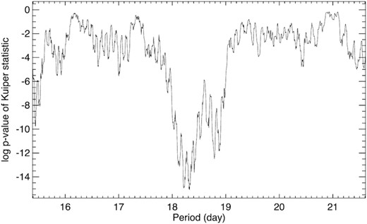
A period search for Mk 33Na from X-ray observations with the Chandra T-ReX survey of the Tarantula Nebula (Townsley et al., in preparation; Broos & Townsley, in preparation), favouring a period of ∼18.3 d from the observed Kuiper statistic (Paltani 2004).
Here, we undertake an analysis of Very Large Telescope (VLT)/Ultraviolet and Visual Echelle Spectrograph (UVES) time-series spectroscopy of Mk 33Na motivated by the T-ReX observations, confirm that it is an SB2 with a period of ∼18.3 d, estimate its physical and wind properties, and reveal that it comprises a CWB with a high LX/Lbol = 1.2 × 10⁻⁶ (Crowther et al., in preparation). In Section 2, we present our orbital analysis of new VLT/UVES spectroscopy and X-ray variability of Mk 33Na. Section 3 presents the spectral types of each disentangled component plus a spectroscopic analysis from which physical, wind, and chemical properties are obtained. Stellar masses, ages, and orbital inclination are presented in Section 4. We discuss our results in the context of other massive binaries in the LMC in Section 5 and brief conclusions are drawn in Section 6.
2 OBSERVATIONS
Using optical multi-epoch observations (Section 2.1) we determine the radial velocity (RV) variations of both components of the Mk 33Na system (Section 2.2). The orbital parameters are calculated in Section 2.3 and the X-ray observations are presented in Section 2.4.
2.1 Optical spectroscopy
To determine the orbital parameters we spectroscopically followed up Mk 33Na (RA 05:38:44.34, Dec -69:05:54.6, J2015.5, and Gaia DR2; Gaia Collaboration 2018) with the UVES (Dekker et al. 2000) mounted at the VLT in Paranal, Chile. 15 epochs of VLT/UVES spectra were obtained in service mode over a period of 17 d in 2020 October (Program ID 106.21MH.001 aka 5106.D-0835(A), PI: Bestenlehner). The observations were initially planned to sample the orbital period over 2.5 months with preferences on dates where service mode was available. Each epoch or orbital phase could be potentially observed on 2 or 3 dates. According to the Phase 2 guidelines one to two epochs per orbital phase were scheduled on days when service mode was not available. In the unlikely event that all epochs are obtained in one go including dates where service mode was not available, possible coverage periods were between 17 and 19 d.
Due to Covid-19, regular observations with the VLT paused earlier in 2020. VLT/UVES was one of the first instruments to be brought back in operation for service mode only, from the beginning of 2020 October. All 15 epochs were obtained on the nights of October 8–25 or in Modified Julian Date (MJD) from 59131.25 to 59148.18 d, even though some nights were originally flagged as no service mode available, as indicated in the observations log (Table 1). The slit was placed north to south with a slight angle avoiding stars directly in the slit (Fig. 1). Observations were taken in Dichroic 2 mode with central wavelengths of 437 and 760 nm, providing spectral ranges of 3730–4990 Å (blue-arm, EEV 2k×4k detector), 5670–7570 Å (lower red-arm, EEV 2k×4k detector), and 7670–9450 Å (upper red-arm, MIT/LL 2k×4k detector) with an integration time of 593 s. A 0.8 arcsec slit was used for all epochs with a spectral resolution between 50 000 and 60 000. A signal-to-noise ratio (S/N) between 30 and 50 was achieved for the blue- and lower red-arm.
Observing log of VLT/UVES spectroscopy of Mk 33Na and measured RVs for the primary OC2.5 If* and secondary O4 V components.
| ut date | sec z | DIMM | MJD | N iv 4058 | C iv 5801 | He ii 4542 | Hη | He ii 4542 | Hη |
|---|---|---|---|---|---|---|---|---|---|
| arcsec | Primary | Primary | Primary | Primary | Secondary | Secondary | |||
| 2020 Oct 09 | 1.62 | 0.71 | 59131.25 | |$175.4^{+5.9 }_{-6.1 }$| | 199.1 ± 4.5 | 203.7 ± 9.4 | |$210.4^{+11.6}_{-12.6}$| | |$318.3^{+11.9}_{-12.0}$| | |$330.3^{+25.4}_{-22.3}$| |
| 2020 Oct 10 | 1.61 | 0.67 | 59132.25 | 233.4 ± 6.9 | |$225.0^{+4.6 }_{-4.7 }$| | 238.6 ± 8.4 | |$219.8^{+12.5}_{-13.1}$| | 317.3 ± 10.8 | |$382.0^{+21.2}_{-19.1}$| |
| 2020 Oct 11 | 1.60 | 0.49 | 59133.25 | |$241.8^{+5.8 }_{-6.3 }$| | |$252.6^{+6.5 }_{-6.2 }$| | 251.7 ± 8.9 | |$257.2^{+11.9}_{-12.2}$| | |$269.4^{+10.9}_{-10.8}$| | |$283.9^{+28.1}_{-27.1}$| |
| 2020 Oct 12 | 1.78 | 0.80 | 59134.21 | |$261.7^{+9.9 }_{-8.3 }$| | |$275.1^{+5.3 }_{-5.2 }$| | |$255.9^{+8.6}_{-8.5}$| | |$249.7^{+10.8}_{-10.9}$| | 266.6 ± 9.7 | |$210.9^{+26.8}_{-28.5}$| |
| 2020 Oct 14 | 1.97 | 0.82 | 59136.17 | |$290.8^{+9.2 }_{-10.8}$| | |$315.5^{+6.0 }_{-5.8 }$| | 293.4 ± 9.0 | |$279.1^{+15.2}_{-14.7}$| | |$192.9^{+13.7}_{-14.2}$| | |$196.1^{+26.4}_{-30.4}$| |
| 2020 Oct 15 | 1.79 | 1.07 | 59137.20 | |$299.3^{+12.9}_{-15.5}$| | |$330.6^{+7.5 }_{-7.1 }$| | 302.4 ± 11.1 | |$316.5^{+14.6}_{-13.7}$| | |$180.4^{+15.1}_{-15.5}$| | |$133.4^{+21.2}_{-24.1}$| |
| 2020 Oct 16 | 1.84 | 0.59 | 59138.19 | 317.3 ± 6.5 | |$335.7^{+5.9 }_{-5.8 }$| | 329.0 ± 9.1 | 288.9 ± 13.2 | 157.6 ± 10.6 | |$166.7^{+23.8}_{-25.5}$| |
| 2020 Oct 17 | 1.58 | 0.54 | 59139.24 | |$357.7^{+8.6 }_{-8.1 }$| | |$342.1^{+4.4 }_{-4.2 }$| | 346.8 ± 7.8 | |$314.4^{+9.3 }_{-8.9 }$| | 152.4 ± 8.4 | |$135.6^{+15.1}_{-16.0}$| |
| 2020 Oct 19 | 1.51 | 0.58 | 59141.26 | |$359.9^{+8.5 }_{-8.3 }$| | |$352.0^{+7.6 }_{-7.0 }$| | 336.1 ± 8.4 | |$327.2^{+10.2}_{-9.5 }$| | |$155.3^{+10.9}_{-10.7}$| | |$111.9^{+16.7}_{-18.0}$| |
| 2020 Oct 20 | 1.68 | 1.26 | 59142.21 | |$327.6^{+9.7 }_{-8.9 }$| | |$329.4^{+11.6}_{-12.1}$| | 305.2 ± 10.0 | |$316.6^{+15.2}_{-14.1}$| | |$179.8^{+13.6}_{-13.7}$| | |$80.8 ^{+33.9}_{-30.0}$| |
| 2020 Oct 21 | 1.67 | 0.47 | 59143.21 | |$316.1^{+5.6 }_{-5.4 }$| | |$314.0^{+5.3 }_{-5.4 }$| | |$297.8^{+8.4}_{-8.3}$| | |$304.4^{+11.3}_{-10.9}$| | |$201.6^{+9.6 }_{-9.8 }$| | |$161.9^{+21.3}_{-22.8}$| |
| 2020 Oct 22 | 1.83 | 0.71 | 59144.17 | |$263.5^{+7.9 }_{-7.3 }$| | |$249.4^{+5.7 }_{-5.6 }$| | |$255.1^{+8.8}_{-8.7}$| | |$262.4^{+14.4}_{-14.0}$| | |$272.4^{+10.7}_{-10.6}$| | |$276.7^{+39.8}_{-40.4}$| |
| 2020 Oct 24 | 1.72 | 0.62 | 59146.19 | |$129.4^{+7.0 }_{-6.8 }$| | |$135.9^{+6.2 }_{-6.1 }$| | 169.9 ± 8.2 | |$139.4^{+8.3 }_{-8.7 }$| | |$432.9^{+10.8}_{-11.0}$| | 520.2 ± 14.8 |
| 2020 Oct 25 | 1.41 | 0.96 | 59147.31 | |$126.6^{+7.3 }_{-6.6 }$| | |$140.3^{+5.2 }_{-5.0 }$| | |$148.5^{+8.4}_{-8.3}$| | |$146.0^{+8.6 }_{-9.0 }$| | |$494.9^{+9.5 }_{-12.8}$| | |$474.0^{+18.6}_{-19.2}$| |
| 2020 Oct 26 | 1.74 | 0.63 | 59148.18 | |$146.3^{+5.9 }_{-5.8 }$| | |$159.1^{+5.5 }_{-5.2 }$| | 160.8 ± 8.3 | |$174.4^{+17.2}_{-18.4}$| | 416.1 ± 16.2 | |$455.8^{+26.6}_{-28.0}$| |
For the data reduction, we used the European Southern Observatory Reflex pipeline (Freudling et al. 2013) with standard calibration data for service mode. Mk 33Na is located in a crowded region within the Tarantula nebula (Fig. 1). The default pipeline setting for flux-calibrated spectra took the entire slit into account. Even though we placed the slit in a way that minimized contamination from nearby sources, some of the spectra were still contaminated owing to high airmass (up to 2.0) and variable seeing conditions (DIMM1 0.5–1.3 arcsec). The WC star Mk33Sb was the most prominent source which affected He ii 4686 and the C iv 5801/5812 spectral lines (Fig. 1). Therefore, we chose the 2D slit extraction and co-added the regions which were the least contaminated by nearby sources. However, this led to a reduction in the S/N of the extracted spectra (between 25 and 35 for the blue- and lower red-arm, respectively).
In the final step, we applied to each epoch the barycentric correction to the wavelength array. To bring the wavelength array of the individual epoch to the same scale we used the interstellar band Ca ii 3934 for the blue-arm and Na i 5890 for the lower red-arm. As a reference value, we chose the average RV of the interstellar lines.
Spectra for each epoch are shown in the supplementary online material.
2.2 Radial velocities
Visual inspection showed that N iv 4058 and C iv 5801 hardly show any signatures of the secondary star. With the stellar atmosphere and radiative transfer code cmfgen (Hillier & Miller 1998), we computed a synthetic reference spectrum based on estimated stellar parameters from our spectral classification (Section 3.2). Using the synthetic spectrum, we performed χ2-minimization analyses to derive the RVs for N iv 4058 and C iv 5801.
The observation taken on October 25 (MJD = 59147.3122 d) revealed the largest separation of the He ii 4542 lines of the primary and secondary (Fig. S2, supplementary online material). This epoch was used to estimate the optical flux ratio of ∼0.25 for the individual components by scaling the templates of the primary and secondary by a factor of 0.8 and 0.2 to match the He ii line strength. According to the spectral classification, we chose a template for the secondary with an effective temperature of 45 000 K. As an initial RV guess for the primary we used the average of the N iv 4058 and C iv 5801 RV measurements for each epoch. Subsequently, we performed an iterative χ2-minimization analysis of He ii 4542 and Hη by alternately co-adding and shifting the template spectra of the primary and secondary until convergence. The nebular emission was clipped in the case of Hη. Lower excitation levels of the Balmer series showed too strong nebular lines and it was not possible to derive RV for all observations. The results are given in Table 1.
In Fig. 3, we visualize our RV measurements. It clearly shows the antiphase between the primary and secondary of the Mk 33Na system. The uncertainties of the RV measurements are larger for the secondary and in particular for Hη.
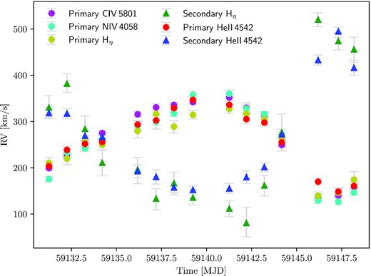
RV measurements versus MJD for the primary OC2.5 If* and secondary O4 V components.
2.3 Orbit fitting and orbital parameters
To determine the Keplerian orbital parameters, we used the Markov Chain Monte Carlo (MCMC) fitting routine developed, utilized and described in Tehrani et al. (2019). As input prior for the period, we used a uniform distribution of 18 ± 2 d according to the X-ray period from Fig. 2. A flat, uninformative prior was adopted for the other parameters. The MCMC fitting was performed using the uncertainties weighted averaged RV measurements from Table 3 for the primary and secondary. The routine delivers a full set of Keplerian orbital parameters: semi-amplitudes of the velocities of the primary (K1) and secondary star (K2), system velocity γ, eccentricity e, longitude of periastron ω, orbital period P, and time of periastron T0.
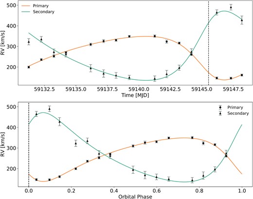
MCMC fit to determine the Keplerian orbital parameters of the Mk 33Na system. Solution for the primary and secondary are shown by the solid-orange and cyan-green lines. Black dots and triangle are the uncertainties weighted averaged RV measurements from Table 1 for the primary and secondary, respectively.
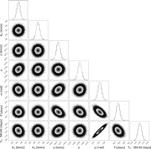
Corner plot showing posterior probabilities for the MCMC fit solution, where K1 and K2 are the semi-amplitudes of the velocities for the primary and secondary, respectively, γ is the systemic velocity, e is the eccentricity, ω is the longitude of the periastron, P is the orbital period, and T0 is the time of periastron.
All orbital parameters and minimum masses including uncertainties are given in Table 2.
Keplerian orbital parameters with 1σ uncertainties derived using the MCMC methods of Tehrani et al. (2019).
| Parameter | Unit | MCMC |
|---|---|---|
| K1 | km s−1 | 105.6 ± 1.5 |
| K2 | km s−1 | 168.2 ± 3.8 |
| γ | km s−1 | 266.5 ± 1.0 |
| e | 0.334 ± 0.010 | |
| ω | ° | 131.19 ± 2.86 |
| P | d | 18.319 ± 0.139 |
| T0 | MJD | 59145.53 ± 0.12 |
| Morb, 1sin 3i | M⊙ | 20.04 ± 1.23 |
| Morb,2sin 3i | M⊙ | 12.58 ± 0.85 |
| q | 0.628 ± 0.016 |
2.4 X-ray light curve
The 2 Ms Chandra Visionary Program T-ReX was executed over 630 d between 2014 May 3 and 2016 Jan 22 using the ACIS instrument (16.9 × 16.9 arcmin field of view) centred on R136a, the central star at the heart of the Tarantula Nebula cluster (Townsley et al.; in preparation). Here, we confirm the 18.3 d orbital period of Mk 33Na from UVES, supporting the X-ray results from the Kuiper statistic (Fig. 2) from the T-ReX data set (Broos & Townsley, in preparation). We present its X-ray light curve folded on the best-fitting optical RV period in Figs 6 and 7. The T-ReX campaign itself covered 34 orbital cycles suggesting a high degree of reproducibility for an X-ray source of mean count rate close to 1 count per ks. This conclusion is reinforced by the three relatively bright measurements taken close to an implied periastron about a decade and 165 orbital cycles earlier in 2006 January. The X-ray source list and source properties from the 2006 Chandra data on 30 Doradus were published in Townsley et al. (2014).
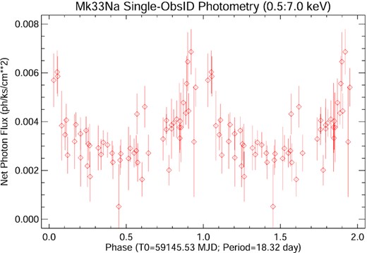
X-ray light curve of Mk 33Na folded on a period of 18.32 d about the periastron passage.
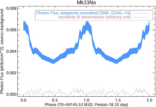
The phases of individual events are adaptively smoothed. The thickness of the blue ribbon represents the uncertainty of the flux estimate at that phase.
At first sight, Figs 6 and 7 appear consistent with the luminosity variations expected from a CWB system in which the X-ray cooling time exceeds the flow time out of the system leading to luminosity inversely proportional to the binary separation (e.g. Stevens, Blondin & Pollock 1992). However, the shape of the observed X-ray spectrum varies with phase as shown in Fig. 8. The rise in flux in the approach to periastron is mostly due to soft X-rays near 1 keV. Spectral analysis performed in four broad phase bins reveals that the data are consistent with a model in which a separation-dependent luminosity is further modulated by a phase-dependent absorbing column density, where NH/1022 = 1.5, 1.9, 2.1, and 1.7 cm−2 in phase bins -0.1:0.1, 0.1:0.3, 0.3:0.7, and 0.7:0.9 (Fig. 8).
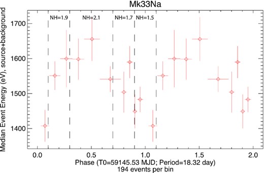
Folded median X-ray energy divided into 10 phase bins. Dashed vertical lines indicate four broad phase bins including the absorption column density (NH/1022, see text). The spectrum is softer near periastron as the binary-separation dependent luminosity is modulated by phase-dependent absorption.
Although other models can fit the data, this variable-absorber model offers a simple interpretation. The lowest absorbing column (maximum count rate) occurs when the shocked X-ray emission occurring in the space between the stars is viewed through the weaker wind of the secondary O4V star which passes in front across the line of sight 1.4 d before periastron, according to the orbital elements in Table 2. High reddening shows that the interstellar medium accounts for much of the observed X-ray absorption. The time-averaged X-ray luminosity of Mk 33Na is log LX = 33.95 ± 0.05 erg s−1 (Crowther et al., in preparation), a value more typical of binary systems than the lower intrinsic luminosities of single stars.
3 SPECTRAL TYPE AND SPECTROSCOPIC ANALYSIS
Before we determine the spectral types (Section 3.2) and perform the spectroscopic analysis (Section 3.5), we disentangled the spectra into primary and secondary components (Section 3.1). Line broadening and line-profile variations are described in Sections 3.3 and 3.4. The section concludes with Section 3.6 where we obtain reddening parameters and luminosities for primary and secondary star.
3.1 Disentangling
For an accurate spectral classification and reliable spectroscopic analysis, we disentangled the spectra into primary and secondary components. Individual components exhibit large RV variations which are enhanced by their antiphase (Fig. 3) making disentanglement relatively straightforward.
Based on the orbital solution from Section 2.3, we calculate more precise RVs for each epoch of the primary and secondary than measured in Section 2.2. In the first step, we shifted the epochs to the rest frame of the primary according to its RV. Co-adding and averaging the spectra would have included signatures of the secondary and for example cosmics which are not removed by 2D slit extraction (Section 2.1). Therefore, we calculated a median spectrum which should largely remove the secondary component. The difference between the both methods is shown in Fig. B1. To obtain the spectrum for the secondary, we applied the RV shift for each epoch to the primary median spectrum from the first step and divided the epoch by the primary spectrum (Fig. B2). Then, we shifted the epochs to the rest frame of the secondary and calculated the median spectrum of the secondary.
For an improved disentangling, we applied the same methodology for the primary by dividing all epochs by the secondary median spectrum before calculating the median spectrum of the primary. Those steps were repeated until no changes to the previous iteration were observed. The spectra of Mk 33Na1 and Mk 33Na2 are rescaled according to their flux ratio (Section 3.6).
A similar methodology was applied to remove the broad C iv 5801-12 emission caused by the WC4 star Mk33Sb (Figs 1 and B3). The disentangled spectra are shown in Figs 11 and 12. A detailed description of the spectra disentangling methodology is given in Appendix B.
3.2 Spectral type
Spectral types for the unresolved source Mk 33N from the literature include O4 from Melnick (1985), with spatial crowding hindering further progress until Massey & Hunter (1998) utilized HST/FOS to obtain spectra of Mk 33Na and b, from which classifications of O3 If* and O6.5 V, respectively, were obtained. From classification of our UVES spectroscopy, the criteria of Sota et al. (2011) were followed and verified with the spectral templates from Walborn et al. (2014). The most unusual feature of Mk 33Na is the clear presence of C iv 4658 and weakness of N v 4603-20 plus the strength of the C iv 5801-12 doublet in emission suggestive of an OC star for the primary component. The line ratio of the nitrogen lines is similar to VFTS 169 (O2.5 V(n)((f*)), but with a much stronger stellar wind as seen in the emission line strength of He ii 4686 and Hα which exceed the line strength of VFTS 016 (O2 III-If*, Fig. 9). VFTS 016 and Mk33Na1 have similar C iv 4658 line strength, but the nitrogen lines are stronger in VFTS 016 while weaker in the Mk 33Na1 spectrum (C iv 4658 > N v 4603–20). The carbon abundances (ϵC = log (C/H) + 12 = 7.82) of VFTS 016 and Mk33Na1 are comparable, but the nitrogen abundance (ϵN = log (C/H) + 12 = 7.76) of VFTS 016 is higher by ∼0.5 dex (Table 3; Evans et al. 2010). Therefore, we classified Mk 33Na1 as OC2.5 If*.
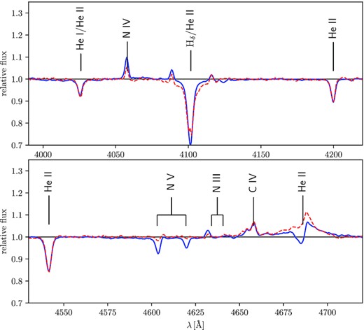
Spectral comparison of Mk 33Na1 (red-dashed line) with VFTS 016 (blue-solid line; Evans et al. 2010). C iv 4658 has a similar line strength in both stars, but the nitrogen lines are much weaker for Mk 33Na1⇒ OC2.5 If*.
Stellar parameters obtained from the spectroscopic analysis. Masses under the assumption of chemically homogeneous evolution (Mhom) are derived with the mass–luminosity relation by Gräfener et al. (2011). Most probable stellar parameters derived with BONNSAI (Schneider et al. 2014) based on stellar evolutionary models by Brott et al. (2011) and Köhler et al. (2015).
| Spectroscopic analysis | ||||||||||
|---|---|---|---|---|---|---|---|---|---|---|
| SpT | log L/L⊙ | Teff | Reff | log g | |$\log \dot{M}/\sqrt{f_{\rm V}}$| | ϵC | ϵN | Mhom | Msp | |
| K | R⊙ | cm s−2 | M⊙ yr−1 | log (C/H) + 12 | log (N/H) + 12 | M⊙ | M⊙ | |||
| Primary | OC2.5 If* | 6.15 ± 0.18 | |$50\, 000\pm 2500$| | 15.8 ± 2.1 | 4.0 ± 0.1 | –5.6 to –5.2 ± 0.2 | 7.7 ± 0.3 | 7.2 ± 0.3 | 106 | |$90^{+25}_{-18}$| |
| Secondary | O4 V | 5.78 ± 0.18 | |$45\, 000\pm 2500$| | 12.8 ± 1.7 | –a | –6.5b | – | – | 66 | – |
| Recovered stellar parameters by BONNSAI | ||||||||||
| SpT | log L/L⊙ | Teff | Reff | log g | Age | ϵC | ϵN | Mevo | Mevo, ini | |
| K | R⊙ | cm s−2 | Myr | M⊙ | M⊙ | |||||
| Primary | OC2.5 If* | 6.08 ± 0.14 | |$50\, 700^{+2500}_{-2200}$| | |$13.9^{+2.5}_{-2.0}$| | |$4.15^{+0.01}_{-0.17}$| | 0.9 ± 0.6 | 7.75c | 6.9c | 83 ± 19 | |$84^{+21}_{-19}$| |
| Secondary | O4 V | |$5.66^{+0.17}_{-0.19}$| | |$45\, 800^{+2800}_{-2700}$| | |$10.1^{+2.5}_{-2.0}$| | |$4.17^{+0.05}_{-0.21}$| | |$1.6^{+0.7}_{-1.3}$| | 7.75c | 6.9c | 48 ± 11 | |$47^{+13}_{-9}$| |
Note.
log g could not be derived, because the wings of the Balmer lines are in emission.
Approximate upper limit for the mass-loss rate.
The probability distribution function shows a wide spread of possible composition, but the most probable value is the initial chemical composition for the LMC (Brott et al. 2011).
The spectral type of the secondary (Mk 33Na2) is more difficult to determine. The absence of strong signatures of carbon and nitrogen lines is indicative for dwarfs with a relatively weak stellar wind. Based on the spectral types by Walborn et al. (2014), we noticed that VFTS 797 (O3.5 V((n))((fc))) shows similar spectral properties such as weak C, N, and He i 4471 lines and relatively strong He ii 4542 absorption line. N iv 4058 is not or hardly visible in the spectrum and there might be a hint of N iii 4634-41 and C iii 4650. We concluded that the spectral type of Mk 33Na2 is approximately O4 V.
3.3 Line broadening
If the binary system is tidally locked, the mean rotational velocity is |$2\pi R_{\rm eff}/P$| based on stellar radius and period of the system (Tables 2 and 3). In an eccentric orbit, the projected rotational velocity (|$v \sin i$|) should vary throughout the orbit and lower or equal to the mean rotational velocity, e.g. ≲ 50 km s−1 for the Mk33Na1. We used IACOB-BROAD (Simón-Díaz & Herrero 2014) to derive |$v \sin i$| and macro-turbulent velocity (|$v _{\rm mac}$|). IACOB-BROAD is an interactive analysis tool that combines Fourier transformation (FT) and goodness-of-fit methods. The code is publicly available and is written in the interactive data language.
We were only able to derive the line broadening for the primary based on the C iv 5801 line. Unfortunately, we were unable to employ metal lines in absorption to determine the line broadening which would provide more accurate measurements. We inferred |$v \sin i$| using the first minimum of the FT. The macro-turbulent velocity was determined based on the goodness of fit while |$v \sin i$| was set to the FT value. The measurements are listed in the Appendix (Table A1).
Fig. 10 shows |$v \sin i$| and |$v _{\rm mac}$| as a function of phase. For reference, the RV variations for the primary are included as well. Shortly after periastron, both broadening velocities drop below 60 km s−1. With the exception of a couple of outliers the average for |$v \sin i$| and |$v _{\rm mac}$| lies around 95 km s−1. Averaged |$v \sin i = 75.5\pm 0.6$| km s−1 and |$v _{\rm mac} = 110.3\pm 4.1$| km s−1 based on the measurements of N iv and C iv 5801-12 (Table A1). The stellar spectra of the primary show large line profile variations (LPVs) including the C iv 5801-12 doublet (Section 3.4). The outliers could be due to the dynamics within the stellar atmosphere and wind. However, we can conclude that the primary is not tidally locked.
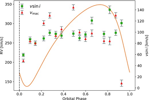
Projected rotational and macro-turbulent velocity of Mk 33Na1 as a function of orbital phase. The fit to the RV measurements (solid-orange line) is shown for reference.
For the secondary we were only able to measure |$v \sin i \approx 125$| km s−1 and |$v _{\rm mac}\approx 10$| km s−1 at the orbital phase ∼0.1 using He ii 4542. The He ii line is also broadened by the Stark effect and could lead to an overestimation of |$v \sin i$| and |$v _{\rm mac}$|. The |$v \sin i \approx 125$| km s−1 can be considered as an upper limit for the secondary. |$v \sin i$| and |$v _{\rm mac}$| based on the median spectrum is around 78 and 56 km s−1 for the C iv 5812 line (Table A1).
3.4 Line profile variations
Line profiles of some lines varied significantly throughout the orbit, e.g. He ii 4686, N iv 4058, and wings of Balmer lines. Shortly after periastron, He ii 4686 is weakest and N iv 4058 has nearly disappeared as well. At phase ∼0.1 the line strength suddenly increases and settles down again after 1 d. This could be an outburst of material, but N iv 4058 is hardly affected. The emission line strength increases until apastron at orbital phase 0.5 and decreases again with some variation towards periastron (Fig. A1).
There are noticeable variations in the wings of the absorption lines Hβ, Hγ, He ii 4200, and 4542 with filling in of an emission line component. As seen in Fig. 12 those features seem to belong to the secondary. Either the mass-loss rate varies significantly or those LPVs are caused by the stellar wind and ionizing flux of the primary star. However, the C iv 5801-12 doublet is very sensitive to the mass-loss rate and a small increase would turn the lines from absorption into emission.
A future study will try to understand the nature and physical processes of those variations including the X-ray variability (Section 2.4).
3.5 Spectroscopic analysis
The spectra were analysed with the spherical, non-local thermodynamic equilibrium stellar atmosphere and radiative transfer code CMFGEN (Hillier & Miller 1998). We used the grid of stellar atmospheres from Bestenlehner et al. (2014) to roughly estimate the stellar parameters. Based on the initial guesses, we computed a grid with an extended atomic model by varying the effective temperature Teff defined at an optical depth τ = 2/3, surface gravity log g, mass-loss rate |$\dot{M}$|, and chemical abundances of carbon and nitrogen. The terminal velocity (|$v _{\infty }$|) could only be derived for Mk 33Na1 based on the line width of He ii 4686 and Hα (|$v _{\infty } \sim\ 2200$| km s−1). The wind volume filling factor (fv) was set to 0.1 and |$v _{\rm mic}$| was set to 10 km s−1. The grid of stellar atmospheres contains the following element ions: H i, He i–ii, C ii–v, N ii–v, O ii–vi, Ne ii–v, Mg ii–iv, Ca iii–v, Si ii–vi, P iii–v, S iii–vi, Fe iii–vii, and Ni iii–vi.
We were only able to confidently derive stellar parameters for the primary. The effective temperature is based on the presence of C iv 4658 and the weakness of N v 4604-20 relative to N iv 4058. The surface gravity is derived from wings of Hγ − ϵ. The mass-loss rate is determined from the emission line strength of He ii 4686 which varies throughout the orbit. Hα was strongly contaminated by nebular lines and was not suitable. Due to CN cycle, the C abundance decreases and N increases during the main-sequence lifetime. However, the primary is still carbon-rich close to the LMC baseline of (ϵC − ϵN)LMC = 0.85 dex (Brott et al. 2011), with ϵC − ϵN = (ϵC − ϵN)LMC − 0.35 ± 0.4 dex, suggesting a young age for the binary system of less than ∼1 Myr.
The determination of stellar parameters for the secondary is less straightforward because of the emission line components in the wings of the Balmer and helium lines. As the log g is derived from the broadening of the wings of the Balmer lines, we were unable to determine the surface gravity for the secondary. The absence or the difficult identification of N iii 4634-41, N iv 4058, N v 4604-20, C iii 4650, the absorption of C iv 5801-12 and the presence of He i 4471 suggest a |$T_{\rm eff} = 45\, 000\pm 2500$| K for the secondary. C iv 5801-12 turns from absorption into emission if the mass-loss rate is increased. Other lines are hardly affected and we are only able to determine an upper mass-loss rate limit of |$\log \dot{M} [\mathrm{M}_{\odot }\,\mathrm{yr}^{-1}] \lt -6.5$|.
Physical, wind, and chemical properties of Mk 33Na are provided in Table 3 with corresponding spectroscopic fits of the disentangled spectra in Figs 11 and 12. Spectroscopic fits for each epoch are provided in the supplementary online material. The only previous spectroscopic analysis of the system was undertaken by Castro et al. (2021) who analysed He i 4921 and He ii 5411 lines of a large sample of 30 Doradus stars using VLT/Multi Unit Spectroscopic Explorer (MUSE) spectroscopy (CCE18, Castro et al. 2018) using a grid of FASTWIND models to obtain Teff = 36 kK and log L/L⊙ = 5.93, |$v \sin i$| = 170 km s−1 for Mk 33Na (= CCE18 1943), and an approximate spectral type of ‘O5’.
3.6 Stellar luminosities
Bolometric luminosities (L) of both components are derived by matching optical and near-infrared (near-IR) photometric data with the combined theoretical spectral energy distribution (SED). We employed optical HST/WFC3 photometry F336W = 12.506 mag, F438W = 13.765 mag, F555W = 13.647 mag, and F814W = 13.221 mag from De Marchi et al. (2011) and near-IR VLT/MAD H = 12.85 mag and Ks = 12.77 mag (Campbell et al. 2010). We corrected the observed magnitudes for the distance to the LMC (49.6 kpc) by adopting the distance modulus of 18.48 mag (Pietrzyński et al. 2019) before converting them into fluxes.
The combined bolometric luminosity as well as the reddening parameters R5495 and E(4405 − 5495) were obtained by fitting the observed and distance corrected fluxes with the combined model SED and reddening law by Maíz Apellániz et al. (2014) with the lmfit routine: non-linear least-squares minimization and curve-fitting for Python.2 We used the nomenclature according to Maíz Apellániz et al. (2014) instead of the more common RV and E(B − V).
The combined model SED is inferred using the mass ratio of the Mk 33Na system (Section 2.3) and the luminosity–mass relation (LMR) by Gräfener et al. (2011, equation (9) with coefficients from row 1 of table A.1) for chemical-homogeneously core-hydrogen burning stars to calculate the flux ratio of the binary system for a given primary stellar mass (Fig. 13). The LMR requires a hydrogen surface abundance as input. We assumed the baseline abundances for hydrogen in mass fraction according to Brott et al. (2011, X = 0.7391), which is supported by the unprocessed C and N abundances (Sections 3.5 and 4).
Under these assumptions, the luminosity ratio is L2/L1 = 0.43 with a flux ratio in the optical of 0.62. The flux ratio is larger than the value of 0.25 assumed for the RV measurements in Section 2.2. Looking at Fig. 12 and the spectroscopic fit, we can see that the Balmer and helium absorption lines of the secondary are filled in by an emission line component.
Reddening parameters and total bolometric luminosity of the Mk 33Na system are given in Table 4 while individual L for the primary and secondary are listed in Table 3. The error provided for the combined L only represents the uncertainties of the reddening parameters. R5495 and E(4405 − 5495) are typical values for the stellar cluster R136 and its immediate surroundings (e.g. Doran et al. 2013; Bestenlehner et al. 2020). Armed with log LX = 34.01 ± 0.05 erg s−1 from Section 2.4, we confirm that Mk 33Na has a usually high LX/LBol = 10−5.9 consistent with excess X-ray emission from wind–wind collisions.
Total bolometric luminosity of Mk 33Na and the reddening parameters. Note: The error given for the combined L only represents the uncertainties of the reddening parameters.
| LBol,2 | log LBol,1 + 2 | R5495 | E(4405 − 5495) | M5495 |
|---|---|---|---|---|
| /LBol,1 | /L⊙ | mag | mag | mag |
| 0.43 | 6.30 ± 0.06 | 4.10 ± 0.34 | 0.439 ± 0.007 | –6.63 |
| LBol,2 | log LBol,1 + 2 | R5495 | E(4405 − 5495) | M5495 |
|---|---|---|---|---|
| /LBol,1 | /L⊙ | mag | mag | mag |
| 0.43 | 6.30 ± 0.06 | 4.10 ± 0.34 | 0.439 ± 0.007 | –6.63 |
4 STELLAR MASSES, AGES, AND ORBITAL INCLINATION
Our spectroscopic results for Mk 33Na favour masses of 106 and 66 M⊙ for the primary and secondary based on the LMR for chemical homogeneously evolving hydrogen burning stars of Gräfener et al. (2011). Therefore, those masses can be seen as an upper mass limit for the Mk 33Na system. This can be reconciled with results from our orbital solution, M1,2sin 3i = 20.0 and 12.6 M⊙ if the orbital inclination of Mk 33Na is ∼35°.
For LMC metallicity and He baseline chemical abundances, the star approaches the Eddington limit at an Eddington parameter Γe ≈ 0.7 considering only the electron opacity χe. With the assumption that a star cannot exist above the Eddington limit, we derive lower mass limits of ∼39 and |$\sim\!17\, \mathrm{M}_{\odot }$| for Mk 33Na1,2. Taking the dynamical mass ratio into account the minimum for Mk 33Na2 would correspond to |$\sim\!25\, \mathrm{M}_{\odot }$|. This results in a maximum orbital inclination of <53° which is a true upper limit as stars in proximity to Eddington limit experience enhanced mass-loss with strong emission lines in their spectra and would be of spectral type WN rather than Of* (e.g. Bestenlehner et al. 2014; Bestenlehner 2020). We conclude that the orbital inclination is in the range between 35 and 53°.
We have also estimated the physical properties of the Mk 33Na components by utilizing BONNSAI3 Schneider et al. (2014) which applies a Bayesian approach to the determination of stellar masses and ages based on evolutionary models, for which we employ LMC metallicity models from Brott et al. (2011) and Köhler et al. (2015). BONNSAI results are presented in Table 3 and reveal evolutionary masses of 83 and 48 M⊙ for the components of Mk 33Na plus individual ages of 0.9 ± 0.6 and |$1.6^{+0.7}_{-1.3}$| Myr, such that the favoured age of the system is ∼1.1 Myr. Evolutionary masses favour an orbital inclination of ∼38°. Alternate evolutionary masses and ages based on the optical flux ratio solution are also presented in Table 3, from which a similar age is obtained, albeit with 91 and 42 M⊙ for systemic components, contrary to the dynamical mass ratio.
Near Mk 33Na is the star cluster R136. By analysing the stellar population of R136, Bestenlehner et al. (2020) discovered a positive mass discrepancy, where the spectroscopic masses are systematically larger than evolutionary masses for stars more massive than |$\sim\!40\, \mathrm{M}_{\odot }$|. Based on a sample of eclipsing binaries with known inclination, Mahy et al. (2020) showed that spectroscopic masses are in better agreement with dynamical than evolutionary masses. Therefore, the actual masses of both components might be larger than the values obtained above with BONNSAI.
Unusually for an O supergiant, the primary in Mk 33Na has an OC spectral type since C iv 4658 > N v 4603–20. The LMC baseline abundance difference between carbon and nitrogen is (ϵC − ϵN)LMC = 0.85 dex, with ϵC − ϵN = (ϵC − ϵN)LMC − 0.35 ± 0.4 dex obtained from our spectroscopic analysis. The favoured BONNSAI solutions involve no chemical enrichment for Mk 33Na, as summarized in Table 3.
5 MASSIVE BINARIES IN THE LMC
Historically HSH95 38 (O3 V + O6 V) was the only massive eclipsing binary system in the LMC with a primary whose mass exceeded ∼50 M⊙ (Massey et al. 2002). A number of other eclipsing binary systems have been discovered via OGLE, MACHO, or other photometric surveys, including Sk –67° 105 (Ostrov & Lapasset 2003) and W61 28-22 (Bonanos 2009). The advent of multi-epoch optical spectroscopic surveys involving hundreds of OB stars, such as VFTS (Evans et al. 2011), and subsequent follow-up studies (TMBM, Almeida et al. 2017), has led to the discovery of several non-eclipsing systems involving O supergiants or H-rich WN stars such as R139 (Taylor et al. 2011; Mahy et al. 2020) and R144 (Shenar et al. 2021). A compilation of massive binary systems is shown in Fig. 14 and listed in Table 5.
Physical properties of SB2s in the LMC whose minimum primary mass exceeds ∼20 M⊙. These have been identified from optical photometric eclipses (Phot: e.g. MACHO and OGLE), optical spectroscopic RV variability (Spec: e.g. VFTS, Evans et al. 2011; TMBM: Almeida et al. 2017), or X-ray variability (X-ray: Broos & Townsley, in preparation). Mk 33Na is amongst the highest mass systems, according to spectroscopic or evolutionary models, ranking joint third with R139 after Mk 34 and R144.
| System | Alias | Spect. type | Porb | e | Morb,1sin 3i | q | iorb | Morb,1 | Msp,1 | Mevol,1 | ievol | Survey | Ref |
|---|---|---|---|---|---|---|---|---|---|---|---|---|---|
| d | M⊙ | M⊙ | M⊙ | M⊙ | |||||||||
| R139 | VFTS 527 | O6.5 Iafc + O6 Iaf | 153.94 ± 0.01 | 0.38 ± 0.02 | 69.4 ± 4.1 | 0.78 ± 0.02 | – | – | 89.7 ± 19.1 | 81.6|$^{+7.5}_{-7.2}$| | 71° | Spec | a |
| Mk 34 | HSH95 8 | WN5h + WN5h | 154.55 ± 0.05 | 0.68 ± 0.02 | 65 ± 7 | 0.92 ± 0.07 | – | – | 147 ± 22 | 139|$^{+21}_{-18}$| | 50° | X-ray | b |
| HSH95 38 | VFTS 1019 | O3 V + O6 V | 3.39† | 0.00‡ | 53.8 | 0.41 | 79 ± 1° | 56.9 ± 0.6 | – | 53 ± 5 | 90° | Phot | c |
| R144 | HD 38282 | WN5-6h + WN6-7h | 74.207 ± 0.004 | 0.506 ± 0.004 | 48.3 ± 1.8 | 0.94 ± 0.02 | 60.4 ± 1.5° | 74 ± 4 | – | 111 ± 12 | 50° | Spec | d |
| VFTS 508 | O9.5 V | 128.586 ± 0.025 | 0.44 ± 0.03 | 44.9 ± 5.5 | 0.74 ± 0.05 | – | – | 30.2 ± 6.8 | 19.8|$^{+1.0}_{-0.7}$| | – | Spec | a | |
| HSH95 42 | O3 V + O3–4 V | 2.89† | 0.00‡ | 39.9 ± 0.1 | 0.81 | 85.4 ± 0.5° | 40.3 ± 0.1 | – | 42 ± 2 | 79° | Phot | c | |
| Sk –67° 105 | O4f + O6 V | 3.30† | 0.00‡ | 38.5 ± 0.6 | 0.65 ± 0.04 | 68 ± 1° | 48.3 ± 0.7 | – | – | – | Phot | g | |
| VFTS 63 | O5 III(n)(fc) + | 85.77 ± 0.07 | 0.65 ± 0.04 | 38.0 ± 13.5 | 0.54 ± 0.09 | – | – | |$68.2^{+21.4}_{-17.1}$| | 47.8|$^{+3.8}_{-3.9}$| | 68° | Spec | a | |
| W61 28-22 | LH 81-72 | O7 V + O8 V | 4.25† | 0.00‡ | 30.9 ± 1.0 | 0.42 ± 0.02 | 89.9 ± 0.9° | 30.9 ± 1.0 | – | – | – | Phot | f |
| VFTS 176 | O6 V:((f)) + O9.5: V: | 1.78† | 0.00‡ | 28.3 ± 1.5 | 0.62 ± 0.02 | – | – | 24.6 ± 1.3 | 32.2|$^{+1.2}_{-1.4}$| | 73° | Spec | a | |
| HSH95 77 | O5.5 V + O5.5 V | 1.88† | 0.00‡ | 28.3 ± 0.1 | 0.90 | 83 ± 1° | 28.9 ± 0.3 | – | 28 ± 1 | 90° | Phot | c | |
| Mk 30 | VFTS 542 | O2 If*/WN5 + B0 V | 4.6965† | 0.00‡ | 25.3 ± 2.8 | 0.32 ± 0.04 | – | – | 101 | 53|$^{+20}_{-15}$| | 52|$^{+6\circ }_{-5}$| | Spec | h |
| HSH95 39 | VFTS 1005 | O3 V + O5.5 V | 4.06† | 0.00‡ | 24.5 ± 0.1 | 0.75 | <75° | >27.2 | – | 46 ± 2 | 54° | Phot | c |
| BAT99-019 | HD 34169 | WN3 + O6 V | 17.998(2) | 0.00‡ | 22.1 ± 2.6 | 1.79 ± 0.05 | 86|$^{+4\circ }_{-3}$| | 22 ± 3 | 21 | – | – | Spec | h |
| VFTS 450 | O9.7 III: + O7:: | 6.89† | 0.00‡ | 20.8 ± 2.8 | 0.96 ± 0.08 | – | – | 36.1|$^{+10.4}_{-11.7}$| | 25.0|$^{+4.0}_{-1.3}$| | 70° | Spec | a | |
| VFTS 661 | O6.5 V(n) + O9.7: V: | 1.266† | 0.00‡ | 20.1 ± 0.6 | 0.71 ± 0.01 | – | – | 25.8|$^{+4.2}_{-2.4}$| | 26.0|$^{+1.3}_{-1.0}$| | 67° | Spec | a | |
| Mk 33Na | HSH95 16 | OC2.5 If* + O4 V | 18.32 ± 0.14 | 0.33 ± 0.01 | 20.0 ± 1.2 | 0.63 ± 0.02 | – | – | 90|$^{+25}_{-18}$| | 83 ± 19 | 38° | X-ray | i |
Measurements of |$v \sin i$| and |$v _{\rm mac}$| for each epoch and median spectrum.
| MJD | C iv 5801: |$v \sin i$| | C iv 5801: |$v _{\rm mac}$| |
|---|---|---|
| km s−1 | km s−1 | |
| 59131.25 | 88.7 ± 4.4 | 116.3 ± 4.4 |
| 59132.25 | 98.9 ± 4.9 | 130.0 ± 4.9 |
| 59133.25 | 96.8 ± 4.8 | 93.6 ± 4.8 |
| 59134.21 | 93.8 ± 4.7 | 105.4 ± 4.7 |
| 59136.17 | 97.3 ± 4.9 | 144.4 ± 4.9 |
| 59137.20 | 89.2 ± 4.5 | 99.9 ± 4.5 |
| 59138.19 | 95.8 ± 4.8 | 88.0 ± 4.8 |
| 59139.24 | 120.8 ± 6.0 | 98.1 ± 6.0 |
| 59141.26 | 96.8 ± 4.8 | 84.4 ± 4.8 |
| 59142.21 | 140.1 ± 7.0 | 84.1 ± 7.0 |
| 59143.21 | 98.9 ± 4.9 | 130.2 ± 4.9 |
| 59144.17 | 116.2 ± 5.8 | 8.5 ± 5.8 |
| 59146.19 | 59.1 ± 3.0 | 48.7 ± 3.0 |
| 59147.31 | 87.1 ± 4.4 | 83.8 ± 4.4 |
| 59148.18 | 80.0 ± 4.0 | 80.2 ± 4.0 |
| Median spectrum | N iv 4058: |$v \sin i$| | N iv 4058: |$v _{\rm mac}$| |
| km s−1 | km s−1 | |
| Primary | 76.4 ± 3.8 | 95.6 ± 3.8 |
| C iv 5801: |$v \sin i$| | C iv 5801: |$v _{\rm mac}$| | |
| Primary | 74.9 ± 3.5 | 121.3 ± 3.5 |
| C iv 5812: |$v \sin i$| | C iv 5812: |$v _{\rm mac}$| | |
| Primary | 75.3 ± 3.7 | 112.0 ± 3.7 |
| Secondary | 78.0 ± 3.9 | 55.8 ± 3.9 |
Optical spectroscopic studies are ideal methods of identifying relatively short-period binaries with high inclinations. X-ray monitoring, such as T-ReX (Broos & Townsley, in preparation), provides an alternative approach to identifying binaries via the detection of excess X-ray emission, arising from wind–wind collisions (Pollock 1987). Crowther et al. (in preparation) have shown that SB2 systems have higher LX/LBol ratios than single or SB1 systems detected in T-ReX.
T-ReX has previously identified Mk34 as an exceptional CWB involving two luminous H-rich WN stars in a 155 d orbit, with evolutionary masses of 139 and 127 M⊙. Here, we have confirmed the suspicion from T-ReX that Mk 33Na is another massive short-period (18.3 d) binary comprising an OC2.5 If* primary with an evolutionary mass of 83 ± 19 M⊙ and an O4 V secondary with a mass of 48 ± 11 M⊙. Table 5 provides a summary of the most massive SB2s in the LMC, for which the primary of Mk 33Na has the (joint) third highest mass according to spectroscopic/evolutionary models, after Mk34 and R144, and comparable to R139.
Fig. 14 shows a Hertzsprung–Russell diagram (HRD) of binary systems in the LMC, where stellar parameters are available for both components. Mk33 Na1 has the earliest O star spectral type known in a binary system. In the HRD, the star is located in a region which is populated by Of/WN and WNh stars (Shenar et al. 2017; Tehrani et al. 2019; Shenar et al. 2019, 2021). The only O star with a similar luminosity is the O supergiant binary system R139 (Taylor et al. 2011; Mahy et al. 2020), but of later spectral type. Mk33 Na1 still has a high carbon abundance at the surface while stars of similar luminosity show chemical enrichment due to the CNO-cycle, N enriched and C deficient. Some of those luminous stars are even He enriched or potentially He-core burning. This supports the young age of ∼1 Myr for the Mk 33Na system.
Looking at the top and high-luminosity end of the HRD (Fig. 14) and the stellar masses and mass ratio of those objects (Table 5), it is apparent that most of those binary systems have q close to unity and consist of stars with similar luminosities which is likely an observational bias. Binaries can be easier identified if either both components have similar luminosities or the spectrum has high S/N and high spectral resolution (SB2). Photometrically eclipsing binaries with high inclinations or a large monitoring program such as TMBM are able to identify and characterize binary systems over a wide range of mass ratios with q between 0.35 and 1 (e.g. Massey et al. 2002; Bonanos 2009; Mahy et al. 2020; Table 5). Those circumstances have left Mk 33Na undetected as a binary system for several decades. Only now has the X-ray variability due to colliding-winds finally revealed the multiple nature of Mk 33Na.
6 CONCLUSIONS
We establish Mk 33Na in the Tarantula Nebula as an SB2, from an analysis of VLT/UVES time-series spectroscopy, with the following properties :
An orbital period of 18.3 ± 0.1 d, supporting the period estimate from analysis of X-ray observations obtained with the T-ReX survey, eccentricity of ∼0.33 with a mass ratio ofq = M2/M1 = 0.63.
A primary component with spectral type OC2.5 If* with a minimum dynamical mass of 20 M⊙, although a much higher mass obtained from spectroscopic or evolutionary models (83 ± 19 M⊙ and an age of 0.9 ± 0.6 Myr via BONNSAI) since our favoured spectroscopic luminosity is log L/L⊙ = 6.15 ± 0.18. Unusually, ϵC − ϵN = (ϵC − ϵN)LMC − 0.35 ± 0.4 dex, also supporting a young age for the system of ≤1 Myr.
A secondary component with spectral type O4 V with a minimum dynamical mass of 12.6 M⊙, and again a substantially higher mass from spectroscopic or evolutionary models (48 ± 11 M⊙ and an age of 1.6|$^{+0.7}_{-1.3}$| Myr via BONNSAI) since our favoured spectroscopic luminosity is log L/L⊙ = 5.78 ± 0.18.
Evolutionary mass estimates of the primary of Mk 33Na rank it (joint) third in terms of the most massive SB2 systems in the LMC after Mk 34 (WN5h+WN5h) and R144 (WN5–6+WN6–7h) and comparable to R139 (O6.5 Iafc + O6 Iaf). Evolutionary and dynamical solutions can be reconciled if i ∼ 38°. Mk 33Na is confirmed as a CWB with excess X-ray emission from T-ReX and LX/LBol = 10−5.9.
SUPPORTING INFORMATION
Figure S1. Spectroscopic fit of the original reduced and normalized data.
Figure S2. Spectroscopic fit of the original reduced and normalized data.
Figure S3. Spectroscopic fit of the original reduced and normalized data.
Figure S4. Spectroscopic fit of the original reduced and normalized data.
Figure S5. Spectroscopic fit of the original reduced and normalized data.
Figure S6. Spectroscopic fit of the original reduced and normalized data.
Figure S7. Spectroscopic fit of the original reduced and normalized data.
Figure S8. Spectroscopic fit of the original reduced and normalized data.
Figure S9. Spectroscopic fit of the original reduced and normalized data.
Figure S10. Spectroscopic fit of the original reduced and normalized data.
Figure S11. Spectroscopic fit of the original reduced and normalized data.
Figure S12. Spectroscopic fit of the original reduced and normalized data.
Figure S13. Spectroscopic fit of the original reduced and normalized data.
Figure S14. Spectroscopic fit of the original reduced and normalized data.
Figure S15. Spectroscopic fit of the original reduced and normalized data.
Please note: Oxford University Press is not responsible for the content or functionality of any supporting materials supplied by the authors. Any queries (other than missing material) should be directed to the corresponding author for the article.
ACKNOWLEDGEMENTS
We thank the referee, Paco Najarro, for detailed and helpful comments which improved the clarity and content of the manuscript. JMB would like to thank Science and Technology Facilities Council (STFC) for financial support through STFC consolidated grant ST/V000853/1. PSB and LKT are supported by the Penn State ACIS Instrument Team Contract SV4-74018, issued by the Chandra X-ray Center, which is operated by the Smithsonian Astrophysical Observatory for and on behalf of National Aeronautics and Space Administration (NASA) under contract NAS8-03060. This research is based on observations collected at the European Southern Observatory (ESO) under program ID 5106.D-0835(A).
DATA AVAILABILITY
The data underlying this article are available in the article and in its supplementary material. Spectroscopic data will be available via the European Southern Observatory (ESO) archive facility while synthetic spectra can be requested from the lead author. X-ray data are available in the Chandra Data Archive and the Chandra Source Catalogue and will be published in Townsley et al. and Broos et al., in preparation.
Footnotes
Averaged full width at half-maximum seeing conditions calculated over the exposure time as measured by the differential image motion monitor.
REFERENCES
APPENDIX A: ADDITIONAL MATERIAL
APPENDIX B: DETAILED SPECTRA DISENTANGLING
In the case of shift and add (e.g. González & Levato 2006), the median is replaced with mean. A comparison is shown in Fig. B1.
The broad C iv 5801-12 emission caused by the WC4 star Mk33Sb was removed in a similar way by just calculating the median without shifting the epochs (Fig. B3). We do not know the actual relative flux of Mk33Sb to the combined Mk33Na system as the light of Mk33Sb leaked into the slit depending on seeing and airmass. In addition, we tried to minimize its contamination during the reduction process by using the 2D slit extraction (Section 2.1). A rescaling might not make a noticeable difference.
The disentangled spectra for Mk 33Na1 and Mk 33Na2 are shown in Figs 11 and 12.
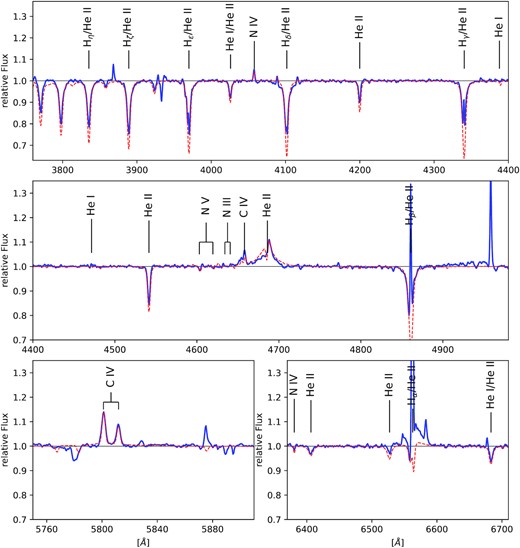
Spectroscopic analysis of Mk 33Na1 (OC2.5 If*). The blue line is the disentangled median spectrum (Section 3.1) while red the theoretical spectrum.
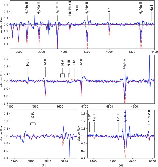
Spectroscopic analysis of Mk 33Na2 (O4 V). The blue line is the disentangled median spectrum (Section 3.1) while red the theoretical spectrum.
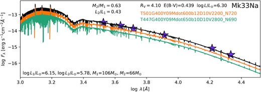
Combined and individual SEDs of Mk 33Na1,2 (solid-black, solid-orange, and cyan-green line). Derived luminosities based on the mass ratio derived using the orbital parameters (Section 2.3). Purple stars represent HST/WFC3 F336W, F438W, and F555W and VLT/MAD H and K-band photometry.
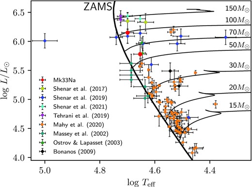
HRD of massive binary systems in the LMC. Binaries are included from this work (Mk 33Na), Shenar et al. (2017), Shenar et al. (2019), Shenar et al. (2021), Tehrani et al. (2019), Mahy et al. (2020), Massey et al. (2002), Ostrov & Lapasset (2003), and Bonanos (2009). Non-rotating evolutionary tracks and zero-age main-sequence isochrone are from Brott et al. (2011) and Köhler et al. (2015).
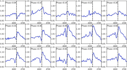
LPVs of He ii 4686 of all epochs as a function of phase.
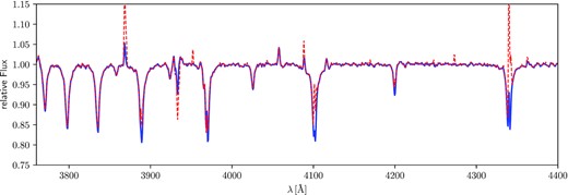
Blue-solid line is the primary median spectrum while red-dashed line is the averaged spectrum over all epochs (shift and add). Both spectra are similar, but the averaged spectrum (red-dashed line) contains more artefacts.
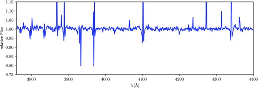
Random epoch divided by the primary median spectrum. The spectrum largely shows the spectral features of the secondary.
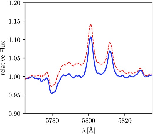
Blue solid is the primary median spectrum with removed broad C iv 5801-12 emission caused by the WC4 star Mk33Sb. Red-dashed line includes the broad C iv emission.
