


ABSTRACT
Since it was proposed, the exomoon candidate Kepler-1625 b-I has changed the way we see satellite systems. Because of its unusual physical characteristics, many questions about the stability and origin of this candidate have been raised. Currently, we have enough theoretical studies to show that if Kepler-1625 b-I is indeed confirmed, it will be stable. Regarding its origin, previous works indicated that the most likely scenario is capture, although conditions for in situ formation have also been investigated. In this work, we assume that Kepler-1625 b-I is an exomoon and study the possibility of an additional, massive exomoon being stable in the same system. To model this scenario, we perform N-body simulations of a system including the planet, Kepler-1625 b-I, and one extra Earth-like satellite. Based on previous results, the satellites in our system will be exposed to tidal interactions with the planet and to gravitational effects owing to the rotation of the planet. We find that the satellite system around Kepler-1625 b is capable of harbouring two massive satellites. The extra Earth-like satellite can be stable in various locations between the planet and Kepler-1625 b-I, with a preference for regions inside |$25\, R_{\rm p}$|. Our results suggest that the strong tidal interaction between the planet and the satellites is an important mechanism to ensure the stability of satellites in circular orbits closer to the planet, while the 2:1 mean motion resonance between the Earth-like satellite and Kepler-1625 b-I would provide stability for satellites in wider orbits.
1 INTRODUCTION
Natural satellites are common in our Solar system, and only two planets, Mercury and Venus, do not host any. The variety of satellites around planets is also remarkable. Regarding the size of satellites, there are larger satellites, such as the Galilean satellite Ganymede, which is larger than Mercury, and much smaller satellites, such as the inner Uranian satellites. Several special dynamical configurations are also found among the satellites of our Solar system; for example, there are satellites in resonance, most famously the three-body resonant chain, called the Laplace resonance, locking the motion of Io, Europa and Ganymede, and co-orbital satellites, such as the Janus–Epimetheus case around Saturn. In addition, it is not only planets that have satellites: in our Solar system, satellites are spotted around dwarf-planets, the famous Pluto–Charon binary system for example, and even around asteroids, such as in the case of the asteroid 65803 Didymos with its satellite Dimorphos (this system is the target of NASA’s mission DART (Double Asteroid Redirection Test), launched on 2021 November 24).
The abundance and diversity of detected exoplanets suggest the possibility of an equally diverse population of extrasolar satellites, termed exomoons. To date, no exomoons are confirmed, even though many candidates have been proposed (Bennett et al. 2014; Ben-Jaffel & Ballester 2014; Lewis et al. 2015; Hippke 2015; Teachey, Kipping & Schmitt 2018; Heller, Rodenbeck & Bruno 2019; Oza et al. 2019; Fox & Wiegert 2021). The absence of confirmed exomoons is due mainly to the limitations of present technology and instruments. Given these constraints, only exomoons with masses greater than 0.1–0.5 Earth masses (M⊕) could be detected by transit (Heller et al. 2014), currently one of the most promising methods for the detection of exomoons. This lower limit for the mass covers bodies that are one order of magnitude more massive than the most massive satellite of our Solar system, Ganymede.
Exomoons are a subject of interest in part because they are potentially habitable. Heller et al. (2014) point out that, because of the number of Jupiter-like planets inside their respective stellar habitable zones, exomoons could be more likely to harbour biological life than exoplanets. Zollinger, Armstrong & Heller (2017) showed that Mars-like satellites around giant planets in low-mass star systems could be good candidates for habitability under certain assumptions. More recently, Ávila et al. (2021) explored the case of an Earth-like satellite around a ‘free-floating’ Jupiter-like planet and found that a significant amount of liquid water can be retained on the exomoon’s atmosphere, and thus considered the simulated exomoons as capable of sustaining life.
Among the proposed exomoons, the most promising candidate is the one first presented by Teachey et al. (2018). These authors analysed the transit light curves from the Kepler telescope of the system Kepler-1625 and found signs of a Neptune-like satellite orbiting a giant planet. However, the analysis presented by Teachey et al. (2018) was based on only three transits of the planet. To confirm or refute the hypothesis of the exomoon’s presence, Teachey & Kipping (2018) combined the transits from Kepler with one more transit signal from the Hubble Space Telescope (HST). They found that the new data supported the hypothesis of a moon around Kepler-1625 b. Furthermore, they were able to refine the possible semimajor axis of the candidate and the mass of the planet.
The exomoon candidate hypothesis was contested by Kreidberg, Luger & Bedell (2019), who presented a re-analysis of the HST observations using an independent data reduction method. They showed that the transit light curve was well fitted by a planet-only model, so that the addition of a moon did not improve the fit. Moreover, Kreidberg et al. (2019) concluded that the moon signal found by Teachey et al. (2018) were merely an artefact from data reduction.
Heller et al. (2019) also aimed to contribute to the debate. These authors presented an alternative interpretation for the Kepler and HST data previously analysed. Using an independent reduction method for the HST data and the transits from Kepler, Heller et al. (2019) found a solution that corroborated the planet–moon scenario initially proposed; however, they pointed out that this result should be viewed with caution because of the systematic errors in the data from Kepler and HST. It was suggested that the presence of an exomoon is not a secure detection and that alternative interpretations from the data could be considered; for example, that the later transit by Kepler-1625 b could be due to the presence of a non-detected inclined inner planet. In this case, the planet will be a hot Jupiter with its mass depending on the considered semimajor axis.
More recently, Teachey et al. (2020) applied different detrending models to the transit light curves presented in Teachey & Kipping (2018) and found that some reduction techniques are indeed capable of smoothing the moon signal. However, from a statistical point of view, the adoption of more flexible detrending models did not provide better evidence than simpler detrending models, pointing in favour of a planet–moon scenario. Furthermore, Teachey et al. (2020) investigated the differences between the analyses of Teachey & Kipping (2018) and Kreidberg et al. (2019) and could not find the source of the discrepancies between the two results. In this way, the authors argued that the noise properties from the two analyses were identical, such that the light curves presented by Kreidberg et al. (2019) are not better constrained than those published first.
All in all, the current status of the problem is undetermined, with the planet–exomoon model being a valid interpretation for the signal identified in the Kepler and HST data.
Despite having an exomoon candidate, the Kepler-1625 system seems very ordinary when compared with other exoplanetary systems. It is formed by a G-type star with mass M⋆ ∼ 1.079 M⊙ and radius R⋆ ∼ 1.793 R⊙ (Mathur et al. 2017). So far, only one planet has been detected in the system, Kepler-1625 b. The planet has a semimajor axis of ap ∼ 0.87 au (Morton et al. 2016) and a radius of |$R_{\rm p} \sim 1.18\, R_{\rm J}$|. The planet’s mass is not well constrained, but previous investigations suggested a planet with a few Jupiter masses. Recent estimations presented by Teachey et al. (2020) show a peak probability around |$3\, M_{\rm J}$|. However, as shown in fig. 10 in Teachey et al. (2020), the distribution encompasses a broad range of values. The characteristics of the satellite candidate Kepler-1625 b-I are also not well determined. According to Teachey & Kipping (2018), the candidate is a Neptune-like body. Several planet–satellite orbital separations have been proposed based on different analyses (Teachey et al. 2018; Teachey & Kipping 2018; Martin, Fabrycky & Montet 2019; Teachey et al. 2020). In this paper, we will adopt the canonical value of |$40\, R_{\rm p}$|. The exomoon candidate’s orbit is usually assumed to be circular. The transit data indicate that the satellite would be in a very inclined configuration. Teachey & Kipping (2018) found that the inclination of the candidate is |$42^{+15}_{-18}$| degrees for a linear detrending, |$49^{+21}_{-22}$| degrees for a quadratic detrending, and |$43^{+15}_{-19}$| degrees for an exponential detrending. As can be seen, the inclination varies depending on the model adopted, and the error bar for the values is also very significant.
Since the proposal of Kepler-1625 b-I, many theoretical models have studied its stability (Heller 2018; Quarles, Li & Rosario-Franco 2020; Rosario-Franco et al. 2020) and origin (Hamers & Portegies Zwart 2018; Heller 2018; Hansen 2019; Moraes & Vieira Neto 2020). From the stability point of view, the satellite candidate is possible and stable, because its orbit is well inside the planet’s Hill sphere but not close enough for it to be dragged towards the planet as a result of tidal forces. The origin of this candidate, however, remains mysterious. Most papers focus on capture mechanisms for its origin, which is a fair assumption based on the satellite’s size, mass and inclination. Moraes & Vieira Neto (2020) found that formation in a circum-planetary disc is also possible, and the authors set a lower limit for the number of solids needed for the formation of such a massive body and studied its post-formation evolution. Their conclusion points towards in situ formation in a supermassive circum-planetary disc. However, the origin of the material was not discussed in their paper.
Based on the features of our Solar system, systems with multiple satellites are expected to be abundant around giant planets. The question is whether this pattern holds for exomoons around giant planets and how big these bodies could be. Many authors have studied the stability of single planet-sized satellites (Heller et al. 2014; Heller & Pudritz 2015a, b; Barr 2016), with most studies showing that Mars-like exomoons could be stable around super-Jovian planets. However, is this true for systems with multiple satellites?
Kollmeier & Raymond (2019) and Rosario-Franco et al. (2020) explored this issue when they discussed the feasibility of the moon’s moons, or submoons, around Kepler-1625 b-I. Even though submoons are not found in our Solar system, the size and orbital characteristics of Kepler-1625 b-I motivated Kollmeier & Raymond (2019) to study the stability around the satellite candidate and under what conditions a submoon would be stable. The authors found that the existence of submoons strongly depends on the mass of the host moon and its orbital separation from the planet, because of the intense tidal interactions between the submoon and the moon. They found that submoons are possible around Kepler-1625 b-I and that the largest possible submoon would have the Vesta-to-Ceres size. Later, Rosario-Franco et al. (2020) found that submoons around Kepler-1625 b-I will orbit inside a 0.33 Hill radius of the satellite (see their table 1 for more details), and the mass of the stable submoons would be |$70{{\ \rm per\ cent}}$| of the mass of the asteroid Vesta.
Moraes & Vieira Neto (2020) showed that even in an extreme system like Kepler-1625 b, multiple satellites could be stable for long periods in certain locations around the host planet. However, the authors did not explore in detail the locations of these bodies or the gravitational interaction between the surviving satellites.
Kipping (2021) identified a phenomenon that would be produced by the presence of one exomoon over the transit timing variation (TTV) of an exoplanet, the ‘exomoon corridor’. According to this author, the analysed TTVs induced by an exomoon will peak near two cycles. In addition, the author estimated that almost half of the exomoons would manifest themselves in short TTV periods of two to four cycles, regardless of the exomoon’s semimajor axis distribution (see fig. 1 from Kipping 2021). If this is the case, the exomoon corridor phenomenon will help to distinguish the TTVs induced by exomoons from those induced by planet–planet interactions. However, the exomoon corridor was developed for only one exomoon around a planet.
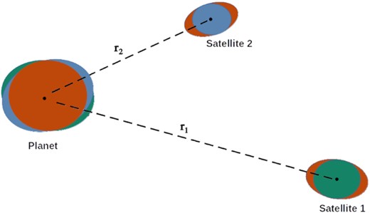
Illustration of how tides are considered in this paper. The central planet exerts tides on each satellite independently, and each satellite also exerts tides on the planet, but satellites do not generate tides in each other.
A recent study by Teachey (2021) expanded the exomoon corridor method to systems with multiple satellites and found that such an effect holds for systems with up to five satellites in both resonant and non-resonant configurations.
Motivated by the aforementioned works, we propose to investigate in more detail the regions around the planet Kepler-1625 b considering the presence of the satellite Kepler-1625 b-I, searching for orbits where other massive satellites would be stable.
We refer to ‘stable orbits’ in our systems as orbits where a secondary satellite can be placed and survive both the gravitational effects of the planet and the primary satellite (Kepler-1625 b-I) and the non-gravitational effects, such as tidal interactions with the central planet and the rotational deformation on the shape of the host body. We chose to take into account tides raised by the planet in the satellites and vice versa, and the rotational flattening effects from the planet, where such effects will be modelled by an estimation of the J2 coefficient of the body (Hussmann et al. 2019; Moraes & Vieira Neto 2020).
The paper is organized as follows. In Section 2, we detail the characteristics of the system and the equations of motion, and present a deeper discussion about the tidal and the rotational flattening models. Our models and results regarding the stability of the satellites are presented in Section 3; the analysis of the dynamical evolution of our system is given in Section 4; and in Section 5 we summarize our findings and draw our conclusions.
2 MODEL
Our main goal is to find stable orbits for massive satellites around Kepler-1625 b, considering that the satellite candidate Kepler-1625 b-I is already present. In this case, we will refer to Kepler-1625 b-I as the ‘primary satellite’, while the satellite for which we will study the stability will be identified as the ‘secondary satellite’.
The study proposed here is supported by previous studies targeting the possibility of finding multiple extrasolar satellites (Heller et al. 2016; Moraes & Vieira Neto 2020; Teachey 2021). Also, from the point of view of the origins of Kepler-1625 b-I, three scenarios have been proposed so far: tidal capture by the planet (Hamers & Portegies Zwart 2018); ‘pull-down capture’ from a co-orbital configuration (Hansen 2019); and in situ formation (Moraes & Vieira Neto 2020). In all cases, the hypothesis of having more satellites in the system is plausible. In the case of capture, Kepler-1625 b-I could have destroyed an ancient family of satellites around the host planet, pushed the ancient exomoons to closer orbits or scattered those satellites in wide eccentric orbits, somewhat similar to the scenario proposed for the capture of Triton in the Neptune system (Agnor & Hamilton 2006). In the case of in situ formation, Moraes & Vieira Neto (2020) identified surviving satellites that formed at the same time as Kepler-1625 b-I and are stable in inner orbits.
Because of the many uncertainties regarding the values for the mass, radius and semimajor axis of both Kepler-1625 b and Kepler-1625 b-I, in this paper we will consider some canonical values, as summarized in Table 1, where the mass and the radius of the satellite are given in terms of the mass and radius of Neptune, MNep and RNep, respectively. Because the information about the eccentricity and inclination of Kepler-1625 b-I is uncertain, we will consider the primary satellite to be in a circular and coplanar orbit around the central planet. Even though the analysis of the transits of Kepler-1625 b presented by Teachey & Kipping (2018) found that the exomoon candidate could be in a very inclined orbit, it is not yet possible to know if the planet is tilted on its axis, such that the exomoon’s orbit is coplanar with its equator, or if the exomoon candidate is indeed significantly inclined with respect to the planet’s equator. Here we have opted for the simpler case, where the exomoon is coplanar to the planet’s equator, and leave the inclined case for future explorations.
Canonical values of the mass, radius and semimajor axis adopted for the planet Kepler-1625 b and the satellite Kepler-1625 b-I (the data for the satellite describe a Neptune-size body at |$40\,R_{\rm p}$|).
| Mass | Radius | Semimajor axis | |
|---|---|---|---|
| [MJ ] | [RJ] | [ua] | |
| Kepler-1625 b | |$3$| | |$1.18$| | 0.87 |
| Kepler-1625 b-I | |$0.05395$| | |$0.3522$| | |$0.02206$| |
| Mass | Radius | Semimajor axis | |
|---|---|---|---|
| [MJ ] | [RJ] | [ua] | |
| Kepler-1625 b | |$3$| | |$1.18$| | 0.87 |
| Kepler-1625 b-I | |$0.05395$| | |$0.3522$| | |$0.02206$| |
For the secondary satellite, we opted to work with an Earth-like satellite (Table 1) because of the limitation imposed on the size of detectable satellites. In addition to Earth-like satellites, Ganymede- and Mars-like satellites were also tested in the early stages of our study. However, the differences in the size of these three types of satellites were not reflected in our results, and therefore we will only present the models with Earth-like bodies as the secondary satellites.
2.1 Equations of motion
As can be seen from equation (1), the presence of the star is neglected. As shown by Moraes & Vieira Neto (2020), for the distances we are considering for the satellites, the effects of the star can be safely ignored, as the planet will be the gravitationally dominant body.
2.2 Tidal and rotational flattening models
In addition to the gravitational interaction between the bodies in the system, we also assume tidal forces and rotational flattening as sources of perturbation on the system.
2.2.1 Tidal model
To properly model the tides in the system, we consider the constant time-lag formalism proposed in Mignard (1979) and Hut (1981) (see also Bolmont et al. 2015 and references therein). In our models we consider that the central planet will generate a tidal bulge in each satellite and that each orbiting satellite will also generate a tidal bulge in the central planet, while the satellites do not generate tides in each other (Fig. 1). Also, the tidal bulge induced by the planet on one satellite does not affect the motion of the other. On the other hand, all the bulges generated by the satellites on the planet affect the motion of all the orbiting bodies.
The tides have the effect of damping the eccentricity of the orbiting body while affecting its migration. The direction of the migration depends primarily on the eccentricity of the orbiting body and its semimajor axis.
As mentioned above, in all our models we will consider the central planet, the primary satellite Kepler-1625 b-I, and a secondary Earth-like satellite. To properly account for tides in the system, some important parameters must be set, namely the rotation period, the second-order potential Love number, and the constant time lag (hereafter referred to as tidal parameters) for each body. For simplicity, we will consider the central planet Kepler-1625 b to have tidal parameters equal to those of Jupiter (parameters taken from Bolmont et al. 2015). This choice is justified because the planet has a similar size to Jupiter and mass |$3\, M_{\rm J}$|. For a more massive planet (≥ 10 MJ), brown-dwarf parameters could be considered. For Kepler-1625 b-I, we follow Tokadjian & Piro (2020) and set the potential Love number and constant time lag to describe an ice-giant planet like Neptune, with k2, 1 = 0.34 and |$\tau _1 = 0.766\, {\rm s}$|. Also, the rotation period of the satellite was taken as 16 h, the same as for the planet Neptune. As the primary satellite is located farther out in the system, where the tides from the planet are weaker, a slower or faster rotating body will produce similar results. In the case of the secondary satellite, we are taking it to be an Earth-like body with the same tidal parameters as the Earth (values taken from Bolmont et al. 2015). We also tested an Earth-like satellite rotating faster (18 hours) and slower (30 hours); however, the results were very similar to those obtained with the typical rotation period of 24 h. A summary with the values of the tidal parameters for each body is presented in Table 2.
| Period | k2 | τ | |
|---|---|---|---|
| [h] | [s] | ||
| Kepler-1625 b | 10 | 0.380 | 1.842 × 10⁻³ |
| Kepler-1625 b-I | 16 | 0.340 | 0.766 |
| Secondary satellite | 24 | 0.305 | 698 |
| Period | k2 | τ | |
|---|---|---|---|
| [h] | [s] | ||
| Kepler-1625 b | 10 | 0.380 | 1.842 × 10⁻³ |
| Kepler-1625 b-I | 16 | 0.340 | 0.766 |
| Secondary satellite | 24 | 0.305 | 698 |
| Period | k2 | τ | |
|---|---|---|---|
| [h] | [s] | ||
| Kepler-1625 b | 10 | 0.380 | 1.842 × 10⁻³ |
| Kepler-1625 b-I | 16 | 0.340 | 0.766 |
| Secondary satellite | 24 | 0.305 | 698 |
| Period | k2 | τ | |
|---|---|---|---|
| [h] | [s] | ||
| Kepler-1625 b | 10 | 0.380 | 1.842 × 10⁻³ |
| Kepler-1625 b-I | 16 | 0.340 | 0.766 |
| Secondary satellite | 24 | 0.305 | 698 |
2.2.2 Rotational flattening model
Following Hussmann et al. (2019) and Moraes & Vieira Neto (2020), we chose to include in our models the effects of the non-sphericity of the simulated bodies due to their rotation.
In addition to the distortions on the surface of a body due to tides, the shape of this body will also change as a result of its rotation. The gravitational effects of this rotational deformation will change its gravitational field, thus affecting all the bodies in the system, especially those in closer orbits (Murray & Dermott 1999).
Here we consider the torques exerted by the planet on the satellites and the torques exerted by the satellites on the planet, while torques from one satellite are not felt by the other satellite. These gravitational effects will precess the orbit of eccentric satellites, causing the mean eccentricity and mean obliquity of the satellites to change (Bolmont et al. 2015).
3 NUMERICAL SIMULATIONS
Our study is mainly numerical, and thus we start this section by presenting the numerical tools used in this work, followed by a discussion about the systems studied and the results of our simulations regarding the stability of the systems. The analysis of the dynamical evolution of the systems is presented in Section 4.
3.1 Numerical tools
In this work we will perform N-body simulations using the numerical package posidonius1 (Blanco-Cuaresma & Bolmont 2017). posidonius is a new N-body code that allows the user to include dissipative effects such as tides, general relativity, rotational flattening, and the evolution of the bodies. The package is the second generation of the widely used mercury-t (Bolmont et al. 2015) written in Rust (see Blanco-Cuaresma & Bolmont 2016 for the advantages of using Rust in astrophysics) with a package of python scripts for the implementation of initial conditions and post-processing analysis. This new numerical tool ensures memory safety, can reproduce numerical N-body experiments, and improves the integration of the spin when compared with mercury-t. posidonius has been used in recent studies involving the evolution of planets and satellites in scenarios where tides are considered (Bolmont et al. 2019, 2020).
posidonius allows the user to choose between different integration schemes for the time evolution of the equations of motion. Here, we opted to use the ias15 integration scheme (Rein & Spiegel 2015). The main reason for this choice is that in our problem we expect to find several close encounters between the satellites and between the satellites and the central planet . The ias15 integrator can solve such close encounters with high accuracy while still being faster than most other high-order integration schemes (Rein & Spiegel 2015).
3.2 Initial conditions
As noted above, the systems we are studying are composed of the central planet (Kepler-1625 b), the primary satellite (Kepler-1625 b-I), and a secondary Earth-like satellite. The physical characteristics of the planet and the primary satellite are given in Table 1, while the secondary satellite has Earth’s radius and mass. The primary satellite starts at |$40\, R_{\rm p}$| from the planet for all cases, and in a circular and coplanar orbit. In order to find stable orbits for the secondary satellite, we simulate several cases with the initial semimajor axis of the satellites varying from a0 = 5 to |$a_0 = 35\, R_{\rm p}$|, considering |$\Delta a_0 = 2\, R_{\rm p}$|. For each position we simulate 10 cases, varying the eccentricity of the secondary satellite from e0 = 0.0 to e0 = 0.9, with Δe0 = 0.1. The satellites are taken to be coplanar in all cases. The angular orbital elements of both satellites and their obliquities are set to zero. Regarding the obliquity of the satellites, as we are considering the effects of tides and rotational flattening in addition to the usual gravitational interactions, Bolmont et al. (2015) showed for several cases that the obliquity of orbiting bodies under these dissipative effects decreases to zero very quickly, in about 100 yr. We used their results to justify our choice.
As we are considering additional effects to our model, we present the tidal parameters of all the bodies in the system in Table 2, recalling that we only consider tides generated by the planet on the satellites and the tides raised by the satellites on the planet, neglecting satellite–satellite tidal interactions. For the gravitational effects due to rotational flattening, the ‘only’ parameter needed is J2, which is calculated for each satellite and the planet with equation (7). Each simulation is carried out for 1 Myr or until a collision or an ejection is detected. Satellites are ejected from the system if they reach 1 Hill radius from the planet at any point. If a system survives for 1 Myr, we consider the system as stable; otherwise, the system is classified as unstable.
Hereafter we will refer to all systems by the initial semimajor axis and eccentricity of the secondary satellite.
3.3 Stability
In the following, we discuss our results regarding the stability of the systems when a secondary satellite is added. Also, we analyse the fate of the unstable systems.
In Fig. 2 we present our grid (semimajor axis versus eccentricity) of initial conditions. Green denotes stable initial conditions, and red denotes unstable ones. Later we will discuss the orbital evolution and the final configurations of the satellite systems, but for now it is important to note that even very eccentric initial conditions can provide long-term stable satellites owing to the effects of tides. As pointed out in the previous section, tides are a strong mechanism for damping the eccentricity of the orbiting bodies.
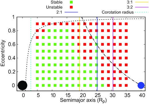
Grid with the initial conditions. Green denotes the conditions that end up being stable after 1 Myr, and red denotes the unstable cases. The vertical lines show the approximate locations of some mean-motion resonances, namely 2:1 (blue line), 3:2 (magenta line) and 3:1 (yellow line). The innermost dashed line shows the initial location of the corotation radius for the Earth-like moons. The black and blue circles represent the central planet and Kepler-1625 b-I, respectively. The black dashed line shows where the secondary satellites’ pericentres crosses the radius of the planet, and the black dash-dotted line shows where the secondary satellites’ apocentres crosses the orbit of the primary satellite.
From Fig. 2 we can see that the systems with the secondary satellite initially placed inside |$20\, R_{\rm p}$| are more likely to produce stable systems: this is the case because at these locations the gravitational effects of the primary satellite are weaker, and the evolution of the systems is dominated by the tidal interaction with the planet. Outside |$20\, R_{\rm p}$| the effects of the tides are weaker, and the gravitational perturbations from the primary satellite are more pronounced. At these locations, we see a decrease in the number of stable systems, especially among those with orbits that are initially eccentric. We note that secondary satellites in eccentric orbits are more likely to suffer a close encounter with the primary satellite, resulting in collisions or ejection from the system. In this way, the action of the tides as a mechanism to dampen the eccentricity of the secondary satellites is very important to reduce the probability of these close encounters.
For systems with the secondary satellite placed at distances greater than |$29\, R_{\rm p}$| we could not find stability. At these distances, the effects of the primary satellite are dominant, and close encounters that lead to the loss of the secondary satellites are common (the dash–dotted line in Fig. 2 shows the conditions for which the secondary satellites’ apocentre crosses the orbit of the primary satellite and close encounters are more likely). In addition, we will show later that the overlapping of resonances could create a chaotic region close to the primary satellite.
Also in Fig. 2 we present the initial location of three mean-motion resonances (MMRs), the 3:1 near |$19\, R_{\rm p}$|, the 2:1 near |$25\, R_{\rm p}$| and the 3:2 near |$31\, R_{\rm p}$|. These three MMRs play different roles in the stability of the systems. As can be seen, the 3:1 MMR is positioned inside a stable region, and thus the number of stable systems does not increase/decrease substantially because of the presence of the resonance. On the other hand, the 2:1 MMR is located in a transition region, where the number of stable systems decays. However, the system with secondary satellites starting near this region presents a increasing number of stable systems, which is directly correlated with the presence of the resonance. The outermost resonance we present is the 3:2 MMR slightly inside |$31\, R_{\rm p}$|. This region is too close to the primary satellite to be stable, and the MMR resonance does not contribute to the stability of the systems: most of the systems with the secondary satellite starting at |$31\, R_{\rm p}$| became unstable almost instantaneously. A more detailed study of the role the MMRs play in the systems will be presented in the next section.
To investigate the fate of the unstable systems, in Fig. 3 we show a diagram with only the unstable initial conditions, where the triangles represent a collision with the central planet, squares represent a collision with Kepler-1625 b-I, and circles represent ejection from the system. The colour bar on the right-hand side indicates the time it took for the system to become unstable, and the points marked in black are the conditions that become unstable instantaneously after the simulation starts.
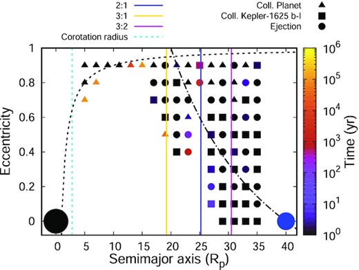
Grid with the unstable initial conditions of our models. The shape of the symbols indicates the fate of the satellite: triangles represent collision with the central planet, squares represent collision with the primary satellite (Kepler-1625 b-I), and circles represent ejection from the satellite system. The colour of the symbols indicates the time when the system became unstable according to the colour bar. The black dashed line shows where the secondary satellites' pericentres crosses the radius of the planet, and the black dash–dotted line shows where the secondary satellites' apocentres crosses the orbit of the primary satellite.
From Fig. 3 it can be seen that, as expected, the satellites initially in inner orbits are more likely to collide with the central planet. In the same way, satellites initially in wider orbits are more likely to collide with the primary satellite or be ejected from the system. However, satellites in wider eccentric orbits also collide with the planet: this happens because close encounters with the primary satellite end with the secondary satellite being pushed inwards, towards the planet, and a collision eventually takes place. We found several cases of ejections of the secondary satellites – the ejections are caused mainly by close encounters with the primary satellite (especially for secondary satellites located in outer regions) or by a resonant break.
Statistically, of the 160 different systems shown here, we found that exactly half of the systems are stable and half are unstable. For all the 80 unstable systems, we found that the most common fate was ejection, with 30 occurrences (|$37.5\, {{\ \rm per\ cent}}$|), followed closely by collision with the primary satellite, 29 cases (|$36.25\, {{\ \rm per\ cent}}$|), and collision with the central planet, 21 cases (|$26.25\, {{\ \rm per\ cent}}$|). Because the most unstable systems are found closer to the primary satellite, the most common reasons for instability being ejection and collision with this satellite are to be expected.
4 DISCUSSION
In this section, we focus on stable systems and discuss their dynamical evolution, such as migration, eccentricity damping and resonant configurations. In addition, we analyse the influences of the initial semimajor axis and eccentricity on our findings.
4.1 Migration and eccentricity damping
In Fig. 4 we show the final distribution of the semimajor axis versus eccentricity for our stable cases. When comparing the initial and final semimajor axes of the satellites, it can be seen that in most cases the satellites migrated inwards or were pushed inwards owing to a close encounter with the primary satellite. Notably, we found several cases of stability inside |$5\, R_{\rm p}$|, a region where the gravitational and tidal effects of the planet are stronger. These satellites present low eccentricities and will be long-term stable once they are outside their respective corotation radius, which means that there is no risk of these satellites colliding with the planet.
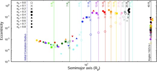
Final semimajor axis versus eccentricity distribution of the stable cases of our models. The models are separated by colour and shape. The colours identify the initial semimajor axis of the satellite (a0) from |$5\, R_{\rm p}$| to |$35\, R_{\rm p}$|, with |$\Delta a_0 = 2\, R_{\rm p}$|, as light-green (|$5\, R_{\rm p}$|), green (|$7\, R_{\rm p}$|), light-blue (|$9\, R_{\rm p}$|), blue (|$11\, R_{\rm p}$|), magenta (|$13\, R_{\rm p}$|), red (|$15\, R_{\rm p}$|), orange (|$17\, R_{\rm p}$|), yellow (|$19\, R_{\rm p}$|), pink (|$21\, R_{\rm p}$|), grey (|$23\, R_{\rm p}$|), black (|$25\, R_{\rm p}$|) and cyan (|$27\, R_{\rm p}$|). The vertical lines mark the initial semimajor axis by colour; the outermost vertical line marks |$40\, R_{\rm p}$|, the initial position of Kepler-1625 b-I. The shapes represent the initial eccentricity of the satellite (e0): 0.0 (open circle), 0.1 (cross), 0.2 (asterisk), 0.3 (square), 0.4 (filled circle), 0.5 (upward triangle), 0.6 (downward triangle), 0.7 (diamond) and 0.8 (pentagon). The bodies represented in the outermost vertical lines are the respective Kepler-1625 b-I for each case. The dashed dark-blue vertical line indicates the initial corotation radius of the system for the secondary satellite.
We found that the satellites migrating the most are those in initial eccentric orbits. Even though the secondary satellites are initially beyond the corotation radius of the system, because of their eccentric orbits the satellite tides prevail over the planetary tides, and in this case, as discussed above, the satellites migrate inwards until their eccentricity is damped to values below 0.1.
As an example, we show in Fig. 5 the evolution of the semimajor axis and eccentricity of the secondary (Earth-like) and primary (Kepler-1625 b-I) satellites for the case where the Earth-like satellite started at |$13\, R_{\rm p}$|. The evolution of the semimajor axis and eccentricity of the secondary satellites are shown in the left-hand panels, while the same parameters for the primary satellites are presented in the right-hand panels. We differentiate each case by their initial eccentricity using a colour scheme: from e0 = 0.0 to e0 = 0.8 we have the colours light green, green, light blue, blue, magenta, red, orange, yellow, and pink, respectively. The evolution of the case with e0 = 0.9 is not displayed because it results in an unstable system.
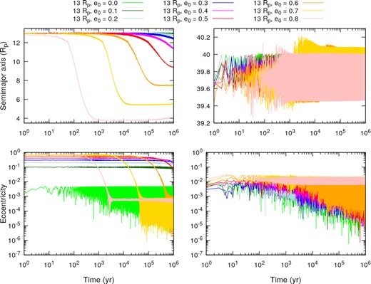
Time evolution of the semimajor axis and eccentricity of the primary and secondary satellites for the stable cases where the secondary satellites started at |$13\, R_{\rm p}$|. In the left-hand panels, we have the evolution of the semimajor axis (upper panel) and eccentricity (lower panel) of the secondary satellites. In the right-hand panels, we have the evolution of the semimajor axis (upper panel) and eccentricity (lower panel) of the primary satellites. The cases are separated by the initial eccentricity of the secondary satellites using a colour scheme: from e0 = 0.0 to e0 = 0.8 we have the colours light green, green, light blue, blue, magenta, red, orange, yellow and pink, respectively. The evolution of the case with e0 = 0.9 is not shown because it results in an unstable system.
As expected, the secondary satellites with initially higher eccentricity migrate inwards faster and reach inner orbits. In this phase, the migration of the eccentric satellites is determined by the satellite tides regime. As the satellites migrate towards the planet, their eccentricity is damped by the tidal interactions with the central body. As soon as the eccentricity of the satellites reaches small values, lower than 0.1 (Bolmont et al. 2011), the inward migration halts, and at this point the strength of the planetary tides overcomes the satellite tides, and the evolution of the semimajor axis of these bodies is determined by the planet–satellite spin ratio, which in the cases shown here results in a slow outwards migration. While the migration regime changes, the eccentricity of the satellites continues to decrease faster because of the proximity to the planet. Eventually, this decrease in the eccentricity stops, and the eccentricity of the satellites reaches a non-zero equilibrium range of values.
It is worth mentioning the role of Kepler-1625 b-I in the evolution of the system. From the right-hand panel in Fig. 5 we see that the primary satellite's semimajor axis does not vary significantly. This is because these satellites are too far from the central planet to be tidally disturbed, and their interaction with the inner satellite did not affect their semimajor axis much. However, the eccentricities of the primary satellites are excited by the presence of the inner satellites. On the other hand, the presence of the outer satellites is the reason why the inner satellites never reach circular orbits, even with tidal damping acting on their eccentricities. Also, for the case where the secondary satellite started in a circular orbit (light green line in the bottom left-hand panel), we can see that the presence of Kepler-1625 b-I is crucial, as the secondary satellite’s orbit is perturbed and its eccentricity increases to values near 0.001 almost instantaneously. Nevertheless, this non-zero eccentricity does not translate to a significant change in the semimajor axis of the Earth-like satellite in this specific case.
The pattern exemplified in Fig. 5 was found in most of our simulations, except for the cases where the satellites were trapped in a resonance or pushed out of a resonant configuration. That is, all the cases where the secondary satellite had an initial semimajor axis smaller than |$17\, R_{\rm p}$| had a similar outcome to that described above. For systems with the secondary satellite initially in a wider orbit, a combination of weaker tidal forces and the presence of low-order MMR prevents the significant inward migration of the secondary satellite. In these cases, most of the satellites did not migrate much, and their final eccentricities are higher.
4.2 Resonances
In recent years, compact multiplanetary systems locked in resonances have been found (Mills et al. 2016; Luger et al. 2017; Leleu et al. 2021). According to Mills et al. (2016), the presence of MMRs in compact systems greatly helps the stability of the systems, exciting and stabilizing the eccentricity of the planets. In satellite systems, resonances also play a significant role, not only in the stability of the system but also in sculpting the final architecture of the system, the Laplace resonance presented by the Galilean system being the best-known example in our Solar system.
Here we will discuss the role that a few MMRs play in the stability of the systems.
4.2.1 Systems near the 3:1 MMR
We start our analysis with systems that are not in resonance but are very close. In Fig. 6 we show the evolution of the semimajor axis and eccentricity of the secondary and the primary satellites for the case where the Earth-like satellites start at |$19\, R_{\rm p}$|. As before, on the left-hand side we have the evolution of the semimajor axis and eccentricity of the secondary satellites, while on the right-hand side we have the same parameters presented for the primary satellites.
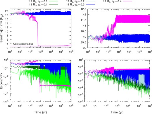
Time evolution of the semimajor axis and eccentricity of the primary and secondary satellites for the stable cases where the secondary satellites started at |$19\, R_{\rm p}$| (near the 3:1 MMR). In the left-hand panels, we have the evolution of the semimajor axis (upper panel) and eccentricity (lower panel) of the secondary satellites. In the right-hand panels, we have the evolution of the semimajor axis (upper panel) and eccentricity (lower panel) of the primary satellites. The cases are separated by the initial eccentricity of the secondary satellites using a colour scheme: from e0 = 0.0 to e0 = 0.4, with Δe0 = 0.1,we have the colours light green, green, light blue, blue, magenta, respectively. The evolution of the other cases is not shown because they result in unstable systems. The horizontal dashed line indicate the corotation radius.
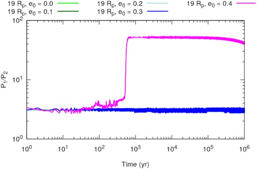
Time evolution of the satellites’ period ratio for the stable systems presented in Fig. 6 (near the 3:1 MMR).
For two bodies in resonance, one of the three angles described in equation (9) would be librating around one specific value. However, for all cases, the three angles were found to be circulating, which means that, despite the commensurability of the satellites’ orbital periods , the satellites are not locked in resonance. As an example of the time evolution of the resonant angles for these cases, we show in Fig. 8 the behaviour of |$\phi ^{(1)}_{3:1}$| for the cases where the secondary satellites started with eccentricities from e0 = 0.0 to e0 = 0.3; the case with e0 = 0.4 is not shown because the system is clearly out of a hypothetical MMR. The behaviours of |$\phi ^{(2)}_{3:1}$| and |$\phi ^{(3)}_{3:1}$| are similar to that of |$\phi ^{(1)}_{3:1}$|.
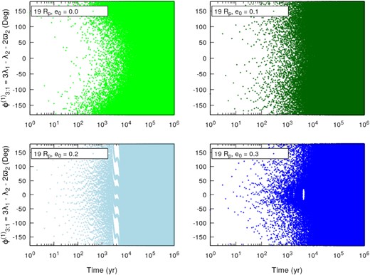
Time evolution of the resonant angle |$\phi ^{(1)}_{3:1} = 3\lambda _1 - \lambda _2 -2\varpi _2$| (first line in equation 9) for the stable cases where the secondary satellites started at |$19\, R_{\rm p}$| (near the 3:1 MMR). From top left to bottom right we have the cases separated by the initial eccentricity of the secondary satellites, from e0 = 0.0 to e0 = 0.3. The case with e0 = 0.4 was omitted from the graph because the system is clearly not in a MMR.
In this case, instead of a MMR locking the motion of the satellites, the semimajor axes and eccentricities of the satellites are not damped because at |$19\, R_{\rm p}$| the tidal effects coming from the planet are weak and the satellites preserve an orbital configuration similar to their initial conditions. Thus we cannot evaluate the role that the 3:1 MMR plays for the stability of the satellites, because the satellites near this resonance do not show any resonant behaviour.
Another important feature displayed in Fig. 6 is the behaviour of the secondary satellite that started with e0 = 0.4 (magenta line). Different from the other cases, this satellite escaped the region near the 3:1 MMR thanks to multiple close encounters with the primary satellite, as can be seen by the erratic behaviour of its semimajor axis, before a final encounter that resulted in the secondary satellite being pushed inwards. Because the damping effects of the tides on the satellite's eccentricity are stronger in the inner regions, the satellite’s orbit is almost circularized before the satellite reaches the corotation radius. After this abrupt process of circularization, the satellite starts to experience an outward migration, resulting from the tides generated by the planet.
Because the secondary satellites around |$19\, R_{\rm p}$| are not in MMR they are not free from a future close encounter with the primary satellite. As these satellites maintained high eccentricities during their evolution, a close encounter could take place at some point.
4.2.2 Systems locked in 2:1 MMR
As noted above, as we start the secondary satellites farther from the planet, the effects of the tides become weaker and the mutual gravitational interaction between the primary and secondary satellites is stronger. In this way, we found that when the secondary satellites start beyond |$20\, R_{\rm p}$|, the percentage of stable systems decreases steeply. At these outer locations, the migration rate and eccentricity damping induced by the tides are smooth, and the secondary satellites are more likely to suffer a disruptive close encounter with the primary satellite, especially the satellites in eccentric orbits. However, for the cases where the secondary satellites start at |$25\, R_{\rm p}$| a high number of systems are stable, which is due to the presence of a 2:1 MMR near this initial position.
In Fig. 9 we show the evolution of the semimajor axis and eccentricity of the primary and secondary satellites for a stable system when the secondary satellite starts at |$25\, R_{\rm p}$|. The high number of stable systems presented might be explained by the location of a 2:1 MMR with the primary satellite near the orbital distance where the satellites are initialized. Also, from Fig. 9 it can be seen that, despite small amplitudes, after 100 yr the semimajor axis of the secondary satellites does not change significantly. The same is true for the eccentricities of the satellites, which remain high in some cases.
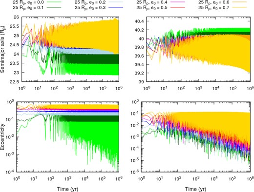
Time evolution of the semimajor axis and eccentricity of the primary and secondary satellites for the stable cases where the secondary satellites start at |$25\, R_{\rm p}$| (near the 2:1 MMR). In the left-hand panels, we have the evolution of the semimajor axis (upper panel) and eccentricity (lower panel) of the secondary satellites. In the right-hand panels, we have the evolution of the semimajor axis (upper panel) and eccentricity (lower panel) of the primary satellites. The cases are separated by the initial eccentricity of the secondary satellites using a colour scheme – from e0 = 0.0 to e0 = 0.7 we have the following colours: light green, green, light blue, blue, magenta, red, orange and yellow, respectively. The evolution of the cases with e0 = 0.8 and e0 = 0.9 are not shown because they result in unstable systems.
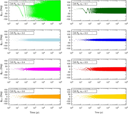
Time evolution of the resonant angle ϕ2: 1 = 2λ1 − λ2 − ϖ2 for the stable cases where the secondary satellites start at |$25\, R_{\rm p}$| (near the 2:1 MMR). From top left to bottom right we have the cases separated by the initial eccentricity of the secondary satellites, from e0 = 0.0 to e0 = 0.7.
The analysis of Fig. 10 is straightforward. The case where the Earth-like satellite is initialized in a circular orbit presents a circulating resonant angle, which means that the satellites are not locked in a MMR. From Fig. 9 it can be seen that this case is the one where the semimajor axis deviates the most from its initial value. The secondary satellite started at |$25\, R_{\rm p}$| has a close encounter with the primary satellite (which is clear given the increase in its eccentricity and sudden decrease in semimajor axis soon after 10 yr) and finds a stable, but not resonant, configuration around |$23\, R_{\rm p}$|.
Except for the case where the Earth-like satellite is initialized in a circular orbit, all other cases present a resonant angle librating around 0° with a maximum amplitude of 50°. This behaviour supports the claim that the satellites have their motion locked in a 2:1 MMR. Because the secondary satellites placed initially farther from the planet tend to become unstable with time, we argue that the 2:1 MMR between the satellites can be the dynamical mechanism ensuring the stability of these systems. On the other hand, in some resonant systems the secondary satellite is in a very eccentric orbit, which might lead to a disruptive close encounter and the break of the resonant configuration between the satellites: such a dynamical event could jeopardize the stability of the systems.
4.2.3 Unstable systems near the 3:2 MMR
Beyond |$25\, R_{\rm p}$| we have the presence of a 3:2 MMR resonance located near |$31\, R_{\rm p}$|. However, this region was found to be empty of stable systems. The systems with the secondary satellite starting at |$31\, R_{\rm p}$| became unstable almost instantaneously given the strong gravitational influence of the primary satellite. For these systems, the most common fate for the secondary satellite is a collision with the primary satellite (|$50{{\ \rm per\ cent}}$| of the systems), followed by ejection (|$30{{\ \rm per\ cent}}$|) and collision with the planet (|$20{{\ \rm per\ cent}}$|).
Another reason for the lack of stable systems in the 3:2 MMR location could be the overlapping of resonances. As the distances from the primary satellite are shortened, successive first-order resonances of the form p + 1: p will appear, each one independent of the other. As each resonance has a given width, at short distances from the exterior perturber these resonances will eventually start to overlap. As a consequence of this effect, chaotic motion could arise, leading to instability.
We point out that the regions of instability will change if the masses of the bodies considered and the initial radial separation of the primary satellite are different.
5 CONCLUSIONS
In this work, we have explored the dynamical stability of an Earth-like satellite in the Kepler-1625 b system, considering that the system already has a massive satellite, the Neptunian-like candidate Kepler-1625 b-I.
In this study, we tried to answer the following questions.
Given that Kepler-1625 b-I is stable, is it possible to have another massive moon in this system?
Are there preferred orbital configurations or locations for the extra satellite?
How will Kepler-1625 b-I dynamically affect this extra satellite?
To answer these questions, we performed N-body simulations considering a system formed by the central planet, Kepler-1625 b-I, and an extra Earth-sized satellite, using the N-body code posidonius. To accurately model the system, we took into account the tidal effects generated by the satellites on the planet and by the planet on the satellites, and the effects due to the rotational deformation of the simulated bodies.
We focused on the region between the planet and Kepler-1625 b-I (initially at |$40\, R_{\rm p}$|), such that we built a grid of initial conditions varying the semimajor axis and the eccentricity of the satellites. For the semimajor axis of the secondary satellites, we chose to place the innermost case at |$a_0 = 5\, R_{\rm p}$|, outside the corotation radius of the system, while |$a_0 = 35\, R_{\rm p}$| was taken as the outermost initial semimajor axis, using |$\Delta a_0 = 2\, R_{\rm p}$| as the width of our grid. For each initial semimajor axis we simulated 10 different cases, varying the eccentricity of the secondary satellite, from e0 = 0.0 to e0 = 0.9. We opted to include highly eccentric cases in our grid because we are considering the tidal effects on the satellites, which could dampen the eccentricity of such bodies to values close to zero. Thus, we have in total 160 different initial conditions.
Fig. 2 answers our first question. Yes, it is possible to have two massive satellites, an Earth-like and a Neptune-like satellite, around the planet Kepler-1625 b. We found that |$50{{\ \rm per\ cent}}$| of our simulations ended with a system with two satellites stable for 1 Myr. As expected, the satellites with initial high eccentricity and orbits closer to the planet suffered a collision with the central body almost instantaneously. The same was true for the satellites initially in wider orbits, closer to Kepler-1625 b-I. Our results show that the cases where the secondary satellites were initially within |$20\, R_{\rm p}$| have a higher chance of producing stable systems, even for initially eccentric configurations.
The second main question we try to answer is related to the final location of the surviving secondary satellites. We found that the primary satellite tends to remain at |$\sim 40\, R_{\rm p}$| for most of the cases, unless close encounters between the satellites take place. On the other hand, its orbit acquired some non-negligible eccentricity (between 0.001 and 0.1) due to the gravitational interactions with the inner satellites, even when close encounters are not found.
For the Earth-like satellites, our results showed that there is no preferred location for these satellites to be stable inside |$25\, R_{\rm p}$|. Beyond this limit, the satellite will be mostly unstable due to gravitational effects from the primary satellite, generating chaotic motion produced by resonance overlapping. For the surviving systems, we found that most of the secondary satellites migrated inwards, especially the eccentric satellites (owing to the action of the satellite tides).
In addition to the satellites that experience inward migration, we have satellites that for one reason or another do not present a significant migration. These satellites are either in circular orbits, too far away to experience strong tidal interactions with the planet, or are trapped in MMRs with the primary satellite.
The third main question we answer is related to the dynamical effects of Kepler-1625 b-I on an inner massive satellite. As mentioned above, most of the satellites initially placed closer to the primary satellite |$(a_0 \gt 25\, R_{\rm p})$| become unstable.
Our results show that MMRs are responsible for most of the stable systems when the secondary satellite starts at wider orbits. We kept track of satellites starting close to the 2:1, 3:2 and 3:1 MMRs. Only the 2:1 MMR effectively influenced the stability of the satellites. The 3:2 resonance was located too close to the primary satellite, and thus the satellites near this MMR were unstable. On the other hand, the stable satellites near the 3:1 commensurability never became locked in resonance, and this resonance did not protect the most eccentric satellites from being unstable.
In summary, our work shows that the satellite system around Kepler-1625 b could be even more fascinating than is currently predicted. The system has the potential to harbour not just one but two planet-sized satellites. This theoretical secondary satellite does not show a preferable location inside |$25\, R_{\rm p}$| and could be stable in almost-circular orbits close to the planet or in wider orbits locked in a MMR with Kepler-1625 b-I.
In this work, we have restricted ourselves to studying the stability of regions between the planet and the predicted location of Kepler-1625 b-I, leaving the study of regions beyond |$40\, R_{\rm p}$| and co-orbital configurations for future analysis. These two studies will be complementary to that presented here, because a more extended region of the system will be explored.
Furthermore, we have only studied the coplanar case, assuming that all bodies involved have zero inclination. However, Kepler-1625 b-I, if confirmed, is predicted to have a high inclination. In this case, an additional study taking into account inclined bodies is needed. We expect that the addition of inclined bodies will not affect the stability of the innermost surviving satellites because their evolution will be still dictated by the tides from the planet. On the other hand, the outer satellites will be more likely to be affected by an inclined body and eventually become inclined or unstable. Moreover, the stability of the outermost satellites relies on the appearance of MMRs: this could be an issue when inclined bodies are considered.
ACKNOWLEDGEMENTS
We thank the anonymous referee for their valuable comments and suggestions that helped to improve the quality of this paper. This work was possible thanks to the scholarship granted from the Brazilian Federal Agency for Support and Evaluation of Graduate Education (CAPES), in the scope of the Program CAPES-PrInt, process number 88887.310463/2018-00, mobility number 88887.583324/2020-00 (RAM). JM is grateful for financial support from The São Paulo Research Foundation - FAPESP (grant: 2019/21857-3). RAM, OCW and JM are grateful for financial support from FAPESP (grant: 2016/24561-0) and The National Council for Scientific and Technological Development - CNPq (grant: 305210/2018-1). This research was supported by resources supplied by the Center for Scientific Computing (NCC/GridUNESP) of São Paulo State University (UNESP).
DATA AVAILABILITY
The data underlying this paper will be shared on reasonable request to the corresponding author.
