


ABSTRACT
In this paper, which is the first in a series of papers devoted to a detailed analysis of ‘the death line’ of radio pulsars, we consider a possibility of producing secondary particles at a sufficiently long pulsar period P. To this end, we reconsidered the potential drop necessary for secondary plasma generation in the inner gap over magnetic polar caps. Our research made it possible to refine the conditions for generating secondary plasma, such as the multiplicity of the production of secondary particles and their spatial distribution. Our research also made it possible to further quantitatively analyse the dependence of the possibility of secondary plasma generation on all parameters, including the inclination angle of the magnetic axis to the rotation axis, the polar cap size and the magnetic field geometry.
1 INTRODUCTION
According to our modern understanding of the phenomenon of radio pulsars, their radio emission is associated with secondary electron–positron plasma generated in the polar regions of a neutron star (Sturrock 1971; Ruderman & Sutherland 1975; Arons 1982; Lorimer & Kramer 2012; Lyne & Graham-Smith 2012). It is therefore not surprising that the cessation condition of the generation of secondary particles is associated with the so-called ‘death line’ on the P–|${\dot{P}}$| (or P–B0) diagram, where P is the pulsar period, and B0 is the magnetic field at the magnetic pole.
Detailed works devoted to the generation of secondary plasma have been underway since the beginning of the eighties (Daugherty & Harding 1982; Gurevich & Istomin 1985; Arendt & Eilek 2002; Istomin & Sobyanin 2007; Medin & Lai 2010; Timokhin 2010; Timokhin & Arons 2013; Philippov, Spitkovsky & Cerutti 2015; Timokhin & Harding 2015; Cerutti, Philippov & Spitkovsky 2016). Nevertheless, up to now, a large number of different options are discussed in the literature (Ruderman & Sutherland 1975; Blandford & Scharlemann 1976; Arons 1982; Usov & Melrose 1995), leading to very different conditions which set ‘the death line’ of radio pulsars (Chen & Ruderman 1993; Zhang, Harding & Muslimov 2000; Hibschman & Arons 2001; Faucher-Giguére & Kaspi 2006; Konar & Deka 2019).
In this and the following article, we set ourselves the task of reconsidering all basic approximations usually used in constructing the secondary plasma production model, but which may work poorly near ‘the death line’. In particular, we assume that due to irregularity of the secondary plasma production, almost the entire region of open field lines can be considered in a vacuum approximation: ρe = 0. In other words, our task is to clarify the position of ‘the death valley’ (Chen & Ruderman 1993) using modern models of the magnetosphere structure and the deceleration of a neutron star; the latter is necessary to quantify the period derivative |${\dot{P}}$| in terms of P, B0, and the inclination angle χ. The effects of general relativity will also be taken into account.
Please note that in this work, the ‘classical’ mechanism of the particle production is considered due to the single-photon conversion of the γ-quantum into an electron–positron pair in a superstrong magnetic field. As is well known (Sturrock 1971; Ruderman & Sutherland 1975), this process includes primary particle acceleration by a longitudinal electric field, emission of γ-quanta due to curvature radiation, production of secondary electron–positron pairs, and, finally, secondary particle acceleration in the opposite direction, which also leads to the creation of secondary particles. In other words, we do not consider particle production due to Inverse Compton Scattering, which, as is well known (Blandford & Scharlemann 1976; Zhang et al. 2000), can also be a source of hard γ-quanta. As an excuse, we note that we will first of all be interested in old pulsars, in which the surface temperature may not be high enough to form a sufficient number of X-ray photons.
For the same reason, we do not take into consideration synchrotron photons emitted by secondary pairs. The point is that, as is well known (see, e.g. Gurevich & Istomin 1985; Istomin & Sobyanin 2007 and section 3.1 below), the energy of synchrotron photons emitted by secondary particles is approximately 15–20 times less than the energy of curvature photons emitted by primary particles. Therefore, near the threshold of particle production, when the free path length of curvature photons become close to the radius of the star R, the pulsar magnetosphere appears to be transparent for synchrotron photons.
It is clear that in the mid 70s, such accuracy was quite acceptable, especially since expression (5) was really limited from below most of the pulsars in the P–|${\dot{P}}$| diagram. However, as was already shown by Chen & Ruderman (1993), the standard RS model (dipole magnetic field, etc.) gives a very large period derivative |${\dot{P}}$| for the observed ‘death line’. That is why the idea was put forward to consider a more complex structure of the magnetic field resulting in a decrease of the period derivative (and leading to the appearance of ‘a death valley’). However, as was already emphasized, the observed period derivative |${\dot{P}}$| can be affected by many other reasons (masses and radii of neutron stars, the size of the polar cap, the effects of general relativity), which were not considered in the qualitative analysis carried out by Chen & Ruderman (1993). In particular, within the framework of this model, the simplest magnetodipole formula was used to determine the period derivative |${\dot{P}}$|, which, as it is now clear, does not correspond to reality. Therefore, one of the main tasks of our consideration is the question of what parameters can lead to a decrease in the observed deceleration rate |${\dot{P}}$|.
To clarify this issue, we consider an almost vacuum gap model of the polar region. Remember that all modern models of particle generation (including recent PIC simulations) implicitly assume free ejection of particles from the neutron star surface. Consequently, one could expect that the potential drop would be close to that predicted in the Arons (1982) model, i.e. much smaller than in the vacuum gap Ruderman–Sutherlend model. However, as was shown in recent works performed in the PIC simulation (Timokhin 2010; Philippov, Timokhin & Spitkovsky 2020), due to strong non-stationarity, vacuum regions appear from time to time, with the potential drop being close to the vacuum gap model. Particularly, such an assumption is natural for the pulsars located near ‘the death line’. In this case, the beginning of the cascade (and, hence, the filling of this region with a secondary electron–positron plasma) can be initiated by the cosmic gamma background, which, as is known, leads to 105–108 primary particles per second in the polar cap region (Shukre & Radhakrishnan 1982).
On the other hand, for the pulsars in the vicinity of ‘the death line’, the free path length lγ of γ-quanta leading to the production of secondary particles can be of the order of star radius R (the scale of the diminishing of the dipole magnetic field), i.e. much larger than the transverse size of the polar cap Rcap ∼ 0.01R. Therefore, we need to determine 3D potential resulting in the acceleration of primary particles.
Let us note straight away that below we consider only a dipole magnetic field despite a large number of works which indicated that it is impossible to explain ‘the death line’ in a dipole magnetic field (Arons 1993; Asseo & Khechinashvili 2002; Barsukov & Tsygan 2010; Igoshev, Elfritz & Popov 2016; Bilous et al. 2019). In other words, one of our tasks is to verify the possibility of explaining the position of ‘the death line’ by other factors which are usually not considered when analysing the processes of secondary plasma production. Among such possible factors, one can indicate a decrease in the magnetic field with distance from the star, the possibility of producing secondary pairs by γ-quanta whose energy is much larger than the typically used characteristic energy of the maximum of the spectrum, as well as the fact that secondary plasma is generated on field lines located closer to the magnetic axis than gamma-ray emitting particles. All these effects become significant near ‘the death line’ when the free pass length of γ-quanta becomes comparable to the radius of a neutron star. The role of the non-dipole magnetic field and all the other physical parameters which can affect the position of ‘the death line’, will be discussed in detail in Paper II.
As for Paper I, which is the first in a series of papers devoted to a detailed analysis of ‘the death line’ of radio pulsars, it is devoted to the possibility of producing secondary particles at sufficiently large periods P. In Section 2, we construct an exact three-dimensional solution for a longitudinal electric field E∥ in the polar regions of a neutron star in the case when plasma is absent in the entire region of open field lines. We show that in real dipole geometry for non-zero inclination angles χ, the longitudinal electric field decreases much slower than previously assumed. In addition, the corrections related to the effects of general relativity are determined. Further in Section 3, we show that close to ‘the death line’ a major role in particle creation begin to play those γ-quanta whose energy is several times greater than the commonly used characteristic energy of curvature radiation. Finally, in Section 4, the generation of secondary electron–positron pairs near ‘the death line’ is considered when the second-generation particles produced by the conversion of synchrotron photons can be neglected. Section 5 is devoted to the conclusion and discussion.
2 ALMOST VACUUM GAP
2.1 Potential drop
Here the following points should be stressed.
- The expressionin (17) is indeed the exact asymptotic solution at large distances from the star surface (r − R) ≫ R0 in the dipole magnetic field (certainly, in the limit θ ≪ 1).(32)$$\begin{eqnarray} \psi (r, \theta , \varphi) & = & \frac{1}{2} \, \frac{\Omega B_{0}R_{0}^2}{c}\left[1-\frac{\theta ^2}{\theta ^2_{0}(r)}\right]\cos \chi \\ && + \, \frac{3}{8} \, \frac{\Omega B_{0}R_{0}^2}{c}\, \left[\theta -\frac{\theta ^3}{\theta ^2_{0}(r)}\right]\sin \varphi \sin \chi \end{eqnarray}$$
At large distances (r − R) ≫ R0, the magnetic field lines θ(r) ∝ r1/2 become equipotential only for the symmetric component of the potential ψ. For the anti-symmetric (φ-dependent) part realizing for any oblique rotator with χ ≠ 0°, the longitudinal electric field decreases on the scale of the star radius R, not the polar cap radius R0. We emphasize that this effect does not exist for a model of the conical geometry of open magnetic field lines when θ0 = const.
- As a result, one can obtain for the anti-symmetric component of the potentialwhere again l denotes the coordinate along the magnetic field line, and we use the dimensionless area 0 < f < f*. As we see, the additional potential drop within the light cylinder ψ(l = RL) is the same as the characteristic vacuum potential within the polar cap.(33)$$\begin{eqnarray} \psi (l) = \frac{3}{8} \, \left(\frac{f}{f_{\ast }}\right)^{1/2} \left(1 - \frac{f}{f_{\ast }}\right) \, \frac{\Omega B_{0}R_{0}^3}{c R} \left(\frac{l}{R}\right)^{1/2} \sin \varphi \sin \chi , \end{eqnarray}$$
- Accordingly, the additional parallel electric field looks like(34)$$\begin{eqnarray} E_{\parallel }^{\rm add} = -\frac{3}{16} \, \left(\frac{f}{f_{\ast }}\right)^{1/2} \left(1 - \frac{f}{f_{\ast }}\right) \, \frac{\Omega B_{0}R_{0}^3}{c R^2} \left(\frac{l}{R}\right)^{-1/2} \sin \varphi \sin \chi . \\ \end{eqnarray}$$
Previously, no one paid attention to the existence of an additional longitudinal field for the case of an oblique rotator when the dependence of the boundary of the region of open field lines on the distance to the star becomes significant. In particular, in the famous work of Muslimov & Tsygan (1992), a change of variables ξ = θ/θ0(r) was made when solving the equation (11), but in what follows, the dependence θ0(r) on r was not taken into account.
2.2 Particle acceleration
It should be immediately noted that due to the additional factor R0/R, this component of the longitudinal electric field becomes significant near the surface of the neutron star for the inclination angles cos χ ∼ R0/R only. Fig. 1 shows the values of the Lorentz-factor |$\gamma = {\cal E}_{\rm e}/m_{\rm e}c^2$| of a particle accelerated from the surface of a neutron star from the point f = 0.7 and φ = 90° obtained by solving the equation (35) for two values of the pulsar period P = 0.3 s (upper curves) and P = 1 s (lower curves) for small (χ = 30°, top) and large ( χ = 85°, bottom) inclination angles. The dashed lines show the solutions in which the additional electric field ( 34) is neglected. As we see, the role of the additional electric field becomes noticeable only for almost orthogonal rotators.
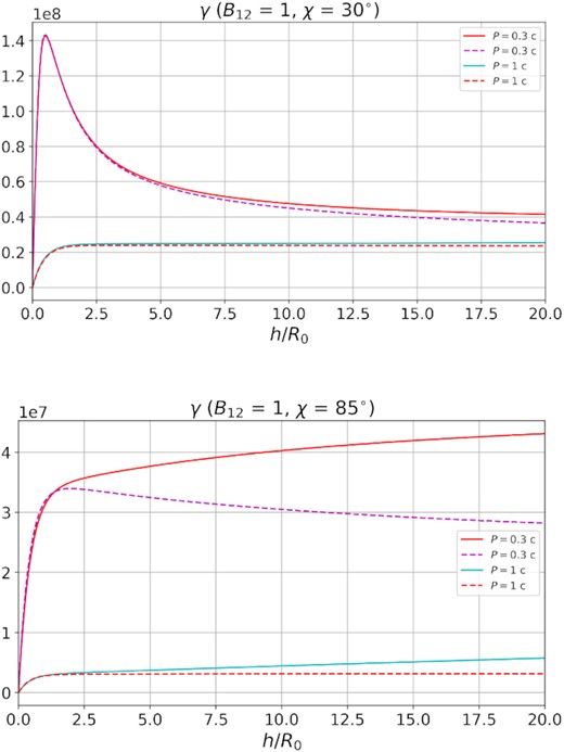
Lorentz-factor |$\gamma = {\cal E}_{\rm e}/m_{\rm e}c^2$| of a particle accelerated from the surface of a neutron star obtained by solving the equation (35) for two values of the pulsar period P = 0.3 s and P = 1 s for small (χ = 30°, top) and large (χ = 85°, bottom) inclination angles. The dashed lines for each of the two periods show the solutions in which the additional electric field (34) is neglected.
However, for us, it is much more important that for pulsars with relatively large periods P ∼ 1 s, i.e. just near ‘the death line’, the energy losses of a particle described by the second term in the equation (35) becomes negligible. Therefore, the lower curves in Fig. 1 correspond to the electric potential ψ(l). For this reason, in what follows, for such pulsars, we can simply put |${\cal E}_{\rm e}(l) = e \psi (l) - e\psi (l_{0})$|, where l0 corresponds to the particle creation point. For shorter periods P, the particle energy does not reach the maximum possible energy eψ, and subsequently decreases with increasing the distance from the neutron star surface.
2.3 General relativistic correction
As is well known, the effects of general relativity and, in particular, the frame-dragging (Lense-Thirring) effect, under certain conditions, can play a significant role in the generation of secondary plasma near the polar caps of the neutron star (Beskin 1990; Muslimov & Tsygan 1992; Philippov et al. 2015, 2020). For this reason, below, we estimate all possible corrections which can affect the production of secondary particles. For simplicity, we restrict ourselves to only the first order in the small parameter rg/R, where rg = 2GM/c2 is the black hole radius.
Thus, as expected, we can conclude that the effects of general relativity lead to corrections at the level of 10–20 per cent. Consequently, the corresponding corrections at first glance do not go beyond the uncertainty in other quantities, such as, e.g. the radius and moment of inertia of a neutron star. Nevertheless, below, we include general relativity corrections into consideration since, as will be shown, these corrections lead to a significant change in the rate of production of secondary particles.
3 GENERATION OF CURVATURE PHOTONS
3.1 Effective photon energy
As shown in Table 1, even for the characteristic parameters, the most effective frequency ω = ξωc is indeed higher than ωc (48). As for the pulsars located within ‘the death valley’, their effective frequency can be sufficiently higher. In Table 2, we show the parameters |${\cal K}$| and ξ for some of these pulsars. Their parameters were taken from the ATNF catalog (Manchester et al. 2005), and the appropriate Lorentz-factors correspond to the potential drop ψ (30). As we see, for all these pulsars, the effect under consideration can indeed play a significant role. A detailed analysis of all the pulsars located within ‘the death valley’ will be provided in Paper II.
Tabulation of the inverse function |$\xi ({\cal K})$| (60).
| |${\cal K}$| | 30 | 100 | 300 | 103 | 3 · 103 | 104 | 3 · 104 | 105 |
| ξ | 2.1 | 2.6 | 3.1 | 3.8 | 4.5 | 5.2 | 6.0 | 6.8 |
| |${\cal K}$| | 30 | 100 | 300 | 103 | 3 · 103 | 104 | 3 · 104 | 105 |
| ξ | 2.1 | 2.6 | 3.1 | 3.8 | 4.5 | 5.2 | 6.0 | 6.8 |
Values |${\cal K}$| and ξ for some pulsars located within ‘the death valley’. The pulsar parameters are taken from the ATNF catalog (Manchester et al. 2005).
| PSR | P (s) | |${\dot{P}}_{-15}$| | B12 | |${\cal K}$| | ξ |
|---|---|---|---|---|---|
| J0250 + 5854 | 23.5 | 27.1 | 25 | 3.3 × 10⁴ | 6.1 |
| J0418 + 5732 | 9.01 | 4.10 | 6.1 | 3.2 × 10⁴ | 6.1 |
| J1210 − 6550 | 4.24 | 0.43 | 1.3 | 1.0 × 10⁵ | 6.8 |
| J1333 − 4449 | 0.46 | 0.0005 | 0.016 | 3.3 × 10⁶ | 9.5 |
| J2144 − 3933 | 8.51 | 0.50 | 2.1 | 6.6 × 10⁵ | 8.2 |
| J2251 − 3711 | 12.1 | 13,1 | 12.5 | 1.4 × 10⁴ | 5.5 |
3.2 Free pass
4 GENERATION OF SECONDARY PAIRS
4.1 Outflow
In general, we follow the approach developed by Hibschman & Arons (2001). The main difference is that we analyse the dependence of the number density of secondary particles n± on the distance r⊥ from the magnetic axis rather than the energy spectrum.
where now

Tabulation of the function |${\cal L}(x_{0}, x_{\perp }, h)$| (70) for x0 = 0.6 and for different values x⊥.
| h/R | 0.0 | 0.1 | 0.2 | 0.3 | 0.4 | 0.5 | 0.6 | 0.7 |
|---|---|---|---|---|---|---|---|---|
| 0.599 | 1.0 | 1.4 | 1.9 | 2.6 | 3.4 | 4.3 | 5.4 | 6.7 |
| 0.59 | 1.5 | 2.0 | 2.7 | 3.4 | 4.3 | 5.4 | 6.6 | 8.1 |
| 0.58 | 1.9 | 2.5 | 3.3 | 4.1 | 5.1 | 6.3 | 7.7 | 9.3 |
| h/R | 0.0 | 0.1 | 0.2 | 0.3 | 0.4 | 0.5 | 0.6 | 0.7 |
|---|---|---|---|---|---|---|---|---|
| 0.599 | 1.0 | 1.4 | 1.9 | 2.6 | 3.4 | 4.3 | 5.4 | 6.7 |
| 0.59 | 1.5 | 2.0 | 2.7 | 3.4 | 4.3 | 5.4 | 6.6 | 8.1 |
| 0.58 | 1.9 | 2.5 | 3.3 | 4.1 | 5.1 | 6.3 | 7.7 | 9.3 |
In Fig. 2, we show secondary particle distributions n±(r⊥) (77) generated by single primary particles with the starting points x0 = 0.4, x0 = 0.6, and x0 = 0.8 for P = 1 s, B12 = 1, and χ = 0°. The energy of the primary particles |${\cal E}_{\rm e} = \gamma _{\rm b } m_{\rm e}c^2$| was determined from the vacuum potential ψ (30). As we see, even though the maximum of the distribution n±(r⊥) lies near r0 (i.e. the corresponding secondary particles are born on practically the same field line as the primary particle), this distribution slowly decreases with increasing distance r0 − r⊥. Consequently, with the parameters considered here, which are close to ‘the death line’, a significant part of the secondary particles will be produced at distances h, comparable to the radius of the star R. That is why we do not consider further the production of secondary plasma associated with the synchrotron radiation of secondary particles.
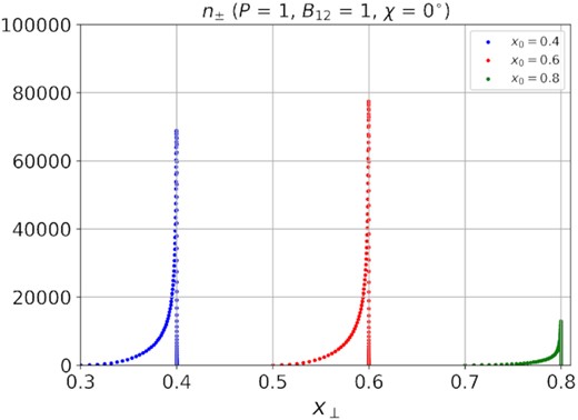
Secondary particle distribution n±(r⊥) (77) generated by a single primary particle with the starting points x0 = 0.4, x0 = 0.6, and x0 = 0.8 for P = 1 s, B12 = 1, and χ = 0°.
where

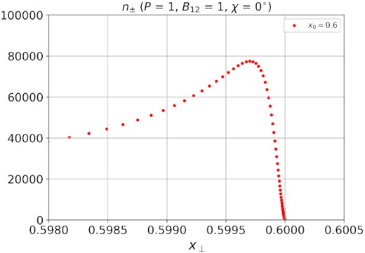
Secondary particle distribution n±(r⊥) (77) generated by a single primary particle with the starting points x0 = 0.6 near the threshold x⊥ = x0.
Finally, Table 4 shows how the multiplicity λ (i.e. the total number of secondary particles ne = n+ + n− per one primary particle) depends on the position r0 = x0R0. As one can see, taking into account the effects of general relativity leads to a significant (by several times) increase in the production rate of secondary particles. Therefore, it seems necessary to include the effects of general relativity in the consideration of the processes of the production of secondary particles near ‘the death line’.
Multiplicity λ for P = 1 s, B12 = 1, and χ = 30°.
| x0 | 0.1 | 0.2 | 0.3 | 0.4 | 0.5 | 0.6 | 0.7 | 0.8 | 0.9 |
| λ | 0 | 36 | 157 | 305 | 382 | 350 | 209 | 42 | 0 |
| λGR | 7 | 173 | 498 | 829 | 995 | 1040 | 663 | 220 | 3 |
| x0 | 0.1 | 0.2 | 0.3 | 0.4 | 0.5 | 0.6 | 0.7 | 0.8 | 0.9 |
| λ | 0 | 36 | 157 | 305 | 382 | 350 | 209 | 42 | 0 |
| λGR | 7 | 173 | 498 | 829 | 995 | 1040 | 663 | 220 | 3 |
In Fig. 4, we show the 2D distribution of the effective secondary particle multiplicity λ(x⊥) = (n+ + n−)/nprim (84) generated by the primary particles with the homogeneous distribution nprim = 1 for an ordinary pulsar (P = 1 s, B12 = 1, χ = 30°). The right shifted distribution corresponds to the multiplicity λGR(x0) presented in Table 4. The fitting curves for x⊥ ≪ 1 correspond to asymptotic behaviour |$n_{\pm } \propto x_{\perp }^3$| (see Andrianov et al., in preparation), which, as we see, are satisfied with good accuracy. As expected, the 2D distribution λ(x⊥) is shifted left relative to the distribution λGR(x0), since, as was shown in Fig. 2, secondary particles are born closer to the magnetic axis compared to the position of the primary particle (x⊥ < x0).

4.2 Inflow
Let us note straight away two essential circumstances. At first, for the formation of a particle production cascade, secondary electron–positron pairs corresponding to the most energetic γ-quanta must be produced in the region of a sufficiently strong longitudinal electric field E∥ so that one of the produced particles can stop and then be accelerated in the opposite direction (i.e. inwards to the star surface). For ordinary pulsars, this occurs at distances from the star’s surface h ≪ Rcap, where the very existence of a longitudinal electric field is beyond doubt (Ruderman & Sutherland 1975; Arons 1982).
However, near ‘the death line’, the free path length lγ of γ-quanta propagating outwards become much larger than the size of the polar cap. Therefore, secondary particles begin to be born at the distances from the star surface h ≫ Rcap where the longitudinal electric field, as was previously assumed, practically vanishes. However, as was shown, in a real dipole geometry, the longitudinal electric field also exists at large distances. It turns out that such an additional longitudinal field |$E_{\parallel }^{\rm add}$| (34) is sufficient to stop the particles at the distances h ∼ R from the star surface.
Here, however, one should pay attention to the fact that the additional longitudinal electric field |$E_{\parallel }^{\rm add}$| works effectively only on that part of the polar cap which is located closer to the rotation axis (sin φ > 0 for χ < 90° and sin φ < 0 for χ > 90°). In the other parts of the open field lines, where the opposite inequalities are made, the direction of the additional longitudinal electric field will be opposite to the electric field near the star surface. In particular, for sin φ = 0, there is no additional longitudinal electric field |$E_{\parallel }^{\rm add}$| at all.
Finally, we note one more circumstance which significantly distinguishes the processes of pair creation by γ-quanta moving towards the star compared to the case of moving from the star’s surface considered above. The point is that, as shown in Fig. 1, the particles moving from the surface of a star are accelerated on a scale R0 ≪ R, so that the free path length of γ-quanta can be comparable to the radius of the star. On the other hand, the particles moving towards the star gain most of the energy only near the very surface. Therefore, the free path length of γ-quanta should be of the order of R0.
Here x = h/R0,

and we again use standard definition (15) for the dimensionless polar cap area f*. If inequality (94) is violated, then the free path length lγ becomes greater than the height above the surface of the neutron star h at which it was generated. In this case, γ-quantum does not have time to give birth to a pair before it collides with the surface.
5 DISCUSSION
Thus, in this Paper I, the first step was taken in a consistent analysis of the conditions leading to the cessation of the secondary pair production for a sufficiently large rotation period P (which, in turn, leads to the termination of radio emission). As is well known, in reality, we have not ‘the death line’, but ‘the death valley’ on the |$P-{\dot{P}}$| diagram, which, apparently, is related to the tail of the distribution on some physical parameters. What parameters determine this band will be the subject of Paper II.
As for Paper I, we started from our main assumption that near ‘the death line’, the polar regions are almost completely free of plasma. This made it possible to accurately determine the potential drop in the area of open field lines. In particular, it was shown that in a dipole magnetic field in the region of open field lines, there is a longitudinal electric field which can stop secondary particles even at sufficiently large distances h ∼ R from the surface of the star. To date, this property has not been known.
In addition, the corrections related to the effects of general relativity were determined. As expected, they turned out to be at the level of 10–20 per cent, i.e. at the same level of uncertainty which can be assumed in other quantities, such as the radius and moment of inertia of a neutron star. Nevertheless, due to the strong dependence of the production rate on the energy of primary particles, taking into account the effects of general relativity leads to a significant (several times) increase in the multiplicity of particle production λ. Therefore, in this work, they were included into consideration. Looking into the future, we immediately note that it can be expected that the spread in such quantities as the radius of the star R and the size of the polar cap R0 (and, certainly, the curvature radius of magnetic field lines Rc) should also lead to a noticeable expansion of ‘the death line’. Paper II will be devoted to the analysis of all these issues.
Further, the question of the spatial distribution of the secondary particles produced by curvature photons was investigated in detail (as to synchrotron photons, we assume that near ‘the death line’, they are not efficient in the production of secondary pairs). First of all, it was shown that a certain role in the production of secondary plasma can play γ-quanta, the energy of which is several times higher than the energy of the maximum of the spectrum 0.44(ℏc/Rc)γ3. This effect becomes especially important for the curvature γ-quanta propagating towards the neutron star surface. As a result, conditions (98) for the termination of the cascade were formulated quantitatively. A detailed analysis of the dependence of ‘the death line’ both on the parameters of a neutron star and on the possible existence of a non-dipole magnetic field is to be carried out in Paper II.
ACKNOWLEDGEMENTS
Authors thank Ya.N.Istomin and A.A.Philippov for useful discussions. This work was partially supported by Russian Foundation for Basic Research (RFBR), grant 20-02-00469.
DATA AVAILABILITY
The data underlying this work will be shared on reasonable request to the corresponding author.
Footnotes
This expression can be easily obtained from a well-known synchrotron spectrum (Landau & Lifshits 1971) by replacing the Larmor radius rL = mec2γ/eB with the curvature radius of the magnetic field line Rc.
When |${\cal B} = 0.05$|, we have a single root at |$h = 0.13\, R_{0}$|.
REFERENCES
APPENDIX A: APPROXIMATION BY BESSEL FUNCTIONS


Finally, in Fig. A3, we present the comparison of the dimensionless parallel component of the electric field E∥ = −(∇ψB)/B/(ψ0/R0) calculated for cylindrical and conical geometries for P = 1 s, B12 = 1, and χ = 0°. As we can see, although in the first case, the expansion is carried out in exponential functions |$e^{-\lambda _{i}z}$|, and for dipole geometry in power-law dependencies |$(r/R)^{-\lambda _{i}/\theta _{0}}$|, their difference becomes indistinguishable already for four first terms of the series. Moreover, good enough agreement is achieved using only the first exponential term (dash line). In turn, this confirms the possibility to write down the condition for the presence of a cascade of secondary plasma production (i.e. the condition that secondary particles will be produced both for primary particles accelerated from the stellar surface and for the opposite motion) as (107).

