


ABSTRACT
Type Ia supernovae (SNe Ia) in the nearby Hubble flow are excellent distance indicators in cosmology. The Zwicky Transient Facility (ZTF) has observed a large sample of SNe from an untargeted, rolling survey, reaching 20.8, 20.6, and 20.3 mag in g r, and i band, respectively. With an FoV of 47 deg2, ZTF discovered > 3000 SNe Ia in a little over 2.5 yr. Here, we report on the sample of 761 spectroscopically classified SNe Ia from the first year of operations (DR1). The sample has a median redshift |$\bar{z} =$| 0.057, nearly a factor of 2 higher than the current low-z sample. Our sample has a total of 934 spectra, of which 632 were obtained with the robotic SEDm on Palomar P60. We assess the potential for precision cosmology for a total of 305 SNe with redshifts from host galaxy spectra. The sample is already comparable in size to the entire combined literature low-z anchor sample. The median first detection is 13.5 d before maximum light, about 10 d earlier than the median in the literature. Furthermore, six SNe from our sample are at DL < 80 Mpc, for which host galaxy distances can be obtained in the JAMES WEBB SPACE TELESCOPE era, such that we have calibrator and Hubble flow SNe observed with the same instrument. In the entire duration of ZTF-I, we have observed nearly 50 SNe for which we can obtain calibrator distances, key for per cent level distance scale measurements.
1 INTRODUCTION
In the two decades since the discovery of the accelerated expansion of the universe (Riess et al. 1998; Perlmutter et al. 1999), thought to be driven by the as yet poorly understood ‘dark energy’ component (see Goobar & Leibundgut 2011, for a review), Type Ia supernovae (SNe Ia) have been developed to become mature cosmological probes (Betoule et al. 2014; Scolnic et al. 2018; Brout et al. 2019). Despite the progress in SN Ia observations, the nature of the underlying physical mechanism driving acceleration remains an open question, with several potential explanations (see e.g. Dhawan et al. 2017; Lonappan et al. 2018). Increasing sample sizes of SNe Ia decreases statistical errors; hence, improving our understanding of dark energy relies on similarly reducing systematic uncertainties. Recent studies find that the systematic and statistical uncertainties on the measurement of the dark energy equation of state, w, are approximately equal (Conley et al. 2011; Scolnic et al. 2018; Brout et al. 2019; Jones et al. 2019). Apart from measuring dark energy properties, SNe Ia in the nearby Hubble flow, i.e. redshift range z ≲ 0.1 (hereafter also referred to as ‘low-z’) are also critical for measuring the present-day expansion rate, i.e. the Hubble constant (H0) precisely. Over the last decade, several improvements in the measurements of H0 (Riess et al. 2019) have revealed a >4σ tension between the local measurement of H0 based on Cepheid calibrated SNe Ia and the value inferred from the early universe (Planck Collaboration VI 2018).
This discrepancy could be an indicator of novel cosmological physics, e.g. early dark energy, additional relativistic neutrino species (present a summary of possible explanations Knox & Millea 2020). However, the tension could be caused by poorly understood astrophysical systematics (see, e.g. Scolnic et al. 2019; Freedman 2021; Mortsell et al. 2021a,b). There is significant debate regarding the impact of SN Ia environments and host galaxy properties on the inferred SN Ia luminosity, and hence, H0 (Rigault et al. 2015; Jones et al. 2018; Rigault et al. 2020). Conclusively testing the extent of the bias on H0 requires probing the underlying distribution of SN Ia host galaxy properties, which is not possible with observing campaigns targeted to specific host galaxy types. Having a sample of SNe Ia discovered and followed up by the same, untargeted survey is, therefore, crucial to observe the entire range of SN Ia environmental properties and test for possible biases in inferring cosmological parameters.
Dark energy inference with SNe Ia relies on relative distances. The high-z SNe Ia magnitude–redshift relation needs to be ‘anchored’ at low-z. The current low-z anchor sample is compiled heterogeneously from several different photometric systems, each with its own set of systematic uncertainties, which can be correlated in a way that is extremely difficult to predict. Some of the surveys in the low-z anchor sample targeted pre-selected galaxies (e.g. the Lick Observatory Supernova Survey; Filippenko et al. 2001) and their sample selection and follow-up criteria are heterogeneous and sometimes not well documented. This leads to several systematic uncertainties relating to observational and selection biases. SN Ia samples at high redshifts (z ≳ 0.1) e.g. from Sloan Digital Sky Survey (SDSS; Kessler et al. 2009), Supernova Legacy Survey (SNLS; Conley et al. 2011; Sullivan et al. 2011), Panoramic Survey Telescope and Rapid Response System (Pan-STARRS; Rest et al. 2014; Jones et al. 2019) and Dark Energy Survey (DES; Brout et al. 2019), however, are homogeneously observed on single photometric systems. Hence, the low-z sample, counter-intuitively, contributes most significantly to the systematics error budget for dark energy inference from SNe Ia (see also Foley et al. 2018). Beyond their use as probes of the expansion history, SNe Ia have previously been used as tracers of local large-scale structure (LSS), e.g. for measuring bulk flows (Feindt et al. 2013; Mathews et al. 2016), the product of the growth rate and amplitude of mass fluctuation, i.e. fσ8 (Huterer et al. 2017). SNe Ia are significantly more precise distance indicators compared to methods using galaxy distance, e.g. the Tully–Fisher relation, (Kourkchi et al. 2020), and are, therefore, an exciting route to infer properties of local LSS. So far, SNe Ia samples have been very sparse, which is the largest limitation of current data sets for precision constraints on local LSS with SNe Ia.
The advent of modern, wide-field surveys has greatly increased the SN discovery rate almost by an order of magnitude (see, e.g. Shappee et al. 2014; Tonry et al. 2018; Graham et al. 2019; Jones et al. 2021), making it possible to overcome the aforementioned uncertainties. The Zwicky Transient Facility (ZTF), using the 48-inch telescope at Palomar, is the widest field transient survey in the optical for SN discovery and follow-up. ZTF, in phase-I of operations (hereafter ZTF-I) scanned the entire Northern night sky in the g, r filters, reaching ∼20.5 mag/pointing (Bellm et al. 2019a,b; Graham et al. 2019; Dekany et al. 2020), with a 3-d cadence. To create a definitive data set of low-z SNe Ia distances, the main survey was complemented by ZTF partnership surveys, including observations of a large fraction of the sky in the i-band. The ZTF SN Ia survey discovers and provides well-sampled light curves, for a large sample of spectroscopically classified SNe Ia in the z ≲ 0.1 range. This large sample of well-characterized SN Ia light curves from a single, rolling untargeted survey allows for a unique control of the systematics from photometric calibration, observational and astrophysical bias in SN cosmology. This is critical for overcoming the systematics in H0 and dark energy studies. Moreover, the large statistics and uniform sky coverage will help overcome existing uncertainties in inferring the growth of structure from SNe Ia (see e.g. Graziani et al. 2020).
In this paper, we present the data set from the first year of operations and first results from the ZTF SN Ia survey. The ZTF SNe Ia sample aims to (1) anchor current and future high-z SN Ia sample for dark energy studies, (2) unlock the study of LSS in the nearby universe, and (3) measure H0 using a unique, self-consistent, calibrator and Hubble-flow sample. With the anticipated deluge of well-observed high-z SNe Ia from the Vera Rubin Observatory Legacy Survey of Space and time (see The LSST Dark Energy Science Collaboration et al. 2018, for the science requirements document), the large, homogeneously measured, untargeted low-z sample of SNe Ia from ZTF has the potential to be a definitive data set for cosmology in the coming decade.
This paper is structured as follows. In Section 2, we describe the survey strategy, data set, and processing methodology. In Section 3, we describe the analysis and results from the first data release. We present a discussion and our conclusions in Section 4.
2 SURVEY, DATA SET, AND METHODOLOGY
The survey design and science objectives for ZTF are described in detail in Bellm et al. (2019a,b) and Graham et al. (2019). In this section, we summarize the aspects of the survey relevant for the SN Ia first data release (hereafter DR1) sample. This includes the extragalactic partnership survey, the selection and classification for our sample, association of the host galaxy and the source of the spectroscopic redshift. We also describe the pipeline used for obtaining multiband photometry for the SNe.
2.1 Survey strategy
ZTF uses a 47 deg2 field with a 600 megapixel camera to scan the entire northern visible sky at rates of ∼3760 deg2 per hour (Bellm et al. 2019a). This is more than an order of magnitude improvement in survey speed relative to its predecessor survey the Palomar Transient Factory (Rau et al. 2009). ZTF reaches 5σ depth of ∼ 20.8 mag in g and ∼ 20.6 mag in r band (AB mag) in 30-s exposures. The median seeing for the survey is 2.17, 2.01, and 1.82 arcsec in the g, r, and i bands, respectively.
ZTF, in phase-I of observations from 2018 March to 2020 November, operated a unique survey strategy with 40|${{\ \rm per\ cent}}$| of its time for public surveys financed by the American’s National Science Foundation as part of its Mid-scale Innovations Program (MSIP), 40|${{\ \rm per\ cent}}$| for partnership observations and 20|${{\ \rm per\ cent}}$| for Caltech programs. In this paper, we focus on the first year of observations, hence, unless mentioned otherwise, we refer to ZTF phase-I as ZTF. The SN Ia cosmology program derives its data set from a combination of public and partnership observations. During its MSIP time, ZTF observed the entire visible sky from Palomar in g and r filters every three nights with a fiducial exposure time of 30 s (Fremling et al. 2020). The distribution of the SNe across the sky is shown in Fig. 1, which also presents a graphical overview of the DR1 survey, including light-curve and spectral sampling. Crucially for studies pertaining to the measurement of local LSS, the SNe are distributed all across the sky (e.g. Feindt et al. 2013; Graziani et al. 2020).
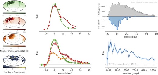
Left-hand panel: the number of observations during the first year of operations in the g (green), r (red), and i (orange) filters. The number of SNe Ia in each ZTF field are shown on the ZTF field grid in the bottom panel. Middle panel: an example light curve of an SN Ia at z ∼ 0.07 and ∼ 0.03 to show the typical sampling of the light curves in our sample. Right-hand panel: a histogram number of SNe with at least one light-curve point (top panel) and spectra (bottom panel) in each phase bin along with an example of the spectrum at z ∼ 0.033.
2.2 The partnership survey
The MSIP survey is complemented with ZTF partnership surveys. As part of these surveys, high-cadence data were obtained in the g and r bands as well as a wide-area i-band survey (Bellm et al. 2019b; Graham et al. 2019). The high-cadence survey, in the first year of operations, observed a total of ∼2500 deg 2 with three visits per night in the g and r bands, aimed at finding SNe in their infancy. This survey has been critical for early discoveries of SNe Ia (Yao et al. 2019), to characterize their rise times (Miller et al. 2020) and use the early colours as a test for explosion models and multiple populations (Bulla et al. 2020). The survey also provides densely sampled light curves in the g and r bands for the sample presented here.
The i-band survey involves 30-s-long exposures with a 4-d cadence, over a footprint of 6700 deg2, approximately one-quarter of the sky area of the MSIP survey, to a median nightly depth of 20.3 mag. The three filter photometry allows us to improve the constraints on the measured colour and is crucial to quantify colour calibration systematics. Previous studies extending the SN Ia Hubble diagram in the rest-frame i band to high-z (z ∼ 0.5 and higher) find a reduced contribution of systematics errors compared to the optical and argue for independent distances in the i band to the same SN Ia (Nobili et al. 2005; Freedman et al. 2009). At low redshifts, observations of SNe Ia in the iband have also been used to precisely estimate H0 (Burns et al. 2018).
SNe Ia show a diverse morphology at late times in the redder wavelengths (izYJHK filters). In the i band, the SNe rebrighten ∼2 weeks after the first peak, showing a characteristic second maximum, which is also an important diagnostic for SN Ia explosion properties (Hamuy et al. 1996; Folatelli et al. 2010). The double-peaked behaviour over the timescales of a few weeks makes them distinguishable from other SN types. In future photometric SN Ia surveys, having i band and redder coverage will be crucial to improve photometric classification. The ZTF gri data set is, therefore, an ideal testbed for such classification algorithms. Moreover, the second maximum in the near-infrared (NIR), has also been proposed as an alternate metric for standardization (Shariff et al. 2016). Hence, observations in the i band have several advantages for SN cosmology and will be a unique test of systematic errors.
2.3 Spectroscopy and sample selection
In this study, we focus on the sample of spectroscopically classified SNe Ia discovered in 2018, i.e. the first year of operations for ZTF. To include SNe Ia that were first detected in 2018 but continued to rise after the end of the year, we conservatively take SNe Ia that peaked before 2019 February 1. This compilation, hereafter known as the DR1 sample, consists of a total of 761 spectroscopically classified SNe Ia. These SNe Ia are on 340 unique ZTF fields corresponding to ∼2.2 SNe per field. Accounting for downtime in the survey operations during the first year, which corresponds to ∼2.5 SNe per field per year.
A summary of the first year of operations in presented in Fig. 1. In the left-hand panels, the ZTF field grid shows the number of g- (green), r- (red), and i- (orange) band observations along with the number of SNe per field.The extragalactic fields with a large number of g and r observations correspond to the high-cadence survey described in Section 2.2. We show an example light curve of an SN Ia with only MSIP and one with MSIP and partnership data to illustrate the typical sampling in the three filters. We show a histogram distribution of the number of SNe with at least one observation for each phase with a 1-d bin size. We find a significant fraction of SNe Ia have at least one observations before −7 d.
A large fraction of these SNe Ia were classified using the SEDmachine (Ben-Ami et al. 2012; Blagorodnova et al. 2018; Rigault et al. 2019), a low-resolution (R ∼100) integral field unit (IFU) spectrograph on the robotic Palomar 60-arcsec telescope (Cenko et al. 2006) as part of the ZTF Bright Transient Survey (BTS), with the goal to spectroscopically classify and publicly report every extragalactic transient in the Northern sky with r < 18.5 mag discovered by the ZTF public surveys. The SEDm is capable of classifying >10 SNe (of any type) per night in the 18.5–19 mag range. Details of the BTS program can be found in Fremling et al. (2020) and Perley et al. (2020). The data are reduced uniformly and consistently as part of the automated pysedm pipeline (Rigault et al. 2019).
For the complete sample of 761 objects, we have obtained a total of 934 spectra, hosted on the GROWTH marshal (Kasliwal et al. 2019). Out of the total, 632 spectra are obtained with the SED machine, which corresponds to |$\sim 68{{\ \rm per\ cent}}$| of the total sample of spectra. We present a distribution of the phase at which the spectra were obtained in Fig. 1 (top right-hand panel). A example of a high S/N spectrum for an SN at z = 0.0335 in shown in the bottom right-hand panel of Fig. 1.
2.4 Host galaxy redshifts
In our study, we want to infer the light-curve parameters for the SNe Ia in the DR1 sample (see Table 1 for a brief summary) and quantify the scatter in the Hubble residuals. This requires a robust, spectroscopic determination of the redshift to the SN host galaxy. We compile the SN Ia host galaxy redshifts here. A large fraction of these host galaxy redshifts are obtained from the Sloan Digital Sky Survey (SDSS) 16th data release (Ahumada et al. 2020). For SNe Ia that do not have a redshift for the host galaxy in SDSS, we obtain the redshift from the NASA Extragalactic Database (NED).1 In addition to host galaxy redshift constraints, we restrict the sample to SNe with sufficient data around and before maximum light from the alert pipeline. This is required to have a robust initial estimate of the time of maximum for creating custom reference and difference images to perform forced photometry (see Section 2.5 for details). The final sample with these constraints has 305 SNe Ia. The coordinates and redshifts for SNe Ia in this sample are presented in Table 2. Hereafter, we refer to this as the host-z sample.
The SNe Ia in the complete Year 1 sample along with their coordinates, classification, first observation date, instrument from which the spectrum has been obtained, approximate resolution of the instrument, and date of first spectroscopic observation.
| Name | IAU name | RA (°) | Dec. (°) | Classification | Obs date | Instrument | Resolution | Date of spectrum |
|---|---|---|---|---|---|---|---|---|
| ZTF18aaadqua | SN2018lq | 26.7987 | 18.7986 | SN Ia | 2018-1-14 | P200 | 100–10 000 | 2018-01-22 |
| ZTF18aabasml | SN2018tz | 166.486 4679 | 37.625 1311 | SN Ia | 2018-2-9 | P60 | 100 | 2018-02-21 |
| ZTF18aabqgnb | SN2018yc | 178.189 5182 | 37.854 2631 | SN Ia | 2018-2-9 | Lijiang2.4m | 300 | 2018-02-28 |
| ZTF18aabssme | SN2018aca | 155.711 5261 | 14.054 786 | SN Ia | 2018-3-5 | P60 | 100 | 2018-03-07 |
| ZTF18aabstmw | SN2018aaz | 153.451 1418 | 38.763 0928 | SN Ia 91bg-like | 2018-3-5 | P60 | 100 | 2018-03-07 |
Note. This table has been truncated to improve the presentation; the table in its entirety is available online.
SN names, heliocentric frame redshift, and coordinates (in degrees) for the SNe Ia in our sample.
| SN Name | zhelio | RA | Dec. |
|---|---|---|---|
| (°) | (°) | ||
| ZTF18aabdgik | 0.021 604 | 175.5987 | 10.2641 |
| ZTF18aabstmw | 0.023 086 48 | 153.4511 | 38.7631 |
| ZTF18aabsyqp | 0.076 672 08 | 162.8185 | 22.4776 |
| ZTF18aabtaor | 0.079 834 81 | 172.0952 | 44.7490 |
| ZTF18aabxrjp | 0.079 177 14 | 185.5432 | 26.9946 |
Notes. The table has been truncated for formatting reasons. Full table is available online.
We emphasize that while this criterion selects less than half (|$\sim 40{{\ \rm per\ cent}}$|) the total sample of SNe Ia (consistent with the findings of BTS Fremling et al. 2020), host galaxy redshifts are not time critical. These can be obtained after the completion of the survey. Several surveys using multiobject spectrographs e.g. the Dark Energy Spectroscopic Instrument (DESI; DESI Collaboration et al. 2016) and/or the 4MOST consortium extragalactic surveys (de Jong et al. 2019; Swann et al. 2019) can obtain spectra for galaxies that hosted ZTF observed SNe Ia, from which redshifts can be derived. Despite the incompleteness of available host redshifts, we note that even the host-z sample is larger than the entire, combined low-z anchor in current SN cosmology studies (e.g. Scolnic et al. 2018).
Our sample presented here has a median redshift of 0.057, which is nearly twice that of the median for the sample in the literature. Hence, the inferred cosmological parameters from this sample will be less prone to systematic errors from peculiar velocity corrections (see, e.g. Huterer 2020). The resulting redshift distribution for our sample is shown in Fig. 2. For the complete sample as well as the host-z only sample, we can see that median redshift is approximately twice the median of the current literature low-z sample (with All ZTF Y1 having a higher median z of 0.069).
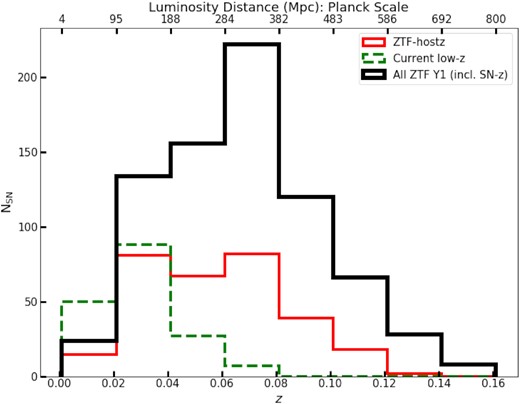
Histogram distribution of the redshifts from the DR1 sample with host galaxy redshifts (red) and the total sample with redshifts from any source, including fitting the SNID template to the SN spectrum (black) compared to the current low-z sample in the literature (green). The redshift distribution of our DR1 sample has a median z = 0.057, which is approximately twice higher than the median from the literature sample, hence making this sample significantly less sensitive to the uncertainties from peculiar velocity corrections.
2.5 Photometry pipeline
In this section, we describe the pipeline used for generating the photometry for our sample of SNe Ia. Since we want to measure light-curve model parameters and Hubble residuals, we focus on the host-z sample. While this is a custom-based pipeline for creating reference images, image subtraction, and source photometry, it uses certain aspects for the ZTF data products made available by the Image Processing and Analysis Center (IPAC) at Caltech; hence, we summarize those aspects here. The ZTF data processing, products, and archive are described in detail in Masci et al. (2019). IPAC provides alert packets with photometry as well as a forced photometry service at a pre-determined locations. We note that for a substantial fraction of the DR1 sample, building of reference images began during the survey operations and hence, overlapped in time with the discovery of astrophysical transients. Therefore, the alert and IPAC forced photometry for several SNe Ia had contamination from the live transient in the reference image. This required a reprocessing of the data to make customized references for the regions of the sky where the SNe Ia were discovered.
We use a state-of-the-art image processing pipeline, written using well-tested and widely used astronomical image processing tools for processing data from the ZTF Uniform Depth Survey (ZUDS).2 While the pipeline was designed for discovering slowly evolving faint transients on deep coadds of science frames, its versatile functionality makes it ideal for creating image subtractions and computing light curves using single exposures. Details of the individual components of the pipeline are presented in Appendix A. We summarize the pipeline features in this section.
Using the ZUDS pipeline, we create references for each ZTF field and CCD in which an SN Ia in our sample has been observed (see section 3 of Masci et al. 2019, for details about the ZTF CCDs). They are generated using the swarp (Bertin et al. 2002) software for coaddition. The associated reference mask is created with the mask images provided for each exposure by IPAC, using a bitwise logical AND (see Appendix A). When sufficient number of exposures are available, reference images are created by coadding epochs from before the SN explodes (which we determine as epochs 30 or more days before the time of maximum inferred from photometry provided by IPAC). For making the reference image, we only use images that were obtained in seeing conditions between 1.7 and 3 arcsec and have a deeper magnitude limit than 19.2 mag. If there are insufficient number of exposures (<20) for which the nightly conditions do not meet these criteria, the pre-SN exposures were combined with post-explosion images from >400 d after the time of maximum inferred from the alert photometry.
We generate difference images using the hotpants image subtraction software (Becker 2015). The subtraction is normalized to the science image and convolved to the template image. Details of the convolution kernel, half-width substamp, and the setup for the hotpants subtractions are described in Appendix A.
We use the photutilsastropy package (Bradley et al. 2019) for performing aperture photometry at the SN position, determined from the alert photometry provided by IPAC. For each epoch, the zero-point is derived from a combination of the nightly zero-point and aperture correction provided by IPAC (see Masci et al. 2019, for details).
3 ANALYSIS AND RESULTS
We analyse the host-z sample in this section, describe the spectroscopic properties and the sample demographics, in comparison with the literature sample. We also present the sample of SNe Ia that are at feasible distances to build a calibrator sample for local H0 measurements.
3.1 Light-curve fitting
To be used for cosmology, SNe Ia need to be standardized, using relations between their luminosity and the light-curve shape and colour, for measuring accurate distances (see Leibundgut & Sullivan 2018, for a review of how SNe Ia are used in cosmology). Here we describe the procedure for fitting the light curves generated using the pipeline described in Section 2.5, to derive the peak apparent brightness, light-curve width, and colour.
There are several algorithms in the literature to estimate distances from SN light curves, e.g. MLCS (Jha, Riess & Kirshner 2007), SiFTO (Conley et al. 2008), BayeSN (Mandel et al. 2009; Mandel, Narayan & Kirshner 2011; Mandel et al. 2020), SNooPy (Burns et al. 2011), and BaSALT (Scolnic et al. 2014). Each light-curve fitting method makes a correction to the SN luminosity for the light-curve shape and colour. The colour correction, however, can be applied in two principly different ways. The first uses an empirical correlation between the observed colour and the uncorrected Hubble residuals, whereas the second assumes that the observed colour is a combination of intrinsic SN colour, photometric errors, and reddening due to dust, e.g. in the SN Ia host galaxy. The former is more model independent, whereas the latter is more physically motivated. In-depth comparisons of different light-curve fitters in the literature (e.g. Kessler et al. 2009) find that, in general, they agree reasonably well given the same input assumptions.
Currently, the most widely used light-curve fitting algorithm is the Spectral Adaptive Lightcurve Template – 2 (SALT2; Guy et al. 2007), based on the SALT method (Guy et al. 2005) and we use this in our analysis. The SALT2 model treats the colour entirely empirically and is used to find a global colour–luminosity relation. We use the most updated, published version of SALT2 (SALT2.4; see Guy et al. 2010) as implemented in sncosmo v2.1.03 (Barbary et al. 2016). In the fitting procedure, we correct the SN fluxes for extinction due to dust in the Milky Way (MW). We use extinction values for the SN coordinates (presented in Table 2) derived in Schlafly & Finkbeiner (2011). These are updated galactic extinction maps that find that the extinction values from Schlegel, Finkbeiner & Davis (1998) were overestimated. We use the widely applied galactic reddening law, proposed in Cardelli, Clayton & Mathis (1989), known as the ‘CCM’ law to correct for MW extinction. For the extinction corrections, we use the canonical value for the total-to-selective absorption, RV = 3.1.
We fit the SALT2 model to each SN Ia in two steps. First, we fit without the SALT2 model covariance to obtain an initial guess for the time of maximum, t0. We select the data in the phase range −20 to + 50 d relative to the initial guess t0, corresponding to the phase range in which the SALT2 model is defined. For the fit, we use an error floor of 2|${{\ \rm per\ cent}}$| of the flux, corresponding to the the typical photometric calibration accuracy with respect to Pan-STARRS1 reported in Masci et al. (2019). We note that this is appropriate since we use the zero-point report by IPAC in Masci et al. (2019) for fitting the fluxes computed from the photometry.
We then fit the data only in this phase range along with the model covariance to get the final fit parameters. The resulting parameters are reported in Table 3. As we can see in Fig. 3, ZTF18aaumeys, shown as an illustrative example SN, has a significant number of detections on the rising part of the light curve. This can be used to improve the standardization relative to just the standard stretch and colour corrections (as in equation 1), and ultimately reduce the intrinsic dispersion in the sample. It has been proposed in the literature that separating the light-curve width parameter x1, into an x1 from the rising and falling parts of the light curve, |$x_1^r$| (labelled as the rising width in Fig. 3) and |$x_1^f$|, can improve the light-curve fit. Since it has been shown that for a given decline rate, the rise times vary significantly (Ganeshalingam, Li & Filippenko 2011; Firth et al. 2015; Miller et al. 2020), we expect to gain in the precision of the distance measurement by using information in rising part of the light curve. It has been shown that this method of two light-curve widths instead of one yields a smaller scatter than if only using a single light-curve width (Hayden, Rubin & Strovink 2019). ZTF18aaumeys is also an example SNe Ia that has data extending beyond the range of phases for which the SALT2 model is valid, which makes it interesting to use this data for further extending the SALT2 model beyond the phase range of + 50 d. The data set presented here allows us to test these novel standardization procedures in the future.
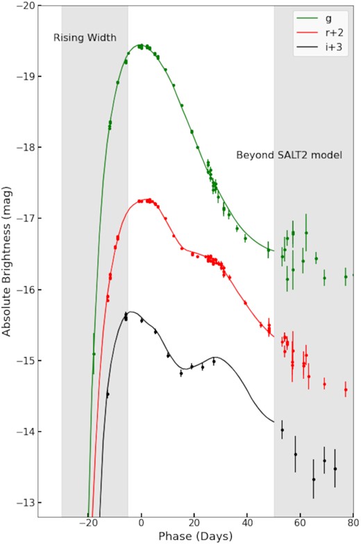
An example of fitting the SALT2 model to ZTF18aaumeys, as implemented in sncosmo. The SN is at redshift 0.033, well into the Hubble flow and the light curve is sampled extremely well on the rising part, which also allows us to explore beyond the conventional standardization parameters. Data for this SN extend beyond + 50 d, the validity limit of the SALT2 model. Hence, we can use SNe in our sample to retrain the SALT2 model and extend to later phases. We note here that the SALT2 model has only been fitted to the g- and r-band data, whereas for the i band, only the predicted model light curve is overplotted on the data.
Output SALT2 fit parameters for SNe in our sample along with the CMB frame redshift (zCMB; see the text for the CMB frame conversion).
| ZTF Name | zCMB | mB | x1 | c |
|---|---|---|---|---|
| (mag) | ||||
| ZTF18aabdgik | 0.022 775 296 | 15.516 (± 0.047) | 0.096 (± 0.218) | 0.034 (± 0.038) |
| ZTF18aabstmw | 0.023 919 309 | 18.005 (±0.066) | −1.302 (±0.148) | 0.433 (±0.048) |
| ZTF18aabsyqp | 0.077 744 924 | 18.579 (±0.121) | 0.556 (±0.221) | 0.193 (±0.091) |
| ZTF18aabtaor | 0.080 5990 43 | 18.397 (±0.075) | 0.659 (±0.451) | −0.045 (±0.057) |
| ZTF18aabxrjp | 0.0801 525 26 | 18.479 (±0.070) | −0.732 (±0.433) | 0.022 (±0.053) |
Notes. We report the mB, x1 and c parameters used to compute the Hubble residuals (full table available online; fit outputs including covariances between the fit parameters are provided in the github repo).
3.2 The gri-sample
For the host-z sample, we have a total of 170 SNe Ia with at least one observation in the i band between −15 and + 15 d relative to the Tmax inferred from the SALT2 fits to the g- and r-band data. However, to get robust detections, we need deep references to create good difference images. Therefore, we further require at least 15 frames in the i band either the phase range before −30 d or after + 400 d to make the reference image. Hence, for the i band, we further impose the cut of the number of frames to create a reference image. We note that for our host-z sample, out of the 305 SNe, 122 have at least one detection in the i-band. This corresponds to |$\sim 40{{\ \rm per\ cent}}$| of the SNe in the sample, which is consistent with the predictions from Feindt et al. (2019). We emphasize that this is a lower limit, with the number expected to increase with an increase in the number of observations after the SN has faded, for making a reference image.
The light-curve fits for the SNe that peaked within 60 d since 2018 June 15 are shown in Fig. 4. We note that the fit is only to the g- and r-band data and the solid black lines in the bottom panel are the SALT2 model predictions in the i band overplotted on the data. The sample parameters are discussed in Section 3.4 along with further selection cuts in Table 4.
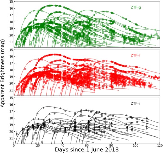
Light curves for the DR1 host-z sample in the g, r, i filters for SNe Ia that peak within two months of 2018 June 15 (shown as days from 2018 June 1). The SALT2 model fits to only the g- and r-band data are overplotted as solid lines.
Selection criteria for the DR1 sample. The initial sample in boldface is the entire DR1 SNe Ia independent of the source of redshift, hence, the first criterion is a redshift from the host galaxy. Ellipses signify no cut since its the initial sample..
| Criterion | |$\#$| of SNe | Cumulative |$\#$| of SNe | Remaining SNe |
|---|---|---|---|
| not passing | not passing | ||
| All DR1 | … | … | 761 |
| Host-z | 456 | 456 | 305 |
| Spectroscopically peculiar, | 11 | 467 | 294 |
| z ≥ 0.015, | 5 | 472 | 289 |
| z ≤ 0.1, | 23 | 495 | 266 |
| >3 points between −10 and + 10 d | 26 | 521 | 240 |
| σ(x1) < 1, σ(t0) < 1 | 11 | 532 | 229 |
| −3 < x1 < 3 | 2 | 534 | 227 |
| −0.3 < c < 0.3 | 25 | 559 | 202 |
| Chauvenet’s criterion (>4σ outlier) | 2 | 561 | 200 |
Notes. The final sample, after quality cuts is used to compute the Hubble residuals. The strongest cut is for an available host galaxy redshift, which are not time-critical.
3.3 Spectroscopic properties
The sample presented here is comprised entirely of spectroscopically classified SNe Ia. This is critical to remove contamination from core-collapse SNe and other non-SN Ia transients. Several studies in the literature have demonstrated that SNe Ia can be divided into subclasses based on spectral line velocities near maximum light, with potential implications for distance measurements (Wang et al. 2009; Foley & Kasen 2011; Folatelli et al. 2013; Siebert et al. 2020; Dettman et al. 2021). Therefore, having spectra is important for improving cosmological inference with SNe Ia. The phase distribution for the spectra of the SNe Ia in the host-z sample is shown in Fig. 5. We find no significant difference in the phase distribution of the spectra from all instruments and the SEDm alone. 50|${{\ \rm per\ cent}}$| of all spectra (and 50|${{\ \rm per\ cent}}$| of all SEDm spectra) are obtained before maximum light, while 23|${{\ \rm per\ cent}}$| (20|${{\ \rm per\ cent}}$| for SEDm) are obtained before −7 d. Here, measure the accuracy of the line velocities from spectra obtained with the SEDm.
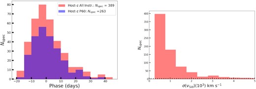
Left-hand panel: phase distribution of the spectra in the host-z sample from all instruments (red) and from SEDm alone (blue). Similar to the complete DR1 sample, |$68{{\ \rm per\ cent}}$| of all spectra are obtained using SEDm. Right-hand panel: the histogram distribution of the errors on the Si ii 6355 Å line velocity (in km s−1) from only the SEDm spectra for the SNe in our sample, inferred using the spextractor software. We find a median error of ∼700 km s−1.
Since we aim to measure the accuracy of line velocities, we require an independent determination of the redshift and hence, we use the host-z sample of 305 SNe Ia, which is a lower limit since the host redshift are not time critical (see section 2.4). In this analysis, we only focus on the ubiquitous Si ii 6355 Å feature, since the velocity of this feature has been most widely proposed in the literature as a metric for subclassifying SNe and improving distances. We reiterate that a large fraction (68 |${{\ \rm per\ cent}}$|) of the spectra for our sample are obtained with a single instrument, i.e. SEDmachine, extracted uniformly with the pysedm pipeline (Rigault et al. 2019).
For our line velocity measurements we use a fully automated and public code for spectral fitting, spextractor(Papadogiannakis 2019).4 The code uses a non-parametric, Gaussian process (GP) regression (Rasmussen & Williams 2005) to get the minima for the individual features. It is based on the publically available python package gpy (GPy 2012) and uses a Matern 3/2 kernel for smoothing the spectra.
The median error in the inferred vSi is ∼700 km s−1. We emphasize that this method has fewer model assumptions than methods used in the literature. Hence, we expect the median errors to be higher compared to e.g. a fit assuming multiple Gaussians describe the line profile. However, even with such precision on the velocity measurements, we can clearly distinguish high- and low-velocity subtypes to test improvements in the distance measurements with our sample. A detailed analysis of the method and the spectral sample, as well as relations with light curve and host galaxy parameters will be presented in a follow-up study (Johansson et al. in preparation).
3.4 Sample cuts and demographics
In this section, we describe quality cuts on the host-z sample. We perform cuts based on the SN Ia spectral subtyping, redshift range, and light-curve parameters to get the final sample with which to compute the Hubble residuals. We then compare the light-curve fit parameters and the Hubble residuals to the current low-z from the literature.
The first selection cut is to remove peculiar SNe from the final analyses. These include SNe Ia that are spectroscopically similar to the class of SNe Iax (Jha et al. 2006; Foley et al. 2013) the eponymous subluminous and fast-declining SN 1991bg (Filippenko et al. 1992; Leibundgut et al. 1993) or Ia-CSM, similar to the prototype SN 2002ic (Hamuy et al. 2003; Wood-Vasey, Wang & Aldering 2004). This is because such peculiar SNe might not follow the width–luminosity relation (Phillips 1993) or they may not be adequately described by the SALT2 model. However, we do not remove SNe Ia in the subclass similar to SN 1991T. This is for two reasons. Their peculiarities are shown to be almost exclusively spectroscopic, and they are shown to obey the width–luminosity relation (see Taubenberger 2017, for a discussion on the extremes of thermonuclear SNe). Furthermore, we note that 91bg-like objects might not be inherently incalibratable, since there are fitting algorithms other than SALT2, e.g. MLCS2k2 (Jha et al. 2007) with which it is possible that can estimate distances for this subclass of SNe Ia, however, for our current analyses, we remove them from the cosmological sample, but possibly might include them in the future (see also Foley et al. 2018 for cuts to the Foundation SN sample).
We apply cuts based on the redshift of the host galaxy. Since this sample is uniquely discovered, followed up, and characterized with a single telescope and instrument, we do not have an a priori truncation on the redshift range. We apply a lower limit on the redshift distribution of z ≥ 0.015, to minimize errors from peculiar velocity corrections, as done in previous studies in the literature (see e.g. Foley et al. 2018). The ZTF BTS reports a completeness of 97|${{\ \rm per\ cent}}$| at m < 18 mag and 93|${{\ \rm per\ cent}}$| m < 18.5 mag (Perley et al. 2020). The ZTF BTS is |$\gtrsim 70{{\ \rm per\ cent}}$| complete till m < 19 mag, corresponding to a z ≲ 0.1 threshold; hence, we apply an upper limit on the redshift of z ≤ 0.1.
In our analysis, we want to robustly determine the light-curve fit parameters, hence, we restrict the sample to SNe with at least three points in the light curve within 10 d of maximum light. Furthermore, we remove poor SALT fits, defined as having σ(x1) > 1 or σ(t0) > 1 d. For the final sample, we also remove SNe with extremely slow or fast declining light curves, i.e. |x1| > 3 and SNe with extremely blue or red colours, i.e. |c| > 0.3. We note that these SNe are of interest to SN Ia explosion physics, environmental properties, and reddening due to dust in the host galaxy (e.g. Bulla, Goobar & Dhawan 2018), but are removed when computing the Hubble residuals. Finally, we apply Chauvenet’s criterion on the sample. The selection cuts are summarized as follows:
Spectroscopically classified as a normal SN Ia, i.e. not spectroscopically similar to SNe Iax (Jha et al. 2006; Foley et al. 2013), SN 1991bg (Filippenko et al. 1992; Leibundgut et al. 1993), or Ia-CSM (Hamuy et al. 2003; Wood-Vasey et al. 2004).
0.015 ≤ z ≤ 0.1.
At least three points between −10 and + 10 d.
The uncertainty on x1 is <1.
−3 < x1 < 3.
−0.3 < c < 0.3.
Chauvenet’s criterion to exclude systematic outliers.
Here, we describe the objects in our sample removed with each of the above selection cuts. Our sample includes a total of 11 spectroscopically peculiar SNe Ia, 9 of which belong to the subclass of 91bg-likes, 1 Type Iax SN, and 1 SN Ia-CSM. For the 91bg-likes that have sufficient coverage between −10 and + 10 d, we derive the SALT2 light-curve parameters. For five of the seven SNe Ia, the SALT2 c > 0.3, consistent with the observation in the literature that 91bg-likes are redder than normal SNe Ia.
We remove 27 SNe that do not have enough observations near maximum light and 9 SNe that do not have an accurately measured x1. Only 2 SNe are outside the range of x1 values for cosmologically viable SNe Ia. We find 25 SNe with |c| > 0.3, 23 of which are reddened with a c > 0.3. We find more reddened SNe in our sample than in other low-z, cosmological samples in the literature. Additionally, even within the cosmological sample, there are more SNe Ia in the range 0.25 < c < 0.3 compared to the existing low-z. The larger number of high-c SNe could be due to the fact that our sample is derived from an untargeted survey, where we do not a priori reject reddened SNe when building a light curve, however, we will explore this in detail in future works. We finally apply Chauvenet’s criterion and find only two SNe removed with this cut, ZTF18ablqkud and ZTF18aarcypa. They have a δμ of 0.76 and 0.77 mag, respectively, making them both significantly fainter than the other SNe in the sample. While faint, ZTF18ablqkud does not show an spectroscopic features similar to the class of SN 1991bg-like SNe and has a broad r-band light curve, which is consistent with normal SN Ia. It has an inferred x1 = 0.88 ± 0.22 and c = 0.129 ± 0.034, which are also consistent with the values for normal SNe Ia. ZTF18aarcypa similarly does not show spectroscopic features similar to SN 1991bg, and it shows a shoulder in the r-band, however, it has a low x1 = −2.89 ± 0.29, which is consistent with the class of transitional fast decliners (Hsiao et al. 2015). A summary of the number of objects removed after each cut is presented in Table 4.
We compare the x1 and c distribution for our sample (top and middle panel in Fig. 6) with the low-z anchor sample for dark energy studies in the literature (Scolnic et al. 2018). Using a Kolmogorov–Smirnov test, we find a p-value of 0.03 and 0.6 for the x1 and c distribution. For the x1 parameter, we can tentatively reject the hypothesis that both distributions are drawn from the same parent population. We will investigate this in detail in future works. We cannot reject the null hypothesis that both c distributions come from the same parent population; however, we find a larger fraction of c > 0.3 SNe Ia in our sample compared to the low-z samples in the literature.
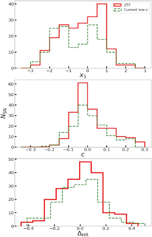
(Top panel) SALT2 light-curve width (x1), (middle panel) colour (c) parameters, and (bottom panel) the Hubble residuals computed after fitting the nuisance parameters for the ZTF DR1 sample (red, solid) compared to the low-z sample used for cosmological studies in the literature (green, dashed). We find that the x1-distributions for the ZTF and literature sample appear to be drawn from different parent populations; however, the c-distribution for the ZTF sample, within the |c| > 0.3 does not. We note, however, that the sample has a larger fraction of c > 0.3 SNe Ia compared to the literature (see Table 4) The σrms of the Hubble residuals is 0.17 mag, which is very similar to the σrms of the literature sample.
3.4.1 Host galaxy mass
Here we compute stellar masses (Mstellar) for the host galaxies of SNe Ia in our host-z sample. We take the host galaxy photometry from PanSTARRS legacy imaging (Chambers et al. 2016) and identify the host galaxy using the ‘Directional Light Radius’ (DLR; Sullivan et al. 2006; Smith et al. 2012) methodology, requiring DLR < 5. SNe with no host satistfying this criteria (5; 2 per cent) are considered hostless. Stellar masses are computed by comparing measured griz-band fluxes to those of spectral energy distribution (SED) model at the redshift of the SN. For this, we use the spectral synthesis code, PÉGASE2 (Fioc & Rocca-Volmerange 1997; Le Borgne & Rocca-Volmerange 2002) combined with a Kroupa (2001) initial mass function (IMF) to calculate synthetic SEDs. We consider nine exponentially declining star formation histories (SFHs) evaluated at 102 time-steps with SFR(t) = exp−t/τ/τ, where t is the age of the galaxy and τ is the e-folding time, each with seven foreground dust screens (see Smith et al. 2020, for more details). We present the Mstellar distribution for our sample in Fig. 7. For comparison, we also analyse the host galaxies of the current low-z sample with the same procedure. We find a slightly larger fraction of low (log |${M_{\rm stellar}}/{{\rm M}_{\odot }} \lt 10$|) mass hosts compared to the literature sample. However, we note that requiring a spectroscopic redshift from the literature could lead to some preference against fainter and even lower mass hosts in the host-z sample compared to the entire DR1 sample. Therefore, we also compute the masses for the entire DR1 sample. We find that compared to the 23.8|${{\ \rm per\ cent}}$| of SNe Ia in low-mass galaxies in the current low-z, the ZTF Y1 spec-z sample has 31.6|${{\ \rm per\ cent}}$| of the SNe Ia in low-mass galaxies and ZTF Y1 all-z has 48.1|${{\ \rm per\ cent}}$| of the SNe Ia in low-mass galaxies. A detailed analysis of the host galaxies of all SNe Ia in the DR1 sample will be presented in a follow-up study (Smith et al. in preparation). This furthermore emphasizes the need for post-survey SN Ia host spectroscopy to obtain redshifts.
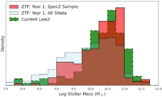
Log of the host stellar mass distribution for the DR1 host-z sample (red), DR1 all-z sample (i.e. including SNe where the redshift is determined from the SN spectrum itself) (blue), and the current low-z SN Ia sample (green). The Y1 sample has |$48.1 {{\ \rm per\ cent}}$| of all SNe Ia in low-mass host galaxies compared to 23.8|${{\ \rm per\ cent}}$| for the current low-z distribution.
3.4.2 Hubble residuals
For the sample after the selection cuts described above we derive the distribution of the Hubble residuals. From the fit to the magnitude–redshift relation, we derive the the rms (σrms) and intrinsic scatter (σint) values. The σint value is fitted simultaneously with the coefficient of the width–luminosity and colour–luminosity relations, which allows us to robustly infer σint, instead of fixing it to give an adequate goodness of fit.
While for the light-curve fitting we fix the SN model redshift to the heliocentric frame, for our inference of the Hubble residuals use CMB frame redshifts. We convert the heliocentric redshifts to CMB frame using the standard conversion formula and the dipole velocity and position of the CMB from Fixsen et al. (1996). Since we cannot constrain ΩM from low-z SNe Ia themselves, we fix it to the value from Planck of 0.307 (Planck Collaboration VI 2018).
The σpec magnitude error is derived assuming a stochastic peculiar velocity error value of 300 km s−1 (Carrick et al. 2015), and σint to account for the intrinsic scatter of the SNe Ia. Here, the σfit error term is derived from the output covariance matrix of the SALT2 model fit, for a given value of α and β. Hence, in our inference, we fit the magnitude–redshift relation with four free parameters, namely the intercept of the magnitude–redshift relation, α, β, σint with uninformative priors on each. We use pymultinest (Buchner et al. 2014), a python wrapper to multinest (Feroz, Hobson & Bridges 2009) to derive the posterior distribution on the parameters.
For the best-fitting parameter estimates, we obtain a σrms of 0.17 mag. We note that this is comparable to the light-curve scatter from other low-z samples in the literature, when analysed with the SALT2 model (see, e.g. Thorp et al. 2021) as well as low-z sample of SNe Ia used in cosmological studies (e.g. Scolnic et al. 2018). Moreover, if we do not apply the final selection cut of the Chauvenet criterion and keep the two SNe Ia that do not pass the cut in the sample, the σrms = 0.18 mag, hence, the rms scatter is not impacted significantly by the removal of outliers. A comparison of the Hubble residuals with the current low-z sample from the literature is shown in Fig. 6 (bottom panel). Our sample has a σint = 0.15 mag. We note that the rms dispersion and σint are higher than report values for high-z sample (e.g. Scolnic et al. 2018; Abbott et al. 2019) We emphasize that the intrinsic scatter term is not derived for a complete treatment of the systematic uncertainties, but rather only includes a statistical error term that is a combination of the fit error and the peculiar velocity error. We would expect the intrinsic scatter value to be lower when including a complete systematics uncertainty budget.
We emphasize that since there are ongoing improvement to the data processing pipeline, the inferred root mean square (rms) and intrinsic scatter values should be considered as preliminary upper limits, expected to improve in subsequent analyses. We caution against using the reported fit values for inferring cosmological parameters and conducting more detailed cosmological analyses, e.g. for H0 or dark energy properties We have not yet produced a complete systematics error budget. Therefore, at this stage in our analyses we are blind to the parameters governing the width–luminosity and colour–luminosity relations as well as the intercept of the Hubble diagram till such a complete systematics analysis has been performed.
3.5 Potential calibrator sample SNe Ia
In the sections above, we have focused on the SNe Ia at higher redshift in our sample. While the lowest redshift SNe in our data set cannot be used for the Hubble flow rung of the distance ladder, with future ground- and spaced-based observatories, we can expect measurements of independent, calibrated distances to their host galaxies, using secondary distance indicators. This would be possible to distances of DL ∼ 80 Mpc or approximately translating to z ∼ 0.02 (see, e.g. Beaton et al. 2019). Such measurements in the literature use Cepheid variables (Riess et al. 2019), TRGB stars (Freedman et al. 2019), JAGB stars (for e.g. Freedman & Madore 2020; Lee et al. 2020), or Mira variables (Huang et al. 2020).
The large uncertainty from heterogeneously calibrated instruments and photometric systems also impacts the local H0 measurement via the calibrator sample of SNe Ia. Hence, the ZTF sample offers a unique opportunity to have a homogeneously observed calibrator sample of SNe Ia, on the same instrument as the Hubble flow SNe Ia.
In our sample, we have 14 SNe at z < 0.02. When applying the criteria for the final sample selection as in Section 3.4, we find that six SNe pass the cuts. Of the SNe rejected by the cuts, there is one spectroscopically peculiar (91bg-like), three have high reddening (c > 0.3) and four do not have sufficient sampling near peak. We emphasize that these six SNe are from the host-z sample. Since independent distances in the calibrator rung of the distance ladder do not require a precise redshift, for the complete DR1 sample we expect this nearby sample to approximately twice as large, i.e. ∼ 10 SNe Ia in the DR1 sample alone that we can get independent distances to the host galaxies in the near future.
ZTF-I has transitioned to phase-II of operations (ZTF-II) from fall 2020. With ZTF-II ongoing, we expect to find a few tens of SNe Ia in the redshift range z < 0.02 (ZTF-I + II combined), which would be a large sample, of order the current number of calibrator distances with all SNe on a single photometric system, which is the same as the system on which the Hubble flow SNe are observed.
4 DISCUSSION AND CONCLUSIONS
We presented the first year data set and results from the ZTF SN Ia survey. The sample includes 761 spectroscopically confirmed SNe Ia, 305 of which have spectroscopic redshifts from the host galaxy. The large sample statistics, early discovery and dense sampling make it a unique sample for cosmology with a uniformly measured low-z SN Ia sample. In the coming years, with the aid of multifibre spectroscopic surveys, we will complete the redshift measurements for the remaining sample of SN Ia hosts. We note that the complete DR1 sample is ∼ factor of 3 larger than the current combined low-z anchor and the host-z subsample we present is by itself larger than the combined low-z anchor as well. ZTF has discovered ∼ 2.5 SNe Ia per field, which, for an FoV of 47 deg2, implies a discovery rate of ∼ 0.06 SNe deg−2yr−1, accounting for survey downtime in the first year of operations.
Our SN Ia sample is created from an untargeted search and follow-up program. This specifically allows us to probe the underlying distribution of SN Ia environment properties, which will be presented in companion studies. Hence, we can test the impact of SN Ia luminosity–host galaxy correlations on the inferred cosmological parameters. This single system search and follow-up system matches very well with, and is complementary to, future SN cosmology programs, e.g. Rubin Observatory (Ivezić et al. 2019), Roman Space Telescope (Hounsell et al. 2018), which are attuned to high-z SNe Ia.
We present well-sampled light curves for the 305 SNe Ia in the host-z sample. From the multiband data, we derive light-curve parameters and distance estimates. After applying selection cuts, we compute the Hubble residuals using 200 SNe that pass the cuts. This is already a competitive sample, discovered by an untargeted survey, which is homogeneously observed on a single photometric system. The sample is also larger than the combined low-z anchor sample used in the literature for cosmological constraints. Moreover, the median redshift of our sample is approximately twice that of the current low-z anchor sample. This is important to study local LSS are greater depths than with current samples. Recent studies (e.g. Feindt et al. 2013) look into constraining the origin of the local bulk flow with low-z SNe Ia. There are tentative suggestions that a combination of the Shapley concentration (Shapley 1930; Raychaudhury et al. 1991) and Sloan Great Wall could explain the size of dipole velocity (see Fig. 8 for positions of known local overdensities, overlaid on the SNe in our sample). With the current host-z sample alone, in the highest redshift shell (0.06 < z < 0.1), which encompasses the Sloan Great Wall (z ∼ 0.07–0.08), we have ∼ factor of 2 improvement in sample statistics compared to the current SN Ia compilations. With the entire DR1 sample, this can be an improvement of up to a factor of 4, important to test what is the origin of the local flow velocity.
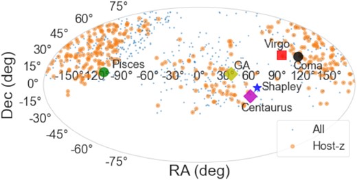
Sky distribution of the entire DR1 sample (DR1) with the subsample having host galaxy spec-z highlighted in orange. Known local overdensities, e.g. Coma (black circle), Virgo (red square), Great Attractor (yellow diamond), Shapley concentration (blue star), Pisces-Perseus cluster (green circle), Centaurus (magenta square), are highlighted for comparison.
Our sample uniquely features very early discoveries, with a median first detection epoch of −13.5 d, and densely sampled light curves. Recent studies in the literature (e.g. Hayden et al. 2019) propose improved standardization models using SN Ia data on the rise. They split the canonical light-curve shape parameter in SALT2 into |$x_1^{\rm r}$| and |$x_1^{\rm f}$| for the rising and falling part of the light curve and find that the two light-curve width model decreases the luminosity scatter. Our sample presented here is ideal for testing such novel standardization procedures that will be explored in follow-up studies on improving light-curve fitting algorithms.
We presented the SALT2 x1 and c parameter distributions in Fig. 6. We compared the distribution to the sample from the literature using a KS-test and found a low p-value for the x1 distributions, suggesting that they are not drawn from the same parent population. For the c-distribution, we find that the p-value is high indicating that, for the −0.3 < c < 0.3, the distributions are drawn from the same parent population. However, we find a larger fraction of c > 0.3 SNe Ia compared to the literature samples. We also present the stellar masses of the SN Ia host galaxies. We find a slightly larger fraction of low Mstellar host galaxies compared to the literature sample. We note that our requirement of having a spectroscopic redshift of the host can introduce selection effects in our host-z sample and will present a detail study of the entire DR1 host galaxy properties in a companion paper. For our sample, we compute the Hubble residuals and find an rms dispersion of 0.17 mag, comparable to the current state of the art in the literature. We emphasize that with ongoing improvements in the data processing this is expected to an upper limit on the scatter. We also simultaneously fit for σint using only the statistical errors from the light-curve fit and peculiar velocity errors and find a value of 0.15 mag.
ZTF completed phase I of observations in 2020 October, discovering and spectroscopically classifying > 3000 SNe Ia. In Fig. 9, we present the number of SNe discovered as a function of the time at which they peak (relative to the beginning of ZTF-I). We present these values for the entire ZTF-I using the photometry from the alerts computed by IPAC (see Masci et al. 2019, for details). We restrict the sample with quality cuts to the light-curve sampling as presented above and only show the SNe with an uncertainty on the inferred time of maximum of < 1 d. The full DR1 sample of 761 SNe Ia is already large enough we can start to test for anisotropies of the luminosity distance–redshift relation (e.g. Macpherson & Heinesen 2021). The complete ZTF-I sample after the quality cuts on the number of light-curve points and σ(t0) has >2400 SNe Ia. After applying the selection cuts for the gold sample based on SALT2 parameters, there are >1800 SNe Ia. We emphasize that these sample sizes are derived based on alert photometry that has very restrictive criteria and hence, with the photometry pipeline described in this work, we expect these numbers to improve further. With these large sample statistics, the already obtained ZTF-I data are competitve to measure local LSS properties, e.g. the growth rate, parametrized as fD (see Graziani et al. 2020, for more details). Analysing subsamples, based on host galaxy properties, from the complete ZTF-I data set based on host galaxy properties will be critical to study the origin of environmental systematics in SN Ia cosmology (Jones et al. 2018; Rigault et al. 2020).
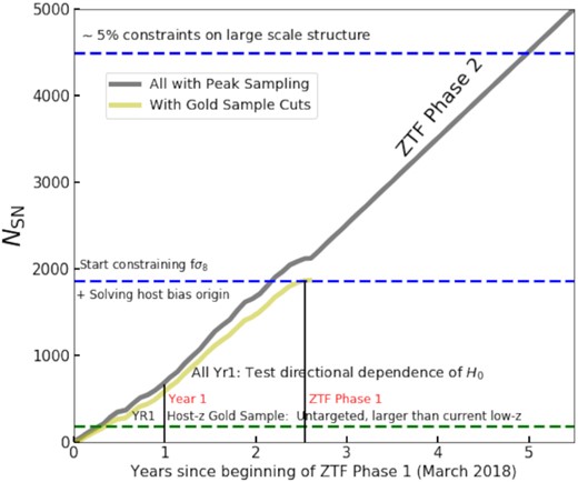
The number of SNe Ia with sufficient data for measuring distances discovered by ZTF-I and expected to be discovered by the ongoing ZTF-II as a function of time since the beginning of ZTF-I. The vertical lines mark the DR1 sample (present here) and the total ZTF-I sample.
We have ongoing efforts to improve the data reduction pipeline, obtain host galaxy spectroscopic redshifts, quantify systematic uncertainties, and, finally, constrain cosmological parameters. We expect the inferred intrinsic and rms dispersion values to decrease with improvements in the data processing. The size of the host-z as well as the complete DR1 samples is already at a stage where, with the improvements mentioned above, we can improve constraints on dark energy, measure H0, and the local bulk flow velocity. With the entire ZTF-I sample already acquired, we have sufficient number of SNe to obtain constraints on the growth of structure. This makes the ZTF data set exciting for answering various questions in cosmology.
SUPPORTING INFORMATION
Table 1. The SNe Ia in the complete Year 1 sample along with their coordinates, classification, first observation date, instrument from which the spectrum has been obtained, approximate resolution of the instrument, and date of first spectroscopic observation.
Table 2. SN names, heliocentric frame redshift, and coordinates (in degrees) for the SNe Ia in our sample. The table has been truncated for formatting reasons.
Table 3. Output SALT2 fit parameters for SNe in our sample along with the CMB frame redshift (zCMB; see the text for the CMB frame conversion).
Please note: Oxford University Press is not responsible for the content or functionality of any supporting materials supplied by the authors. Any queries (other than missing material) should be directed to the corresponding author for the article.
ACKNOWLEDGEMENTS
SD is supported by the Isaac Newton Trust and the Kavli Foundation through the Newton-Kavli fellowship and acknowledges a research fellowship at Lucy Cavendish College. AG acknowledges support from the Swedish Research Council under Dnr VR 2016-03274 and 2020-03444. MS, MR, and Y-LK have received funding from the European Research Council (ERC) under the European Union's Horizon 2020 research and innovation program (grant agreement No. 759194 – USNAC).
This paper is based on observations obtained with the Samuel Oschin Telescope 48-inch and the 60-inch Telescope at the Palomar Observatory as part of the Zwicky Transient Facility project. ZTF is supported by the National Science Foundation under Grant No. AST-1440341 and a collaboration including Caltech, IPAC, the Weizmann Institute for Science, the Oskar Klein Center at Stockholm University, the University of Maryland, the University of Washington, Deutsches Elektronen-Synchrotron and Humboldt University, Los Alamos National Laboratories, the TANGO Consortium of Taiwan, the University of Wisconsin at Milwaukee, and Lawrence Berkeley National Laboratories. Operations are conducted by COO, IPAC, and UW.
SED Machine is based upon work supported by the National Science Foundation under Grant No. 1106171. The ZTF forced-photometry service was funded under the Heising-Simons Foundation grant. This work was supported by the GROWTH project funded by the National Science Foundation under Grant No. 1545949.
Software: numpy (van der Walt, Colbert & Varoquaux 2011), astropy (Astropy Collaboration et al. 2013, 2018), sncosmo (Barbary et al. 2016), photutils (Bradley et al. 2019), ztfquery (Rigault 2018), swarp (Bertin 2010), hotpants (Becker 2015), zuds, fringez (Medford et al. 2021), matplotlib (Hunter 2007), IPAC forced Photometry Service, spextractor (Papadogiannakis 2019).
DATA AVAILABILITY
The data used in this study are made available on github at https://github.com/ZwickyTransientFacility/ztfcosmodr.
Footnotes
REFERENCES
APPENDIX A: PHOTOMETRY PIPELINE DESCRIPTION
In this section, we present a detailed description of the photometric pipeline parameters. As described in Section 2.5, the pipeline can be divided into three broad components, namely reference building, image subtraction, and forced photometry. Here, we describe each individual process.
A1 Reference building
Since the SNe Ia in our sample were discovered in 2018, in a fraction of the cases, the references for each field and read-out channel were created during the lifetime of the SN, which manifests itself as non-zero flux significantly before and after the inferred time of maximum. For example, some SNe Ia show negative flux in their forced photometry light curves before −30 d from the SALT2 t0 time, since there is SN flux in the reference image. In our custom pipeline, we use images at least 30 d before peak to make deep references. For SNe with insufficient data (<30 frames) in the phase range before −30 d, we also use data from >400 d after peak. For each reference image, we have quality control selection cuts such that only images within the seeing range 1.7 and 3 arcsec and a nightly magnitude limit fainter than 19.2 mag are used in the final reference creation.
We use swarp on the processed images from IPAC to make the reference. For each input image, we create a test weight map with the mask image from IPAC as an input (Masci et al. 2019). The weight map is passed as an to SE xtractor to create an rms map for each input image that goes into making the final reference image. Each associated weight map, derived from the SE xtractor output rms map, is input along with the image to make the reference coadd. Before coadding, the input images are all scaled to a common zero-point magnitude of 25. The associated reference mask is produced by using the logical AND function with swarp to combine the individual epoch masks. This is because logical OR coaddition is extremely restrictive at masking the reference image.
A2 Image subtraction
The individual science frame, and the associated mask and rms file, along with the reference coadd and its associated mask and rms file are input to the image subtraction routine. As described in Section 2.5, we use hotpants (Becker 2015) for the difference imaging part of the pipeline. For both the science image and the reference, we fix the lower valid data count as the computed background minus 10 times the standard deviation. For the differencing, we use a convolution kernel with a half-width that is 2.5 times the seeing and a half-width of the substamp to extract around each centroid as six times the seeing. We set the normalization to the science image and convolve to the reference image.
A3 Forced photometry
We use the astropy package photutils (Bradley et al. 2019) to perform aperture photometry. We define the aperture using the SkyCircularAperture function with a 6-pixel diameter aperture. The location is defined as the median coordinate in each filter, derived from the alert packets (see Fremling et al. 2020, for details). We apply a correction for a six pixel aperture to the final zero-point for the observed fluxes, as provided in the IPAC data products.
