


ABSTRACT
Using action-based distribution function for the dynamical model of the Milky Way (MW) we have estimated its total mass and its density profile. Constraints are coming from the globular cluster proper motions from Gaia EDR3, from the rotation curve based on Gaia DR2 data, and from the vertical force data. We use Bayesian Markov chain Monte Carlo method to explore the parameters, for which the globular cluster distribution function and the Galactic potential are fully constrained. Numerical simulations are used to study the uncertainties on the potential constraint if considering a possible massive Large Magellanic Cloud (LMC). We found that a massive LMC (1.5 × 10¹¹ M⊙) will affect the MW mass measurement at large radius, which includes both the MW and the LMC. We also use the FIRE2 Latte cosmological hydrodynamic simulations to make mock data set from an MW-like galaxy that includes many unrelaxed substructures. We test the effect of these unrelaxed substructures on the final results, and found that the measured rotation curve fluctuated around input value within 5 per cent. By keeping a large freedom in choosing a priori mass profile for both baryonic and dark matter leads a total mass of the MW that ranges from |$5.36_{-0.68}^{+0.81}\times 10^{11}$| M⊙ to |$7.84_{-1.97}^{+3.08} \times 10^{11}$| M⊙. This includes the contribution of a putative massive LMC and significantly narrows the MW total mass range published earlier. Such total mass leads to dark matter density at solar position of |$0.34_{-0.02}^{+0.02}$| GeV cm−3.
1 INTRODUCTION
The Galactic dark matter (DM) mass density profile and total mass are of the most importance in modern astrophysics and cosmology. The Milky Way (MW) provides a unique opportunity for testing cosmology at small scales and the galaxy formation process. The mass density profile and the total mass of the MW governs its number of sub-haloes of MW mass galaxies, which is intimately related to low-mass scale discrepancies to standard cold dark matter model (ΛCDM). For example, the missing satellite and the too-big-to-fail problems (Moore et al. 1999; Boylan-Kolchin, Bullock & Kaplinghat 2011; Wang et al. 2012; Cautun et al. 2014) are all closely related to the total mass of MW. Therefore, the accurate measurement of the total mass of MW is also important for understanding dwarf dynamics and their accretion history, and also tests cosmological predictions. Gaia (DR2 and even more EDR3) data become sufficiently precise to constraint the orbital properties of MW dwarfs. It can be used to further test whether the MW and its cortege of dwarfs are similar to ΛCDM halo and sub-haloes (Riley et al. 2019; Hammer et al. 2020; Li et al. 2021), which again depends on the MW total mass.
The elusive DM emits no light and can be only detected using indirect methods. Since DM affects dynamics, the kinematics of various luminous tracers have been investigated to derive its mass and density profile. In the inner region, the disc rotation curve (RC) is usually measured with tracers having circular motions, for instance, classic Cepheids (Mróz et al. 2019), open clusters, H ii region (Sofue 2012). In the halo region, the DM mass density profile is usually derived from kinematic analysis from halo tracers, for examples, dwarfs assumed to be long-lived satellites (Callingham et al. 2019), globular clusters (Eadie & Jurić 2019; Vasiliev 2019b; Watkins et al. 2019), stellar streams (Gibbons, Belokurov & Evans 2014; Bowden, Belokurov & Evans 2015; Küpper et al. 2015; Malhan & Ibata 2019), and halo stars (Kafle et al. 2012, 2014). A comprehensive review on the methods of total Galactic mass measurement can be found in Wang et al. (2020). Even though the total mass of MW has been measured for a few decades, its actual value is still uncertain by a large factor (see fig. 1 of Wang et al. 2020).
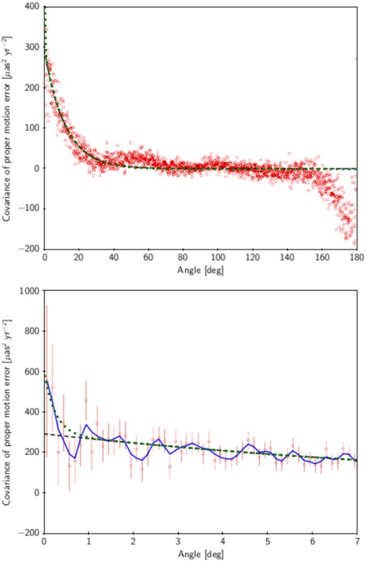
The covariance of proper motion of data in Gaia EDR3. This figure is from fig. 15 of Lindegren et al. (2020), except adding the new fitting curve (the dotted-green line) from equation (1). The open red circles are individual estimates and the black-dash line is an exponential fitting. The top panel shows the large separation, while the bottom panel shows results for small separation angle. The individual estimates and the fitted black-dash line are from Lindegren et al. (2020). The blue-solid line indicates the smoothed covariance values from Lindegren et al. (2020). The green dashed line is our modified fitting to the exponential fitted result as shown by equation (1).
The Gaia satellite has revolutionized the Galactic mass determination by providing accurate proper motion for a far much larger number of stars than ever done before. By combining the large sky spectroscopic survey in the ground such as SDSS (York et al. 2000) and LAMOST (Cui et al. 2012; Zhao et al. 2012), accurate 6D phase-space coordinates can provide strong constraint on the Galactic DM profile and total mass. It is expected in the following years that the Gaia will continue to improve precision and accuracy of the astrometry and photometry for more and more stars (Gaia Collaboration 2021).
Understanding how the MW is structured and its assembly history is now a central task in using those unprecedented data. Dynamical modelling is one of most important tools to understand how the MW is structured. Dynamical modelling with action-based distribution function DF (|$f(\boldsymbol{J})$|) has provided a major progress in this field. In an axisymmetric system, the action integrals |$\boldsymbol{J}_r$|, |$\boldsymbol{J}_z$|, |$\boldsymbol{J}_\phi$| are the integral of motions, quantifying the amplitude of oscillations in the radius and in the vertical directions, and angular momentum around the symmetric axis, respectively (Vasiliev 2019a; Binney 2020). These actions are adiabatically invariants and conserved under slowly evolution of the potential, and in absence of energy exchanges. Consequently, |$f(\boldsymbol{J})$| is invariant too. A system is fully determined as long as the DFs of each component are specified, and from these DFs any measurement can be predicted for the model (Binney 2020).
Recent progresses with large spectroscopic surveys and Gaia data reveal that the stellar halo is made of unrelaxed substructures and furthermore there might be a large-scale velocity gradient induced by the passage of the Large Magellanic Cloud (LMC), if the latter is very massive. These two effects may affect the assumption of equilibrium and relaxed system in any dynamical modelling, which should be addressed when interpreting modelling results.
In this work, we use new released data of Gaia EDR3 to derive the proper motion of Galactic globular clusters. The improvement by about a factor of 2 in proper motion and the similar reduction of the systematic error (Gaia Collaboration 2021) make the measurement on the MW DM density profile improvement much better than ever. Combining the new data with the accurate disc RC from Gaia DR2 (Eilers et al. 2019), we can model the Galactic globular clusters (GCs) with the action-based distribution function, and then constrain Galactic DM profile. By using N-body simulation one can test the bias introduced by a possible massive LMC. By using realistic cosmological hydrodynamic simulations from the FIRE2 suite, we can test the effects of unrelaxed substructures.
The paper is organized as follows: Section 2 presents the measurement of GC proper motions and their uncertainties with Gaia EDR3. Section 3 describes the additional observation data used to constrain the RC measurement. Section 4 presents the detail on the dynamical modelling with action-based DF method, and the results are shown in Section 5. In Section 6, we use numerical simulations to investigate the possible effect of a massive LMC passing by to the MW mass measurement, as well as the effects due to unrelaxed substructures. Lastly, we conclude our results in Section 7.
2 THE PROPER MOTION OF MW GCS
In this section, we describe the method used to derive the mean proper motion and its associated uncertainties considering the systematic errors in the Gaia EDR3.
2.1 Determining the mean proper motions of GCs with Gaia EDR3
We follow the procedure of Vasiliev (2019b) to derive the mean proper motion (PM) and its associated uncertainties for each cluster. We have used the publicly released code by Vasiliev (2019b). Here, we briefly describe the method (more details in Vasiliev 2019b, c).
The stars around each GC are clumped in PM space, which include member stars and field stars. For each cluster, a probabilistic Gaussian mixture model is applied to the PM distribution for stars and determines their membership probability. A spherical Plummer profile is assumed for the prior functional form of membership probability, for which the scale radius of Plummer profile is allowed to be adjusted during the fitting. An isotropic Gaussian function is assumed for the intrinsic PM dispersion for the cluster members. By adopting this spatially dependent prior for the membership probability, the intrinsic (error-deconvolved) parameters of the distributions of both member and non-member stars are derived. Since there are non-negligible spatially correlated systematic errors in the PM of Gaia data, this systematic error can be addressed by adopting the PM correlation function as below.
Fig. 1 details how this covariance function fit to the angular covariance of proper motion from high precision quasar from Lindegren et al. (2020), as well as comparing to the fitting with single exponential function from Lindegren et al. (2020). The new fitting function of equation (1) fit the covariance well for both large-scale and central regions.
2.2 Robustness of GC proper motions
To have a clean sample with reliable astrometric measurements of the PM, we follow the recommendations of Fabricius et al. (2021): (1) renormalized unit weight error (RUWE) <1.2, (2) asymmetric_excess_noise <1.0, (3) ipd_gof_harmonic_amplitude <0.1, (4) ipd_frac_multi_peak <2, (5) the corrected excess factor (Ccorr) within 3σ following Riello et al. (2021).
Fig. 2 compares our measured proper motion, its associated uncertainties and correlation coefficient, and the internal dispersion with that from Gaia DR2 from Vasiliev (2019b).
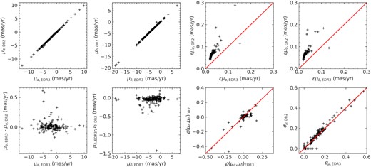
Comparing proper motion measurement between Gaia EDR3 of this work and DR2 from Vasiliev (2019b). The panels on the top row show the one-by-one comparison of proper motion in two directions μα, μδ, and their errors. The left two panels in the bottom row show the difference of proper motion in two directions as function of proper motions. The third panel of bottom row shows the comparison of correlation coefficience of proper motion. The fourth panel shows the internal dispersion of proper motion (for details please refer to Vasiliev 2019b).
The first two panels in the top-left compare the proper motion of |$\mu _\alpha ^{*}$| and μδ from DR2 and EDR3 and they correlate well. In the first two panels in the bottom-left, we show the absolute differences of proper motion as a function of |$\mu _\alpha ^{*}$| and μδ, respectively. The absolute difference in proper motion is reasonably small, in most cases lower than 0.1 mas yr−1.
In the two panels in the top-right, we compare the measured uncertainties of proper motions. The errors in EDR3 are systematic smaller than that from DR2 by about a factor of 2, which is fully consistent with Gaia Collaboration (2021).
The third panel in the bottom row compares the correlated coefficients. The coefficients are well correlated, which shows that the correlation coefficients do not change too much even though the error of PM has decreased a factor of 2. The last panel of the bottom row compares the internal dispersion. The internal dispersion is correlated between DR2 and EDR3, which probability indicate that this method has well resolved the intrinsic dispersion for each cluster.
After finishing this work, we notice Vasiliev & Baumgardt (2021) have measured the PM for GCs with Gaia EDR3 with an updated method comparing to Vasiliev (2019b) with a more strict selection criteria to clean the data. We have compared their results with ours (Fig. 3) and find that it would not introduce significant differences in the final results as discussed in Appendix B.

3 DATA USED TO CONSTRAIN MW MASS MODELLING
Besides GCs, here we describe other kinematic data set used to constrain the dynamic models for MW.
3.1 Circular velocity from Gaia DR2
The RC of the disc has been estimated by various tracers. By using the accurate proper motion from Gaia DR2 combining with precise spectrophotometric parallax from APOGEE DR16, Eilers et al. (2019) have derived disc RC for Galactocentric distance of 5 ≤ R ≤ 25 kpc with high precision for ∼23 000 red giants. They have applied Jeans equation after assuming an axisymmetric gravitational potential to obtain this measurement. This result has been found consistent with measurement from Classic Cepheids (Mróz et al. 2019; Ablimit et al. 2020).
The precise distance and proper motion have led to the most precise RC derived to date (Eilers et al. 2019), i.e. with much smaller error bars than that of former studies. Eilers et al. (2019) have also analysed systematic errors from various assumption. As mentioned by Jiao et al. (2021) that summing up all errors will dilute the significance of RC. Therefore, following Jiao et al. (2021) we added the systematic error of the cross-term in the radial and vertical velocity to the total error budgets. We noticed that this precise RC data have already been used to estimate MW mass (Karukes et al. 2020).
This data will provide constraints on the disc RC for our modelling.
3.2 Vertical force at z = 1.1 kpc
Piffl et al. (2014) showed that the vertical force brings an important constraint to the DM shape, which has been widely used in the literature for estimating the MW potential (Bovy 2015; Bovy et al. 2016; McMillan 2017; Hattori, Valluri & Vasiliev 2021). By using Jeans equation, Kuijken & Gilmore (1991) measured vertical force, Kz,1.1kpc at z = 1.1 kpc away from the disc. Bovy & Rix (2013) using SDSS/SEGUE data measured the vertical force Kz,1.1kpc(R) as function of radius, which is used in our analysis. As mentioned by Hattori et al. (2021), the RC of Eilers et al. (2019) provides the radial force constraint on the model, while the Kz,1.1kpc(R) gives an independent constraint on the vertical direction.
4 MODELLING
In the following sections, we describe how the modelling for the GC DF has been set-up. We note the six GCs associated with Sagittarius galaxy (NGC 6715, Terzan 7, Terzan 8, Arp 2, Pal 12, and Whiting 1), which we have excluded in the analysis following Vasiliev (2019b) and Myeong et al. (2019) and since they are clustering in the phase-space diagram. There could be other GCs associated with different accretion events (Massari, Koppelman & Helmi 2019) and they are included in current analysis. However, in Section 6.3 we verify that unrelaxed substructures do not have significant effect on the final results, on the basis of an analysis made using the FIRE2 suite of simulations.
4.1 Models for the galactic gravitational potential
In this work, we use axisymmetric Galactic potential Φ(R, z), which consist of baryon mass components and DM. In order to determine the DM mass profile, we first specify the adopted baryon mass model that follows McMillan (2017), and which include multicomponents (a bulge, a thin and a thick stellar disc, an H i disc and a molecular gas disc).
Jiao et al. (2021) investigated different baryonic mass profiles to test the MW DM distribution. Here, we prefer to adopt a baryonic mass profile that also includes the gas contribution. Given the fact that baryons are not the dominant component, this should not alter our main conclusions.
4.1.1 The bulge
There is a bar in the central region of the MW, which introduces non-axisymmetric potential. In this work, we use the software agama (Vasiliev 2019a) to deal with actions with Stäckel fudge method, which can only handle oblate axisymmetric potentials. Therefore, the central region is not expected to be well modelled. Following the literature (Vasiliev 2019b; Cautun et al. 2020; Hattori et al. 2021), the parameters r0, α, rcut, and a parameters are fixed during the modelling procedure, and their values are listed in Table 1. Following Cautun et al. (2020), the scale density of ρ0,bulge has a Gaussian prior value of 100 ± 10 M⊙ pc−3.
Parameters of baryon gravitational potential are fixed in the dynamical model.
| HI disc | H2 disc | Units | |
|---|---|---|---|
| Σ0 | 53.1 | 2179.5 | |$\mathrm{ M}_\odot \, \rm{pc}^{-2}$| |
| |$R_{\rm \mathrm{ d}}$| | 7.00 | 1.5 | kpc |
| |$z_ {\rm \mathrm{ d}}$| | 0.85 | 0.045 | kpc |
| |$R_{\rm {\mathrm{ hole}}}$| | 4 | 12 | kpc |
| Stellar thin disc | Stellar thick disc | Units | |
| |$z_{\rm \mathrm{ d}}$| | 0.3 | 0.9 | kpc |
| Stellar bulge | Units | ||
| r0 | 0.075 | kpc | |
| |$r_{\rm {\mathrm{ cut}}}$| | 2.1 | kpc | |
| α | 1.8 | ||
| q | 0.5 |
4.1.2 The thin and thick stellar disc
Here, zd denote the scale height for the disc. Following McMillan (2017), we set zd to be 0.3 and 0.9 kpc for thin and thick disc, and keep fixed during our modelling process. Σ0 and Rd indicate the centre surface density and scale length for the discs. These two parameters for each disc component are not fixed, but fitted with Gaussian prior values. These prior values are from McMillan (2017), except for the thick disc scale length (Rd), for which we adopt a value from 3.5 kpc from Bland-Hawthorn & Gerhard (2016) and Cautun et al. (2020). A 30 per cent uncertainty is adopted for the Σ0 and Rd during the fitting.
4.1.3 The molecular and atomic gas discs
These models are kept fixed during the procedure. In the model, the mass of HI is 1.1 × 10¹⁰ M⊙, and the molecular gas mass is around 10 per cent of the HI.
4.1.4 The dark matter halo
We chose two well-known and used mass profiles to get flexible the slope of DM density at outskirts, one follows Zhao (1996, hereafter called ‘Zhao’) and the other Einasto (1965, hereafter called ‘Einasto’).
In the case of α = 1, β = 3, and γ = 1, the profile corresponds to the NFW profile, which is widely used in the literature for representing DM haloes. Comparing to the NFW profile, the Zhao’s profile has more flexibility.
There are three parameters in the Einasto profile, which has been argued to provide the best description of the DM profile (Gao et al. 2008; Bullock & Boylan-Kolchin 2017).
The determination of Galactic DM shape is important to constraint cosmological models. The shape of DM halo is triaxial (Jing & Suto 2002) in DM-only simulation, and this can be affected by the inclusion of baryonic component. Chua et al. (2019) using Illustris suite of simulation found that the DM halo has an oblate-axisymmetric shape with a minor to major ratio of 0.75 ± 0.15. The MW dark halo shape has been measured with various methods. Wegg, Gerhard & Bieth (2019) used RR Lyrae stars and they found the flattening of DM halo q = 1.00 ± 0.09, based on the axisymmetric Jeans equation. The GD-1 stream kinematics has been used to measure the Galactic DM shape, and Malhan & Ibata (2019) found |$q=0.82\pm ^{+0.25}_{-0.13}$|, while Bovy et al. (2016) gave |$q=1.3\pm ^{+0.5}_{-0.3}$|. Vasiliev, Belokurov & Erkal (2021) modelled the Sagittarius stream considering the effect of a massive LMC on the MW using an oblate DM halo, which becomes triaxial beyond 50 kpc. With axisymmetric Jeans equations, Loebman et al. (2014) considered SDSS halo stars and estimated the MW DM density flattening to be q = 0.4 ± 0.1. Therefore, the large range of q from different observations leads us to use a large range of flattening parameters for the modelling.
During the modelling, the halo shape is not spherical, and we have let the halo shape parameter q free varying from 0.1 to 1, which corresponds to an oblate shape (q ≤ 1). In current studies, we are limited to oblate haloes, which is a restriction due to the agama software (Vasiliev 2019a). The lower limit is set to avoid calculation divergence.
All of the parameters for the two DM halo profiles are free in our modelling. In Table 2, all free parameters of the modelling are listed. Even though halo parameters are limited to ranges listed in Table 2, we have checked the Markov chain Monte Carlo (MCMC) chains for each parameter to be sure that parameters have been explored in sufficiently large ranges, to ensure the absence of non-investigated solutions.
The model parameters used in our modelling. The best derived values are shown with median and 68 percentile of the posterior distribution. Gaussian prior functions have been used for baryon model parameters, while flat prior has been adopted for all the other parameters. The ranges of parameters in the prior have been chosen which are large enough without imposing constraints on the parameters sampling with MCMC when checking the MCMC chains. The low limit of out slope (β) for DM profile in Zhao is set to 2, and 0 for Einasto profile.
| Parameters | Symbol | Units | Prior | Best-fitting values | |
|---|---|---|---|---|---|
| Einasto halo | Zhao’s halo | ||||
| Gravitational potential | |||||
| Baryon gravitational potential | |||||
| bulge density | |$\rho _{0,\rm bulge}$| | M⊙ pc−3 | 100 ± 10 | |$94.64_{-9.76}^{+9.35}$| | |$95.20_{-11.79}^{+9.90}$| |
| thin disc density | |$\Sigma _{0,\rm thin}$| | M⊙ pc−2 | 900 ± 270 | |$1057.50_{-89.42}^{+87.71}$| | |$1003.12_{-130.70}^{+134.77}$| |
| thick disc density | |$\Sigma _{0,\rm thick}$| | M⊙ pc−2 | 183 ± 55 | |$167.76_{-54.09}^{+57.40}$| | |$167.93_{-54.06}^{+60.09}$| |
| thin disc scale length | Rthin | |$\, \mathrm{kpc}$| | 2.5 ± 0.5 | |$2.39_{-0.11}^{+0.11}$| | |$2.42_{-0.13}^{+0.15}$| |
| thick disc scale length | Rthick | |$\, \mathrm{kpc}$| | 3.5 ± 0.7 | |$3.20_{-0.54}^{+0.52}$| | |$3.17_{-0.54}^{+0.56}$| |
| DM density profile | |||||
| DM density | ρ0 | |$~\mathrm{M}_\odot \, \mathrm{kpc}^{-3}$| | 0 < log10ρ0 < 15 | |$9.29_{-0.21}^{+0.20}$| | |$7.19_{-0.51}^{+0.38}$| |
| DM scale length | rh | |$\, \mathrm{kpc}$| | −2 < log10rh < 4.5 | |$-1.40_{-0.26}^{+0.26}$| | |$1.07_{-0.21}^{+0.24}$| |
| Inner slope | γ | – | 0 < γ < 3 | – | |$0.95_{-0.32}^{+0.31}$| |
| steepness | α | – | 0 < α < 20 | – | |$1.19_{-0.25}^{+0.33}$| |
| Outer slope | β | – | 2Zhao, 0Eina < β < 20 | |$0.32_{-0.02}^{+0.02}$| | |$2.95_{-0.41}^{+0.51}$| |
| axial ratio (z/R) | q | – | 0.1 < q < 1 | |$0.97_{-0.06}^{+0.03}$| | |$0.95_{-0.07}^{+0.04}$| |
| Distribution function of GCs | |||||
| slopeOut | B | – | 3.2 < B < 10 | |$5.03_{-0.64}^{+1.88}$| | |$4.61_{-0.35}^{+0.71}$| |
| slopeIn | Γ | – | 0.1 < Γ < 2.8 | |$1.23_{-0.28}^{+0.26}$| | |$1.14_{-0.34}^{+0.32}$| |
| steepness | η | – | 0.5 < η < 2.0 | |$1.08_{-0.37}^{+0.52}$| | |$1.29_{-0.39}^{+0.39}$| |
| coefJrOut | gr | – | 0.1 < gr < 2.8 | |$0.65_{-0.13}^{+0.12}$| | |$0.71_{-0.12}^{+0.14}$| |
| coefJzOut | gz | – | 0.1 < gz < 2.8 | |$1.32_{-0.13}^{+0.11}$| | |$1.32_{-0.12}^{+0.13}$| |
| coefJrIn | hr | – | 0.1 < hr < 2.8 | |$1.86_{-0.29}^{+0.31}$| | |$1.81_{-0.37}^{+0.32}$| |
| coefJzIn | hz | – | 0.1 < hr < 2.8 | |$1.01_{-0.30}^{+0.29}$| | |$1.01_{-0.34}^{+0.32}$| |
| J0 | J0 | – | |$-2\lt \log _{J_0}\lt 7$| | |$3.08_{-0.22}^{+0.45}$| | |$2.94_{-0.18}^{+0.21}$| |
| rotFrac | κ | – | −1 < κ < 1 | |$-0.94_{-0.04}^{+0.08}$| | |$-0.93_{-0.05}^{+0.10}$| |
| Derived quantities | |||||
| bulge mass | |$M_{\star ,\rm bulge}$| | 1010 M⊙ | – | |$0.85_{-0.08}^{+0.09}$| | |$0.86_{-0.11}^{+0.09}$| |
| thin disc mass | |$M_{\star ,\rm thin}$| | 1010 M⊙ | – | |$3.79_{-0.30}^{+0.28}$| | |$3.69_{-0.37}^{+0.34}$| |
| thick disc mass | |$M_{\star ,\rm thick}$| | 1010 M⊙ | – | |$1.03_{-0.39}^{+0.47}$| | |$1.05_{-0.45}^{+0.53}$| |
| M200 | |$M_{200; \ \rm MW}$| | 1011 M⊙ | – | |$5.73_{-0.58}^{+0.76}$| | |$7.84_{-1.97}^{+3.08}$| |
| R200 | |$R_{200; \ \rm MW}$| | |$\, \mathrm{kpc}$| | – | |$170.7_{-5.9}^{+7.2 }$| | |$189.5_{-17.4}^{+22.1}$| |
| Vescaped at sun | vesc, ⊙ | |$\, \mathrm{km}\, \mathrm{s}^{-1}$| | – | |$495.5_{-9.7}^{+11.2}$| | |$528.3_{-31.4}^{+55.3}$| |
| DM density at sun | ρDM, ⊙ | GeV cm−3 | – | |$0.34_{-0.01}^{+0.02}$| | |$0.34_{-0.02}^{+0.02}$| |
4.2 Distribution function
By assuming that the GC system is in dynamical equilibrium, the distribution function (DF) of GCs can be expressed in phase-space by a function of |$f(\boldsymbol{J})$| with three actions, |$\boldsymbol{J}=(J_r, J_z, J_\phi)$|, where Jr and Jz is the radial and vertical actions, and Jϕ is the azimuthal action and equal to angular momentum in the z component.
The dimensionless parameters (gr, gz, gϕ) and (hr, hz, hϕ) control the density shape and the velocity ellipsoid in the outer region and inner region (Posti et al. 2015; Das & Binney 2016; Das, Williams & Binney 2016; Vasiliev 2019a), respectively. gi and hi have been constrained by Σihi = Σigi = 3 (Vasiliev 2019a). In this way, the degeneracy between gi and hi and |$\boldsymbol{J}_0$| will be broken (Das & Binney 2016; Das et al. 2016). The power-law indices B and Γ are related to the outer and inner slope, while η determines the steepness of this two regime transition. The parameter κ controls the net rotation of the system, with κ = 0 being the non-rotation case, and κ = ± 1 indicate the maximal rotation case. In the publicly released version of agama (Vasiliev 2019a), |$\boldsymbol{J}_\phi$| is normalized by a fixed constant, which leads to a non-rotating core. Following Vasiliev (2019b), we have modified the publicly released software agama, in the way that the |$\boldsymbol{J}_\phi$| is normalized by the value summarizing three actions and the rotation will be roughly constant at all energies. The total mass is the normalization parameter.
4.3 Error models for observables
Observations of the GC system are not error free. In the following, we consider Gaussian models for the error to associate the true quantities with observables and its errors. The six observables for GCs are |$\bar{u}$||$= (l, b, s, v_{\mathrm{los}}, \mu _\alpha ^{*}, \mu _\delta)$|, where (l, b) denote the Galactic longitude and latitude that are measured with high precision so their errors are neglected in the following analysis. The heliocentric distance is s and its error is not neglected. Following Vasiliev (2019b), we adopted a 0.046 per cent uncertainty (correspond to 0.1 in distance modulus). vlos is the line-of-sight velocity, and its value is taken from the table C1 of Vasiliev (2019b). The proper motion is derived from the above study, and the correlated uncertainties in |${\bf \mu }=(\mu _\alpha ^{*}, \mu _\delta)$| as well as the covariance matrix (Σμ) are taken into account.
4.4 The Bayesian inference
4.4.1 Likelihood for the GC distribution function
4.4.2 Likelihood from the disc circular data
The precise RCs in the disc region have been derived by Eilers et al. (2019), which can provide constraints on the total potential and can help to break the degeneracy between baryonic and DM contributions to the potential. This motivates us to include RC data into our modelling with the Bayesian theorem.
4.4.3 Likelihood for the vertical force Kz,1.1 kpc
4.4.4 Total likelihood
4.4.5 The priors
In the Bayesian inference, we can put priors to constrain the amplitude of parameters. Our priors are listed in Table 2. The prior in the baryon gravitational potential is mostly taken from McMillan (2017), Deason et al. (2021), and Bland-Hawthorn & Gerhard (2016), and a Gaussian function is adopted for the prior function. For the parameters related to the DM profile and DF of GCs, the priors are set as uniform within the reasonable ranges listed in Table 2. In the cold dark matter (CDM), the DM halo follows a cuspy density profile with γ ∼ 1 (NFW); however, the observed RC of local spirals seems to be more consistent with core density profile with γ ∼ 0. The core density profile is also reasonable for dwarf spheroidal galaxies and Low Surface Brightness (LSB; see Di Matteo et al. 2008 for discussion). The situation becomes more complex if the DM profile is modified after the inclusion of baryons (Cautun et al. 2020), which results in the fact that neither NFW nor the generalized NFW succeeded to fit the MW RC data. However, Jiao et al. (2021) found that a nearly flat density core with Einasto profile is best for MW DM density profile, including baryons or not. Based on the above discussion, we decide to adopt non-informative flat priors for the DM profile parameters. For the parameters relevant to the DF of GCs, we chose uniform priors following the literature (Binney & Wong 2017; Posti & Helmi 2019; Vasiliev 2019b). We have visually checked the posterior distribution for the MCMC chains to be sure that the prior range is large enough and does not impose constraints on the parameters sampling.
4.5 Model parameter estimates
We use the Nelder–Mead method implemented in the python scipy package to maximize the above likelihood, and find the parameters with maximum likelihood. By using these parameters as initial input values, we use MCMC method to explore the parameter space, which is implemented in the emcee package (Foreman-Mackey et al. 2013). To be sure a converged result achieved with MCMC, we run ∼10 × Npars (where Npars is the total number of free parameters) walkers for the modelling of the GC system, and ∼5 × Npars for the mock simulation data in Section 6. The MCMC is ran for several thousand steps to be sure to achieve a converging result, and in the following analysis, the first half chain is discarded for the initial burn-in chain. We use the median value of the posterior distribution for the estimated results, and 68 percentile for the credible intervals. We point out that 68 percentile does not reflect a one σ error bar since the marginal posterior distribution is non-Gaussian.
5 RESULTS ON THE MW MASS
5.1 The posterior distribution of parameters
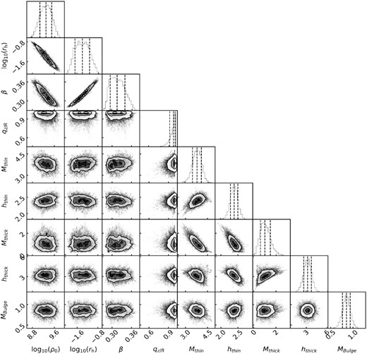
In this section, we examine the final results from analysing the posterior distribution. To have an overall view about the estimated parameters of our modelling, we show the posterior distribution of the inferred parameters with Zhao DM density profile (equation 6) in Figs 4 and 5. The posterior distribution of estimated parameters are separated into gravitational potential fields (Fig. 4) and distribution function of GCs (Fig. 5), respectively. The posterior distribution of parameters shows that they converge well. The final results are listed in Table 2 in the last columns, with both the DM density profiles for Einasto (equation 7) and Zhao (equation 6) models.
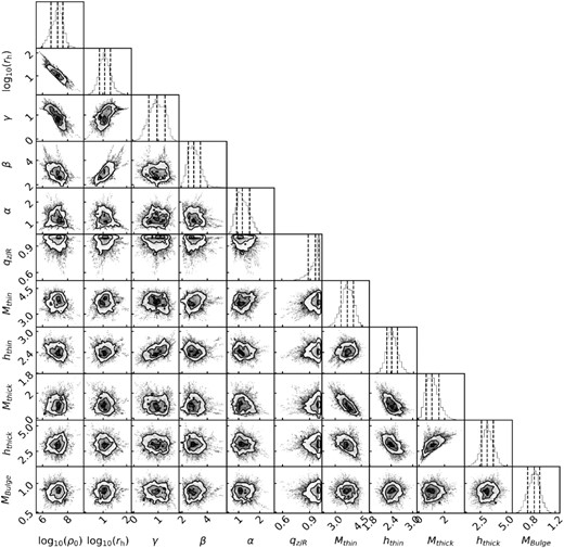
Posterior distribution of parameters for potential fields with model using the Zhao’s DM density profile (equation 6). The parameters log ρ0, log ascale, γ, β and α, are for parameters of DM mass distribution. The parameters Mthin, Mthick, Mbulge are total mass for the thin and thick disc, and bulge components, with units in 1010 M⊙. The parameters hthin, hthick indicate the scale length for thin and thick disc, respectively. Contour lines in each panel and the vertical lines in the marginal histograms show the 16 per cent, 50 per cent, 84 per cent percentiles.
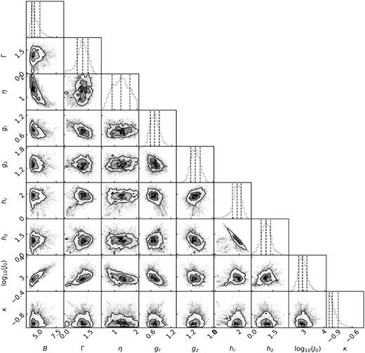
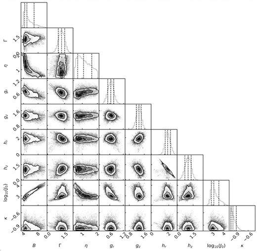
Posterior distribution of parameters of DF (equation 8) of GCs with model using the Zhao’s DM density profile (equation 6). The parameters B and Γ related to the outer and inner slopes of DF, while η determines the steepness of transition. The dimensionless parameters gr, gz, hr, hz control the density shape and the velocity ellipsoid in the outer and inner region. The inner and outer regions are separated with actions J0. κ that control the rotation. Contour lines in each panel and the vertical lines in the marginal histograms show the 16 per cent, 50 per cent, 84 per cent percentiles.
5.2 Fits of the observational data
Even though we have adopted the similar modelling method as in Vasiliev (2019b), there are two major differences with them. First, we have used Gaia EDR3 that improves the uncertainties by a factor of 2. Secondly, we have added two important tight constraints by imposing the model to fit both the MW RC and the vertical force data. It would be useful to check how the DF different to that of Vasiliev (2019b).
Following Vasiliev (2019b), we have derived from our posterior distribution the velocity structure variation and the axial ratio of GCs as a function of the radius as it is shown in Fig. 6. The velocity anisotropic parameter β varies with radius, being isotropic in the centre and radially dominated at the outskirts. The axial ratio q increases with radius, which is consistent with the disc component in the inner region (Binney & Wong 2017).
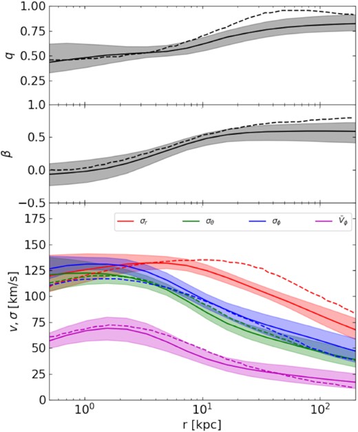
Physical quantities estimated from ensemble of models from MCMC runs in function of radius. The solid lines are the mean values estimated from MCMC models, while the shaded regions indicate the 68 per cent credible regions. Top panel: the axial ratio (q = z/R) of GCs spatial density profile varied as function of radius. Middle panel: the velocity anisotropic parameter |$\beta = 1-(\sigma ^2_{\theta }+\sigma ^2_{\phi })/(2\sigma ^2_r)$| in function of the radius. Bottom panel: the velocity dispersions in three directions and the mean azimuthal velocity as function of the radius. For comparison, the dotted lines in each panel show the results from Vasiliev (2019a).
Fig. 6 shows our modelling results of GCs and compares them to that of Vasiliev (2019a). The velocity dispersion, anisotropic parameter, and axial ratio of GCs are found to be very similar; however, the radial velocity dispersion shows large discrepancy at r > 10 kpc from one to the other study.
Fig. 7 compares the vertical force Kz = 1.1 kpc from the observed data (Bovy & Rix 2013) and that derived from our posterior distribution. The model reproduces well the observed vertical force.
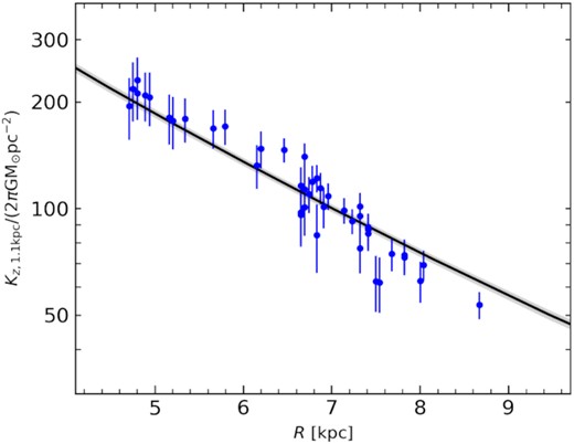
The vertical force at z = 1.1 kpc as function of radius. The blue solid circle and error bars are from the observation measurements by Bovy & Rix (2013), and the black line and shaded region indicate the estimated and 68 percentile of posterior distribution of our model.
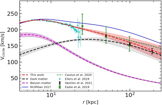
5.3 The Milky Way rotation curve
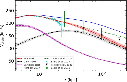
Fig. 8 shows the RCs derived from our new modelling with Zhao’s DM density profiles (equation 6, the red-line and shaded region). The derived RC is fitting well the disc RC of Eilers et al. (2019), for which velocities are much lower than that predicted by McMillan (2017). The RC from Zhao’s DM profile is consistent with the recent results of Vasiliev et al. (2021) and Eadie & Jurić (2019), as shown in Fig. 8. Cautun et al. (2020) have also fitted the disc RC of Eilers et al. (2019) considering the baryon contraction effect. They considered constraints from dwarf satellites based on Callingham et al. (2019), which results in a higher value of RC at outskirts than our value.
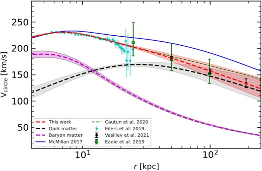
It compares RCs derived from posterior distribution of our models with literature. The Zhao’s DM model is used. The shaded region indicates the 68 percentile. The black dashed line indicates the contribution from DM, while the magenta dashed line shows the contribution from baryon matter.
5.4 Escaped velocity and DM density at solar position
Accurately deriving the DM mass density profile means that we can make predictions on the escaped velocity and the DM density at solar position, and compare them with different measurements in the literature. Fig. 9 shows the probability distribution function (PDF) of the escaped velocity at solar position. Our value is consistent with the most recent results on the escaped velocity measurement (Deason et al. 2019a; Necib & Lin 2021). Fig. 10 shows the PDF of DM density at solar position. The new results are consistent with results from Read (2014).
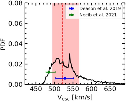
The posterior distribution of the escaped velocity at the solar position for the Zhao DM density model. The red-dashed line and shaded region indicate the median and 68 percentiles for the distribution, and these values are listed in Table 2.
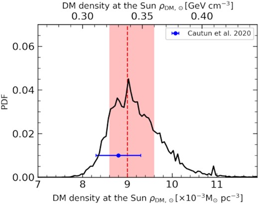
The distribution of DM density at the solar position for the Spheroid model. The median and associated 68 percentile of the posterior distribution from our MCMC runs are indicated by red-dashed line and shaded regions, and these values are listed in Table 2.
6 DISCUSSION
6.1 Influence of the a priori choice of the MW mass density profile
The MW baryon content is relatively well known, though there are still variations by ∼30 per cent for each component from one study to another (see Pouliasis, Di Matteo & Haywood 2017). Our method recovers these uncertainties by letting varying by similar amount the baryonic components.
The DM content of the MW is less constrained since it is found highly dependent on the choice of tracers. Here, we have used very robust tracers, which are stars embedded into the disc and GCs, as well as constraints from the vertical force. For the later, we even consider in Appendix A the alternative for which some (Crater) could be dwarf galaxy instead, or not bound (Pyxis). Our goal is to keep as large as possible the range of DM profile for the halo. This is why we have chosen both Zhao and Einasto profiles. The first one is a generalization of the NFW and of the generalized NFW profiles that have been often used to fit DM haloes. The second is acknowledged to reproduce better the DM halo density profile coming from simulations (Navarro et al. 2004; Gao et al. 2008; Dutton & Macciò 2014). It has also the advantage to be parametrized by only three parameters against five of the Zhao profile; however, it may become a disadvantage if more complex DM distribution is required, for e.g. fitting the MW mass profile in presence of a massive LMC.
Jiao et al. (2021) have shown that NFW and of the generalized NFW DM profiles may be biased in favour of high values for the total MW mass when compared to results using the Einasto profile. Results of our paper based on the Zhao’s DM profile indeed provide higher mass values than that from Einasto DM profile, which may confirm the Jiao et al. (2021) results. Nevertheless, we prefer to keep the whole range of possibilities in fitting the DM component of the MW, and to consider the whole range of MW masses provided by these two kinds of excellent models in reproducing the DM.
A recent study shows that the DM profile could be changed during the process of the baryon contraction in the centre region, which result in profile deviate from NFW (Cautun et al. 2020). We do not think this can alter our conclusions, because Jiao et al. (2021) showed that the Einasto model is able to reproduce a contracting halo.
6.2 A massive LMC may introduce disequilibrium
There have been many clues that a massive LMC ∼1011 M⊙ passing by MW could have non-negligible effects on the MW (Erkal, Belokurov & Parkin 2020; Petersen & Peñarrubia 2020; Conroy et al. 2021), and on the track of stellar streams (Erkal et al. 2019; Koposov et al. 2019; Vasiliev et al. 2021). For example, several halo tracers have shown velocity gradients that are predicted by a massive LMC model (Petersen & Peñarrubia 2020).
However, the fact that the LMC could be very massive is still under discussion. For example, GC distributions show no significant velocity shift (Erkal et al. 2020). Conroy et al. (2021) found that halo K giants show a local wake and a Northern overdensity, which can be explained by the passage of a massive LMC. However, as they showed a reasonable tilted triaxial halo model can explain this phenomenon equally well. It has often been acknowledged that the LMC is at first-passage to the MW (Kallivayalil et al. 2013). The splendid Magellanic Stream has been well reproduced under the frame of ‘ram-pressure plus collision’ model (Hammer et al. 2015; Wang et al. 2019), which reproduces well the neutral gas morphology including its structure into two filaments, the observed hot ionized distribution, as well as the very peculiar stellar morphology of the SMC. This model requires the total mass of LMC to be less than 2 × 10¹⁰ M⊙, which is almost one decade smaller than that of a very massive LMC.
To test the effect of LMC on the final MW mass measurement, we make a simulation to test how a massive LMC passing by MW may affect mass estimates. We follow the same method of Vasiliev et al. (2021) and we have built the pair of MW and LMC. Vasiliev et al. (2021) built models of the MW and LMC interaction to investigate the effect on the Sagittarius stream track. Their MW model consists of a stellar disc, bulge, and DM halo. The DM halo has axis-symmetric or triaxial-symmetric shape. For simplicity, we have used a spherical DM model. We also introduce a light gas component, which does not produce an essential effect on the total mass profile, but that is used to generate test particles for reproducing the modelled RC. The LMC has a truncated NFW profile with total mass 1.5 × 10¹¹ M⊙. We notice that the model of Vasiliev et al (2021) does not reproduce the MW RC (Eilers et al. 2019) and that it overestimates rotational velocities by about 5 per cent. We then slightly scale down the MW mass value to match the RC. We note that these small changes have little effects on the final results. We also remark that this modelling does not intent to reproduce whole full properties of the MW and massive LMC. Instead, its goal is to gauge the effect of a massive LMC to the constraints from the MW RC. Details on the structure of the pairs of LMC and MW and on the simulations of their interactions can be found in Vasiliev et al. (2021).
The LMC starts from 427 kpc away and is launched to reach the current observed position, at about 50 kpc to the MW centre. The top row of Fig. 11 shows the final velocity vector map of MW DM particles. The massive LMC induces a strong disequilibrium for MW system in which the systematic velocities are changed at different positions, which indicates that correcting the systematic effect is complex.
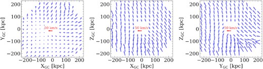
The simulated velocity vector maps for DM halo particles at different positions after the perturbation of a massive LMC (1.5 × 10¹¹ M⊙) passing by. Only particles outside the disc region (r >20 kpc) are shown.
Bearing in mind that the GC system shows no systematic velocity shift (Erkal et al. 2020), we build a mock observational sample from the simulated samples (Fig. 11). We randomly select the mock GC sample by using DM halo particles, adjusting their number to that of GCs.
With the simulated (mock) GC samples, we have perturbed the true value (|$s, v_{\mathrm{los}}, \mu _\alpha ^{*}, \mu _\delta$|) according to the uncertainties of the observed GCs. The distance uncertainty is |$\sim 5{{\ \rm per\ cent}}$|. The mean errors of line-of-sight velocity of the GCs are very small and fixed to 1.8 km s−1. The mean proper motion errors in both directions are ∼0.03 mas yr−1. The covariance correlation coefficiency are set by a randomly selected from Gaussian distribution with σ = 0.06 and zero mean value following observations.
To mimic the observed RC of Eilers et al. (2019), we have used the mean streaming velocity of gas particle, which has less velocity dispersion, and then less asymmetric drift correction. We also measured the vertical force at 1.1 kpc above the disc, which mimics the observation data (Bovy & Rix 2013). The RC and vertical force data in the simulated model have similar fraction errors as observations.
With the mimicked observation data in hand, we have used the action-based DF method listed above to model the gravitational field on the simulated data. Fig. 12 compares the final result to the true values. The green dashed line shows the true RC of input MW without LMC perturbation. The blue dashed line indicates the RC derived with V|$_c=\sqrt{\frac{GM(\lt r)}{r}}$| assuming a spherical mass distribution for the overall contribution of MW and LMC. The black-dashed line indicates the RC derived with |$\sqrt{R\frac{\partial {\Phi }}{\partial {R}}}$|. The mass estimate with the spherical mass distribution assumption is less accurate, because of the non-spherical shape of disc mass distribution and of the LMC contribution. The red-dashed line shows the results with action-based DF modelling. The contribution from the massive LMC is well recovered by the action-based PDF modelling, as shown by the slight bump of RC at ∼50 kpc in Fig. 12. The introduction of a massive LMC leads to overestimate the mass at large radius (r > 100 kpc). The black and cyan symbols show the gas streaming velocity in the centre region for both without and with LMC perturbation, both of these rotation velocities are consistent with each other. This indicates that the central region within the disc is much less affected by the massive LMC than the outer halo region, which provides us further confidence in using of RC data from Eilers et al. (2019).
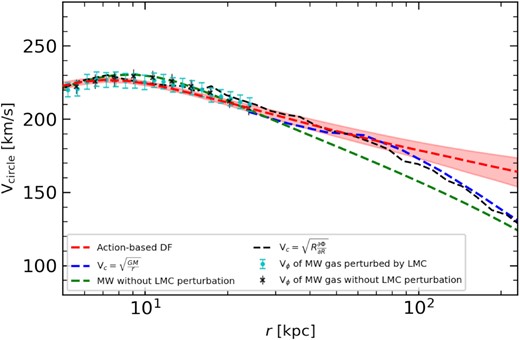
It compares the measured RC for the simulated GCs with observed values. The green-dashed line shows the input RC of MW without LMC perturbation. The blue-dashed line shows the RC for the MW perturbed by LMC calculated with V|$_c=\sqrt{\frac{GM(\lt r)}{r}}$|, which include the contribution by LMC. The black crosses show the measured streaming velocity of gas without LMC perturbation. The cyan dots show the streaming velocity of gas disc after LMC perturbation. The red-dash line shows the RC recovered by the action-based distribution method with shaded region indicate 68 per cent credible regions. The black-dashed line indicates the RC derived with |${\sqrt{R\frac{\partial {\Phi }}{\partial {R}}}}$| after LMC perturbation.
6.3 Effect of substructures
A recent discovery shows that the MW halo consists of many substructures, for example, the Sagittarius streams that contribute large fraction of halo stars (10 ∼ 15 per cent; Deason, Belokurov & Sanders 2019b; Deason et al. 2021). The big merger event, Gaia Sausage or Gaia Enceladus, which occurred 10 Gyr ago also contributes to a large fraction of inner halo stars (Belokurov et al. 2018; Helmi et al. 2018; Naidu et al. 2021).
In order to test the effect of these unrelaxed substructure effect on the measurement, we use the model m12m of the FIRE2 Latte cosmological hydrodynamic simulations suite, which produces a realistic MW-like galaxy, including many unrelaxed substructures (Hopkins 2015; Wetzel et al. 2016; Hopkins et al. 2018). From this model, we generate the mock GC sample. We select stars from model ‘m12m’ with age older than 10 Gyr, using them to represent the GC samples. From the simulated model, we derive the RC and vertical force at 1.1 kpc and add observational errors as in Hattori et al. (2021). With our modelling machine, we derive the final RC and compare it with input data as shown in Fig. 13. The unrelaxed substructures in the halo result only in moderate fluctuations of the RC.
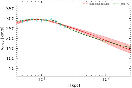
Comparing modelling results with mock MW-like of model ‘m12m’ of FIRE2, which is an MW-like galaxy from cosmological hydrodynamic simulations with unrelaxed substructures. The green-dashed line indicates the true RC for the model ‘m12m’, while the cyan points show the RC data with random errors added following observational errors. The red-dashed line and pink shaded region denote the modelling results and 68 per cent credible region from the models of MCMC run.
6.4 MW total mass and comparison with literature and implication for cosmology
The total mass is critical for many cosmological satellite problem, for instance, ‘too-big-to-fail’ (Boylan-Kolchin et al. 2011; Wang et al. 2012), and missing satellite problem. Our measurement for the mass of the MW is |$7.84_{-1.97}^{+3.08} \times 10^{11}$| M⊙ and |$5.8_{-0.68}^{+0.81}\times 10^{11}$| M⊙, after using the Zhao and the Einasto model for DM, respectively. Appendix discusses how these values can be slightly affected by different ways in using the GC sample, i.e. by removing or not Crater and Pyxis.
Fig. 14 compares the total MW mass measured in this work with recent results by using Gaia DR2 and EDR3. This figure is an update of fig. 5 of Wang et al. (2020), in which the results are grouped on the basis of the different methods used to estimate the MW total mass. Our range of estimates is at the low end of MW mass, which may alleviate the tension of the ‘too-big-to fail’ problem. Recent studies have suggested that only three MW satellites (MCs and Sagittarius dwarf; see Wang et al. 2012) could inhabit in sub-haloes with their value of Vmax larger than a threshold Vth ∼ 30 km s−1, which is defined by Boylan-Kolchin et al. (2011) as the massive failure threshold. Wang et al. (2012) used ΛCDM cosmological simulations and showed that only ∼5 per cent of haloes with mass Mhalo ∼ 2 × 10¹² M⊙ have three or fewer sub-haloes with Vmax > 30 km s−1, while this fraction increases to ∼70 per cent for an MW mass of 7.5 × 10¹¹ M⊙. The total mass of MW in our measurement naturally includes the contribution for LMC in our measurement, since the contribution by LMC has been added into the measured velocity for GCs. By assuming the LMC mass is 1.5 × 10¹¹ M⊙, leads to an MW total mass of 6.34 × 10¹¹ M⊙.
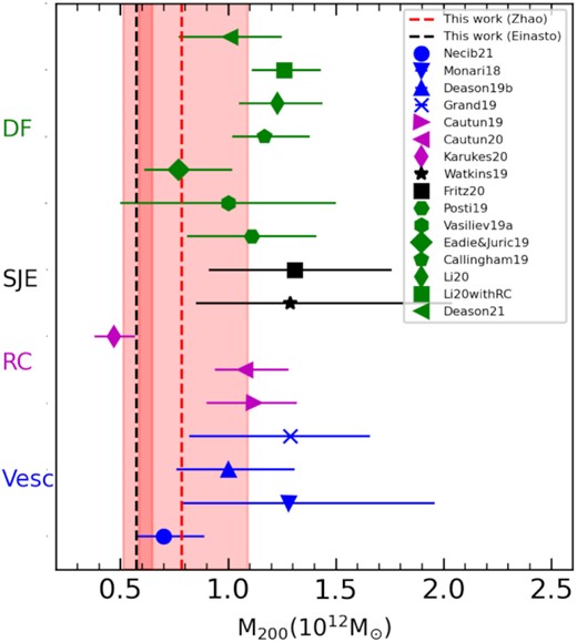
Comparing MW total mass results measured in this work with that made use of Gaia DR2 or EDR3. This figure is an update of Fig. 5 in Wang et al. (2020). Different methods have been labelled with different colour. DF (distribution function): Posti & Helmi (2019), Vasiliev (2019b), Eadie & Jurić (2019), Callingham et al. (2019), Li et al. (2020), Deason et al. (2021), Spherical Jeans Equation (SJE): Watkins et al. (2019), Fritz et al. (2020), RC: Karukes et al. (2020), Cautun et al. (2019, 2020), Escaped Velocity (Vesc): Necib & Lin (2021), Monari et al. (2018), Deason et al. (2019a), Grand et al. (2019). Red-dashed line indicates result of this work for Zhao’s DM profile, and black-dashed line shows result from Einasto’s DM profile. The pink shaded region shows the 68 percentile credible intervals.
7 CONCLUSION
Using Gaia EDR3 data, we derive proper motions for about 150 MW GCs. When comparing their proper motions with that from Gaia DR2, errors decrease by about a factor 2, which is consistent with the Gaia data reduction analysis.
With the newly derived proper motions for the MW GCs and by combining them to the constraints from the RC from 5 to 25 kpc and from the vertical force measurements, we have built dynamical models for the MW using the action-based distribution function. From the new dynamical model, we have derived the RC and the mass profile for MW, and have compared them with recent results based on Gaia data. The local DM density and local escaped velocity are all consistent with literature values.
We have used mock simulation data to test the robustness of our results. First, we consider the perturbation of a possible massive LMC passing by MW, which results in the reflex motion of halo stars with velocity intensities and directions modified at different positions (Fig. 11). By modelling mock GCs system from the simulations with action-based DF and comparing with the input value, we found the modelling can well recover the input RC value including the contribution from the massive LMC (1.5 × 10¹¹ M⊙) within 100 kpc. At large distances, this model overestimates the RC ∼20 per cent at 200 kpc. Secondly, we consider the effect of unrelaxed substructures on the results. We have used the realistic cosmological hydrodynamic simulations from FIRE2 Latter simulation data suite. The model ‘m12m’ produce an MW-like galaxy with unrelaxed substructures. From the data model, we select stars with age older than 10 Gyr to build mock GCs system. The unrelaxed substructure results in the final RC fluctuating around its true value by about 10 per cent.
In this paper, we have chosen the most objective view in adopting baryonic and DM mass, by avoiding a priori against or for a given modelling. It results that the total mass of the MW ranges from |$5.36_{-0.68}^{+0.81}\times 10^{11}$| M⊙ to |$7.84_{-1.97}^{+3.08} \times 10^{11}$| M⊙, which significantly narrows the previous ranges for the MW mass in the literature.
ACKNOWLEDGEMENTS
We thank the referee for helpful comments, which have significantly improved the manuscript. The computing task was carried out on the HPC cluster at China National Astronomical Data Center (NADC). NADC is a National Science and Technology Innovation Base hosted at National Astronomical Observatories, Chinese Academy of Sciences. This work is supported by Grant No. 12073047 of the National Natural Science Foundation of China.
This work has made use of data from the European Space Agency (ESA) mission Gaia (http://www.cosmos.esa.int/gaia), processed by the Gaia Data Processing and Analysis Consortium (DPAC, http://www.cosmos.esa.int/web/gaia/dpac/consortium). Funding for the DPAC has been provided by national institutions, in particular the institutions participating in the Gaia Multilateral Agreement.
DATA AVAILABILITY
The data underlying this article will be shared on reasonable request to the corresponding author.
REFERENCES
APPENDIX A: DYNAMICAL MODELLING ON GCS WITH EINASTO PROFILE
Fig. A1 shows the result of the dynamical modelling of the GC system based on the Einasto DM profile (equation 7). The Einasto DM profile results in a lower mass estimate at r > 100 kpc compared to that from Zhao’s DM profile (Fig. 8). Figs A2 and A3 show the posterior distribution for gravitational and DF parameters with Einasto’s DM profile.
It compares RCs derived from posterior distribution of our models with literature. Here, the Einasto DM profile is used. The shaded region indicates the 68 percentile.
Posterior distribution of parameters for potential fields with model using the Einasto’s DM density profile (equation 7). The parameters log ρ0, log rh, β, are for parameters of DM mass distribution. The parameters Mthin, Mthick, Mbulge are total mass for the thin and thick disc, and bulge components, and their units are 1010 M⊙. The parameters hthin, hthick indicate the scale length for thin and thick disc. The contour lines in each panel and the vertical lines in the marginal histograms are shown the 16 per cent, 50 per cent, 84 per cent percentiles.
Posterior distribution of parameters of DF (equation 8) of GCs with model using the Einasto’s DM density profile (equation 7). The parameters B and Γ related to the outer and inner slopes of DF, while η determines the steepness of transition. The dimensionless parameters gr, gz, hr, hz control the density shape and the velocity ellipsoid in the outer and inner region. The inner and outer regions are separated with actions J0. κ controls the rotation. The contour lines in each panel and the vertical lines in the marginal histograms show the 16 per cent, 50 per cent, 84 per cent percentiles.
We also notice that there are two GCs, Crater and Pyxis, for which properties are still disputed. It is not fully clear whether Crater is a dwarf or a GC (Bonifacio et al. 2015; Voggel et al. 2016), and Fritz et al. (2017) argued that Pyxis is accreted from a disrupted dwarf. We tested our results by excluding the two GCs from our samples, and found the MW total mass are |$6.77_{-1.74}^{+3.00}\times 10^{11}$| M⊙ and |$5.36_{-0.68}^{+0.81}\times 10^{11}$| M⊙ with Zhao and Einasto profile, respectively. These values are lower than those derived with the full samples (Table 2). We note that the multipopulation in the samples have no significant effect on our results as being test with our FIRE2 simulation. The proper motion of Pyxis in the Gaia DR2 and EDR3 (this work and Vasiliev 2019b; Vasiliev & Baumgardt 2021) is smaller than that used in Fritz et al. (2017), which corresponds to velocity decrease by ∼70 km s−1 and making Pyxis bound to the MW system. Therefore, including it in the samples is reasonable.
APPENDIX B: DYNAMICAL MODELLING ON GCS WITH DATA FROM VASILIEV ET AL. (2021)
In order to check how the results changing with PM results of Vasiliev & Baumgardt (2021), we also run our code on GCs data from Vasiliev & Baumgardt (2021) as shown in Fig. B1. The results are very similar to that with GC PMs derived in this work. The total mass of MW with the data of Vasiliev & Baumgardt (2021) is |$8.27_{-2.14}^{+3.59} \times 10^{11}$| M⊙, which is slightly larger than the result with our GCs data, but still within the error bars.
Comparing RCs derived from posterior distribution of our models with literature with GCs data from Vasiliev & Baumgardt (2021). Zhao’s DM profile is used. The shaded region indicates the 68 percentile.
