


ABSTRACT
As the statistical power of galaxy weak lensing reaches per cent level precision, large, realistic, and robust simulations are required to calibrate observational systematics, especially given the increased importance of object blending as survey depths increase. To capture the coupled effects of blending in both shear and photometric redshift calibration, we define the effective redshift distribution for lensing, nγ(z), and describe how to estimate it using image simulations. We use an extensive suite of tailored image simulations to characterize the performance of the shear estimation pipeline applied to the Dark Energy Survey (DES) Year 3 data set. We describe the multiband, multi-epoch simulations, and demonstrate their high level of realism through comparisons to the real DES data. We isolate the effects that generate shear calibration biases by running variations on our fiducial simulation, and find that blending-related effects are the dominant contribution to the mean multiplicative bias of approximately |$-2{{\ \rm per\ cent}}$|. By generating simulations with input shear signals that vary with redshift, we calibrate biases in our estimation of the effective redshift distribution, and demonstrate the importance of this approach when blending is present. We provide corrected effective redshift distributions that incorporate statistical and systematic uncertainties, ready for use in DES Year 3 weak lensing analyses.
1 INTRODUCTION
The most thoroughly studied biases in weak lensing measurements have mainly been performed with simulations of isolated objects. These include noise bias (e.g. Kacprzak et al. 2012; Refregier et al. 2012), model bias (e.g. Voigt & Bridle 2010), selection biases (e.g. Kaiser 2000; Bernstein & Jarvis 2002; Hirata & Seljak 2003), and biases from miscorrecting for the image point spread function (PSF; e.g. Paulin-Henriksson et al. 2008). These problems were tackled by community-driven efforts like the STEP (Heymans et al. 2006; Massey et al. 2007) and GREAT (Bridle et al. 2010; Kitching et al. 2013; Mandelbaum et al. 2015) challenges, and aided by the development of the widely used GalSim1 software for simulation of astronomical images (Rowe et al. 2015). For isolated objects, the aforementioned biases have largely been solved by methods like metacalibration (Huff & Mandelbaum 2017; Sheldon & Huff 2017) and ‘Bayesian Fourier Domain’ (BFD; Bernstein et al. 2016), at least for sufficiently well-understood data (i.e. with accurately characterized noise and background levels and PSF). The metacalibration method is particularly powerful because it does not rely on calibration simulations, which inevitably rely on assumptions about the properties of the faint, often poorly resolved galaxies used in weak lensing analyses.
More recently, some studies have begun to study shear calibration biases in the context of multiple objects and blending. It has generally been assumed that in this case the use of image simulations will be essential, and these have been used for the calibration of recent weak lensing cosmology analyses, for example by Fenech Conti et al. (2017), Kannawadi et al. (2019) (for the Kilo-Degree Survey2), Mandelbaum et al. (2018) (for the Hyper Suprime-Cam Subaru Strategic Program3), and Samuroff et al. (2018), Kacprzak et al. (2020) (for Dark Energy Survey, DES, Year 1 analyses). Works such as Hoekstra, Viola & Herbonnet (2017) and Euclid Collaboration (2019), with an eye to deeper upcoming data sets, have used image simulations to study effects such as the impact of undetected galaxies on the shear calibration.
In parallel to these simulation-based calibration efforts, Sheldon et al. (2020) developed new measurement methodology, metadetection, which corrects for much of the impact of blending, in particular the significant shear biases imparted by detection and deblending algorithms, as well as the impact of blending at the shape measurement stage. The metadetection method does not require simulation-based calibration, and exhibits extremely low levels of shear calibration bias even on (constant shear) simulations designed to match the depth of Rubin Observatory Legacy Survey of Space and Time4 (LSST) data.
Current and future surveys will have large amounts of blending of objects at different redshifts (e.g. Dawson et al. 2016). The component galaxies in blended systems will therefore often experience different shears. As we will discuss in Section 2, the impact of this on weak lensing statistics cannot be fully accounted for by the use of simplified constant shear simulations used thus far in the field to calibrate shear measurements, or corrections from shear estimation methods like metadetection. In order to gain intuition into the possible effects, consider the following simplified situation, shown in Fig. 1. In both panels, we input a pair of galaxies at different redshifts; for the sake of illustration we arbitrarily set one at low redshift (z = 0.25) and one at high redshift (z = 0.75). The high redshift galaxy is placed at the centre of the stamp in both panels. For simplicity, we have fixed both galaxies to be round before lensing. In the top panels, the galaxies are not blended together, and in the bottom panels they are. In both cases, we assume we can unambiguously detect two separate objects and precisely know their centroids.
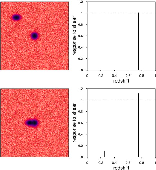
Simple example of the interplay between blending, shear calibration, and photometric redshift distributions. In both rows, the left-hand panel shows an image of a pair of simulated galaxies, with the central object at higher redshift, z = 0.75, and a neighbouring object at low redshift, z = 0.25. The right-hand panels show the response of the shape measurement of the central (z = 0.75) object, to applied shear, as a function of the redshift at which that shear is applied. In the top-row, where the objects are not blended, the high-redshift object only responds to a shear at its own redshift, and since we use metacalibration shear estimation, the response is unity (i.e. the shear estimation is unbiased) to very high precision. In the bottom right panel, we show the response when the objects are blended. We see two effects here. First, due to blending, the metacalibration estimator is now biased (the right peak at z = 0.75 has non-unit height). Secondly, the high-redshift object now responds to input shears at other redshifts (the small peak at z = 0.25). We show in this work that these responses define the effective redshift distribution for lensing predictions, in addition to quantifying the multiplicative bias of the measurements.
Let us consider the response to shear of the central (z = 0.75) object in each stamp. We can apply shear separately at the two redshifts from which the light in the image is sourced (which in this case just means applying shear separately to the two galaxies present in the stamp). The right-hand panels of Fig. 1 show the response to shear of the measured shape of the central galaxy, as a function of the redshift of the applied shear. The response is defined here as above, as |$R\, {=}\, {\scriptstyle \left(\partial \bar{g}^{\mathrm{obs}}/\partial g^{\mathrm{true}}\right)}$|. We estimated these responses numerically from our simple simulations using the metacalibration method. In the top right panel, we see that the high redshift object does not respond to the shear of the low redshift one (it is zero at z = 0.25) and has a unit response to a shear applied at its own redshift (the peak at z = 0.75). This result makes sense since metacalibration is known to be unbiased at high precision for idealized cases such as this, and the objects do not overlap.
The more interesting case is when the galaxies are blended, shown in the lower panels of Fig. 1. In this case, we see that the high redshift object responds to the shear of the low redshift object (the small peak at z = 0.25). It also has an apparent greater than unity response to the shear applied at its own redshift (the peak at z = 0.75 that is greater than one). Both of these effects are due to the galaxy being blended with the low redshift neighbour. The latter effect is likely due to the positioning of the neighbouring galaxy in the positive g1 direction, which is the shear component for which we compute the response.
However, the response of the high redshift object to a low redshift shear is a qualitatively different effect, distinct from standard multiplicative biases due to blending or detection; it is a bias that depends not only on the presence of the neighbour, but also on the shear applied to the neighbour. This indicates that the shape measurement of the high redshift object is carrying information about the low redshift shear.
In fact, we assert that it is the response to shear that defines how we should weight the redshifts to which we assign the shear information for a given object in a weak lensing analysis. This insight is a key subject of this work, where we will definitively measure these effects in simulations of the DES Year 3 (Y3) analysis (note that ‘Year 3’ includes the first three years of DES observations). There are also important implications for analysis of future surveys. As the amount of blending increases with increased depth, inferring the redshift distribution relevant for lensing and the shear calibration biases will be a joint analysis task. In the example above, we have described how a single detected object can have a (non-unity) response to shear at multiple redshifts. This effect cannot be fully described by the traditional multiplicative bias, m. The shear calibration and the effective redshift distribution cannot be fully decoupled.
In this work, we expand upon the ideas from this simple example and apply them to the DES Year 3 shear analysis. We introduce our formalism for accounting for blending in Section 2. In Section 3, we describe realistic simulations of the DES Year 3 survey, validating them against the data. Then in Section 4, we describe and investigate the source of the traditional shear calibration biases estimated from constant shear simulations. In Section 5, we show that the biases described above, due to blended sources with different applied shears, are present in these DES Y3 simulations. We then present a method to combine mean shear measurements from the simulations with estimated redshift distributions in order to jointly infer corrections to both the shear calibration and the redshift distributions. We apply this method to the DES Year 3 simulations, producing a parametrized model of these effects that can be used to interpret the DES Year 3 shear catalogues, which we describe in Section 6. We summarize and discuss directions for future work in Section 7.
2 QUANTIFYING SHEAR CALIBRATION BIASES FOR WEAK LENSING SHEAR STATISTICS
In the following, we describe our formalism and methodology of using image simulations to calibrate gravitational lensing measurements. To this end it is useful to distinguish galaxies from detections. We take a galaxy to be emitting light of fixed redshift z, with a particular surface brightness profile local to a position |$\boldsymbol {\theta }$| on the sky. A detection on the other hand is, simply put, a thing identified by an algorithm designed to detect and deblend astronomical sources, such as that employed by SExtractor (Bertin & Arnouts 1996). Due to blending, measurements made on a detection may be affected by light from multiple galaxies or stars and therefore multiple redshifts. We only have access to detections in an imaging survey, and we measure statistics averaged over ensembles of detections. We thus must determine how effects such as blending affect weak lensing shear statistics of ensembles of detections, rather than individual galaxies.
2.1 Isolated galaxies
2.2 Isolated galaxies with shear measurement biases
2.3 Blended galaxies and the general case
The definition of nγ(z) of equation (9) seems natural and has been used not only in DES Year 1 (Hoyle et al. 2018), but in some form by most other weak gravitational lensing analyses to date. It is accurate under the assumptions made – that each detection corresponds to light from a single redshift, and that while response to shear may be imperfect, it can be described by its mean as a function of the redshift, or estimated based on some properties of the images of actual detections, each associated with a single redshift.
Equations (13) and (14) constitute definitions of the effective redshift distribution that should be used to describe a sample of detections in a weak gravitational lensing analysis e.g. for predicting shear correlation functions or tangential shear signals. Note that the normalization of nγ(z), i.e. |$\int _0^\infty \mathrm{ d}z n_{\gamma }(z)$|, is now meaningful. The normalization is the response of the mean measured shear to a true shear that is constant in redshift. This corresponds to the traditional 1 + m, where m is the mean multiplicative bias for the ensemble. Note that numerical codes for making theoretical predictions of weak lensing statistics often internally normalize the provided redshift distribution. In this case, one would need to apply the normalization of nγ(z) to the predicted statistic as an additional correction.
The use of nγ(z) unifies two effects: biases in photometric redshifts and shear calibration, which have traditionally been treated separately. As we enter the era of deeper galaxy surveys, where blending becomes more and more important, we no longer have the luxury of treating these two systematic effects separately.
2.4 Calibrating nγ with image simulations
The definition of nγ(z) in equation (9) is superseded by that of equation (13). In the presence of blending, the two are expected to disagree, not just in their normalization (i.e. as an overall multiplicative bias), but also in their shape.
Photometric and/or clustering-based redshift calibration, can at best (when combined with a metacalibration response estimate for each detection) aim to measure |$\bar{R}(z)n(z)$|. Image simulations must be used to check whether the difference between |$\bar{R}(z)n(z)$| and the true nγ(z) is small, as one might hope as long as blending is rare or mild. In case that difference is not negligible, image simulation methods can be used to infer corrections to |$\bar{R}(z)n(z)$| that improve its agreement with the true nγ(z); this is the approach taken in Section 5 of this work.
Thus far, we have only considered a single ensemble of detections, and its effective redshift distribution for lensing, nγ(z). In Section 5, we will estimate these quantities for multiple subsets of our simulated detections, for example true or photometric redshift bins. In this case, we assign these subsets a label i, and denote as |$\bar{g}^{\mathrm{obs}}_i$|, nγ,i(z) and |$N_{\gamma ,i}^\alpha$|, the mean measured shear, effective redshift distribution and integrated effective redshift distribution for the subset i of our detections.
In the absence of blending, and if there were no overlap between the redshift interval α, and the redshift range of galaxies contributing to detections in subset i, |$\Delta \bar{\gamma }^{\text{obs}}_i$| and thus |$N_{\gamma ,i}^\alpha (z)$| would vanish i.e. there would be no response of the mean shear for subset i to shear in redshift interval α. Blending, however, causes a non-zero response for any realistic selection of an ensemble i of detections. This is because there will always be some amount of blending between galaxies in redshift interval α, and the detections in i, and shear applied to the former will impact the measurement of the shapes of the latter.
3 DES Y3 IMAGE SIMULATIONS
Having introduced and motivated our formalism for quantifying observational biases, we now turn to describing and validating our suite of DES Year 3-like image simulations. We note again here that DES Year 3 refers to the first three years of DES data processed together. In our simulation design, we follow closely the real DES Year 3 data, by simulating complete sets of single-epoch images required to form DES Year 3 tiles in all four photometric bands griz, and then applying the same software for coadding, object detection, and object measurement as is applied on the real data in Sevilla-Noarbe et al. (2021) and Gatti et al. (2021). This consistent simulation of weak lensing data across multiple photometric bands is key a step forward in the DES’s joint shear and photo-z bias characterization. We describe the main steps in our fiducial simulation pipeline below.
3.1 Exposures, single-epoch images, and tiles
DES wide-field images are processed in tiles, square sky regions of side length 10 000 pixel (≈0.72 degree, see Morganson et al. 2018). There are 10 338 such tiles included in the Y3 data set. For each tile region, all images overlapping that region are included in a coadded image for each band. These input images to the coadd come from many exposures, each of which is a collection of images, one for each CCD in the Dark Energy Camera (DECam; Flaugher et al. 2015) focal plane. We refer to these individual CCD images as single-epoch images. We also organize our image simulation using this tiling system.
We select at random 400 of the tiles entering the Y3 data set, and for each tile, generate simulated versions of all the single-epoch images with any overlap of the tile region. For a given version of our simulation, this constitutes 62.8 million simulated objects, of which 15.4 million are detected in our shear pipeline, and 4.1 million pass shear catalogue quality cuts (see Section 3.4). We simulate a total of 20 versions of this 400 tile set simulation, with versions differing only in their applied shear field (see Section 3.2), or whether objects are placed on a regular grid and whether detection is performed (see Section 3.5). We were limited in producing more simulation volume by time and computing resources, but find that this 400 tile set is sufficient volume such that statistical uncertainties in the simulation measurements are not the dominant uncertainty on our inferred bias corrections.
3.2 Single-epoch image generation
Our simulation pipeline starts by generating a simulated version of each single-epoch image using GalSim5 (Rowe et al. 2015), with the addition of various custom modules. Briefly, we create simulated images with noise, PSFs and world-coordinate system (WCS) estimated from the DES Y3 data, and insert parametric models for stars and galaxies. The images are simulated with the following properties:
Pixel geometry: Each simulated single-epoch image is generated with the pixel geometry of the corresponding image in the real DES data. This is simply set by the DECam CCD properties, all of which have 4096 × 2048 pixels.
Noise: Noise is assumed to be Gaussian and is drawn from the weight maps estimated for the corresponding image in the real DES data. For pixels that are masked in the corresponding image, the median of the weight map is used as the inverse noise variance. This noise field constitutes the only background on to which simulated objects are drawn – we do not simulate e.g. non-zero sky background. This choice implicitly assumes that the background subtraction performed on the Y3 data is sufficiently accurate.
WCS: Our input objects to the simulation, for which we generate a model in sky coordinates, are consistently drawn into all the single-epoch images they overlap, using the WCS (world-coordinate system) solution for the corresponding image in the real data.
PSF: The drawn objects are convolved with a smoothed version of the PSF model estimated from the real data by Piff6 (Jarvis et al. 2021). See Appendix C (Supplementary data) for the details and justification of this procedure. A significant simplification of our analysis here is that we do not attempt to measure the PSF from our simulations for use in shape measurement, rather we use the input PSF models. While we believe this is well justified by the stringent PSF validation performed in Jarvis et al. (2021), jointly simulating the inference of PSF and shear would be a natural extension of the work presented here.
Masking: We package with the simulated images the bad pixel masks taken from the corresponding real data image files. These indicate pixels to exclude or interpolate for downstream processing and measurement codes.
Input galaxies: We randomly draw galaxy models from a catalogue of ‘bulge + disc’, two-component parametric fits to galaxies in the COSMOS field.7 This catalogue is described in Hartley et al. (2020); we provide a brief description here. The morphological parameters (half-light-radius, bulge-to-disc-ratio, ellipticity) of the parametric galaxy models were fit to Hubble Space Telescope Advanced Camera for Surveys (HST-ACS) imaging (Koekemoer et al. 2007; Scoville et al. 2007), specifically we use the re-processed HST-ACS data of Leauthaud et al. (2007). These model fits were then used to estimate fluxes for the DECam griz filter bandpasses, using forced photometry at the same sky positions in deep stacks of DECam imaging (described in Hartley et al. 2020). The use of both HST imaging and DECam imaging gives us a catalogue of parametric galaxy models with realistic and well-constrained morphology (from HST) and realistic fluxes and colours in the DES filters (from the deep DES imaging). When drawing a parametric model galaxy into the simulations, we apply a random rotation to each simulated object.
We additionally match this catalogue (using a 0.75 arcsec matching radius) to the Laigle et al. (2016) redshift catalogue, and apply area masks for the problematic regions identified by Hartley et al. (2020), after which 222 116 unique input objects remain. We remove 60 (|$0.03{{\ \rm per\ cent}}$|) of these for which the parametric model fits failed. We additionally apply a selection r50 > −0.25(magi − 22) − 1.35, which we find effectively removes the stars (we separately simulate stars using a different catalogue described below).
In our fiducial simulation, we include only galaxies with i-band magnitude <25.5, which is two magnitudes fainter than our threshold for inclusion in the eventual shape catalogue. While we do not perform an analysis of sensitivity to this choice, the results of e.g. Hoekstra, Viola & Herbonnet (2017) suggest the absence of fainter objects than this in our simulations will probably bias our multiplicative bias estimates at the |$\sim 0.1{{\ \rm per\ cent}}$| level, well below our current uncertainties.
In each tile, the number of galaxies simulated is drawn from a Poisson distribution with mean 170 000, which corresponds to a number density of 88 galaxies per square arcmin. The density of input objects was tuned such that the number of detected objects in the simulations matched the number of detected objects for the same set of tiles in the real DES Y3 data. The majority of these galaxies will be either undetected or removed via cuts, resulting in a number density of roughly 6 galaxies per square arcmin used for shear estimation.
Galaxies are placed randomly on the sky and so are not clustered. Compared to the real Universe, we expect this to result in less blending of objects at similar redshifts. We discuss the implications of this approximation in Sections 6.3 and 7.
Input stars: We use a catalogue of stars simulated using the trilegal8 code, with the best-fitting models from the MWFitting method presented in Pieres et al. (2020). This catalogue contains both sky positions and fluxes for a simulated population of stars complete in the magnitude range 14–26 in the g-band. In our fiducial simulation, we include only stars with i-band magnitude <25.5.
Input shear: We run otherwise identical realizations of each simulation with constant input shears of either +0.02 or −0.02 in a single shear component (the other component being 0). This allows us to follow the approach of Pujol et al. (2019), who propose computing multiplicative shear biases via measuring the difference in recovered shear between two simulations that are identical apart from a small change in input shear. Using this procedure greatly reduces the noise (both shape noise and measurement noise) on the multiplicative bias estimate, since much of it cancels when taking the difference. Note this is closely related to the idea of the ‘ring-test’ introduced by Nakajima & Bernstein (2007). We additionally generate simulations where the applied shear depends on the redshift of the input galaxy. More specifically, we generate simulations where galaxies with redshift within some redshift interval α have a difference in applied shear of |$\Delta g^{\mathrm{true}}_{\alpha }= 0.04$| with respect to the rest of the simulated galaxies. This allows us to measure the |$N_{\gamma }^{\alpha }$| as described in Section 5.1.
3.3 Image reduction, coaddition, and detection
The processing and measurements applied to the simulated images closely follow that performed on the real DES Y3 images (described in Morganson et al. 2018; Gatti et al. 2021; Sevilla-Noarbe et al. 2021). We summarize here:
A 10 000 × 10 000 pixel weighted-mean coadd image is generated for each tile, in each band, using SWarp (Bertin et al. 2002). The weight maps used are the same as those used to generate the noise on the simulated images. The r, i, and z coadd images are then themselves combined in a CHI-MEAN coadd image, again using SWarp.
The riz coadd is used for object detection and segmentation, which is performed by SExtractor (Bertin & Arnouts 1996). SExtractor outputs a catalogue of detected objects, various measured quantities for these objects, as well as segmentation maps (which indicate which pixels in the images are assigned to which catalogue objects).
Multi-epoch data structure (MEDS; Jarvis et al. 2016) files are generated for each band for each tile. For each detected object in the SE xtractor catalogue, the MEDS file contains a postage-stamp cutout from each of the single-epoch images in which that object appears. This data format makes convenient the fitting of models simultaneously to multiple observations of a given object.
3.4 Shear estimation
To generate a shear catalogue for each tile, we run metacalibration on the r, i, and z MEDS files, which fits an elliptical Gaussian profile, convolved with the PSF model, to the observed light profile of each detection. The parameters of the profile are fit jointly to square regions (stamps) extracted from each single-epoch image for all bands, apart from a free amplitude allowing an independent flux in each band. Stamps with a masked fraction of more than 0.1 are not used in the fits. Estimates of the shear response, Rij are also generated by metacalibration which is the response of the measured shear in component i to an applied shear in component j. From the shear catalogues generated by metacalibration we select a sample suitable for weak lensing measurements by applying the identical catalogue cuts as those applied to the DES Y3 data in Gatti et al. (2021). The most significant (in terms of number of objects removed) of these are cuts on the object signal-to-noise ratio, S/N > 10, and the ratio of PSF-deconvolved galaxy size, T, to the PSF size, Tpsf, T/Tpsf > 0.5. T is an area measure (equal to the trace of the covariance) for the Gaussian profile. The signal-to-noise ratio cut is required to minimize biases associated with shear-dependence of the SExtractor selection, and the size cut reduces the impact of any PSF modelling errors. See Gatti et al. (2021) for more discussion of the motivation and details for the shear catalogue cuts, as well as detailed descriptions of the quantities such as T. This sample can then be used to estimate the shear recovered from the simulation, which can then be compared to the true shear input to the simulation to estimate any biases in the shear recovery.
3.5 Simulation variants
In order to better understand the source of shear calibration biases, we generate and analyse two sets of simulations additional to the fiducial simulation described thus far. In the grid simulations, objects are placed on a regular grid with spacing ≈35 pixels (≈9 arcsec). We would expect any biases related to blending to be absent in this variant. The second variant is the grid-truedet simulations, which again places objects on this regular grid, and in addition the SExtractor detection catalogue used as input to the shape measurement is replaced by a catalogue containing the true positions of input objects. We would expect this to remove any biases related to possible shear dependence of the SExtractor detection probability (e.g. if rounder objects were more likely to be detected).
3.6 Simulation validation
The final part of our simulation pipeline is validating our simulation’s realism by comparing it to the real data. We infer below that the shear biases present are related to the blending of sources and the possible shear-dependence in how sources are selected, segmented, and modelled. This blending must therefore be accurately characterized in the simulations. We ensure here that the number density of sources, the noise levels in the image, and the distribution of measured source properties like flux and size are well matched between the fiducial simulation and real DES data. We expect the effects of blending to be sensitive to the properties of neighbouring objects (such as the number of them within a given distance, and their brightness) encountered by our target source galaxies, so we additionally study statistics sensitive to these in Section 6.3.
3.6.1 Aesthetics
We generate gri colour images of our simulated coadds, using the desimage9 package. These are useful for visual inspection of the simulations, but also for visual comparison to images made via the same process on the real data. Fig. 2 shows colour images for the same 1000 × 1000 pixel region of the coadd tile DES0003-3832 in the real data (left-hand panel) and the fiducial simulation (right-hand panel). A lack of bright stars in the simulation is apparent. These are masked out of the real data before analysis, so we do not believe that their absence from the simulations can impact our results.
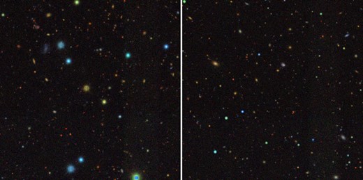
gri colour image of 1000 × 1000 pixel region of tile DES0003-3832 for the real Y3 data (left-hand panel) and the fiducial simulation (right-hand panel).
3.6.2 SExtractor comparisons
SExtractor forms a crucial part of our pipeline in detecting and segmenting objects in the coadd images, so it is important that the simulated images analysed using SExtractor resemble the real data. Here, we perform comparisons of the measured properties of objects detected in the simulations.
The top-left and top-middle panels of Fig. 3 show the joint distribution of magnitude and size estimated by SExtractor, for the g and i-bands, respectively. Specifically, we use MAG_AUTO (an elliptical aperture magnitude), and FLUX_RADIUS (with |${\tt PHOT_FLUXFRAC}=0.5$|) an estimate of the PSF-convolved half-light radius of the object.10 Some clear features are apparent in both simulations and data, such as the shift of the distribution to larger size in the g-band compared to the i-band, which is due primarily to the larger PSF. We note that the distributions plotted share the same normalization, so any differences in absolute number density would be apparent.
![Comparisons of joint distribution of measured quantities between simulations (orange dashed lines) and DES Y3 data (blue lines). The top-left and top-middle panels show joint distributions of SExtractor measured quantities MAG_AUTO and FLUX_RADIUS g-band and i-band, respectively. The stellar locus is at larger FLUX_RADIUS in the g-band because of the larger PSF. The remaining panels show comparison of quantities estimated by the shape measurement code (metacalibration). The top-right panel shows the joint distribution of signal-to-noise and size [in fact, log10(S/N) and log10(1 + T)]. The bottom-left panel shows the joint-distribution of i-band magnitude and r − i colour. The bottom-middle panel shows the joint distribution of i-band magnitude and i − z colour. The bottom-right panel shows the joint distribution of r − i and i − z colours.](https://oup.silverchair-cdn.com/oup/backfile/Content_public/Journal/mnras/509/3/10.1093_mnras_stab2870/1/m_stab2870fig3.jpeg?Expires=1749874354&Signature=Af3mSvBS4TRia933QtMiAsL11m0Hx82OldcopbfD0D7R-AsrcvC4STc8MbWXeK6lOSuFjGA5KGNkZ40EE-JiJEp0aqN9vcYZZvQuWcxYAejf6nWhj6qkvKN~Jl0MMgeTnh4eLjesqOc4gFSCzHZ4RTm8BBtN8RXp-AB-ZYBZasQ30nFFyEYCpj0dpp6UfNPV4O9ZTTg1xEjvoFJpttgh~n4UW8upLH8BjpBswx9ZXeNLyGj7BzluItmkvj7f6EMFGDID2UPr-uzQ5ouM0eVMp5t6fWf6-uIDuH0pnSBx64tpfZNe7MMCkJ0WxuC9enWJIjeX2pcCFaCX4SKyEypMEQ__&Key-Pair-Id=APKAIE5G5CRDK6RD3PGA)
Comparisons of joint distribution of measured quantities between simulations (orange dashed lines) and DES Y3 data (blue lines). The top-left and top-middle panels show joint distributions of SExtractor measured quantities MAG_AUTO and FLUX_RADIUS g-band and i-band, respectively. The stellar locus is at larger FLUX_RADIUS in the g-band because of the larger PSF. The remaining panels show comparison of quantities estimated by the shape measurement code (metacalibration). The top-right panel shows the joint distribution of signal-to-noise and size [in fact, log10(S/N) and log10(1 + T)]. The bottom-left panel shows the joint-distribution of i-band magnitude and r − i colour. The bottom-middle panel shows the joint distribution of i-band magnitude and i − z colour. The bottom-right panel shows the joint distribution of r − i and i − z colours.
3.6.3 Metacalibration quantities
For shear estimation and photometry, we use elliptical Gaussian models fit to single-epoch images (as opposed to the coadds used for the SExtractor quantities discussed above). The distributions of size and signal-to-noise of a weak lensing galaxy sample have often been identified as key to the expected level of bias in the shear recovery (e.g. Kacprzak et al. 2012; Refregier et al. 2012). The top-right panel of Fig. 3 compares the joint distribution of signal-to-noise and size between simulations and data. The distributions are smoother in the log of these quantities, so we actually compare distributions of log10(S/N) and (since T can take slightly negative values) log10(1 + T).
As well as size and signal-to-noise, it is important to verify that other quantities used to select sub-samples of the source galaxies are well matched between simulations and data. A key example of this is selection of objects into bins based on their photometric redshift (photo-z henceforth). Photo-z algorithms usually use some discrete set of broad-band fluxes, with ratios of those fluxes (or differences in magnitudes), known as colours considered particularly informative for redshift estimation. The bottom three panels of Fig. 3 demonstrate that the simulations reproduce well the joint distributions of (from left to right): i-band magnitude and r − i colour, i-band magnitude and i − z colour, and r − i colour and i − z colour.
3.7 Photo-z inference
The photometric redshift distributions for the simulation sample are inferred using the SOMPZ method outlined in Myles et al. (2021) (see also Buchs et al. 2019). Following the methodology applied to DES Y3 data there, detected objects in the image simulations are assigned to two self organizing maps (SOMs), corresponding to ‘wide’ (32 × 32 cells, using riz flux information) and ‘deep’ (64 × 64 cells, using ugrizJHKs colour information from the DES Deep Fields measurements presented in Hartley et al. 2020). In the Y3 data analysis, galaxies with spectroscopic redshifts or flux measurements in a large number of photometric bands (‘deep’ galaxies) are assigned to the higher resolution SOM. When those same galaxies are assigned to the lower resolution SOM based on their wide field flux information, they can be used to infer information about other galaxies with only the limited wide-field photometry available in order to calibrate the colour–redshift relation.
We use the SOMs constructed from the Y3 data catalogues and the same software to assign the simulated galaxies (Myles et al. 2021). We assume that all simulation input galaxies have precise redshifts (equal to the photo-z point estimates by Laigle et al. 2016) that, together with their measured deep ugrizJHKs fluxes, describe the deep colour–redshift relation. Matching simulation detections to input galaxies allows us to generate a transfer function that connects redshift, deep SOM cell, and wide SOM cell. The wide cells and their contained galaxies are then grouped together by their mean redshift in a variety of ways (see below) to form tomographic bins.
The procedure for matching injection galaxies to measured detections in these simulations begins with a nearest neighbours search to identify the three closest objects in the truth catalogue to a given detection. For a detection to be matched to a true object, it must have a close match within two pixels. If it does not have one, it is ignored in the rest of the photo-z inference (roughly |$0.5{{\ \rm per\ cent}}$| of detections). Detections with an exclusive close match (i.e. one that is not a close match to any other detection) make up approximately |$30{{\ \rm per\ cent}}$| of the simulated sample. To discriminate between detections with multiple close truth matches, we loop over injections from brightest to faintest in i-band magnitude and assign the brightest close truth match that has not yet been assigned to another detection. Roughly |$70{{\ \rm per\ cent}}$| of detections fall into this category. If all close matches have already been assigned to other detections via this loop, no truth match is assigned, but this happens rarely enough to be negligible. For example, this only occurs for four cases in the entire fiducial (g1, g2) = (−0.02, 0.00) simulation.
The wide SOM occupancy for both the simulations and the data can be seen in Fig. 4, showing very good general agreement. This is a consequence of the close alignment of colour and magnitude distributions between the data and the simulations discussed in Section 3.6.2. The largest point of discrepancy is due to cells composed of very large, very blue galaxies at low redshifts, which likely do not significantly contribute to the redshift-dependent effects of blending that are key to this analysis.
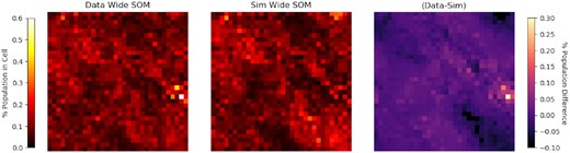
The wide SOM population distribution in the data (left) compared to the simulations (centre), with a residual (right) that shows the majority of cells agree to within 0.05 per cent in total population.
A principal aim of this work is to quantify the shear calibration separately for each of the photometric redshift bins used in the DES Y3 cosmology analyses. This requires that we perform an equivalent photometric redshift binning on the image simulations. One can motivate several different choices of photo-z binning algorithms in order to estimate the shear calibration biases that may differ due to the small differences in colour–redshift relation between the sims and the data. Presented here is a description of the four binning algorithms we use and their resulting summary statistics like the mean redshift per bin.
Fiducial: We use the same mapping between wide SOM cell and photo-z bin as in the Y3 data. We make this our fiducial choice, since we think the philosophy of treating the real data and the simulations as similarly as possible is a sensible one. However, small differences in wide SOM occupancy between simulations and real data are apparent with this procedure. Whereas in the data, each photo-z bin has an equal number of objects (25 per cent of the total, by construction), there are deviations from 25 per cent occupancy in the simulations, with the four photo-z bins receiving 19 per cent, 24 per cent, 25 per cent, and 30 per cent of the objects, respectively.
Equal count (equal): Instead of taking the mapping from the data, the wide SOM cells are ordered by mean redshift and then grouped such that an approximately equal number of galaxies end up in each photo-z bin, much like how the mapping is chosen in the data.
Mean redshift matching (z-match): This is a binning that chooses the wide SOM cells such that they closely match the mean redshift found in the data photo-z bins, with approximately equal counts in each bin. By necessity, in this binning scheme a galaxy may end up assigned to multiple bins, or not assigned to any bin.
SOM occupancy matching (w-match): This preserves the mapping used in the fiducial case, but also re-weights galaxies to reproduce the relative wide SOM cell occupancy found in the Y3 data, using the ratio between the left and centre panels of Fig. 4.
The mean redshift for each of these photo-z binning choices on the simulations is reported in Table 1, and the full distributions can be seen in Fig. 5. We see broad similarity between the binning recipes, but revisit the alternative options in Section 6.2 where we test the sensitivity of our calibration corrections to the choice of binning recipe.
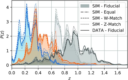
The photometric redshift distributions for the four photo-z binning schemes applied in the simulations (described in Section 3.7), as well as the estimated Y3 data redshift distributions (labelled ‘DATA - Fiducial’). For plotting purposes all curves have been smoothed using a Gaussian kernel of width 0.01 in z.
Table describing the mean redshift per photo-z bin for each binning algorithm as compared to that found in the data.
| Sample | Binning style | |$\bar{z}_0$| | |$\bar{z}_1$| | |$\bar{z}_2$| | |$\bar{z}_3$| |
|---|---|---|---|---|---|
| Data | Fiducial | 0.334 | 0.517 | 0.749 | 0.936 |
| Sim | Fiducial | 0.311 | 0.460 | 0.723 | 0.894 |
| Sim | Equal | 0.322 | 0.510 | 0.745 | 0.920 |
| Sim | Z-Match | 0.325 | 0.511 | 0.753 | 0.930 |
| Sim | W-Match | 0.294 | 0.463 | 0.714 | 0.895 |
4 RESULTS I: SHEAR CALIBRATION BIASES FROM CONSTANT SHEAR SIMULATIONS
In this section, we begin by examining the shear calibration biases apparent in constant shear simulations, and we report average shear calibration bias estimates for the full DES Y3-like sample, as well as for individual photo-z bins. As described in Section 2, these bias estimates are not sufficient in general to correct theoretical predictions for weak lensing shear statistics, hence in Section 5, we present estimates of biases in nγ(z), using simulations where the input shear varies with redshift.
Image simulation properties. Each line lists a specific image simulation produced for this work. The fiducial simulation places objects at random into the image and uses SExtractor for object detection. We also ran variations for some of the simulations where objects were placed on a grid (grid) or we used their true locations for shear measurements (grid-truedet).
| Variant | Sheared redshift interval | (g1, g2) in redshift interval | (g1, g2) outside redshift interval | Object placement | SE xtractor detection |
|---|---|---|---|---|---|
| grid-truedet | [0.0, 3.0] | (+ 0.02, 0.00) | – | grid | no |
| grid-truedet | [0.0, 3.0] | (− 0.02, 0.00) | – | grid | no |
| grid-truedet | [0.0, 3.0] | (0.00, +0.02) | – | grid | no |
| grid-truedet | [0.0, 3.0] | (0.00, −0.02) | – | grid | no |
| grid | [0.0, 3.0] | (+ 0.02, 0.00) | – | grid | yes |
| grid | [0.0, 3.0] | (− 0.02, 0.00) | – | grid | yes |
| grid | [0.0, 3.0] | (0.00, +0.02) | – | grid | yes |
| grid | [0.0, 3.0] | (0.00, −0.02) | – | grid | yes |
| fiducial | [0.0, 3.0] | (+ 0.02, 0.00) | – | random | yes |
| fiducial | [0.0, 3.0] | (− 0.02, 0.00) | – | random | yes |
| fiducial | [0.0, 3.0] | (0.00, +0.02) | – | random | yes |
| fiducial | [0.0, 3.0] | (0.00, −0.02) | – | random | yes |
| fiducial | [0.0, 0.4] | (+ 0.02, 0.00) | (− 0.02, 0.00) | random | yes |
| fiducial | [0.4, 0.7] | (+ 0.02, 0.00) | (− 0.02, 0.00) | random | yes |
| fiducial | [0.7, 1.0] | (+ 0.02, 0.00) | (− 0.02, 0.00) | random | yes |
| fiducial | [1.0, 3.0] | (+ 0.02, 0.00) | (− 0.02, 0.00) | random | yes |
| fiducial | [0.0, 0.4] | (0.00, +0.02) | (0.00, −0.02) | random | yes |
| fiducial | [0.4, 0.7] | (0.00, +0.02) | (0.00, −0.02) | random | yes |
| fiducial | [0.7, 1.0] | (0.00, +0.02) | (0.00, −0.02) | random | yes |
| fiducial | [1.0, 3.0] | (0.00, +0.02) | (0.00, −0.02) | random | yes |
Table 3 contains mean multiplicative biases for our fiducial, grid, and grid-truedet simulations. In the grid simulation, blending is removed by placing down objects on a grid. In the grid-truedet simulation, objects are again placed on a grid, and in addition we use their true positions for the detection catalogue, rather than the detection catalogue estimated using SExtractor. We expect this to additionally remove any selection biases due to shear-dependence of the SExtractor selection.
Average multiplicative (m) and additive (c) biases for the fiducial, grid, and grid-truedet simulations. While we expect no bias in the shear measurements for simulations of objects on a grid with no detection employed, we do find a small bias due to masking corrections. See Appendix B (Supplementary data) for details. The fiducial simulations show non-trivial multiplicative biases due to a combination of blending, object detection effects, masking, and potentially other unknown causes.
| Variant | m1 × 100 | m2 × 100 | m × 100 | c1 × 104 | c2 × 104 |
|---|---|---|---|---|---|
| grid-truedet | −0.48 ± 0.07 | −0.40 ± 0.07 | −0.44 ± 0.05 | −2.06 ± 1.48 | −2.77 ± 1.46 |
| grid | −0.33 ± 0.15 | −0.35 ± 0.15 | −0.34 ± 0.11 | −2.14 ± 1.34 | −3.59 ± 1.40 |
| fiducial | −2.23 ± 0.16 | −1.93 ± 0.17 | −2.08 ± 0.12 | −0.86 ± 1.35 | −1.34 ± 1.45 |
| fiducial bin 0 | −1.55 ± 0.44 | −0.96 ± 0.45 | −1.25 ± 0.31 | 1.57 ± 3.05 | −4.38 ± 2.75 |
| fiducial bin 1 | −1.77 ± 0.56 | −1.87 ± 0.54 | −1.82 ± 0.39 | −1.86 ± 2.66 | −0.69 ± 2.79 |
| fiducial bin 2 | −2.51 ± 0.64 | −2.03 ± 0.67 | −2.27 ± 0.44 | −3.05 ± 2.39 | 1.11 ± 2.43 |
| fiducial bin 3 | −0.038 ± 0.79 | −0.034 ± 0.88 | −3.60 ± 0.59 | 0.31 ± 2.78 | −1.24 ± 2.89 |
While the fiducial simulations exhibit a mean multiplicative bias of |$\approx -2{{\ \rm per\ cent}}$|, the multiplicative bias for both the grid and the grid-truedet simulations are greatly reduced, with a remaining bias of around |$-0.4{{\ \rm per\ cent}}$|. We can draw a few conclusions from this. First, the fact that we see consistent biases for the grid and grid-truedet cases implies that we do not have significant SExtractor biases for isolated objects. This is not unexpected, since we apply an S/N > 10 cut to our catalogues that likely dominates over the threshold for detection used by SExtractor, and Metacalibration is able to accurately correct for selection biases due to this cut.
Beyond that, we can attribute most of the multiplicative bias we see in the fiducial simulation to the presence of blending. As explored in Sheldon et al. (2020), the presence of blending can likely generate biases through various (related) mechanisms. First, there is ‘detection’ bias due to shear-dependence of the detection algorithm, including the decision of how many different objects to assign to a blend. Secondly, one may also expect an additional bias due to the presence of a neighbour in the shape measurement process, either due to its contaminating flux, or due to some unaccounted-for shear dependence of the neighbour masking algorithm. With these simulations, we cannot fully decouple these effects. A simulation with randomly placed objects as in the fiducial simulation, but using true detection to remove detection biases, would shed light on the issue, but we did not have the resources to run this variation.
Fig. 6 shows the multiplicative bias (averaged over shear component) as a function of signal-to-noise ratio. For the grid and grid-truedet cases, there is no clear trend with S/N, while for the fiducial case, there do appear to be variations with S/N, although only at the per cent level, and we do not attempt to explain this behaviour. We also do not have a conclusive explanation for the |$\approx -0.4{{\ \rm per\ cent}}$| biases remaining in the grid and grid-truedet simulations. Appendix B (Supplementary data) explores various potential sources of small (sub-per cent) multiplicative biases using idealized simulations, and we do see the potential for biases due to masking at the |$\sim 0.1{{\ \rm per\ cent}}$|, so this may be contributing some of the remaining bias. Given that we directly apply the masks from the DES Y3 data to our simulations, we are confident that the biases in the simulations due to masking will be at a similar level to that present in the real data.
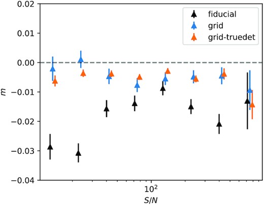
Multiplicative bias as a function of S/N for the fiducial, grid, and grid-truedet simulations. The fiducial simulation places the objects in the images at random positions and detects them with SExtractor. The grid simulation places them on a grid with ≈9 arcsec spacing and still employs SExtractor. The grid-truedet simulation uses a grid for the objects, but uses their true positions instead of detecting them with SExtractor.
In order to provide some more detail on the impact of blending on the multiplicative bias, we attempt to compute the bias as a function of object separation as follows. Using the galaxies in the input truth catalogues for our simulations, we find pairs of input galaxies that are separated by some distance and are no closer to any other galaxy in the simulation than the other galaxy in its pair. We then define a small region in the simulated image encompassing each pair, such that detections in this region include light from just these two galaxies. Specifically, we used a circle of radius 0.75 times the pair separation, centred on the midpoint between the two galaxies. Detections in these regions were used to compute the multiplicative bias as a function of separation. The results of this exercise are shown in Fig. 7. For comparison, we show the predicted effects of detection bias from Sheldon et al. (2020) for a simplified simulation set-up involving only pairs of galaxies with equal size and flux. Note also that Sheldon et al. (2020) used a different procedure to remove the light of neighbouring objects. At small separations, we see the qualitative effects of detection bias, which is a large negative bias. At large separations, the bias is consistent with zero within the statistical noise. At intermediate scales, we also see a positive bias that was not apparent in the Sheldon et al. (2020) simulation results. This can occur when a neighbour is not detected, so may only be significant when pairs with widely disparate fluxes are included.
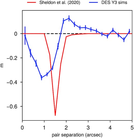
Multiplicative bias for detections corresponding to pairs of truth objects separated by a given angle. To make this plot, we find pairs of true objects separated by some distance in the truth catalogue in our fiducial simulations and not near any other objects. We then use detected objects near this location to measure the multiplicative bias as a function of separation. At small scales, we find signals in our simulations that appear to be from detection bias. For comparison, we show the detection bias result from Sheldon et al. (2020) as the red line. At intermediate scales, we see a positive bias, which is probably from pairs where one source is much fainter than the other. The bias converges to be consistent with zero at large separations.
To summarize, we see multiplicative biases in our simulations from at least three sources. First, as shown in Appendix B (Supplementary data), the effects of masking and their corrections used in the DES Y3 analysis cause a small, few tenths of a per cent bias. Secondly, for very close pairs of truth objects, we see a strong negative multiplicative bias in Fig. 7 that is qualitatively consistent with the detection biases studied in Sheldon et al. (2020). At intermediate separations, we see some positive multiplicative bias which is presumably blending-related, involving pairs with widely different fluxes.
We note here that the mean multiplicative bias of ≈−0.02 we estimate here is somewhat different from the multiplicative bias prior of 0.012 ± 0.012 inferred by Zuntz et al. (2018) for the DES Year 1 shear catalogue, which used very similar shape measurement methodology. We believe the significant improvements in simulation realism presented here explain this discrepancy. We note also that Sheldon et al. (2020), which used an independent set of image simulations to those presented here, that we believe also contained significant improvements with respect to those used by Zuntz et al. (2018), reported multiplicative biases much close to those presented here for DES-like simulations.
In Section 6.3, we use a re-weighting procedure to estimate systematic uncertainty (due to potential simulation inaccuracy) in the impact of blending, which is then propagated to our final priors on the shear calibration.
5 RESULTS II: ESTIMATES OF Nγ(Z) BIASES FROM REDSHIFT-DEPENDENT SHEAR SIMULATIONS
We explained in Section 2 that for theory predictions of shear statistics involving ensembles of detections over a range of redshifts, we require an estimate of nγ(z), the effective redshift distribution for lensing. In this section, we describe the extra simulations and methodology used to infer biases in the DES Y3 methodology for estimating nγ(z). To summarize, we take the following approach (with much more detail given in the following section). For each photo-z bin i:
We measure |$N_{\gamma ,i}^{\alpha }$| for four redshift intervals α (with ranges |$(z_1^\alpha ,z_2^\alpha)$|), from simulations with a change in applied shear within that interval. We use redshift intervals |$(z_1^\alpha ,z_2^\alpha) \in \lbrace (0.0,0.4),(0.4,0.7),(0.7,1.0),(1.0,3.0)\rbrace$|. Note these redshift intervals α have no specific correspondence to the four photo-z bins i we use.
We compare this measurement to the prediction based on integrating the metacalibration response-weighted redshift distribution, |$n_{\gamma }^{\text{mcal}}(z)$| (which is how nγ(z) is estimated in the real data).
Due to computing limitations, we can only measure |$N_{\gamma ,i}^ {\alpha }$| in the four coarse aforementioned redshift intervals. However, we need a finely sampled nγ(z) to make theory predictions. Therefore, we use a model that parametrizes deviations from |$n_{\gamma }^{\text{mcal}}(z)$| of the form |$n_{\gamma }^{\text{model}}(z) = f(z)n_{\gamma }^{\text{mcal}}(z)+ g(z)$|, where f(z) and g(z) are smooth functions of z. We fit this model to our |$N_{\gamma ,i}^ {\alpha }$| measurement.
We start in Section 5.1 by describing the simulation inputs and procedure for estimating |$N_{\gamma }^{\alpha }$| for a given ensemble of detections. In Section 5.2, we present the Nγ,i estimates for the case without redshift binning, and compare these to the prediction from the metacalibration response-weighted redshift distribution, |$n_{\gamma }^{\text{mcal}}(z)$|. In Section 5.3, we present measurements of |$N_{\gamma ,i}^\alpha$| for ensembles of galaxies restricted to true redshift intervals, a case which most clearly demonstrates the response of galaxies assigned one redshift to a shear applied at another. In Section 5.4, we present measurements of |$N_{\gamma ,i}^{\alpha }$|, for each photo-z bin i, again comparing these to the |$n_{\gamma }^{\text{mcal}}(z)$|. In Section 5.5, we describe our modelling approach using fitting functions to infer nγ(z) corrections from these measurements, and finally in Section 5.6 present the resulting nγ(z) bias model constraints.
5.1 Estimating |$N_{\gamma }^{\alpha }$|
We use four redshift intervals α with lower and upper redshift limits |$(z_1^\alpha ,z_2^\alpha)\in \lbrace (0.0,0.4), (0.4,0.7), (0.7,1.0), (1.0,3.0)\rbrace$|. The bottom section of Table 2 summarizes the simulation inputs for these redshift-dependent shear simulations.
5.2 Effective redshift distribution for lensing: simulation measurements versus predictions
In the top panel of Fig. 8, we show the simulation measurements of |$N_{\gamma }^{\alpha }$|, as well the |$N_{\gamma }^{\alpha ,\text{mcal}}$| and for reference the redshift distribution |$n_{\gamma }^{\text{mcal}}(z)$|. On this scale, the simulation measurements, |$N_{\gamma }^{\alpha }$|, are indistinguishable from the prediction, |$N_{\gamma }^{\alpha ,\text{mcal}}$|, so in the bottom panel we show the fractional difference between the two quantities. The blue rectangles are the fractional difference between |$N_{\gamma }^{\alpha }$| measured from the simulations (equation 21) and, |$N_{\gamma }^{\alpha ,\text{mcal}}$| (estimated via equation 26) i.e. |$N_{\gamma }^{\alpha }/N_{\gamma }^{\alpha ,\text{mcal}}-1$| for the four redshift intervals α. The height of the rectangles denotes the 1 − σ error bounds on this fractional difference, propagated from the covariance on the measured |$N_{\gamma }^{\alpha }$|. We see that |$N_{\gamma }^{\alpha ,\text{mcal}}$| is a per cent-level overestimate of |$N_{\gamma }^{\alpha }$|, with the disparity increasing for the higher redshift intervals.
![Measurements of $N_{\gamma }^{\alpha }$ without photo-z binning. Top panel: The orange line is $n_{\gamma }^{\text{mcal}}(z)$ [the metacalibration response-weighted n(z)], and the black horizontal lines show $N_{\gamma }^{\alpha ,\text{mcal}}$ i.e. the prediction for $N_{\gamma }^{\alpha }$ based on integrating $n_{\gamma }^{\text{mcal}}(z)$ over each interval α. We also show as blue rectangles the direct measurements of $N_{\gamma }^{\alpha }$ from the simulations, with the height of the rectangle indicating the 1σ uncertainty region. In both cases, we divide by the width of the redshift interval α for consistency with the plotted $n_{\gamma }^{\text{mcal}}(z)$. On this scale, the per cent level differences between $N_{\gamma }^{\alpha }$ (black lines) and $N_{\gamma }^{\alpha ,\text{mcal}}$ (blue rectangles) are difficult to perceive, hence we show fractional difference in the bottom panel. Bottom panel: Blue rectangles indicate the fractional difference between the measured $N_{\gamma }^\alpha$, and $N_{\gamma }^{\alpha ,\text{mcal}}$. $N_{\gamma }^{\alpha ,\text{mcal}}$ is biased high, especially for z > 1, where the bias is around $6{{\ \rm per\ cent}}$. This means that the response of the shear catalogue to shear at z > 1 is around $6{{\ \rm per\ cent}}$ less than predicted. Orange rectangles show, $\bar{m}_\alpha$ the mean multiplicative bias for objects assigned to each redshift interval, as inferred from constant shear simulations. The fact that the two sets of measurements differ implies the presence of cross-redshift blending – where galaxies assigned to one redshift interval have some non-zero response to shear applied to a different interval.](https://oup.silverchair-cdn.com/oup/backfile/Content_public/Journal/mnras/509/3/10.1093_mnras_stab2870/1/m_stab2870fig8.jpeg?Expires=1749874354&Signature=3fJzglgRn3bWjoRNBQeLoIWbGOTFcpQQy5003zieoCzLBt055-ZrS3uQg7nbtnOOaC6HE1bMdfXhwaxa3Bya28Qreb~ohwEcJWekiQDkna8eiOLs6gtjVWqvB2f2lqG1jNW9cnxocnJ7v8qlU20gMxdlTZrhlf0fhbRfHISxIj4wOaC2-qPBgp2G48TescCddkgJsI0OHXOdExO~GvmN~Ad-uYOgQAkrP8lBt9x6ICwKOTCr9b5fByIs04gcgffj1G-EuZm5y872hXADo0x8HRwbF4XifWuoE6POCNR-FcZorb~KsCHUVx2jYNJA7jj6cWA-RngXPtm3hHhGOZbWgw__&Key-Pair-Id=APKAIE5G5CRDK6RD3PGA)
Measurements of |$N_{\gamma }^{\alpha }$| without photo-z binning. Top panel: The orange line is |$n_{\gamma }^{\text{mcal}}(z)$| [the metacalibration response-weighted n(z)], and the black horizontal lines show |$N_{\gamma }^{\alpha ,\text{mcal}}$| i.e. the prediction for |$N_{\gamma }^{\alpha }$| based on integrating |$n_{\gamma }^{\text{mcal}}(z)$| over each interval α. We also show as blue rectangles the direct measurements of |$N_{\gamma }^{\alpha }$| from the simulations, with the height of the rectangle indicating the 1σ uncertainty region. In both cases, we divide by the width of the redshift interval α for consistency with the plotted |$n_{\gamma }^{\text{mcal}}(z)$|. On this scale, the per cent level differences between |$N_{\gamma }^{\alpha }$| (black lines) and |$N_{\gamma }^{\alpha ,\text{mcal}}$| (blue rectangles) are difficult to perceive, hence we show fractional difference in the bottom panel. Bottom panel: Blue rectangles indicate the fractional difference between the measured |$N_{\gamma }^\alpha$|, and |$N_{\gamma }^{\alpha ,\text{mcal}}$|. |$N_{\gamma }^{\alpha ,\text{mcal}}$| is biased high, especially for z > 1, where the bias is around |$6{{\ \rm per\ cent}}$|. This means that the response of the shear catalogue to shear at z > 1 is around |$6{{\ \rm per\ cent}}$| less than predicted. Orange rectangles show, |$\bar{m}_\alpha$| the mean multiplicative bias for objects assigned to each redshift interval, as inferred from constant shear simulations. The fact that the two sets of measurements differ implies the presence of cross-redshift blending – where galaxies assigned to one redshift interval have some non-zero response to shear applied to a different interval.
What is going on here? Let us consider the highest redshift interval. Fig. 8 implies that our ensemble of detections responds to a shear in this redshift interval around |$6{{\ \rm per\ cent}}$| more weakly than one would expect from the metacalibration response-weighted redshift distribution. This could be an indication of either of two subtly different effects (or both):
The measured shear for detections assigned redshift z depends only on the applied shear at redshift z, but has some (redshift-dependent) mean multiplicative bias |$\bar{m}(z)\ne 0$| or equivalently non-unity mean response |$\bar{R}(z)\ne 1$| (that is not captured by metacalibration), such that |$\bar{\gamma }^{\textrm {obs}}(z) = \bar{R}(z)\gamma ^{\textrm {true}}(z)$|, and therefore |$n_{\gamma }(z)=\bar{R}(z)n_{\gamma }^{\text{mcal}}(z)$|.
Due to blending, the measured shear for detections assigned redshift z has some additional non-zero response to the applied shear at other redshifts z′ (due to contamination by light from galaxies at z′), such that |$\bar{\gamma }^{\textrm {obs}}(z) = \int R(z,z^{\prime }) \gamma ^{\textrm {true}}(z^{\prime })$|. Here, R(z, z′) is some function that determines the strength of linear response to shear applied at redshift z′, for detections assigned redshift z. We might expect this sort of effect from blending, since the measured shear of objects assigned redshift z may be influenced by the shear applied to light from other redshifts z′. This is precisely the effect we demonstrated with our simple simulation in Section 1, where the shape measurement of the high z galaxy had non-zero response to shear applied to the low z galaxy.
We know to some extent the first effect is present – we do see a multiplicative bias in the constant shear simulations in Section 4. In the next section, we show measurements of |$N_{\gamma ,\alpha }^i$|, for true redshift bins i, which gives us a clear insight into whether the second effect is present. But before that, is useful to consider |$\bar{m}_{\alpha }$|, the multiplicative bias for detections assigned to redshift interval α as measured from constant shear simulations. If only the first mechanism above was present, we would expect this measurement to be equivalent to the fractional difference |$N_{\gamma }^{\alpha }/N_{\gamma }^{\alpha ,\text{mcal}}-1$| shown in Fig. 8. The orange rectangles in Fig. 8 show |$\bar{m}_{\alpha }$|, and the difference with respect to |$N_{\gamma }^{\alpha }/N_{\gamma }^{\alpha ,\text{mcal}}-1$| implies the presence of the second mechanism above, as we will explore further in the next section.
5.3 |$N_{\gamma }^{\alpha }$| measurements for assigned true redshift bins
We noted in Section 2.4 that it will be useful to measure |$N_\gamma ^\alpha$| for subsets i of our detections. While using photometric redshift bins as those subsets, as we do in the next section, is more directly applicable to an analysis of real data, it is instructive to study |$N_{\gamma ,i}^\alpha$| for bins i in ‘true’ redshift, or really assigned true redshift. The qualification here is important because we have already noted that detections do not necessarily correspond to only one galaxy, so may not have a unique true redshift, but they are assigned a unique true redshift in the matching procedure described in Section 3.7.
The prediction for |$N_{\gamma ,i}^\alpha$| based on the metacalibration response-weighted n(z) for detections assigned to redshift interval i, |$n_{\gamma ,i}^{\text{mcal}}(z)$|, is simple. Since in this case the full sample is within redshift interval i, we should see unity response to shear applied to the assigned interval i i.e. when α = i, and zero response otherwise i.e. when α ≠ i. That is, |$N_{\gamma ,i}^{\text{mcal}}=\delta _{i,\alpha }$|.
In Fig. 9, we plot as points with error bars the |$N_{\gamma ,i}^\alpha$| for the four redshift intervals used. Since we expect |$N_{\gamma ,i}^\alpha$| to be close to unity for i = α, we subtract δiα from the measurements so that the results are all near zero. We see that the diagonal elements of |$N_{\gamma ,i}^\alpha$| are all less than unity, implying that detections assigned to a given redshift interval do not have unity response to shear applied in that same redshift interval, with the size of the effect increasing from around 1 per cent at low redshift to around 10 per cent at high redshift. This implies the presence of a multiplicative shear bias e.g. due to a dilution of the applied shear due to contamination of the shape measurement by light from other (unsheared) redshift intervals.
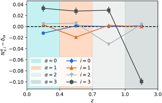
Measurements of |$N_{\gamma ,i}^{\alpha }$| for assigned true redshift interval i. |$N_{\gamma ,i}^{\alpha }$| is the response of the mean shear of galaxy ensemble i, to a shear applied in redshift interval α. In this case our ensembles i correspond to intervals in true redshift. The metacalibration prediction for |$N_{\gamma ,i}^{\alpha }$| in this case is simply the identity matrix: |$N_{\gamma ,i}^{\alpha }=\delta _{i\alpha }$|, since one would expect unity response of galaxies to shear applied in their own redshift interval, and zero response otherwise. Hence we have subtracted δiα in this plot to reduce the dynamic range. The y-axis then demonstrates the biases from assuming the metacalibration-response weighted n(z) as the effective redshift distribution.
The off-diagonal terms in |$N_{\gamma ,i}^\alpha$| are predominantly positive, especially for i = 3, that is for detections assigned to the highest redshift interval. This means that the detections exhibit a positive response to shear applied in the other redshift intervals α ≠ i, a clear detection of the mechanism (ii) described in the previous section, and demonstrated in our simple simulation in Section 1. This effect is potentially important since it implies that there will be extra correlation in the shears measured at different redshifts w.r.t what one would expect from the estimated redshift distribution |$n_{\gamma }^{\text{mcal}}(z)$|. Or put differently, there will be additional tails or broadening in the effective redshift distribution for weak lensing.
5.4 |$N_{\gamma }^{\alpha }$| measurements for photo-z bins
We now repeat the above measurement, but applied to photometric redshift bins, rather than bins of assigned true redshifts. These are the most directly applicable measurements for the DES Y3 weak lensing analyses. We use the same simulations and shear measurements to calculate the integrated effective density |$N_{\gamma ,i}^\alpha$| for photometric redshift bin i. |$N_{\gamma ,i}^\alpha$| is estimated from the simulations in the same way as above but now simply restricting the mean shear calculation to detections assigned to photometric redshift bin i, according to the procedure described in Section 3.7. Note the change in meaning of index i, which now labels the photo-z bin rather than the bin in assigned true redshift.
Fig. 10 shows the difference between the |$N_{\gamma ,i}^\alpha$| measurements and the |$N_{\gamma ,i}^{\alpha ,\text{mcal}}$| predictions for each photo-z bin i. In this case, |$N_{\gamma ,i}^{\alpha ,\text{mcal}}$| is no longer δi,α as before, since for any (i, α) pair, the photo-z bin i includes galaxies outside of the range |$(z_1^\alpha ,z_2^\alpha)$|. Instead, we now calculate |$N_{\gamma ,i}^{\alpha ,\text{mcal}}$| using equation (26), summing over the metacalibration responses for the galaxies in each photo-z bin i. The blue rectangles in Fig. 10 show the resulting |$N_{\gamma ,i}^\alpha - N_{\gamma ,i}^{\alpha ,\text{mcal}}$| values with their estimated uncertainties.
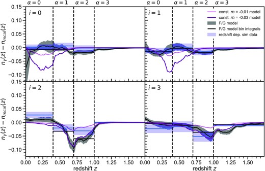
Modelling |$n_{\gamma ,i}^{\text{model}}(z)$| using |$N_{\gamma ,i}^\alpha$| from our image simulations. In each panel, the blue rectangles show |$N_{\gamma ,i}^\alpha -N_{\gamma }^{\alpha ,\text{mcal}}$| for the photometric redshift bin i. The width represents the redshift extent of the interval α and height indicates the 1σ uncertainty on the measurement. The grey band in each panel shows the posteriors of our |$n_{\gamma ,i}^{\text{model}}(z)$| and the horizontal black lines are the integrals over this model which form the predictions for the |$N_{\gamma ,i}^\alpha$| measurements from the simulations. The light and dark purple lines show the models that would result if one used a constant multiplicative bias of −0.01 and −0.03, respectively. It is clear from the simulation data, especially in bin 2, that no constant multiplicative bias model would be sufficient. In particular, at lower redshift in bin 2, they cannot capture the increased response to low redshift shear due to blending.
The measurements are noisier for this case, especially where there is little weight in the underlying n(z), e.g. at high redshift (α = 2 and α = 3) for the first photo-z bin, i = 0. Due to the fact that our photometric redshift pipeline cannot group galaxies perfectly in redshift, the effects from source blending in Fig. 9 are diluted. The model fits that also appear in Fig. 10 are described in the next section.
5.5 nγ(z) bias model constraints for photo-z bins
5.5.1 The model
Due to the limited volume of image simulation data, we can only employ relatively constrained models. For Gi(z), we fit a template with a single free amplitude. The template is built from the flux density of the COSMOS sample in the riz-bands as a function of redshift. This model is motivated by the idea that for random projections, blending effects will be proportional to the flux density of objects.
5.5.2 Fitting procedure
Equipped with simulation measurements of |$N_{\gamma ,i}^\alpha$| and |$\bar{R}_i$|, an estimate of their joint covariance matrix Ci (again estimated by jackknifing over simulated tiles) and a model for nγ(z) with which we can predict them, we can now form a likelihood to constrain that model.
5.6 Model constraints
The posterior constraints on our models are shown in Fig. 10 as the grey bands. We also show the predictions for |$N_{\gamma ,i}^\alpha$| as the horizontal grey lines. We find that our model generally provides a good fit to the data. In this figure, we also show the predictions of a model that employs a constant m per tomographic bin, i.e. |$n_{\gamma ,i}^{\text{model}}(z)= (1+m_i)n_{\gamma ,i}^{\text{mcal}}(z)$|. While this model may be sufficient for the lower redshift tomographic bins, in bin i = 2 we find that it cannot capture the low redshift tails introduced into |$n_{\gamma ,i}^{\text{model}}(z)$|, perhaps due to blending.
These two summary statistics of nγ(z) are probably the two most important for weak lensing analysis, where higher order biases in the redshift distribution are likely to have a subdominant effect to changes in normalization (i.e. multiplicative bias) or mean redshift. The two models give largely similar constraints in m and |$\delta \bar{z}$|, with the fiducial model in general allowing slightly larger shifts in redshift. The first two lines of Table 4 contain these inferred m and |$\delta \bar{z}$| constraints for the two nγ(z) bias models (fiducial and Student’s-t), when applied to the fiducial n(z)s from the image simulations.
Inferred constraints on m and |$\delta \bar{z}$| from the nγ(z) model samples fit to the image simulations measurements. These nγ(z) models are generated by perturbing the image simulation |$n_{\gamma }^{\text{mcal}}(z)$|.
| Quantity | Tomo. bin | Fiducial model | Student’s-t model |
|---|---|---|---|
| m × 100 | 0 | −1.36 ± 0.29 | −1.37 ± 0.29 |
| m × 100 | 1 | −1.78 ± 0.36 | −1.77 ± 0.36 |
| m × 100 | 2 | −2.48 ± 0.41 | −2.52 ± 0.42 |
| m × 100 | 3 | −3.34 ± 0.52 | −3.31 ± 0.52 |
| |$\Delta \bar{z}_0\times 100$| | 0 | −0.65 ± 0.27 | −0.96 ± 0.30 |
| |$\Delta \bar{z}_0\times 100$| | 1 | −0.80 ± 0.31 | −0.76 ± 0.29 |
| |$\Delta \bar{z}_0\times 100$| | 2 | −0.36 ± 0.26 | −0.40 ± 0.19 |
| |$\Delta \bar{z}_0\times 100$| | 3 | −1.13 ± 0.60 | −0.45 ± 0.37 |
The nγ(z) bias model constraints encapsulate our characterization of shear calibration biases for each DES Y3 photometric redshift bin, including redshift dependent effects such as the impact of blending on the effective redshift distribution for lensing. They also include the statistical uncertainty on the calibration due to finite simulation volume. When using the nγ(z) bias model for the real DES Y3 data, we apply it instead to the n(z)s estimated from the DES Y3 data. In the next section, we describe this procedure, and explore potential systematic uncertainties in our corrections, in order to provide statistical and systematic uncertainty priors on the corrections measured from the simulations here.
6 Nγ(Z) CORRECTIONS FOR THE DES Y3 SHEAR CATALOGUE
In Section 5, we generated estimates of the bias in our methodology for constructing the effective redshift distribution for lensing, nγ(z). We did this by comparing direct estimates of nγ(z) from the image simulations, possible only because we know the input shear to the simulations, to the method we use on the Y3 data: the metacalibration response-weighted redshift distribution, |$n_{\gamma }^{\text{mcal}}(z)$|. These bias estimates are intended to be used to make corrections to the redshift distributions used in theory predictions in weak lensing cosmology analyses. In our case, those redshift distributions are those estimated from the DES Y3 data, summarized in Myles et al. (2021), which provide ensembles of redshift distributions constrained by both galaxy flux information, and clustering (Gatti et al. 2020). In Section 6.1, we describe our procedure for applying our corrections to these redshift distributions. This procedure results in a set of nγ(z) samples, which can be sampled over when performing cosmological parameter inference (e.g. using the hyperrank method described in Cordero et al. 2021).
The accuracy of our corrections depends on how realistically we have simulated the DES Y3 data. In Sections 6.2–6.4, we explore this issue by inspecting the sensitivity of our nγ(z) bias corrections to variations in the simulation measurements or simulation analysis choices. Results from these variations feed into our systematic uncertainties.
Finally, in Section 6.5, we summarize our final corrections which include both statistical and systematic uncertainties.
6.1 Applying corrections to the DES Y3 n(z)s
Myles et al. (2021) provide an ensemble of 1000 samples (for each of the four photo-z bins) drawn from the posterior of the set of photo-z bin redshift distributions, constrained by both galaxy flux (including colour) and clustering information. These distributions are already weighted by the metacalibration response estimated from the DES data, so in fact correspond to samples of |$n_{\gamma ,i}^{\text{mcal}}(z)$|. For each of these 1000 samples, we draw 100 randomly chosen samples of our bias model inferred from our simulation measurements, quantified by the functions F(z) and G(z). Then we apply these model biases to |$n_{\gamma ,i}^{\text{mcal}}(z)$| using equation (29) to produce estimates of nγ(z). This process leaves us with 1000 × 100 = 100, 000 nγ(z) samples for each photo-z bin, but note that in practice one could downsample this set of nγ(z)s to a more manageable number depending on the application.
In Fig. 11, we show the distributions of mean multiplicative bias, m (top panels), and mean redshift, |$\bar{z}$| (bottom panels) inferred from these nγ(z) samples. m is calculated as in equation (36) i.e. is simply the normalization of nγ(z) minus 1. In all cases the height of the violin shape is proportional to the fractional weight in the distribution at a given value of the x-axis. The lines labelled ‘fiducial’ represent the inferred m and |$\bar{z}$| distributions for this case. We also list the mean and standard deviation of these m and |$\bar{z}$| distributions in Table 5. We note here that we are in some sense extrapolating the corrections we have inferred from our simulations on to the DES Y3 data, and one must always be careful with extrapolation. However, the fact that the mean m values inferred from the image simulation nγ(z) models (first row of Table 4) are within the 1σ bounds of the ‘fiducial’ Y3 data m priors in Table 5, gives us confidence that this extrapolation is well behaved.
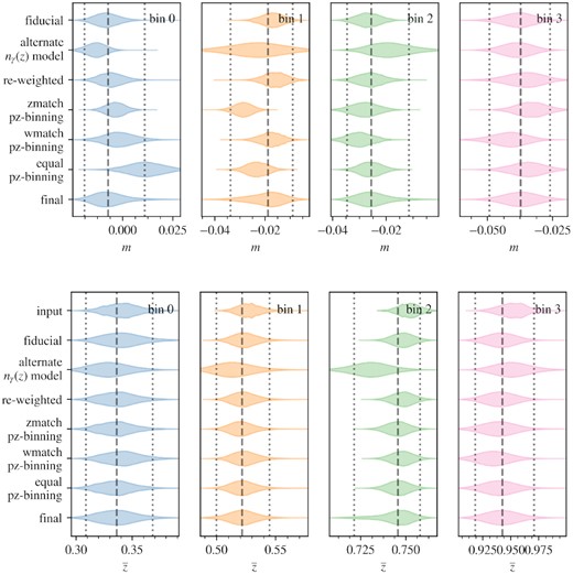
Distributions of the inferred m (top panels) and mean redshift |$\bar{z}$| (bottom panels) of our DES Y3 redshift nγ(z) estimates, generated by applying our simulation corrections to an input ensemble of redshift distributions. For each line nγ(z) corrections are applied from a variation on the fiducial simulation analysis, which have been chosen to expose potential systematic errors in the fiducial approach. The lines marked ‘final’ represent the mixture approach described in Section 6.5, which incorporates systematic uncertainty by mixing together samples from the alternative approaches with the fiducial analysis. In the lower panel, we show also in the first line the distribution of mean redshifts for the input (i.e. before correction) redshift distributions.
Summary statistics of the DES Y3 data nγ(z) distributions, or in the case of the lines labelled ‘input’, input ensemble of redshift distributions i.e. before correction. The ‘input’ lines hence have no associated multiplicative bias m. The column labelled |$\bar{z}$| is the mean and standard deviation of the distribution of mean redshift of nγ(z). The column labelled |$\delta \bar{z}$| is the mean and standard deviation of the distribution of |$\delta \bar{z}$|, which for a given nγ(z), is the difference in mean redshift w.r.t to the mean redshift of the input ensemble of n(z). The column labelled |$\delta \bar{z}_{FG}$| is the mean and standard deviation of the distribution of |$\delta \bar{z}_{FG}$|, which for a given nγ(z), is the difference in mean redshift w.r.t the mean redshift of the specific n(z) sample used to generate the nγ(z).
| Model | Photo-z bin | m × 100 | |$\bar{z}$| | |$\delta \bar{z}\times 100$| | |$\delta \bar{z}_{FG}\times 100$| |
|---|---|---|---|---|---|
| input | 0 | N/A | 0.341 ± 0.016 | 0.000 ± 1.608 | 0.000 ± 0.000 |
| fiducial | 0 | −0.789 ± 0.625 | 0.341 ± 0.019 | −0.021 ± 1.938 | −0.021 ± 0.711 |
| alternate nγ(z) | 0 | −1.346 ± 0.541 | 0.330 ± 0.018 | −1.054 ± 1.834 | −1.054 ± 0.991 |
| re-weighted | 0 | −0.574 ± 0.615 | 0.337 ± 0.017 | −0.406 ± 1.750 | −0.406 ± 0.353 |
| zmatch pz | 0 | −0.368 ± 0.481 | 0.335 ± 0.016 | −0.565 ± 1.644 | −0.565 ± 0.143 |
| wmatch pz | 0 | −0.172 ± 0.790 | 0.341 ± 0.018 | −0.009 ± 1.766 | −0.009 ± 0.361 |
| equal pz | 0 | 1.117 ± 0.908 | 0.335 ± 0.017 | −0.580 ± 1.651 | −0.580 ± 0.212 |
| final | 0 | −0.627 ± 0.908 | 0.336 ± 0.018 | −0.467 ± 1.846 | −0.467 ± 0.758 |
| input | 1 | N/A | 0.528 ± 0.013 | −0.000 ± 1.280 | 0.000 ± 0.000 |
| fiducial | 1 | −1.703 ± 0.446 | 0.524 ± 0.013 | −0.367 ± 1.344 | −0.367 ± 0.215 |
| alternate nγ(z) | 1 | −2.315 ± 1.080 | 0.515 ± 0.018 | −1.267 ± 1.812 | −1.267 ± 1.441 |
| re-weighted | 1 | −1.589 ± 0.461 | 0.523 ± 0.013 | −0.467 ± 1.341 | −0.467 ± 0.193 |
| zmatch pz | 1 | −2.869 ± 0.375 | 0.521 ± 0.012 | −0.725 ± 1.212 | −0.725 ± 0.358 |
| wmatch pz | 1 | −1.763 ± 0.452 | 0.524 ± 0.013 | −0.385 ± 1.335 | −0.385 ± 0.218 |
| equal pz | 1 | −2.308 ± 0.435 | 0.522 ± 0.013 | −0.561 ± 1.311 | −0.561 ± 0.282 |
| final | 1 | −1.984 ± 0.779 | 0.521 ± 0.015 | −0.671 ± 1.506 | −0.671 ± 0.833 |
| input | 2 | N/A | 0.750 ± 0.006 | −0.000 ± 0.629 | 0.000 ± 0.000 |
| fiducial | 2 | −2.667 ± 0.458 | 0.746 ± 0.006 | −0.365 ± 0.632 | −0.365 ± 0.209 |
| alternate nγ(z) | 2 | −1.649 ± 0.892 | 0.729 ± 0.012 | −2.048 ± 1.173 | −2.048 ± 1.251 |
| re-weighted | 2 | −2.570 ± 0.494 | 0.746 ± 0.006 | −0.355 ± 0.641 | −0.355 ± 0.152 |
| zmatch pz | 2 | −2.759 ± 0.511 | 0.743 ± 0.006 | −0.676 ± 0.637 | −0.676 ± 0.204 |
| wmatch pz | 2 | −2.967 ± 0.483 | 0.745 ± 0.006 | −0.411 ± 0.627 | −0.411 ± 0.202 |
| equal pz | 2 | −2.558 ± 0.430 | 0.743 ± 0.006 | −0.613 ± 0.626 | −0.613 ± 0.256 |
| final | 2 | −2.412 ± 0.760 | 0.741 ± 0.011 | −0.830 ± 1.071 | −0.830 ± 0.959 |
| input | 3 | N/A | 0.946 ± 0.015 | 0.000 ± 1.524 | 0.000 ± 0.000 |
| fiducial | 3 | −3.794 ± 0.718 | 0.934 ± 0.013 | −1.170 ± 1.317 | −1.170 ± 1.046 |
| alternate nγ(z) | 3 | −3.780 ± 0.606 | 0.945 ± 0.019 | −0.060 ± 1.913 | −0.060 ± 0.977 |
| re-weighted | 3 | −3.574 ± 0.841 | 0.933 ± 0.014 | −1.304 ± 1.378 | −1.304 ± 1.333 |
| zmatch pz | 3 | −3.253 ± 0.589 | 0.933 ± 0.017 | −1.313 ± 1.698 | −1.313 ± 0.902 |
| wmatch pz | 3 | −4.179 ± 0.852 | 0.927 ± 0.015 | −1.875 ± 1.490 | −1.875 ± 1.575 |
| equal pz | 3 | −3.442 ± 0.690 | 0.933 ± 0.015 | −1.277 ± 1.548 | −1.277 ± 1.037 |
| final | 3 | −3.692 ± 0.761 | 0.936 ± 0.017 | −1.008 ± 1.672 | −1.008 ± 1.290 |
In the next three sub-sections, we test for sensitivity of the inferred m and |$\delta \bar{z}$| priors to various potential systematics in our simulation corrections.
6.2 Alternative photo-z-binning schemes
Given the range of viable different photo-z binning schemes presented in Section 3.7, we test for the sensitivity of our corrections to this choice, and include a corresponding contribution to our systematic uncertainties related to this choice. For each of the photo-z binning schemes, we repeat the inference of nγ(z) corrections performed in Section 5.5, but now using the slightly different |$N_{\gamma ,i}^\alpha$| and |$\bar{R}_i$| measurements resulting from changing the photo-z binning scheme. This results in sets of F(z) and G(z) samples for each photo-z binning scheme, from which we can generate nγ(z) samples for the DES Y3 data, following the procedure in Section 6.1. The inferred ms and |$\bar{z}$|s for these cases are also shown in Fig. 11, as the lines labelled ‘zmatch pz-binning’, ‘wmatch pz-binning ’, and ‘equal pz-binning’ (see Section 3.7 for the details of the binning methods).
6.3 Simulation re-weighting
The overall agreement between object properties and density in the simulation and real data is very good, both globally and within each redshift bin. To validate that any remaining differences would not significantly modify our inferred shear calibration, we focus on several properties most likely to correlate with the amount of blending, which is our main source of shear calibration bias.
We implement a re-weighting scheme designed to match the small-scale counts of close pairs in the DES Y3 data, including the magnitude dependence of this behaviour. We believe this should provide a first order estimate of the potential impact of ignoring galaxy clustering in our simulations, which although weak for our wide-in-redshift photometric redshift bins, may have non-negligible impact on the amount of blending.
We choose three quantities on which to re-weight: the magnitude (calculated from the mean of the flux in the r, i, and z bands), the distance to the nearest neighbour, and the magnitude of the nearest neighbour (again based on the r, i, and z bands). The neighbour can be any detected object with non-negative flux (i.e. we do not restrict the neighbour candidates to objects passing shape catalogue cuts). We then aim to produce a set of weights to apply to the simulation results that will improve the match of the joint distributions of these quantities between simulations and data.
To accomplish this, we use k-means clustering to define clusters of these three quantities based on 200 000 randomly selected objects in each photo-z bin. We then assign all objects in both the simulations and DES Y3 data to these clusters. Weights are produced for each photo-z bin by taking the ratio of the number of objects assigned to each data cluster to the number assigned to each simulation cluster. We show in Fig. 12 that this re-weighting of objects improves agreement with the data.
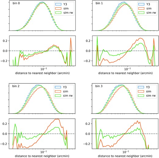
Distribution of distance to nearest neighbour for each photo-z bin. The first and third rows show these distributions (as normalized histograms) for the Y3 data (‘Y3’, blue), the image simulations (‘sim’, orange), and the re-weighed simulations (‘sim rw’, green – using the re-weighting procedure described in Section 6.3). The second and fourth rows show the fractional difference of the ‘sim’ and ‘sim rw’ distributions with respect to the Y3 data distributions. In all cases, the agreement between simulations and data is improved by the re-weighting procedure.
We update the weights of our simulated shear catalogues, and re-derive the nγ(z) correction model (by re-performing the |$N_{\gamma ,i}^\alpha$| and |$\bar{R}_i$| measurements and the |$n_{\gamma ,i}^{\text{model}}(z)$| fits). We again apply the resulting F(z) and G(z) corrections to the Y3 data n(z) ensemble to get an ensemble of nγ(z) samples. The inferred ms and |$\bar{z}$|s for these cases are also shown in Fig. 11, as the lines labelled ‘re-weighted’. The impact on |$\bar{z}$| is small, with at most 0.2 per cent shifts in the mean. There is also a small (between 0.1 and 0.2 per cent), coherent shift in the mean of the m distributions to less negative values for all photo-z bins. While small, we find the sign surprising, since we expect this re-weighting procedure to increase the number of close pairs in the simulation, and thus increase the impact of blending on the multiplicative bias.
We note that this re-weighting procedure will not include all the potentially relevant effects present in a galaxy sample with realistic clustering. We discuss in detail in Section 7 the possibility that we have underestimated blending-related biases as a result of this.
6.4 Alternative nγ(z) bias parametrization
We chose a fiducial functional form for the multiplicative correction F(z) in our nγ(z) bias model. This was based on the perturbative expansion in equation (31), applied to the n(z) model in equation (32). Note that we only use this simple parametric model to generate a functional form for the perturbations from |$n_{\gamma }^{\text{mcal}}(z)$|; we do not use the parametric fit directly. We have also investigated the use of a Student’s-t model, which we use to generate an alternative set of F(z) and G(z) samples with which we correct the DES Y3 n(z) ensemble. The resulting inferred m and |$\delta \bar{z}$| distributions are shown in Fig. 11, as the lines labelled ‘alternate nγ(z) model’. We observe some non-negligible shifts with respect to the fiducial m and |$\bar{z}$|. The largest are for photo-z bin 2, with a shift in the mean of the m distribution of |$1.0{{\ \rm per\ cent}}$|, and a shift in the mean |$\bar{z}$| of |$-1.7{{\ \rm per\ cent}}$|. We also see broadening of the |$\bar{z}$| distributions for all photo-z bins.
6.5 Final nγ(z) priors
We can generate the final prior on nγ(z) simply by combining the samples from the individual cases in the correct proportions. The inferred m and |$\bar{z}$| distributions for this final prior is shown in the bottom rows of Fig. 11. The grey dotted vertical lines show the 5th and 95th percentiles of this final prior, while the dashed vertical line shows its median.
One can see qualitatively by eye that this mixture prior accounts for systematic uncertainties with a longer tail where there is an outlier in one of the variations. For example, the m distribution for bin 0, while still centred close to the fiducial case, gains extra weight in the tail to high m due to the outlying m distribution for the ‘equal’ photo-z binning variation. Similarly, the significant shift for the alternate nγ(z) variation in the |$\bar{z}$| distribution for bin 2 is accounted for by a large tail to low |$\bar{z}$| values.
We note that the m and |$\delta \bar{z}$| statistics presented here are summary statistics of the full corrections, which are incorporated into perturbed nγ(z) samples. It is these nγ(z) samples that should be used in theoretical predictions of weak lensing statistics (e.g. shear correlation functions or tangential shear) for the DES Year 3 shear catalogue. An algorithm for efficiently sampling over discrete nγ(z) samples, such as that presented in Cordero et al. (2021) can be used (or alternatively one could directly sample the likelihood in equation 35, simultaneously with the likelihood for the Year 3 weak lensing statistics). However, for some applications, it may be desirable and sufficiently accurate to directly use the inferred m and |$\delta \bar{z}$| statistics as approximate corrections to the effective redshift distribution, and sample over them as nuisance parameters. The accuracy of such an approach should be validated against the use of the full corrections.
7 DISCUSSION
Image simulations have long been recognized as an essential tool for calibrating shear estimation pipelines, and have played a role in providing the shear calibration for all recent weak lensing cosmology analyses. While current methodologies like metacalibration have made major strides in dealing with well-studied shear estimation biases like noise bias and model bias, we are now entering an era of weak lensing data that is both deep, resulting in significant blending of galaxy surface brightness profiles, and voluminous, thus statistically powerful enough to have very strict accuracy requirements.
In this work, we present realistic image simulations designed to accurately calibrate many of the complexities in analysing real imaging data. By using a combination of morphological information from HST and flux information from DES Deep Fields, we make use of an input galaxy sample with realistic joint distributions of flux (in multiple bands) and morphology. This, along with careful simulation of the observational characteristics of real DES Y3 data, gives us confidence that measurements of biases can be reliably applied as calibration corrections. This multiband weak lensing calibration simulation allows us to perform the same photometric redshift inference as is performed on the real data, allowing reliable and consistent corrections for each photometric redshift bin.
While we believe these simulations are sufficiently realistic given the requirements of the DES Year 3 cosmology analyses, they do of course involve approximations and shortcuts that may not be sufficiently accurate for future analyses. We do not simulate the estimation of the WCS solution, PSF, background levels or noise levels in our simulations, under the assumption that any errors in our estimation of these in the real data are negligible. These assumptions should be carefully re-examined for more precise upcoming weak lensing data sets.
In addition, we simulated galaxies with random sky positions, rather than a realistic level of clustering. While our re-weighting procedure in Section 6.3 can increase the number of pairs of close detected objects, it does not explicitly match the number of groups of more than two close detected objects, however, at current number densities, we expect those to be much less frequent. The re-weighting also cannot impact the statistics of undetected objects, and so will not change the frequency of detected galaxies having close, undetected neighbours. This specific case is investigated in detail by Euclid Collaboration (2019), who demonstrate that for Euclid-like data, the clustering of faint galaxies around the bright ones used for shape measurement can induce a multiplicative bias of |$\sim -0.5{{\ \rm per\ cent}}$| (with respect to the case where the faint galaxies are unclustered). Since this is of the same order as our statistical uncertainties, it is worth careful consideration.
We first note that the only conclusive way to judge the impact of the clustering of undetected galaxies is to simulate it. However, generating a weak lensing calibration image simulation with realistic clustering statistics, as well as the realistic distributions of measured properties demonstrated here (Section 3.6) is an ongoing challenge. Current cosmological simulations which include the former have not been demonstrated to produce the high level of agreement with real data at the image level that is required for weak lensing calibration. In the absence of such a simulation, we make some arguments that the size of the biases estimated by Euclid Collaboration (2019) are likely an upper limit on the size of biases likely to be generated by clustering of undetected objects in DES Year 3.
First, the DES Year 3 data are shallower than the Euclid-like simulations in Euclid Collaboration (2019), hence in general blending-related biases are lessened. Secondly, the ‘faint’ galaxies in Euclid Collaboration (2019) are defined as having S/N < 10. We include all objects detected by SExtractor (and with positive flux) in our re-weighting procedure, which therefore only misses out on the S/N < <10 objects that are undetected by SExtractor. Thirdly, we are using metacalibration, which has some robustness to blending – for very close pairs which are always detected as a single object, metacalibration performs extremely well (as demonstrated in Sheldon et al. 2020), because it calibrates the response of the measurement to shear of all the light in the system. This is not the case for the shape measurement methods used in Euclid Collaboration (2019), which we would expect to be more sensitive to ‘model bias’ arising from the unusual apparent morphology of blended systems. Similarly, metacalibration’s insensitivity to noise bias means faint objects that are always undetected are unlikely to cause significant biases; their contribution behaves largely as extra noise.
While these arguments are somewhat based on intuition rather than extensive simulation results, given constraints on time and computing resources, we think they justify our approach and priorities for the calibration of this intermediate data set. None the less, we recommended that Amon et al. (2021) include a robustness test where an additional multiplicative bias with prior width |$1{{\ \rm per\ cent}}$| was marginalized over in the cosmological inference from cosmic shear. This extra bias was assumed to be coherent across redshift bins, and represents a pessimistic interpretation of the potential bias arising from the effect explored by Euclid Collaboration (2019). They find negligible change in the constraint on S8 = σ8(Ωm/0.3)0.5, likely due to the dominance of other sources of systematic uncertainty.
Another potential limitation of our simulations is the limited size of our input galaxy catalogue (see e.g. Kannawadi, Mandelbaum & Lackner 2015 for an investigation of the impact of limited input catalogue size in weak lensing image simulations), which came from the COSMOS region, motivated by the availability of HST imaging that provides precise morphological information for our input galaxies. While our detailed comparisons of the simulation outputs and the real DES Year 3 data suggest that cosmic variance in the input catalogue is not a huge effect (and this conclusion agrees with that of Kannawadi et al. 2019), we would recommend investigations of the possibility of larger reliable input catalogues from deep ground-based imaging only (as measured by Hartley et al. 2020 and used in injection simulations by Everett et al. 2020). The planned LSST deep-drilling fields would be a valuable source of such data.
Conceptually, we have stressed the importance of characterizing biases due to blending via their impact on the effective redshift distribution. When blending becomes an important contributor to shear calibration biases, photo-z and shear inference can no longer be cleanly decoupled. Folding both photo-z and shear calibration biases into an effective redshift distribution for lensing, nγ(z), is both a compact approach, and very general in that nγ(z) is the key observational quantity required to make theoretical predictions for most weak lensing signals of interest. The normalization of nγ(z) corresponds to the traditional mean multiplicative bias, 1 + m.
Via simulations with redshift-dependent shear signals, we have provided a methodology for directly estimating nγ(z) integrated over finite redshift intervals. The key point in this approach is that the value of the effective redshift distribution at a given redshift is defined by the response of the ensemble to shear at that redshift. Therefore, only by simulating such a shear signal can the effective redshift distribution be estimated robustly. We believe that with the increased depth (and therefore increased blending) and stricter accuracy requirements of future surveys such as the Rubin Observatory and Euclid, such an approach will become essential i.e. nγ(z) is the quantity that must be accurately characterized for reliable cosmological inference, which is a requirement beyond the traditional approach of characterizing the multiplicative bias m.
In Section 6, we propagated our simulation measurements through to corrections for the DES Y3 redshift distributions, producing from an input ensemble of redshift distributions, an output ensemble of effective redshift distributions, nγ(z) ready for use in the Year 3 weak lensing cosmology analyses. This output ensemble includes both statistical (due to finite simulation volume) and systematic (due to potential simulation inaccuracies) uncertainties. These nγ(z) should be used directly in the theoretical predictions for weak lensing statistics like the shear correlation functions and galaxy–galaxy lensing tangential shear, as the effective redshift distribution entering the lensing kernel. Note that the (in general non-unity) normalization of the effective redshift distributions should be retained in the calculations, or applied to the resulting theory prediction if using a numerical code that normalizes the redshift distribution internally. This data will be made available along with the DES Year 3 shear catalogues, on publication of the key Year 3 cosmology analyses, as part of the DES Y3 coordinated release.11
SUPPORTING INFORMATION
Appendix A: Shear and redshift bias parameters used prior to unblinding the analysis
Appendix B: Simulation validation tests
Appendix C: PIFF PSF model smoothing for simulations
Please note: Oxford University Press is not responsible for the content or functionality of any supporting materials supplied by the authors. Any queries (other than missing material) should be directed to the corresponding author for the article.
ACKNOWLEDGEMENTS
This paper has gone through internal review by the DES collaboration. We thank the internal reviewers for their very helpful suggestions for improving the paper.
Funding for the DES Projects has been provided by the U.S. Department of Energy, the U.S. National Science Foundation, the Ministry of Science and Education of Spain, the Science and Technology Facilities Council of the United Kingdom, the Higher Education Funding Council for England, the National Center for Supercomputing Applications at the University of Illinois at Urbana-Champaign, the Kavli Institute of Cosmological Physics at the University of Chicago, the Center for Cosmology and Astro-Particle Physics at the Ohio State University, the Mitchell Institute for Fundamental Physics and Astronomy at Texas A&M University, Financiadora de Estudos e Projetos, Fundação Carlos Chagas Filho de Amparo à Pesquisa do Estado do Rio de Janeiro, Conselho Nacional de Desenvolvimento Científico e Tecnológico and the Ministério da Ciência, Tecnologia e Inovação, the Deutsche Forschungsgemeinschaft and the Collaborating Institutions in the Dark Energy Survey.
The Collaborating Institutions are Argonne National Laboratory, the University of California at Santa Cruz, the University of Cambridge, Centro de Investigaciones Energéticas, Medioambientales y Tecnológicas-Madrid, the University of Chicago, University College London, the DES-Brazil Consortium, the University of Edinburgh, the Eidgenössische Technische Hochschule (ETH) Zürich, Fermi National Accelerator Laboratory, the University of Illinois at Urbana-Champaign, the Institut de Ciències de l’Espai (IEEC/CSIC), the Institut de Física d’Altes Energies, Lawrence Berkeley National Laboratory, the Ludwig-Maximilians Universität München and the associated Excellence Cluster Universe, the University of Michigan, NFS’s NOIRLab, the University of Nottingham, The Ohio State University, the University of Pennsylvania, the University of Portsmouth, SLAC National Accelerator Laboratory, Stanford University, the University of Sussex, Texas A&M University, and the OzDES Membership Consortium.
Based in part on observations at Cerro Tololo Inter-American Observatory at NSF’s NOIRLab (NOIRLab Prop. ID 2012B-0001; PI: J. Frieman), which is managed by the Association of Universities for Research in Astronomy (AURA) under a cooperative agreement with the National Science Foundation.
The DES data management system is supported by the National Science Foundation under Grant Numbers AST-1138766 and AST-1536171. The DES participants from Spanish institutions are partially supported by MICINN under grants ESP2017-89838, PGC2018-094773, PGC2018-102021, SEV-2016-0588, SEV-2016-0597, and MDM-2015-0509, some of which include ERDF funds from the European Union. IFAE is partially funded by the CERCA program of the Generalitat de Catalunya. Research leading to these results has received funding from the European Research Council under the European Union’s Seventh Framework Program (FP7/2007-2013) including ERC grant agreements 240672, 291329, and 306478. We acknowledge support from the Brazilian Instituto Nacional de Ciência e Tecnologia (INCT) do e-Universo (CNPq grant 465376/2014-2).
This manuscript has been authored by Fermi Research Alliance, LLC under Contract No. DE-AC02-07CH11359 with the U.S. Department of Energy, Office of Science, Office of High Energy Physics.
NM acknowledges support from a European Research Council (ERC) Starting Grant under the European Union’s Horizon 2020 research and innovation programme (grant agreement no. 851274). MRB is supported by DOE grant DE-AC02-06CH11357. This work was supported by the Department of Energy, Laboratory Directed Research and Development program at SLAC National Accelerator Laboratory, under contract DE-AC02-76SF00515 and as part of the Panofsky Fellowship awarded to DG. MJ is partially supported by the U.S. Department of Energy grant DE-SC0007901 and funds from the University of Pennsylvania. AC acknowledges support from NASA grant 15-WFIRST15-0008. RR, IH, and SB acknowledge support from the European Research Council in the form of a Consolidator Grant with number 681431. IH also acknowledges support from the Beecroft Trust.
We gratefully acknowledge the computing resources provided on Bebop, a high-performance computing cluster operated by the Laboratory Computing Resource Center at Argonne National Laboratory, and the RHIC Atlas Computing Facility, operated by Brookhaven National Laboratory.
This research used resources of the National Energy Research Scientific Computing Center (NERSC), a U.S. Department of Energy Office of Science User Facility operated under Contract No. DE-AC02-05CH11231.
DATA AVAILABILITY
All DES Year 3 cosmology catalogues, including calibrations, will be made available at https://www.darkenergysurvey.org/the-des-project/data-access/ on publication of the key cosmological results.
Footnotes
see SExtractor documentation at http://mensa.ast.uct.ac.za/~holwerda/SE/Manual.html or https://www.astromatic.net/pubsvn/software/sextractor/trunk/doc/sextractor.pdf for more details on these quantities.
