Measurement of the anisotropy power spectrum of the radio synchrotron background Free

ABSTRACT

1 INTRODUCTION

Figure 1.

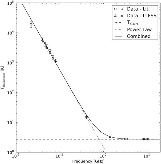
The measured radio background brightness spectrum in radiometric temperature units reproduced from Dowell & Taylor (2018), as measured by the few measurements and maps where an absolute zero-level calibration was either explicit or obtained, including that work. The brightness shows a clear power-law rise at frequencies below ∼10 GHz, above the otherwise dominant CMB level represented by the dashed line.

Open in new tabDownload slide

The reported bright background level is now in extreme tension with estimates of its expected level from the known radio emission mechanisms in the Universe, as recently summarized in Singal et al. (2018). Several works have considered deep radio source counts and limited the integrated surface brightness from known classes of extragalactic radio sources to only around one-fifth of the radio background brightness level (e.g. Condon et al. 2012; Vernstrom et al. 2014), including recently at 144 MHz (Hardcastle et al. 2020). Thus, to achieve the measured radio background level from point sources would require an entirely new, incredibly numerous, heretofore unobserved population of low-flux radio sources. As an alternative, various types of diffuse extragalactic sources such as cluster mergers (e.g. Fang & Linden 2016) and intergalactic dark matter decays and annihilations in galaxies, clusters, and filaments (e.g. Fornengo et al. 2011; Hooper et al. 2012) have been proposed. Alternatively, a large, bright, roughly spherical synchrotron halo surrounding our Galaxy could explain part of the background (e.g. Subrahmanyan & Cowsik 2013). However, such a large, bright halo would make our Galaxy unique among nearby spiral galaxies (Singal et al. 2015) and would overturn our current understanding of the high-latitude Galactic magnetic field (Singal et al. 2010).

One realm in which the RSB is almost completely unexplored is in its anisotropy. Studies of temperature anisotropy power spectra have helped confirm the source populations responsible for the cosmic infrared (e.g. Ade et al. 2011; George et al. 2015) and gamma-ray (e.g. Broderick et al. 2014) backgrounds, and have been the most important component of CMB science thus far (e.g. Bennett et al. 2013).

The only direct constraints available in the literature on the anisotropy of the RSB at the most relevant angular scales are from confusion noise limits at a few discrete scales and based on measurements where considerations of the radio background in particular were incidental. These include decades-old measurements in the GHz range overwhelmed by the CMB by an order of magnitude or greater, specifically based on observations made with the Very Large Array at 8.4 GHz (Partridge et al. 1997) and 4.9 GHz (Fomalont et al. 1988), and the Australia Compact Telescope Array at 8.7 GHz (Subrahmanyan et al. 2000). There are also recent measurements of the sky power spectrum at 150 MHz in several fields made with the Giant Metrewave Radio Telescope recently presented in Choudhuri et al. (2020). The results presented there are in a more limited angular scale range, and in fields with higher Galactic diffuse emission structure contribution, than those presented here, and did not directly address specifically the question of the anisotropy power of the RSB. At larger angular scales than those considered here, where the angular power is dominated by the large-scale Galactic diffuse synchrotron structure, there are determinations of the angular power at 408 MHz reported by La Porta et al. (2018).

In this work, we present a power spectrum of measured anisotropies of the RSB over the angular range from 2° to 0.2 arcmin based on dedicated LOw-Frequency ARray (LOFAR; van Haarlem et al. 2013) observations at 140 MHz of two 18-deg² fields. Section 2 describes the observations and data reduction and analysis methods, Section 3 presents the resulting power spectra, Section 4 explores possible point source populations that could produce the measured anisotropy power, and Section 5 presents a discussion. Appendix  A provides a reference for considering the conversion factors between different computations and scalings of angular power that are relevant when bridging regimes and methods of determination where different conventions are in use.

2 OBSERVATIONS AND DATA REDUCTION

We use data from 8 h of dedicated observing with LOFAR in high-band antenna dual mode with Dutch stations only (23 core, 14 remote) in the band from 110 to 190 MHz on 2019 November 27. As optimally this measurement should be done on a region with the minimum amount of Galactic diffuse foreground spatial structure, we chose a field centred on the Galactic Northern hemisphere ‘coldest patch’ (Kogut et al. 2011; |$9^{\rm h}\, 38^{\rm m}\, 41^{\rm s}$| +30°49′12″, |$l=196{_{.}^{\circ}}0\, b =48{_{.}^{\circ}}0$|⁠), the region of lowest measured diffuse emission absolute temperature and thus where the integrated line-of-sight contribution through the Galactic components is minimal. LOFAR allows a simultaneous observation of an additional field offset by 15° in an adjacent 48-MHz wide band, so we chose a location towards the North Galactic Pole from the coldest patch of |$10^{\rm h}\, 25^{\rm m}\, 00^{\rm s}$| +30°00′00″ (l=199|${_{.}^{\circ}}$|0|$\, b$|=57|${_{.}^{\circ}}$|9), which should have a slightly higher but still nearly minimal total Galactic contribution. Fig. 2 shows a schematic representation of the observed fields relative to a commonly employed simple model of the Galactic diffuse radio emission structure. The data cube consists of 666 baselines (all pairs of correlations) with four linear polarization pairs per visibility in 243 frequency channels with 2-s integrations for a total of 1.4 TB of data per target field. The 243 frequency channels are of equal width of 180 KHz, and the filtering is done with a polyphase filter bank. In addition to the target fields, we observed the flux calibrator 3C 295.

Figure 2.

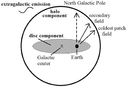
Schematic representation of the coldest patch and secondary target fields observed in this work in the context of a simple model of Galactic diffuse radio emission consisting of an ellipsoidal plane-parallel component due to the Galactic disc and a larger, spherical halo component, each centred on the Galactic Centre. The coldest patch target field is in the direction of minimal integrated line-of-sight total contribution from the two components in the Galactic Northern hemisphere. Such two-component models of large-scale diffuse Galactic radio emission are commonly utilized (e.g. Subrahmanyan & Cowsik 2013; Singal et al. 2015).

Open in new tabDownload slide

Because we are interested in scales that are much larger than the effect of ionospheric activity, we only perform direction-independent calibration, thereby avoiding the effect of signal suppression that might incur during direction-dependent calibration. We have used two different methods for direction-independent calibration and imaging. The first approach is to use prefactor,¹ the standard automated LOFAR direction-independent calibration pipeline (van Weeren et al. 2016; Williams et al. 2016), which makes use of several software packages, including the Default Pre-Processing Pipeline (dp3; van Diepen, Dijkema & Offringa 2018), LOFAR SolutionTool (losoto; de Gasperin et al. 2019), and aoflagger (Offringa, van de Gronde & Roerdink 2012). Because this pipeline has not been developed for power spectrum experiments, for verification we also calibrate our data in a manual approach.

Manual calibration is only performed for the coldest patch field. For manual calibration, we start with running aoflagger to flag outlying data points due to radio-frequency interference (RFI) contamination and one outlying station. We perform initial flux and phase calibrations for each sub-band using the flux calibrator observation, which are then applied to the target fields. We image the target fields with wsclean (Offringa et al. 2014) with primary beam correction and standard clean settings to extract an initial point source model for self-calibration. Specifically, we first run the source extractor aegean (Hancock, Trott & Hurley-Walker 2018) with a high flux threshold of 9σ to extract a shallow model, containing about 300 sources. Following this, we run self-calibration using the model on 25 sub-bands and image at a higher resolution of 45 arcsec. We next re-run aegean with a lower flux threshold (7σ), extracting 2396 sources.

Many of these sources are near the edge of the primary beam and so are likely false detections. We cut out all sources that are at a place in the image where the beam has less than 5 per cent gain, reducing the model to 644 sources with almost no false positives. Extended sources, including one prominent Fanaroff–Riley type II (FR II) galaxy, are excluded from calibration. Source 4C 32.30 with flux 3.6 Jy (Waldram et al. 1996) is near the middle of the coldest patch target field and is used for flux calibration. Using these full calibration solutions, we re-image the target field with wsclean with 20-arcsec resolution. An image of the coldest patch target field is shown in Fig. 3.

Figure 3.

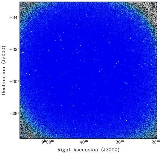
An image of the coldest patch target field resulting from the imaging procedure discussed in Section 2. The synthesized beam measures 1.5 arcmin× 1 arcmin. This field contains 3.6-Jy source 4C 32.30, which can be used for self-flux calibration, and an extended FR II galaxy (visible just to the lower right-hand side of the middle of the field). All sources are removed for power spectrum determination, as point sources manifest power on all angular scales.

Open in new tabDownload slide

The results of the automated and manual approach are found to be similar on the coldest patch field, so we process the secondary target field only with the automated approach using prefactor. Before making power spectra, we subtract the foreground sources using a deep wsclean multifrequency deconvolution using automasking (Offringa & Smirnov 2017). The automasking ensures that all sources ≥7σ are subtracted to a 1σ level. To avoid subtracting a diffuse component, we do not use multiscale clean.

3 POWER SPECTRUM

3.1 Full angular power spectrum

Our angular power spectrum pipeline is based on the pipeline described by Offringa, Mertens & Koopmans (2019), which is originally written for the LOFAR Epoch of Reionization project (Mertens et al. 2020). Our angular pipeline produces a power spectrum of fluctuations from the source-removed target field images. We use the central 4.3 deg² of each target field image for the determination of the angular power spectra. A quantitative discussion of the procedure for forming a power spectrum from an interferometric image is presented in Appendix  A. The steps in making a power spectrum are as follows.

• Make naturally weighted images using multifrequency synthesis from the source-subtracted data. We use wsclean for this with increased accuracy settings (see Offringa et al. 2019).

• Convert the images of flux density into units of temperature (kelvin) using equation (A17).

• Take the spatial Fourier transform of the images and point spread functions (PSFs) to create a grid in complex (u, v) space for both.

• Elementwise divide the complex uv images by the complex value of the uv PSFs.

• Average the power in annuli and normalize these.

This method of determining the power spectrum, where we correct for the (in our case, natural) image weighting function in uv space, alleviates the need to perform a bias correction of the power spectrum. Otherwise, image-based reconstruction of power spectra can give a biased estimate of the true sky signal due to the correlated noise in the image domain (Dutta & Nandakumar 2019).

The resulting power spectrum of fluctuations is shown in Fig. 4, for both the coldest patch and secondary target fields. We also show the spectrum of fluctuations calculated for twelve 4-MHz wide sub-bands separately. The lowest frequency sub-band has approximately 17 times more power in these K² units than the highest frequency sub-band because of the spectral dependence of synchrotron radiation (cf. equation 1), which is a bit over four times as bright in radiometric temperature units (and thus around 17 times as bright in K² units) at 190 GHz than at 110 GHz. The angular power is lower in the full bandwidth because of more complete uv coverage.

Figure 4.

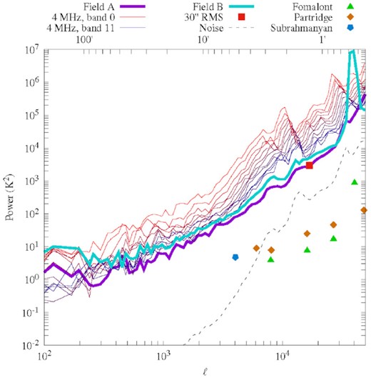
Measured anisotropy power spectrum of the radio sky centred at 140 MHz. Shown are curves for the full bandwidth of the coldest patch field (field A) and the secondary field (field B), as well as for twelve 4-MHz wide sub-bands of field A. The anisotropy in field A deduced by considering the average noise per beam in the image with the synthesized beam tapered to 30-arcsec FWHM is also shown and agrees at the relevant angular scale, given by equation (4). We also show comparison levels inferred by the noise per beam at 8.7, 8.4, and 4.9 GHz in different fields as calculated by Holder (2014) and scaled here to 140 MHz assuming a synchrotron power law of −2.6 in radiometric temperature units. The amount of angular power is ∼1.4 times higher for field B compared to field A (in K² units) across a range of angular scales, as discussed in Section 5. All angular powers are expressed here in the |$\left({\Delta T} \right)_\ell ^2$| normalization.

Open in new tabDownload slide

These measurements will have a contribution from the noise of the instrument. To calculate this contribution, we extract Stokes V visibilities and measure the differential variance between consecutive Stokes V visibilities in time, multiply by 2, and assume that this is a representative noise value for all visibilities. We calculate the noise power spectrum by replacing all visibilities by randomly sampled Gaussian values with the calculated variance, produce images, and calculate a power spectrum from the images as described. The result is shown as the dashed line in Fig. 4. Given that the noise power is at least an order of magnitude below the measured power, clearly our measured power is dominated by something other than the system noise. Additionally, while one would expect the power in the full band to be the average of the sub-bands for the case of noise-dominated power, in this case with the noise contribution sub-dominant, the more complete uv coverage of the full band will result in lower angular power.

3.2 Power from rms fluctuations

We can also calculate the power on a specific, discrete angular scale in a completely different, complementary way, following a procedure discussed in Holder (2014).

• The noise per beam in the image ΔS_Jy/PSF is measured with the synthesized beam tapered to 30-arcsec full width at half-maximum (FWHM). The noise level of this image is 720 |$\mu$|Jy.

• The beam is fitted to an elliptical Gaussian with major and minor axes w_maj and w_min to calculate the synthesized beam solid angle in radians,

  $$\begin{eqnarray*} \Omega _\textrm {PSF}=\pi (w_{\rm maj} \times w_{\rm min}) \times \left(\frac{1}{60} \right)^2 \times \left(\frac{\pi }{180}\right) \times \left(\frac{1}{4 \log 2}\right). \end{eqnarray*}$$

  (2)
• The resulting temperature fluctuation ΔT is calculated by

  $$\begin{eqnarray*} \Delta T = \Delta S_\textrm {Jy/PSF} \frac{ 10^{-26} c^2 }{ 2 k_{\rm B} \nu ^2 \Omega _\textrm {PSF}}, \end{eqnarray*}$$

  (3)

  to achieve ΔT on the angular scale corresponding to a Gaussian beam of 30-arcsec FWHM.

3.3 Power from potentially unremoved point sources

In order to quantify the contribution of potentially unremoved point sources in the images to the measured angular power, we created a Monte Carlo catalogue of simulated sources. We interpolate the simulated sources on to a grid (using sinc interpolation) and simulate visibilities from the resulting sky image to apply the instrumental effects that affect the power spectrum (uv sampling and the primary beam). We use the Image Domain Gridder (idg; van Tol, Veenboer & Offringa 2018) inside wsclean to apply the time- and frequency-dependent LOFAR primary beam. The resulting visibilities are processed with our imaging and power spectrum generation pipeline.

Figure 5.

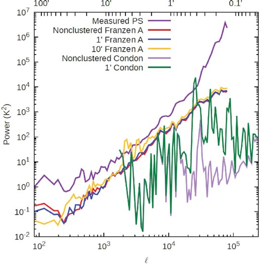
Measured power spectrum (for the coldest patch target field) and the simulated full-pipeline anisotropy power spectrum resulting from (i) the upper limit of potential unremoved point sources down to 100 |$\mu$|Jy according to a point source model presented in Franzen et al. (2016) discussed in Section 3.3, (ii) the upper limit from the same Franzen et al. (2016) model with sinusoidal clustering added on scales of 1 and 10 arcmin, (iii) potential point sources down to nJy fluxes according to the point source model presented in Condon et al. (2012) discussed in Section 4, which can reproduce the surface brightness level of the RSB, and (iv) the same Condon et al. (2012) model with sinusoidal clustering added on a scale of 1 arcmin.

Open in new tabDownload slide

The clustering on a 1-arcmin scale has very little effect on the measured angular power on any angular scale for this model or any of the four. This is because 1 arcmin is considerably less than the average separation of the higher flux sources, which primarily contribute to the measured angular power. In fact, the clustering added in this way on the 1-arcmin scale slightly reduces the angular power on some angular scales because the angular power involves circular averaging, while the sinusoidal variation has been added to essentially rectangular RA and Dec. coordinates at this scale. The 10-arcmin clustering manifests an appreciable increase in angular power on that particular scale. However, this only propagates to some smaller angular scales, and we see from the 1-arcmin clustering case that below a certain angular scale (somewhere between 10 and 1 arcmin), clustering in these models cannot add further angular power.

Given that we clean the images to a flux threshold well below 400 mJy with residuals of only around ∼20 mJy, and that the contribution to the angular power is dominated by the higher flux sources in these models, we emphasize that this modelled observed power resulting from unremoved sources above 100 |$\mu$|Jy is an upper limit and likely a significant overestimate. This indicates that unsubtracted point sources in the images above the flux detection limit are not a major contributor to the measured angular power, and that sources above 100 |$\mu$|Jy generally cannot produce the measured angular power on at least some angular scales.

4 POSSIBLE SOURCE POPULATION

With the angular anisotropy power of the radio sky being larger than that can be accounted for by point sources above 100 |$\mu$|Jy, the question arises as to what flux source count distributions [often denoted by n(S) or |$\frac{{\rm d}n}{{\rm d}{S}}$|] of faint point sources could give rise to the measured angular power. As discussed in Condon et al. (2012), regarding the surface brightness of the RSB, if it is indeed that given by equation (1), then if originating from point sources, given the measured constraints on the source counts above 10 |$\mu$|Jy, those sources must be lower flux and incredibly numerous. We will consider here the possibility that the angular power as well is due to a large number of low-flux point sources.

In a procedure similar to the simulation discussed in Section 3.3, we simulate point source populations distributed in flux according to equation (6) with frequency spectral indices distributed normally around −2.6 in radiometric temperature units with a standard deviation of 0.1 and run the resulting simulated sky through our simulation, imaging, and power spectrum generation pipeline as described there. We adopt the model with the smallest number of sources, which still results in an average around 200 million sources in 1 deg², or 150 sources per pixel. Due to the very large number of sources in this model, computing limitations requires the simulated field of view to be smaller, 0|${_{.}^{\circ}}$|5 on a side, so the calculation of angular power on angular scales larger than this is not possible. The resulting power can still be calculated for most of the range of angular scales of relevance depicted in, for example, Fig. 4. The result for sources distributed randomly in RA and Dec. is shown in Fig. 5. It is seen that because of the very large average number of sources per pixel, the proportional variation in brightness among pixels is small and therefore the resulting angular power in this isotropic model is low. To preliminarily investigate the effects of clustering for this model, we adopt the same simple sinusoidal clustering on a 1-arcmin scale as discussed in Section 3.3, with results also shown in Fig. 5. In this case, with the very large number of sources, the added clustering increases the simulated observed angular power significantly on all angular scales that are equal to and smaller than that of the clustering scale (corresponding in this case to ℓ ∼ 11 000). Thus, we conclude that it is a possibility that with the appropriate clustering on many angular scales over a wide range, the Condon et al. (2012) model of many very low flux sources could reproduce the observed angular power.

5 DISCUSSION

We have carried out a dedicated measurement with LOFAR to determine the anisotropy angular power of the radio background at 140 MHz on angular scales ranging from 2° to 0.2 arcmin. As discussed in Section 2, our results stem from 8 h of observing of two fields with a minimal amount of Galactic diffuse foreground structure. As shown in Section 3, both the direct method of imaging, removing sources, and calculating the power spectrum, and the method of considering the noise per beam in the image with the synthesized beam tapered to a specific width yield a measured angular power that is more than that would result from point sources above 100 |$\mu$|Jy, either distributed randomly spatially or clustered. As shown in Fig. 4, the angular power is also at least an order of magnitude larger than that inferred from measurements at GHz frequencies.

Our measured angular power is around a factor of ∼3 (in the ΔT normalization) lower than that reported by Choudhuri et al. (2020) in the angular scales of overlap (in the range 10² ≤ ℓ ≤ 3 × 10³), applying equation (A12) to convert into the plotted C_ℓ units of their fig. 1. They observe four fields at a variety of Galactic latitudes and longitudes, with all looking through significantly more Galactic structure than the fields in this work. Their reported angular power differs somewhat at various reported ℓ values over their different fields, but this manifests no apparent correlation with the amount of Galactic structure along a line of sight, indicating that the discrepancy between their fields, and more relevantly with the results here, may be due to instrumental effects and analysis considerations. Interestingly, our measured angular power quite closely matches the modelled angular power of unsubtracted point sources below 50 mJy reported in Choudhuri et al. (2020).

The angular power measured here is due to a combination of that due to extragalactic sources, that due to structure in Galactic diffuse emission, and, in principle, that due to possible considerations such as RFI, sidelobe pickup, and residual power from subtracted sources stemming from calibration errors. The lack of artefacts in the visibilities indicates that RFI is not a significant contributor to this measurement, and we do not see evidence of sidelobe pickup in the images, as the sidelobe positions are frequency-dependent and would thus present as shifting patterns in each sub-band. With currently available LOFAR analysis techniques, we cannot absolutely rule out a contribution from the residual power from subtracted sources stemming from calibration errors. In particular, making power spectra at larger scales presents a particular calibration challenge in this regard, as also found by epoch-of-reionization measurements (Barry et al. 2016; Patil et al. 2016; Sadarabadi & Koopmans 2018). Future development of LOFAR analysis techniques may allow a more precise determination of this, but these are beyond the scope of this work.

We can estimate the contribution due to structure in Galactic diffuse emission by noting that the measured angular power in the secondary field is systematically a factor of ∼1.4 higher in the (ΔT)² normalization than that in the coldest patch field, as seen in Fig. 4, and thus a factor of ∼1.2 higher in the (ΔT) normalization. This is, quite tellingly, the same as the square of ratio of the average absolute brightness in radiometric temperature (K) units for the two regions that we calculate using the Haslam et al. (1982) map averaging over pixels within 4° from the field centres (1.2 ± 0.1). As the differences in absolute brightness are due solely to differences in lines of sight through the Galactic diffuse components (as visualized in Fig. 2), this is a strong indication that the proportion of angular power in (ΔT) units due to Galactic structure tracks the proportion of absolute brightness due to that structure, for lines of sight in this general direction of minimal Galactic structure and likely for general lines of sight far away from the Galactic plane. A number of considerations point to the extragalactic component being overwhelmingly dominant (by at least a factor of 5) in terms of the absolute temperature of the background (e.g. Singal et al. 2015) so we believe that the extragalactic component dominates the measured angular power in the coldest patch field by approximately this factor. Stated another way, the normalized angular power |$\left(\frac{\Delta T}{T}\right)$| for both fields is the same, indicating that the contribution to the angular power from Galactic structure is sub-dominant when considering these fields since it is the component that varies spatially between the two fields.

If the angular power measured here is due to low-flux radio point sources, they must be very numerous, paralleling the situation when considering the surface brightness of the radio background. As discussed in Section 4, we simulated the angular power resulting from a source count distribution representing a very large number of sources below 1 |$\mu$|Jy, which, as shown in Condon et al. (2012), could potentially provide the level of surface brightness of the RSB. We found that this source distribution when distributed randomly spatially contains low angular power due to the large number of sources per pixel, but could possibly reproduce the angular power of the RSB measured here given the proper detailed clustering on a wide range of angular scales. It is our intention to continue this modelling in a future work in order to determine the precise clustering parameters for very large numbers of low-flux sources, which could, possibly, result in the angular power spectrum observed here, and to explore the implications of such a population.

ACKNOWLEDGEMENTS

We thank the ‘BAM – Anisotropic Universe 2018’ workshop where initial discussions took place. We acknowledge LOFAR award LC12-005. SHe is supported by NSF Grant No. PHY-1914409. SHo is supported by the U.S. DOE Office of Science under the award number DE-SC0020262 and NSF Grants No. AST-1908960 and No. PHY-1914409. This work was supported by World Premier International Research Center Initiative (WPI), MEXT, Japan. This paper is based on data obtained with the International LOFAR Telescope (ILT) under project code LC12-005. LOFAR (van Haarlem et al. 2013) is the Low-Frequency Array designed and constructed by ASTRON. It has observing, data processing, and data storage facilities in several countries, which are owned by various parties (each with their own funding sources) and which are collectively operated by the ILT foundation under a joint scientific policy. The ILT resources have benefitted from the following recent major funding sources: CNRS-INSU, Observatoire de Paris and Université d’Orléans, France; BMBF, MIWF-NRW, MPG, Germany; Science Foundation Ireland (SFI), Department of Business, Enterprise and Innovation (DBEI), Ireland; NWO, the Netherlands; and the Science and Technology Facilities Council, UK.

DATA AVAILABILITY

The data underlying this paper will be shared on reasonable request to the corresponding author.

Footnotes

REFERENCES

APPENDIX A: RELATIONS BETWEEN MEASURES OF ANGULAR POWER OF TEMPERATURE ANISOTROPIES

In this appendix, we present the scaling relationships between two normalizations for the angular power of temperature anisotropies, and derive which arises naturally from power spectra obtained from interferometric observations.

A1 Power spectrum normalizations and multipole moments

Note on notation and dimensions: Square brackets [ ] will indicate ‘dimensions of’. Here, in order to keep track of factors of the angular scale ℓ and normalization factors of π in quantities, we will follow factors of ℓ and π by a quasi-dimensionality. That is, to encompass both dimensions with physical units and these normalization factors, we will refer in this work to ‘quasi-dimensionality’ to encapsulate both. Definitions of relevant quantities have been obtained from Ryden (2006), Lesgourgues (2013), and Jackson (1998).

A2 Power spectra from interferometric observations