


ABSTRACT
We estimate the 3D density profile of the Galactic dark matter (DM) halo within r ≲ 30 kpc from the Galactic centre by using the astrometric data for halo RR Lyrae stars from Gaia DR2. We model both the stellar halo distribution function and the Galactic potential, fully taking into account the survey selection function, the observational errors, and the missing line-of-sight velocity data for RR Lyrae stars. With a Bayesian method, we infer the model parameters, including the density flattening of the DM halo q, which is assumed to be constant as a function of radius. We find that 99 per cent of the posterior distribution of q is located at q > 0.963, which strongly disfavours a flattened DM halo. We cannot draw any conclusions as to whether the Galactic DM halo at |$r \lesssim 30 \, \mathrm{kpc}$| is prolate, because we restrict ourselves to axisymmetric oblate halo models with q ≤ 1. Our DM density profile might be biased especially in the inner few kpc, due to the uncertainty in the baryonic distribution. Our result is in tension with predictions from cosmological hydrodynamical simulations that advocate more oblate (〈q〉 ∼ 0.8 ± 0.15) DM haloes within |${\sim}15{{\ \rm per\ cent}}$| of the virial radius for Milky-Way-sized galaxies. An alternative possibility, based on our validation tests with a cosmological simulation, is that the true value q of the Galactic halo could be consistent with cosmological simulations but that disequilibrium in the Milky Way potential is inflating our measurement of q by 0.1–0.2. As a by-product, our model constrains the DM density in the Solar neighbourhood to be |$\rho _{\mathrm{DM},\odot } = (9.01^{+0.18}_{-0.20})\times 10^{-3}{\,\rm M_\odot} \mathrm{pc}^{-3} = 0.342^{+0.007}_{-0.007}$| GeVcm−3, consistent with other recent measurements.
1 INTRODUCTION
Determining the mass distribution of the dark matter (DM) halo of the Milky Way (MW) is currently one of the most important tasks in Galactic astronomy in the cosmological context, because the shape of the Galactic DM halo can be used to test the prediction from Lambda cold dark matter (ΛCDM) cosmology.
There have been numerous efforts to measure the density profiles and shapes of DM haloes arising from cosmological N-body simulations. DM-only simulations show that the spherically averaged radial density profiles of DM haloes follow a universal form (Navarro, Frenk & White 1997) and that their three-dimensional (3D) mass distributions are triaxial (Jing & Suto 2002). It has also been recognized that the DM halo’s shape is affected by the infall and condensation of baryons (Dubinski 1994; Kazantzidis et al. 2004; Kazantzidis, Abadi & Navarro 2010; Zemp et al. 2012; Zhu et al. 2016). This result has recently been confirmed on 10 000 haloes with masses in the range 1011−3 × 10¹⁴M⊙ from the Illustris suite of simulations with and without baryonic physics (Chua et al. 2019). In particular, DM haloes of MW-sized galaxies with baryons have a nearly oblate axisymmetric shape, with a minor-to-major axial ratio of 0.79 ± 0.15, especially within 0.15r200. (Here, r200 is the virial radius within which the average density is 200 times the critical density of the Universe.) In contrast, DM-only simulations in the same mass range have DM haloes that are highly triaxial. A similar trend is also reported by Prada et al. (2019), who used MW-sized haloes in Auriga simulations. The deformation of the DM haloes by the baryons has been shown to arise due to the deformation in the shapes of the orbits of DM particles by the more concentrated baryonic components in both controlled and cosmological simulations (Debattista et al. 2008; Valluri et al. 2010, 2012).
In summary cosmological hydrodynamical simulations over the past two decades have consistently predicted that the DM haloes of MW-sized galaxies are nearly oblate-axisymmetric especially in the inner regions (<30–|$50 \, \mathrm{kpc}$|), becoming more triaxial at larger radii.
In this paper, we test this prediction by measuring the mass distribution of the Galactic DM halo using halo stars as kinematic tracers of the 3D mass distribution of the MW halo.
There are two broad categories of methods that have frequently been used to measure the shape of the MW’s DM halo.1 The first uses the kinematics and spatial distribution of stellar streams in the halo (Johnston et al. 1999; Helmi 2004; Johnston, Law & Majewski 2005; Fellhauer et al. 2006; Koposov, Rix & Hogg 2010; Law & Majewski 2010; Sanders & Binney 2013; Bovy 2014; Gibbons, Belokurov & Evans 2014; Bowden, Belokurov & Evans 2015; Küpper et al. 2015; Bovy et al. 2016; Malhan & Ibata 2019; Vasiliev, Belokurov & Erkal 2021). This method relies on the fact that stellar streams are remnants of tidally disrupted dwarf galaxies or star clusters, and that stars that form the stellar stream have coherent motions and show a 1D spatial distribution that approximately traces the orbit of the progenitor system.
The second method is to use the kinematics of halo tracers such as globular clusters or halo field stars. In this approach, the halo tracers are assumed to be in dynamical equilibrium, and the task is to determine the Galactic potential such that the observed position and velocity of halo tracers are consistent with this equilibrium assumption. Many of the previous studies used the axisymmetric form of the Jeans equations (Loebman et al. 2014; Bowden, Evans & Williams 2016; Eadie & Jurić 2019; Wegg, Gerhard & Bieth 2019; Nitschai, Cappellari & Neumayer 2020). Motivated by the availability of accurate astrometric data from Gaia DR2 (Lindegren et al. 2018), there have been several attempts to model the positions and velocities of halo tracers with the phase-space distribution function (DF) fitting (McMillan & Binney 2012, 2013; Binney & Piffl 2015; Cole & Binney 2017; Posti & Helmi 2019). Our work is a continuation of these latter works, and we use DF models to infer the Galactic potential.
In this paper, we infer the 3D mass distribution of the Galactic DM halo by simultaneously modelling the DF of the halo stars and the MW potential. The ‘DF fitting’ technique was pioneered by McMillan & Binney (2012), McMillan & Binney (2013) and extended by Ting et al. (2013), Bovy & Rix (2013) and Trick, Bovy & Rix (2016). The most important improvement of our implementation of this method is that we explicitly take into account distance errors in a computationally tractable way, which were neglected in previous works (McMillan & Binney 2012, 2013).
In previous works of a similar nature, Das & Binney (2016) and Das, Williams & Binney (2016) modelled the stellar halo DF (and its metallicity dependence) while keeping the MW potential fixed. Also, Binney & Piffl (2015) and Cole & Binney (2017) modelled the DF of the DM halo, while we only model the spatial density distribution of the DM halo.
The outline of this paper is as follows. In Section 2, we describe the data sets used in this paper. In Section 3, we describe our model ingredients. In Section 4, we describe how we evaluate the likelihood function from the stellar halo data. In Section 5, we describe the setup for our Bayesian analysis. In Section 6, we present our results. In Section 7, we compare our results with the literature in this field and we mention some issues in our analysis. In Section 8, we present our conclusion.
In Appendix D, we present validation tests of our method on a variety of mock stellar halo data.
2 DATA
Here, we describe three sets of kinematic data used in this paper. We note that the coordinate system is defined in Appendix A.
2.1 Circular velocity
The best way of constraining the Galactic potential in the disc plane is to use the circular velocity vcirc(R). In our analysis, we use the measurement of vcirc(R) between |$5 \le R \le 25\, \mathrm{kpc}$| from Eilers et al. (2019). This measurement was obtained by applying Jeans analysis to 6D phase-space coordinates for more than 23 000 disc red giants with photometric data from 2MASS, WISE, and Gaia DR2 for which precise spectrophotometric distances were derived from APOGEE DR14 (Hogg, Eilers & Rix 2019).
Due to accurate distances, the uncertainty in vcirc is small in Eilers et al. (2019). The random error is σcirc,rand ≃ (1–3) |$\, \mathrm{km\ s}^{-1}$| at |$R \lesssim 20 \, \mathrm{kpc}$|, and |$\sigma _\mathrm{circ,rand} \sim 10 \, \mathrm{km\ s}^{-1}$| at |$20 \, \mathrm{kpc}\le R \le 25 \, \mathrm{kpc}$|. The systematic error is roughly σcirc,sys ≃ (0.02–0.05) × vcirc. The quoted systematic error arises from various assumptions in the way they performed the Jeans analysis, such as the assumed density profile of the stellar disc. We do not take into account the systematic error in our fiducial analysis, but we have verified that the inclusion of the systematic error hardly changes our main conclusions.
2.2 Vertical force Kz at z = 1.1 kpc
Classically, the vertical component of the force at |$z=1.1 \, \mathrm{kpc}$| away from the disc plane, |$K_{z, 1.1 \, \mathrm{kpc}} (R)$|, has been measured via the vertical Jeans equation (Kuijken & Gilmore 1991). We use a recent measurement of |$K_{z, 1.1 \, \mathrm{kpc}}(R)$| by Bovy & Rix (2013) to aid our measurement of the gravitational potential. To be specific, we used the values of R − R0 and |$K_{z, 1.1 \, \mathrm{kpc}}(R)$| in their table 3, by adopting |$R_0 = 8.178 \, \mathrm{kpc}$| (Gravity Collaboration 2019).
We note that Bovy & Rix (2013) derived |$K_{z, 1.1 \, \mathrm{kpc}}(R)$| by analysing the DFs of various mono-abundance populations in the thin and thick discs of the Milky Way from SDSS/SEGUE data. Thus, their data are independent of the halo RR Lyrae data discussed in Section 2.3. Also, while the circular velocity data (discussed in Section 2.1) constraints the radial force in the Galactic disc plane, |$K_{z, 1.1 \, \mathrm{kpc}}(R)$| constraints the vertical force measured at a small distance away from the disc plane. In this regard, vcirc and the |$K_{z, 1.1 \, \mathrm{kpc}}$| are complementary data.
2.3 The RR Lyrae sample: 5D phase-space coordinates
2.3.1 Sample selection
To measure the global 3D shape of the Galactic potential, we need kinematic data for halo tracers. We use the ‘clean’ sample of 93,345 RR Lyrae stars compiled by Iorio & Belokurov (2019) (and kindly provided by Dr. Giuliano Iorio), which were selected from the Gaia DR2 catalogue. This sample does not include stars associated with known halo substructure (such as the core of the Sagittarius stream, satellite galaxies, or globular clusters).2
2.3.2 Content of the RR Lyrae sample
In this paper, we neglect the errors in (ℓ, b). In our RR Lyrae catalogue, the distance is estimated from period–luminosity relationship. The uncertainty in the distance modulus is quite uniform, with |$\sigma _{\mathcal {D}} = 0.2401 \pm 0.0056$| (the fractional distance error is 11.07 ± 0.26 per cent; Iorio & Belokurov 2019). Thus, in our analysis, we assume that the errors in |$\mathcal {D}$| are |$\sigma _{\mathcal {D}} = 0.240$| for all the stars. This assumption of uniform error in |$\mathcal {D}$| plays an important role in simplifying our DF fitting (see Section 4.3.1).
3 MODEL
Our goal is to estimate the density of the DM halo, ρDM(R, z). To achieve this goal, we use parametric models for the (1) MW potential Φ(R, z) (consisting of baryonic and DM components); and (2) stellar halo DF |$f(\rm{\boldsymbol {J}})$| and estimate the parameters of these components with a Bayesian analysis. Throughout this paper, we assume that the MW is static and axisymmetric, and that the stellar halo is in dynamical equilibrium. While this assumption has been recently called into question by modelling of tidal streams (Erkal et al. 2019; Vasiliev et al. 2021) and the kinematics of outer halo stars (Petersen & Peñarrubia 2021), in this paper (as in most works that use distributed field halo stars as kinematic tracers) we ignore this disequilibrium, but we test this assumption in a follow-up paper (de Salas et al., in preparation).
In this section, we describe the ingredients of our equilibrium model. All the parameters in our analysis are summarized in Table 1.
Bayesian prior and posterior distributions of our model parameters and the best-fitting parameters in our fiducial analysis with RR Lyrae stars.
| Parameter | Quantity | Prior distribution | Note | Posterior distribution | Best fitting |
|---|---|---|---|---|---|
| MW potential | |||||
| Free | Mbulge (bulge mass) | Mbulge = (8.9 ± 0.89) × 109 M⊙ | (1) | [8.33, 9.23, 10.09] × 109 M⊙ | 9.53 × 10⁹ M⊙ |
| Free | Mthin (thin disc mass) | Mthin = (35 ± 10) × 109 M⊙ | (2) | [34.39, 36.53, 38.55] × 109 M⊙ | 37.22 × 10⁹ M⊙ |
| Free | Mthick (thick disc mass) | Mthick = (6 ± 3) × 109 M⊙ | (2) | [4.45, 6.21, 8.59] × 109 M⊙ | 7.30 × 10⁹ M⊙ |
| Free | |$R_\mathrm{d}^\mathrm{thin}$| (thin disc scale radius) | |$R_\mathrm{d}^\mathrm{thin}= (2.6\pm 0.5) \, \mathrm{kpc}$| | (2) | |$[2.58, 2.68, 2.80] \, \mathrm{kpc}$| | |$2.63 \, \mathrm{kpc}$| |
| Free | |$R_\mathrm{d}^\mathrm{thick}$| (thick disc scale radius) | |$R_\mathrm{d}^\mathrm{thick}= (2.0\pm 0.2) \, \mathrm{kpc}$| | (2) | |$[1.76, 1.96, 2.15] \, \mathrm{kpc}$| | |$1.94 \, \mathrm{kpc}$| |
| Fixed | |$z_\mathrm{d}^\mathrm{thin}$| (thin disc scale height) | |$z_\mathrm{d}^\mathrm{thin}= 0.3 \, \mathrm{kpc}$| (fixed) | (1) | |$0.3 \, \mathrm{kpc}$| (fixed) | ... |
| Fixed | |$z_\mathrm{d}^\mathrm{thick}$| (thick disc scale height) | |$z_\mathrm{d}^\mathrm{thick}= 0.9 \, \mathrm{kpc}$| (fixed) | (1) | |$0.9 \, \mathrm{kpc}$| (fixed) | ... |
| Free | q (DM density flattening) | Flat at 0.2 < U ≤ 0.5 (oblate) | (3) | [0.983, 0.993, 0.998] | 0.996 |
| Free | γ (DM inner density slope) | Flat at 0 < γ < 1.9 | ... | [0.785, 0.982, 1.209] | 0.738 |
| Free | a (DM scale radius) | Flat at −∞ < log10a < ∞ | ... | |$[10.29, 12.49, 16.66] \, \mathrm{kpc}$| | |$10.46 \, \mathrm{kpc}$| |
| Free | log10ρ0 (DM normalization) | Flat at −∞ < log10ρ0 < ∞ | ... | [6.89, 7.21, 7.44] | 7.44 |
| ... | Thick to thin disk ratio | Σthick(R0)/Σthin(R0) = (0.12 ± 0.04) | (2) | [0.070, 0.104, 0.139] | 0.120 |
| ... | Total stellar mass | Equation (9) | (2) | [50.13, 52.32, 54.24] × 109 M⊙ | 54.04 × 10⁹ M⊙ |
| ... | Dark matter concentration c′ | |$\ln c^{\prime }_\mathrm{v} = \ln (r_{94}/r_{-2}) = 2.56 \pm 0.272$| | (2) | [18.45, 19.55, 20.89] | 18.87 |
| Stellar halo DF | |||||
| Free | ain (inner velocity anisotropy) | Flat at 0 < ain < 1. | (4) | [0.234, 0.404, 0.649] | 0.331 |
| Free | bin (inner velocity anisotropy) | Flat at 0 < bin < 1. | (4) | [0.789, 0.879, 0.921] | 0.890 |
| Free | aout (outer velocity anisotropy) | Flat at 0 < aout < 1. | (4) | [0.292, 0.342, 0.383] | 0.346 |
| Free | bout (outer velocity anisotropy) | Flat at 0 < bout < 1. | (4) | [0.792, 0.836, 0.861] | 0.842 |
| Free | log10J0 (Action scale in DF) | Flat at −∞ < log10J0 < ∞ | ... | [3.02, 3.22, 3.59] | 3.25 |
| Free | Γ (inner halo density index) | Flat at 0 ≤ Γ < 2.8 | ... | [0.49, 1.47, 2.47] | 1.50 |
| Fixed | B (outer halo density index) | Fixed to B = 5 | (5) | 5 (fixed) | ... |
| Fixed | κ (halo rotation) | Fixed to κ = 0 (non-rotating) | (6) | 0 (fixed) | ... |
| Fixed | Jϕ,0 (action scale in DF) | Fixed to Jϕ,0 = const. | (6) | const. (fixed) | ... |
| Free | log10η (outlier fraction) | Flat at −∞ < log10η < −2 | ... | [−7.26, −4.65, −3.21] | −3.99 |
Note. (1) – The same prior as in McMillan (2017). (2) – The prior is taken from the data compiled in Bland-Hawthorn & Gerhard (2016). See Section 5.2. (3) – U = (2/|$\pi$|)arctan(q) (equation 8). The range of 0.2 < U ≤ 0.5 corresponds to 0.3249 < q ≤ 1. (4) – See equation (14). (5) – We fix the parameter B = 5, as it cannot be well constrained by our inner halo sample. (6) – (κ, Jϕ,0) are fixed in this paper, except for the mock analysis with mock data generated from a cosmological simulation (see Appendix D2.4).
3.1 Models for the gravitational potential
We model Φ(R, z) following the parametrization by McMillan (2017), except that we allow the DM distribution to be oblate-axisymmetric rather than spherical. First, we briefly summarize the functional forms assumed for the baryonic mass components (the bulge, stellar discs, and gas discs) which are identical to McMillan (2017). In addition, most of the parameters of the baryonic potential are also fixed to the best-fitting parameters in McMillan (2017). We then describe our assumed DM distribution model.
3.1.1 The bulge
3.1.2 The thin and thick stellar discs
3.1.3 The atomic and molecular gas discs
3.1.4 The dark matter halo
As we shall describe in Section 3.1.5, we do not allow prolate DM distributions. Thus, we use a flat prior for U: 0.2 < U ≤ 0.5. (This range of U corresponds to 0.3249 < q ≤ 1.) The prior for (γ, a, ρ0) are shown in Table 1.
We use similar definitions for the concentration parameter, virial mass, and virial radius to those in McMillan (2017), by evaluating these quantities by spherically averaging the non-spherical density. Namely, for a given set of parameters (ρ0, γ, a, q), we define two radii r200 and r94 such that the mean density within a sphere of r200 and r94 is 200 and 94 times the critical density (|$\rho _\mathrm{crit} = 137.55 {\,\rm M_\odot} \, \mathrm{kpc}^{-3})$|; see Binney & Tremaine 2008), respectively. The virial mass M200 and M94 are defined as the enclosed mass within the sphere of radius r200 and r94, respectively. We define 〈ρ(r)〉 as the mean density within a spherical shell centred at a radius r; and we define the radius r−2 such that dln 〈ρ〉/dln r = −2. The concentration parameter is defined as |$c^{\prime }_\mathrm{v} = r_{94}/r_{-2}$|.
3.1.5 A note on the oblate assumption of the dark matter halo
Throughout this paper, we only consider q ≤ 1, because the current version of AGAMA (Vasiliev 2019) that is used in our paper only allows computation of orbital actions in oblate (or spherical) potentials. This limitation is inherent to the Stäckel fudge method (Binney 2012) and stems from a more complex orbital structure of prolate potentials, which support two different long-axis tube orbit classes.
In computing the radial and vertical action of a given star with the Stäckel fudge method, it is essential to define an adequate ellipsoidal coordinate (λ, μ) in the (R, z) plane, such that the orbital motion of the star in (R, z) plane is approximately bounded by two λ = constant curves and two μ = constant curves (Binney 2012; Sanders & Binney 2015a, 2016; Vasiliev 2019). When the MW potential is oblate axisymmetric, such an ellipsoidal coordinate has the foci on the z-axis (i.e. prolate coordinate system is needed for an oblate potential). However, if the MW potential is prolate axisymmetric, due to the orbital geometry allowed in the prolate systems, the foci are located on the R-axis. The current version of AGAMA only supports the ellipsoidal coordinate for which foci are on the z-axis (i.e. valid only in oblate potentials). Therefore, using the current version of AGAMA to compute radial or vertical action in prolate system is mathematically incorrect. We note that some studies including Posti & Helmi (2019) did not take this limitation into account although they used AGAMA.
3.2 Distribution function model
3.2.1 Action-based distribution function
The parameter J0 implicitly determines the break radius, where these halo properties gradually change from the inner to the outer asymptotic values (the relation between J0 and the actual radius depends on the potential). We adopt a flat prior on log10J0.
The parameter Γ(<3) and B(>3) govern the inner and outer density slope of the stellar halo, respectively.3 For the prior on Γ, we adopt a flat prior at Γ at 0 ≤ Γ < 2.8. The parameter B is fixed to B = 5 in our analysis (cf. Binney & Wong 2017), because it is difficult to constrain B (or, roughly speaking the outer density profile) with our inner halo data at |$5 \lesssim r/\, \mathrm{kpc}\lesssim 27.5$|.
The parameter κ determines the net rotation of the stellar halo and Jϕ,0 determines the scale of the angular momentum under which the rotation is suppressed. In the fiducial analysis with the Gaia RR Lyrae stars, we set κ = 0 and set Jϕ,0 to be some constant. This is because we observe little net rotation for 1022 RR Lyrae stars within our survey volume with full 3D velocity data.4
To summarize, in analysing the Gaia RR Lyrae sample, we treat the following parameters as free parameters for the action-based DF fmain: The ‘break radius’ action J0, the parameter governing the inner stellar halo density Γ, and the quantities governing the velocity anisotropy (ain, bin, aout, bout). Other parameters are fixed, as shown in Table 1.
3.2.2 Simple distribution function for the outlier population
3.3 Selection function model
3.4 Error model
4 LIKELIHOOD OF THE STELLAR HALO DATA
As mentioned in Section 3, the objective of our analysis is to fit the kinematic data for RR Lyrae stars with a DF model. Here, we derive the likelihood for the RR Lyrae data given a set of model parameters.
The likelihood function we adopt is similar to those that have already been derived and discussed in previous studies (most notably McMillan & Binney 2012, 2013; Trick et al. 2016). However, these previous derivations ignore, or do not properly consider, the observational errors in distances to stars. We propose a new approach to handling the distance errors by taking advantage of the fact that all the RR Lyrae stars in our sample have approximately the same error on distance modulus.
For completeness, we start our discussion from the case where the stellar sample is error-free. Then, we proceed to a more realistic case in which observational errors (including distance errors and missing line-of-sight velocities) are taken into account.
4.1 Formulation with error-free data
4.2 Formulation with observational errors
In the presence of the observational errors, the expression for the probability |$\mathrm{Pr} (\rm{\boldsymbol {x}}_i, \rm{\boldsymbol {v}}_i | M)$| becomes more complicated, as pointed out by Trick et al. (2016).6 We introduce a function |$E(\rm{\boldsymbol {u}} | \rm{\boldsymbol {u}}^{\prime } , M)$| that denotes the probability that a star’s observable vector is |$\rm{\boldsymbol {u}}$| given its true vector |$\rm{\boldsymbol {u}}^{\prime }$| and the model M. (Remember our notation that a primed quantity such as |$\rm{\boldsymbol {u}}^{\prime }$| denotes the true value of an unprimed quantity; see Section 3.4.)
4.3 Evaluation of equation (27) for the RR Lyrae sample
The result of equation (27) is generally applicable to both 6D data and 5D data, including our RR Lyrae sample with missing vlos. This is because 5D data without vlos data is equivalent to 6D data with large observational errors in vlos (McMillan & Binney 2013). In the following, we will show how to evaluate |$\mathrm{Pr} (\bar{\rm{\boldsymbol {u}}}_i | M)$| in equation (27) for our RR Lyrae sample.
4.3.1 Denominator in equation (27)
In general, |$\sigma _{\mathcal {D}}$| is non-zero and each star has a different value of |$\sigma _{\mathcal {D}}$|. In such a case, we need to evaluate A for each star, which is computationally very expensive. This is why |$\sigma _{\mathcal {D}}$| is neglected (or explicitly set to be zero) in previous studies (McMillan & Binney 2013; Trick et al. 2016). However, if |$\sigma _{\mathcal {D}}$| is approximately the same for the entire sample, which is the case for our RR Lyrae stars, we need to evaluate A only once for a given model, by assuming a single value for |$\sigma _{\mathcal {D}}$|. With this prescription, we can dramatically reduce the computational cost while keeping our likelihood evaluation more precise. The derivation of equations (29) and (30) is the most important improvement we have over the previous formulation by McMillan & Binney (2013) and Trick et al. (2016).
4.3.2 Numerator in equation (27)
The numerator of equation (27) can be numerically evaluated using Monte Carlo integration.
4.4 Likelihood of the RR Lyrae stars
4.4.1 Numerical evaluation of the total likelihood
Our goal is to combine the likelihood of the RR Lyrae data given model M, ln L(Data(RRL)|M), with the likelihood functions of the circular velocity data and the vertical force data for our Markov chain Monte Carlo (MCMC) analysis. Thus, we need to be careful so that the numerical noise in the likelihood will not seriously affect our inference of the model parameters. Here, we focus on the 5D case and we describe two important numerical techniques to achieve our goal.
The first technique is related to the Monte Carlo integration of equation (33). The precision of this integration is determined by the number of Monte Carlo samples, NMC. Ideally, it is desirable to set NMC as large as possible to minimize the numerical noise in |$\mathrm{Pr} (\bar{\rm{\boldsymbol {u}}}_i | M)$|. However, this requires a large computational cost although we are not specifically interested in the absolute value of |$\mathrm{Pr} (\bar{\rm{\boldsymbol {u}}}_i | M)$|. Rather, we are more interested in the relative value of |$\mathrm{Pr} (\bar{\rm{\boldsymbol {u}}}_i | M)$| for different models (e.g. M = M1 and M = M2). Thus, following McMillan & Binney (2013), we use the same set of sampling points |$\rm{\boldsymbol {u}}^{\prime }_{ij}$| and weights wij throughout our MCMC analysis. We find that NMC = 100 is enough for our purpose.
The second technique is related to the evaluation of A in equation (35). As discussed in Section 4.3.1, the value of A is common for all the RR Lyrae stars. If the fractional error in A is ϵ (ϵ ≪ 1), then this error results in an error of δ(log10L(Data(RRL)|M)) = (1/ln 10)NRRL,effϵ = 0.43NRRL,effϵ (see discussion in McMillan & Binney 2013). If we require a tolerance of δ(log10L) < 0.5, then the fractional error in A has to satisfy ϵ < (0.5/ln 10)/NRRL,eff = 1/(0.87NRRL,eff). With unlimited computational resources, we could have set NRRL,eff = 16197(= NRRL). However, the evaluation of A (see equation 29) is computationally challenging, because it involves 6D integration in the phase-space of observable quantities and the conversion of observable quantities into actions. We use an adaptive multidimensional integration package, cubature (https://github.com/stevengj/cubature), to evaluate A, and find that even with this sophisticated package, the integration does not converge within 10 min per model8 if we set NRRL,eff = NRRL. After some experiments, we find that setting NRRL,eff = 1000 (or NRRL,eff ≤ 3000) is a reasonable choice for our analysis in terms of the computational speed and numerical accuracy. Mathematically, setting NRRL,eff < NRRL is equivalent to assigning a weight of (NRRL,eff/NRRL) to each of our RR Lyrae stars. As a result, the constraining power from our RR Lyrae star sample is reduced, as if we only had NRRL,eff stars in our catalogue.
5 ANALYSIS
5.1 Bayesian likelihood
5.1.1 Likelihood of the circular velocity data
5.1.2 Likelihood of the vertical force data
5.1.3 Total likelihood of the data
5.2 Bayesian prior
Our Bayesian prior for the MW potential and the stellar halo DF is described in Sections 3.1 and 3.2, respectively. These priors are summarized in Table 1. We note that the prior distributions for the parameters of the model potential are mostly taken from Bland-Hawthorn & Gerhard (2016) and McMillan (2017). We have tried various prior distributions and confirmed that the choice of the prior distribution does not change the main conclusion of our paper, especially the flattening of the DM halo.
5.3 Markov chain Monte Carlo analysis
To estimate the model parameters, we first search for the maximum-likelihood parameters with a Nelder-Mead optimization package constrNMPy (https://github.com/alexblaessle/constrNMPy) with some reasonable tolerance level. Then we use the resultant parameters as the initial condition of the Bayesian MCMC analysis. We use a package emcee (Foreman-Mackey et al. 2013) for the MCMC analysis. We use (2 × Nfree) walkers (where Nfree is the number of free parameters) and run the MCMC for several thousand steps. We discard initial half of the chain for burn-in and analysed the remaining chain.
The analysis code is written in python, and it is developed from an example code in AGAMA (https://github.com/GalacticDynamics-Oxford/Agama/blob/master/py/example_df_fit.py). In Appendix D, we validate our method with mock data sets.
6 RESULTS
In this section, we describe the results of our Bayesian MCMC analysis. The posterior distribution is summarized in Table 1. The corner plots are given in Appendix B.
6.1 Comparison of the input data and our model
To check the performance of our method, we first compare the input data and our model predictions.
6.1.1 Circular velocity
Fig. 2 shows the radial profile of the circular velocity vcirc(R) and the contribution from baryonic and DM components sampled from our posterior distribution. We can see that our model properly fits the rotation curve data from Eilers et al. (2019).
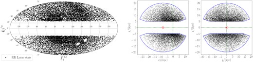
Distribution of the 16 197 stars in our RR Lyrae sample on the sky (left-hand panel), in the Galactocentric Cartesian (x, z)-plane (middle panel) and (y, z)-plane (right-hand panel). Our sample does not include stars associated with obvious substructure, such as the Large and Small Magellanic Clouds (two small holes in the left-hand panel at around 270○ < ℓ < 315○, −50○ < b < −25○). In the middle- and right-hand panels, the Solar location is marked with the red ⊙ symbol. Our sample selection criteria only select stars that are confined within the region enclosed by the solid blue curve.
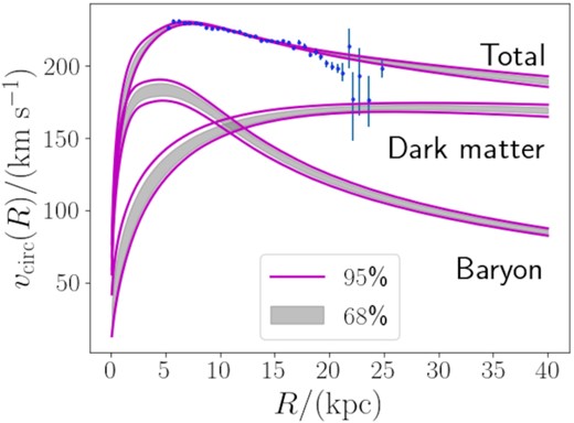
The radial profile of the circular velocity vcirc(R), along with its contribution from baryon and DM. The grey shaded region corresponds to the central 68 percentile of the posterior distribution of our model, while the magenta solid lines cover the central 95 percentile. The blue data points with error bar are taken from Eilers et al. (2019), which are one of the input data sets for our fit.
We note that the vcirc data used in our study (Eilers et al. 2019) were also analysed in Eilers et al. (2019) and de Salas et al. (2019) to estimate the DM density profile. Both of these studies found a reasonable model that fits the input data. de Salas et al. (2019) pointed out that a good fit to the vcirc data can be achieved by assuming different functional forms of the baryonic potential. This result suggests that a wide variety of baryonic models can explain the vcirc data equally well. Therefore, it is not surprising that we arrived at a good fit to the vcirc data. de Salas et al. (2019) also found that the posterior distribution of the parameters in their baryonic model potentials, such as the mass and the scale radius of the bulge or the stellar disc, are dominated by the prior distribution. This result implies that the circular velocity data alone are not good enough to constrain all the parameters of the potential. Similar to their finding, we found that the posterior distributions of the parameters for the bulge and the thick disc are dominated by the priors when we used the vcirc data plus Kz data (with or without the RR Lyrae data) (see Fig. C1). Our result confirms that a proper modelling of the baryonic mass model and a well-determined prior information on the parameters for the baryonic mass model are essential to make an inference on the MW potential.
6.1.2 Vertical force
Fig. 3 shows the radial profile of the vertical force |$K_{z,1.1\, \mathrm{kpc}}$| sampled from our posterior distribution. We can see that our model properly fits the data points of Bovy & Rix (2013). Our posterior distribution suggests that the local value of |$K_{z,1.1\, \mathrm{kpc}}$| measured at |$R=R_0=8.178 \, \mathrm{kpc}$| (Gravity Collaboration 2019) is |$K_{z,1.1\, \mathrm{kpc}}(R_0) = (72.7 \pm 1.4) / (2\pi G {\,\rm M_\odot} \, \mathrm{pc}^{-2})$|, which is consistent with the classical measurement of |$(71 \pm 6) / (2\pi G {\,\rm M_\odot} \, \mathrm{kpc}^{-2})$| by Kuijken & Gilmore (1991).
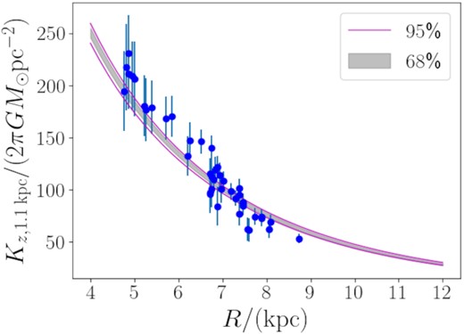
The radial profile of the vertical force |$K_{z, 1.1 \, \mathrm{kpc}}$| measured at |$z=1.1 \, \mathrm{kpc}$|. The grey shaded region corresponds to the central 68 percentile of the posterior distribution of our model, while the magenta solid lines cover the central 95 percentile. The blue data points with error bar are taken from Bovy & Rix (2013), which are one of the input data sets for our fit.
6.1.3 Proper motion distribution
In the left-hand hand column of Fig. 4, we show the statistical properties of the proper motion distribution, |$(\rho _{\mu _{\ell *}, \mu _{b}}, \sigma _{\mu _{\ell *}}, \sigma _{\mu _{b}})$|, as a function of (ℓ, b) for our RR Lyrae sample. In computing these quantities, we first divide the RR Lyrae star sample into 72 × 18 cells with a size of (Δℓ, Δb) = (5○, 10○). Then, we analyse the proper motion distribution in each cell to evaluate |$(\rho _{\mu _{\ell *}, \mu _{b}}, \sigma _{\mu _{\ell *}}, \sigma _{\mu _{b}})$|.9
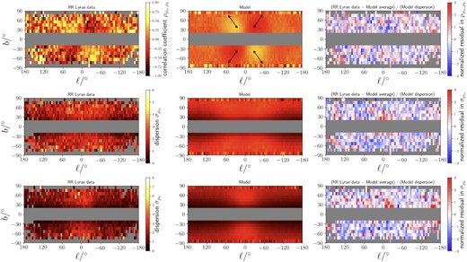
A visualization of the proper motion distribution of our RR Lyrae sample (left-hand column), the average prediction of our models constructed from the MCMC chain (middle column), and the normalized residual between data and model (right-hand column). In the top row, we show the result for the Pearson correlation coefficient |$\rho _{\mu _{\ell *}, \mu _b}$| for the distribution of 2D proper motion (μℓ*, μb). As shown by the arrows in the top-middle panel, the quadrupole pattern of the |$\rho _{\mu _{\ell *}, \mu _b}$| on the sky corresponds to a preferential motion of the RR Lyrae stars with radial orbits. In the middle row, we show the result for the dispersion |$\sigma _{\mu _{\ell *}}$| of the distribution of μℓ,*. In the bottom row, we show the result for the dispersion |$\sigma _{\mu _{b}}$| of the distribution of μb.
In the middle column of Fig. 4, we also derive the same statistical properties by using the posterior distribution. First, we randomly select 160 models from our MCMC chain. For each model, we generate a large enough sample of mock stars from the DF, and add the observational uncertainty. Then we randomly select 16197 error-added mock stars within the survey volume as in our RR Lyrae sample. We compute |$(\rho _{\mu _{\ell *}, \mu _{b}}, \sigma _{\mu _{\ell *}}, \sigma _{\mu _{b}})$| for each model, and average these quantities over 160 models along each line of sight.
In the right-hand column of Fig. 4, we show the normalized difference between the data and our models for each of the statistical properties of the proper motion distribution. Here, we first computed the average and the dispersion of the above-mentioned 160 models. Then, for each line of sight, we computed the residual between the data and average divided by the dispersion.
We see that the overall trend in the proper motion distribution is well recovered by our models. At −90○ < ℓ < 90○ and −90○ < b < 90○, we can see the quadrupole pattern in the correlation coefficient |$\rho _{\mu _{\ell *}, \mu _{b}}$| in the top row of Fig. 4 for both the RR Lyrae sample and our models. This pattern is known to be a characteristic of a radially biased velocity distribution (Iorio & Belokurov 2019). To illustrate this feature, we put four arrows in the top middle panel that describe how radial-orbit stars approximately move when seen from the Sun. The orientation of these arrows matches the quadrupole pattern of |$\rho _{\mu _{\ell *}, \mu _{b}}$|. We note that it is the first time this proper motion distribution is successfully fit and recovered by a DF model. The model distributions for the dispersion |$\sigma _{\mu _l*}$| and |$\sigma _{\mu _b}$| in the next two rows also show very good overall agreement.
6.2 Comparison of the external data and our DF model
In this section, we compare our results with other independent data sets that are not used to constrain our model. This comparison serves to test the predictive power of our model.
In Fig. 5, we show the radial profile of the 3D velocity dispersion (σr, σθ, σϕ) and the velocity anisotropy |$\beta = 1 - (\sigma _\theta ^2+\sigma _\phi ^2)/(2\sigma _r^2)$| for halo K giants obtained by the LAMOST survey (Bird et al. 2019). These data (shown as coloured open symbols) are not used in our analysis, but are compared with our model predictions (solid and dashed lines).

Top panel: The radial profile of the velocity dispersion σr (red), σθ (green), and σϕ (blue) as a function of r predicted by our models. Bottom panel: The corresponding radial profile of velocity anisotropy |$\beta (r) = 1 - (\sigma _\theta ^2+\sigma _\phi ^2)/(2\sigma _r^2)$|. In both panels, the coloured dashed lines bracket the central 95 percentile of the posterior distribution of our model. The central 68 percentile of σr and β are also shown by the grey shaded region. We do not show 68 per cent region for σθ and σϕ for clarity. Open symbols are the velocity dispersions and the velocity anisotropy of K giants (Bird et al. 2019), which are not used in our fit but are shown for reference.
For this analysis, we first randomly select 160 models from our MCMC chain. For each model, we generate a large enough sample of mock stars from the DF, without adding any observational error. We select those error-free 6D mock data within our survey volume and compute (σr, σθ, σϕ, β for each model. In Fig. 5, we plot the radial profile of these quantities.
The radial profiles of (σr, σθ, σϕ, β) for our models and those of K giants are broadly consistent with each other. In particular, both our models and the K giants data suggest highly radially biased velocity distribution with β ≳ 0.75 at |$10 \lesssim r/\, \mathrm{kpc}\lesssim 22$|. (We note that Bird et al. 2019 mentioned that β(r) of K giants shows a mild drop at |$r \gtrsim 25 \, \mathrm{kpc}$| due to the presence of substructure.) The high value of β is consistent with the result in Belokurov et al. (2018), in which work they proposed that the inner halo is dominated by the stellar debris of a radial merger with a massive satellite (now referred to as ‘Gaia-Sausage’ or ‘Gaia-Enceladus’) about 8−10 Gyr ago (see also Helmi et al. 2018).
We note that our estimate of σr is systematically offset from the observed trend of K giants at |$15 \, \mathrm{kpc}\lt r$|. We do not have a clear understanding of this discrepancy, but it might be related to the fact that we did not use vlos information in our analysis. At large r, estimating σr without using vlos data (using only proper motion data) becomes difficult, because (i) the proper motions contribute little to vlos and (ii) σr is approximately equal to the line-of-sight velocity dispersion at large r. In this regard, it is worth noting that in the near future surveys such as DESI (Dark Energy Spectroscopic Instrument) are planning to measure vlos for a large number of RR Lyrae stars (Allende Prieto et al. 2020), which may be useful to improve our modelling of the stellar halo.
Our estimate of the velocity anisotropy 0.7 ≲ β ≲ 0.9 is significantly larger than the reported value of β ≲ 0.3 for K giants in SDSS catalogue (Das & Binney 2016) or blue horizontal branch (BHB) stars in SDSS catalogue (Das et al. 2016). One possible explanation for this discrepancy is that they took into account the metallicity dependence of the DF while we do not. However, this does not fully explain the discrepancy. It has been known that the metal-rich part of the stellar halo shows higher value of β (e.g. Deason, Belokurov & Evans 2011; Hattori et al. 2013; Kafle et al. 2013), but even for the metal-rich part of the DF Das & Binney (2016) suggest β ≃ 0.3 in the inner halo, which is much smaller than our estimate of β for the entire RR Lyrae population. Another possible explanation is that the proper motion data used in Das & Binney (2016) and Das et al. (2016) may not be accurate enough to estimate β. For example, if the proper motion errors in SDSS were underestimated, then the velocity ellipsoid could have been sphericalized (due to insufficient deconvolution of the proper motion error), which could result in smaller value of β. Yet another possibility is a counterintuitive scenario that the velocity distribution depends on the stellar type. Although we do not aggressively advocate this possibility, it may be worth noting that Utkin & Dambis (2020) recently claimed that the value of β for BHB stars is typically smaller than that of RR Lyrae stars.
6.3 Dark matter distribution
We now discuss the properties of the halo DM distribution within |$r \lesssim 30 \, \mathrm{kpc}$| as inferred from our analysis. Table 2 summarizes the characteristic parameters of the DM density profile derived from our analysis. The correlations between some of these quantities are shown in Figs B1 and B2.
Summary of the DM properties of the Milky Way.
| Quantities | [16, 50, 84] percentiles |
|---|---|
| ρDM,⊙ [|${\,\rm M_\odot} \, \mathrm{pc}^{-3}$|] | |${0.00881, 0.00901, 0.00919} {\,\rm M_\odot} \, \mathrm{pc}^{-3}$| |
| ρDM,⊙ [GeV cm−3] | [0.335, 0.342, 0.349] GeV cm−3 |
| M200 | [0.678, 0.730, 0.776] × 1012 M⊙ |
| M94 | [0.774, 0.837, 0.894] × 1012 M⊙ |
| r200 | |$[180.52, 185.03, 188.84] \, \mathrm{kpc}$| |
| r94 | |$[242.71, 249.08, 254.64] \, \mathrm{kpc}$| |
| c′ = r94/r−2 | [18.45, 19.55, 20.89] |
| r−2 | |$[11.69, 12.72, 13.73] \, \mathrm{kpc}$| |
| a | |$[10.29, 12.49, 16.66] \, \mathrm{kpc}$| |
| γ | [0.785, 0.982, 1.209] |
| q | [0.983, 0.993, 0.998] |
| |$M_\mathrm{DM}(r\lt 20 \, \mathrm{kpc})$| | [0.132, 0.134, 0.137] × 1012M⊙ |
| |$M_\mathrm{DM}(r\lt 50 \, \mathrm{kpc})$| | [0.311, 0.322, 0.330] × 1012M⊙ |
| |$M_\mathrm{DM}(r\lt 100 \, \mathrm{kpc})$| | [0.497, 0.523, 0.543] × 1012M⊙ |
| |$M_\mathrm{DM}(r\lt 200 \, \mathrm{kpc})$| | [0.711, 0.759, 0.798] × 1012M⊙ |
| |$M_\mathrm{DM}(r\lt 300 \, \mathrm{kpc})$| | [0.845, 0.907, 0.960] × 1012M⊙ |
| |$M_\mathrm{total}(r\lt 20 \, \mathrm{kpc})$| | [0.182, 0.186, 0.191] × 1012M⊙ |
| |$M_\mathrm{total}(r\lt 50 \, \mathrm{kpc})$| | [0.361, 0.374, 0.384] × 1012M⊙ |
| |$M_\mathrm{total}(r\lt 100 \, \mathrm{kpc})$| | [0.547, 0.575, 0.598] × 1012M⊙ |
| |$M_\mathrm{total}(r\lt 200 \, \mathrm{kpc})$| | [0.761, 0.811, 0.852] × 1012M⊙ |
| |$M_\mathrm{total}(r\lt 300 \, \mathrm{kpc})$| | [0.895, 0.959, 1.015] × 1012M⊙ |
6.3.1 Dark matter density flattening
Fig. 6(a) shows the posterior distribution of the DM density flattening q. We can see that the posterior distribution is strongly peaked near q = 1. Since q = 1 is the upper boundary of the prior distribution, we cannot rule out the possibility that the DM density is prolate. The fact that 99 per cent of the posterior distribution of q is located above q = 0.963 strongly disfavours even a moderately flattened DM halo. It is worth noting that the shape of the posterior distribution of q shown in Fig. 6(a) is naturally expected if the shape of the DM halo is actually nearly spherical. For example, in Appendix D1.1, we see that the posterior distributions of q derived from our mock analysis look very similar to Fig. 6(a), when the mock data is generated from an MW model with q = 0.996 (see Fig. D3c–f).
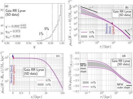
The posterior distribution of the DM density profile. Panel (a): the probability DF of the density flattening q. The three dashed vertical lines at q > 0.98 corresponds to (16, 50, 84) percentiles of the distribution. The lower 1 and 5 percentiles are located at q = 0.963 and 0.973, respectively. The posterior distribution rules out oblate dark halo models with q < 0.963 with a confidence level of |$99{{\ \rm per\ cent}}$|. We note that the parameter range at q > 1 is not explored in this paper. Panel (b): the density profile ρDM evaluated on the Galactic plane (R, z) = (r, 0). The shaded region corresponds to the central 68 per cent of the distribution, while the magenta solid lines denote the central 95 per cent of the distribution. The ranges of literature value of the local DM density ρDM(R0, 0) estimated from ‘local’ measurements and estimated from ‘global’ modelling of the Milky Way are shown by the blue and red vertical bands at R ≃ R0, respectively. (Literature data are taken from de Salas & Widmark 2020.) Panel (c): the same as panel (b), but for the density profile ρDM(R = R0, z) evaluated at the Solar cylinder as a function of the distance z from the Galactic plane. We note that the horizontal axis of this plot is linear at |$z\lt 1 \, \mathrm{kpc}$| and logarithmic at |$1 \, \mathrm{kpc}\lt z$|. Panel (d): the logarithmic density slope dln ρDM/dln r evaluated on the Galactic plane (R, z) = (r, 0).
Recently, Wegg et al. (2019) estimated the shape of the DM density profile by applying the axisymmetric form of the Jeans equations for the kinematic data for 15651 RR Lyrae stars at |$r\lt 20 \, \mathrm{kpc}$|. They also find that the shape of the DM halo is nearly spherical, with the density flattening of q = 1.00 ± 0.09, which is consistent with our result.
6.3.2 Dark matter density profile
Fig. 6(b) and (c) show the DM density profile evaluated at |$(R,z)=(R, 0 \, \mathrm{kpc})$| and at (R, z) = (R0, z), respectively. (We note |$R_0 = 8.178 \, \mathrm{kpc}$| is assumed; Gravity Collaboration 2019.) These profiles are sampled from the posterior distribution. We can see that our model puts a tight constraint on the radial and vertical density profiles. However, we need to be careful in interpreting this result. First, 99 per cent of the posterior distribution is distributed at 0.963 ≤ q ≤ 1, so the DM density profiles sampled from our posterior distribution are very close to spherical. Secondly, we use halo tracers that are distributed at |$5 \lesssim r/\, \mathrm{kpc}\lesssim 27.5$|. Thus, the inference of the DM density outside this range is less reliable. Third, the seemingly small variation in the density profile at large R and large |z| are probably because we fix the outer density slope of the DM to be ≃ (− 3) in the outer halo.
In spite of the above-mentioned complexities, we think our estimate of ρDM(R, 0) is reliable for |$1 \lesssim R/\, \mathrm{kpc}\lesssim 30$| based on our mock analysis in Appendix D. This can be understood in the following manner. Typical halo stars have very radially elongated orbits (β ≃ 0.8; see Fig. 5), indicating that they probably have relatively small pericentric radii. Therefore, many halo stars in our sample have orbits that are affected by the DM distribution in the inner few kpc and therefore their kinematics, even at large radii, reflect this information. To be specific, based on the best-fit DF model, we found that 20 per cent of the RR Lyrae stars in our sample have apocenter radius larger than |$r = 29.7 \, \mathrm{kpc}$| and that 20 per cent of the stars have pericenter radius smaller than |$r = 0.4 \, \mathrm{kpc}$|. For our mock analysis with smooth-halo mock data (Appendix D1), within |$0.4 \lt r/\, \mathrm{kpc}\lt 29.7$|, we can constrain the DM density with less than 30 per cent uncertainty. This result supports the idea that we can constraint the DM profile outside |$5 \lt r/\, \mathrm{kpc}\lt 27.5$|.
6.3.3 Dark matter density slope
In our analysis, the inner density slope (−γ) of the DM halo is a free parameter, while the outer density slope is fixed to be (−3). The central 68 per cent of the posterior distribution of γ is distributed at 0.785 < γ < 1.209 (see Table 2), which is consistent with a cusped NFW profile with γ = 1 (Navarro et al. 1997). Fig. 6(d) shows the DM logarithmic density slope dln ρDM/dln r as a function of Galactocentric radius r evaluated at (R, z) = (r, 0). As we can see from this figure, the logarithmic density slope is approximately (−1) at |$r \simeq 1 \, \mathrm{kpc}$|.
6.3.4 Other constraints on the dark matter distribution
Table 2 summarizes the key properties of the DM density profile derived from our analysis. For example, our result constraints the local DM density to, |$\rho _{\mathrm{DM},\odot } = (9.01^{+0.18}_{-0.20})\times 10^{-3}{\,\rm M_\odot} \, \mathrm{pc}^{-3}$|, which is equivalent to |$0.342^{+0.007}_{-0.007}$| GeVcm−3. The quoted uncertainty in ρDM,⊙ in our analysis only takes into account the random error. We note that de Salas et al. (2019) pointed out that the use of different functional forms of the baryonic potential could cause systematic shifts in ρDM,⊙. For reference, de Salas et al. (2019) assumed a generalized-NFW model for the DM density profile, and estimated |$\rho _{\mathrm{DM},\odot } = 7.89^{+0.74}_{-0.71}\times 10^{-3}{\,\rm M_\odot} \, \mathrm{pc}^{-3}$| and |$10.18^{+0.89}_{-0.95}\times 10^{-3}{\,\rm M_\odot} \, \mathrm{pc}^{-3}$| for their baryonic model B1 and B2, respectively. Apart from the systematic error due to the choice of our baryonic mass model, our measurement is slightly smaller than previous measurements of ρDM,⊙ = (11–|$16)\times 10^{-3} {\,\rm M_\odot} \, \mathrm{pc}^{-3}$| derived from analyses of Solar-neighbour stars (Bienaymé et al. 2014; McKee, Parravano & Hollenbach 2015; de Salas & Widmark 2020), while it is consistent with previous measurements of ρDM,⊙ = (8–|$13)\times 10^{-3} {\,\rm M_\odot} \, \mathrm{pc}^{-3}$| derived from analyses of global modelling of the Milky Way such as rotation curve (Piffl et al. 2014; de Salas et al. 2019; Cautun et al. 2020; de Salas & Widmark 2020). For the various measurements of ρDM,⊙ before and after the advent of Gaia data, we refer readers to reviews by Read (2014) and de Salas & Widmark (2020), respectively.
We also derive the enclosed mass of the DM and the enclosed mass of the DM plus baryons at various radii r. For example, our result indicates that the DM mass within the virial radius r200 is |$M_{200} = 0.730^{+0.046}_{-0.052} \times 10^{12} {\rm {\,\rm M_\odot}}$|, which is consistent with some recent studies (see Wang et al. 2020 for a review), but slightly lower than (0.90 ± 0.13) × 1012 M⊙ recently found by Vasiliev et al. (2021). However, we note that this result may be dominated by our prior on Mstar/M200, since our sample is distributed in the inner part of the halo at |$5 \lesssim r/\, \mathrm{kpc}\lesssim 27.5$|.
7 DISCUSSION
7.1 Comparison with other studies
We have analysed the kinematics of RR Lyrae stars to estimate the DM density distribution, especially focusing on the flattening q of the DM halo within 30 kpc. Our result indicates that q > 0.963 with 99 per cent confidence level, which is consistent with a nearly spherical DM halo, although we cannot currently explore the possibility that q > 1 (prolate). Here, we compare our result with previous studies.
7.1.1 Previous results with stellar streams
Koposov et al. (2010) modelled GD-1 stellar stream (Grillmair & Dionatos 2006) and estimated the flattening of the Galactic potential. They found that the DM potential’s flattening is qΦ > 0.89 with 90 per cent confidence level. According to a relationship between the density flattening and the potential flattening,10 their constraint corresponds to a density flattening of q > 0.68 with 90 per cent confidence level. Bovy et al. (2016) measured the DM density flattening to be |$q=1.3^{+0.5}_{-0.3}$| when using GD-1 stream (at |$r=14 \, \mathrm{kpc}$|) and q = 0.93 ± 0.16 when using Pal 5 stream (at |$r=19 \, \mathrm{kpc}$|). By combining these two data sets, they estimated the global value of q to be q = 1.05 ± 0.14. More recently, Malhan & Ibata (2019) analysed the GD-1 stream by using the astrometric data from Gaia DR2 to estimate |$q = 0.82^{+0.25}_{-0.13}$|. Although the statistical uncertainties are relatively large, all of the above-mentioned results using the GD-1 stream are consistent with a nearly spherical DM halo.
Law & Majewski (2010) modelled the Sagittarius stellar stream to conclude that the best-fitting Galactic DM halo model is oblate-triaxial with the major axis lying in the Galactic disc plane about 7○ to the Galactocentric y-axis, the intermediate axis perpendicular to the stellar disc, and the short axis lying 7○ from the Galactic x-axis. The DM density distribution is flattened such that the axis lengths of the density distribution along Galactocentric x, y, z are given by x: y: z = 0.44: 1: 0.97. This model of the halo is strongly disfavoured since simulations show that stellar discs perpendicular to the intermediate axis of such a halo are violently unstable (Debattista et al. 2013). In addition, Pearson et al. (2015) argued that the triaxial potential model by Law & Majewski (2010) is not a good approximation at least at |$r\lt 20 \, \mathrm{kpc}$| since it would cause too much dispersal and thickening to the Pal 5 stellar stream.
Recently Vasiliev et al. (2021) constructed a halo model that fits Gaia DR2 proper motion data as well as all available radial velocity data with a time-dependent Galactic halo model that includes the reflex motion resulting from the gravitational perturbation by the Large Magellanic Cloud (LMC). These authors find that the models that fit the Sagittarius stream best, include deformation to the MW DM distribution such that the halo is oblate with an axial ratio R: z ≃ 1: 0.6 and aligned with the disc in the inner part of the halo, but becoming triaxial (twisted and then prolate-triaxial) and misaligned with the disc beyond |${\sim}50 \, \mathrm{kpc}$|.
7.1.2 Previous results with field halo tracers
Loebman et al. (2014) applied the axisymmetric Jeans equations to kinematic data for field halo stars from SDSS and estimated the DM halo’s density flattening to be q ≃ 0.4 ± 0.1. This estimate is significantly smaller than most other studies (except for the recent work based on the Sagittarius stream when influenced by the LMC; Vasiliev et al. 2021). Interestingly, they also found that their halo sample has a radial velocity dispersion |$\sigma _r \simeq 141 \, \mathrm{km\ s}^{-1}$| across the survey volume (|$d \lesssim 10 \, \mathrm{kpc}$|), while we find |$\sigma _r \simeq 180 \, \mathrm{km\ s}^{-1}$| near the Sun dropping to |$\sigma _r \simeq 160 \, \mathrm{km\ s}^{-1}$| at R ∼ 20 kpc. If our RR Lyrae sample and their halo sample trace the same population of halo stars, this disagreement might arise from two sources. First Loebman et al. (2014) used a proper motion sample derived from SDSS and POSS which has significantly larger errors than Gaia DR2 proper motions. Second, they used photometric distances to their field star sample which are less accurate than distances to the Gaia RRLyrae sample.
Wegg et al. (2019) applied a similar axisymmetric Jeans equation formalism to an RR Lyrae sample from Gaia DR2 and estimated the DM density flattening to be q ≃ 1.00 ± 0.09. Their sample overlaps significantly with our RR Lyrae sample, and their spatial selection cut is similar to ours. The fact that our result is also consistent with a spherical DM halo provides strong evidence that the DM halo within r < 30 kpc is not highly oblate (however see Section 7.2.1 and Appendix D2 for the effects of disequilibrium).
It is worth mentioning that Posti & Helmi (2019) modelled the kinematics of globular clusters with an action-based DF model and estimated q = 1.3 ± 0.25 (prolate). They used AGAMA to compute the orbital actions. However, the method to compute actions that is implemented in AGAMA is inapplicable to prolate potentials, but the package does not explicitly forbid their use (see Section 3.1.5 for more details on this point). In this regard, the validity of their analysis is questionable.
7.1.3 Prediction from numerical simulations
As mentioned in Section 1, numerous cosmological hydrodynamical simulations over the past 15 years have predicted that the DM halo of MW-sized galaxies have oblate axisymmetric shapes within the inner (0.15–0.3)r200. The most recent value of the mean flattening based on several thousand galaxies from the Illustris simulations being 〈q〉 = 0.79 ± 0.15 (Chua et al. 2019) within ∼0.15r200 ∼ 30 kpc. This is much flatter than the q value obtained from our analysis, which excludes an oblate halo with q < 0.963 with a confidence level of 99 per cent. This could either imply a tension between the predictions of cosmological hydrodynamical simulations and our results or it could imply that some of our assumptions, principally, the assumption of dynamical equilibrium (as discussed in Section 7.2.1 and Appendix D2), could be in doubt. Additional applications of this method to mock data from cosmological simulations and haloes that are out of equilibrium, e.g. due to the interaction with the LMC, are in progress to quantify the effects of disequilibrium and to better assess the source of this disagreement (de Salas et al., in preparation).
7.2 Some issues in our analysis
7.2.1 Dynamical disequilibrium
We have assumed that the MW is in dynamical equilibrium. However, this assumption might be too simplistic. For example, Iorio & Belokurov (2019) pointed out that the RR Lyrae sample used here shows a triaxial spatial distribution within r < 30 kpc that has its principal axes tilted relative to the principal axes of the Galactic potential, and is possibly misaligned with the Galactic disc. This triaxial distribution of RR Lyrae stars in the inner stellar halo is thought to have been deposited by a highly radial accretion event referred to as the ‘Gaia–Sausage’ (Belokurov et al. 2018) or ‘Gaia–Enceladus’ (Helmi et al. 2018). Additional evidence for disequilibrium comes from the observation of two prominent substructures in the RRLyrae sample, the Hercules–Aquila Cloud and the Virgo Overdensity (Simion, Belokurov & Koposov 2019), which might be related to the same accretion event (cf. Naidu et al. 2021).
In this regard, it is worth mentioning that we also applied our code to a mock data set generated from one galaxy m12m from the Fire-2 Latte cosmological hydrodynamical suite of simulations (Wetzel et al. 2016; Hopkins et al. 2018; Sanderson et al. 2020). Like the real MW, this galaxy is not in perfect dynamical equilibrium and includes halo substructure. Our modelling of this galaxy results in an overestimate of the value of q (see Fig. D7). This is in contrast with our analysis with mock data sets generated from smooth, equilibrium halo models, which successfully recovers the input values of q with no obvious systematic bias (see Fig. D3). Thus, if the RR Lyrae stars in the inner halo used in our analysis and Wegg et al. (2019) are significantly out of equilibrium, the assumption of dynamical equilibrium could have resulted in an overestimate of q. While analyses of several more similar cosmological simulations are needed to assess how much of an overestimate can be expected from disequilibrium our analysis of galaxy m12m suggests an inflation of Δq ∼ 0.1−0.2 implying that the true flattening could be closer to q ∼ 0.75−0.90.
Erkal, Belokurov & Parkin (2020) argued that the perturbation from LMC is not negligible at |$r \gtrsim 30 \, \mathrm{kpc}$|. If the LMC’s perturbation is strong, our DF fitting method might result in a biased estimate of q (see also Petersen & Peñarrubia 2021). However, the inner part of the halo is less affected by such a perturbation (Garavito-Camargo et al. 2020), so our analysis may not be seriously affected by LMC’s perturbation. Recently, Vasiliev et al. (2021) modelled the dynamics of the MW, LMC, and the Sagittarius dwarf galaxy. They also estimated the radial profile of the DM halo’s shape based on the morphology of the Sagittarius stream. In principle, it is possible to formulate how LMC affects the DF, but this is beyond the scope of this paper (see Deason et al. 2021).
7.2.2 More general shapes for the dark matter halo
Throughout this paper, we have assumed that q is constant as a function of radius. However, if q changes as a function of r, as predicted by cosmological hydrodynamical simulations (e.g. Zemp et al. 2012) our estimate of q might be biased. In principle, we can relax the assumption of constant q with some extra parameters, such as the inner and outer values of q and the transition radius.
We also note that, it is possible to estimate the triaxiality of the DM halo by implementing a fast algorithm to compute actions in a general triaxial potentials (including prolate potentials, with long axis oriented perpendicular to the disc plane), such as the method of Sanders & Binney (2015a). The fact that our posterior distribution of q is peaked at q = 1, the upper boundary of the currently explored range of q, points to the need for future investigations of prolate and triaxial halo shapes.
7.2.3 Metallicity dependence of the distribution function
There is some observational evidence that the DF of the stellar halo depends on the metallicity (Carollo et al. 2007, 2010; Deason et al. 2011; Hattori et al. 2013; Kafle et al. 2013; Das & Binney 2016; Bird et al. 2019; Carollo & Chiba 2021; Iorio & Belokurov 2021). In this paper, we do not take into account the metallicity dependence, because it would increase the number of free parameters. Our sample is confined to the inner halo (r ≲ 27.5), where relatively metal-rich halo stars ([Fe/H]>−2) dominate, therefore the DF is probably most representative of metal-rich stars. However, if we were to apply our method to a sample of stars in a larger volume (say |$r \lesssim 100 \, \mathrm{kpc}$|), the metallicity dependence would be more important.
7.3 Other studies of distribution function fitting
As mentioned in Section 1, there have been several previous efforts to use the DF to construct models of the MW (both global models and models of individual components). We briefly summarize some of these other DF-based studies to put our work in the context.
McMillan & Binney (2012), McMillan & Binney (2013) formulated a Bayesian way of estimating the parameters of the DF of the stellar disc when the MW potential is given. In these works, they introduced some important ideas regarding DF fitting, such as (i) an efficient algorithm to compute the relative likelihood of the model given observational data with or without missing data; and (ii) the effect of the observational selection function. They used mock data sets of disc stars to show that the MW potential can be reliably measured with the DF fitting method. In our paper, we have followed the formulation by McMillan & Binney (2013).
In both McMillan & Binney (2012) and McMillan & Binney (2013), the distance uncertainty was not properly taken into account in evaluating the normalization factor of the DF. The effect of the distance uncertainty in the normalization was first rigorously formulated by Trick et al. (2016), although they did not use their rigorous formulation for their mock analysis. Instead, they used a simplified formulation that is equivalent to the formulation by McMillan & Binney (2013). Yet, they showed that the DF fitting can be used to estimate the MW potential within |${\sim}4 \, \mathrm{kpc}$| from the Sun with a reasonable size of mock data set. Our work adopted the formalism of Trick et al. (2016) and introduced a practical way of computing the normalization factor rigorously for the first time.
Using simple mock data sets with no observational errors, Ting et al. (2013) demonstrated that simultaneous fitting of the stellar disc DF and the MW potential can reconstruct the input model accurately. Bovy & Rix (2013) applied this methodology to 16269 disc stars in SDSS/SEGUE. They divided the sample into mono-abundance populations (MAPs) with similar chemistry ([Fe/H] and [α/Fe]). For each MAP, they simultaneously fit the parameters of the DF and the MW potential, which they used to estimate the vertical force Kz at |$z=1.1 \, \mathrm{kpc}$| at a representative R that is determined by the spatial distribution of the MAP. They further used the profile of the |$K_z(R, z=1.1 \, \mathrm{kpc})$| and an additional data set of the terminal velocity to estimate the MW potential. Their DF-based modelling approach in the first half of Bovy & Rix (2013) is close to ours, and their analysis of vcirc data and Kz data in the second half of Bovy & Rix (2013) corresponds to our additional analysis in Appendix C.
Similar analyses were also done for more extended sample of stars that include both halo and disc stars. Piffl et al. (2014) used ∼200000 giants from RAVE survey to find the maximum-likelihood model of the MW. They introduced a composite DF model consisting of a disc-like DF and a halo-like DF, although their sample is dominated by the disc stars. Binney & Piffl (2015) and Cole & Binney (2017) extended the work of Piffl et al. (2014) and modelled both the stellar disc and the dark halo with action-based DF models that self-consistently generated gravitational potential. Most importantly, Binney & Piffl (2015) and Cole & Binney (2017) did not directly model the density profile of the DM halo, but they modelled the DF of the DM halo instead. One advantage of using the DF of the DM is that they can handle the deformation of the DM halo by the baryonic distribution, as discussed in Piffl, Penoyre & Binney (2015).
Although the above-mentioned studies fit both the DF and the MW potential, there have been some studies in which the MW potential was fixed and the DFs of the tracers were investigated. Sanders & Binney (2015b) used the position-velocity data and [Fe/H] data for nearby disc stars from Geneva-Copenhagen Survey and SEGUE survey and analysed the structure of the MW disc with an action-based DF. Das & Binney (2016) and Das et al. (2016) used K giants and blue horizontal branch stars from SEGUE survey to analyse the MW stellar halo with an action-based DF. Binney & Wong (2017) analysed the position-velocity data for 157 globular clusters in the MW, by using an action-based DF model consisting of a disc-like rotating DF and a halo-like non-rotating DF.
8 CONCLUSIONS
In this paper, we have combined proper-motion data from Gaia DR2 for halo RR Lyrae stars within |$d \le 20 \, \mathrm{kpc}$| from the Sun (Iorio & Belokurov 2019), circular velocity data for red giants in the disc plane from Gaia DR2 (Eilers et al. 2019), and the vertical force data from SDSS/SEGUE (Bovy & Rix 2013) to constrain the 3D shape of the Galactic DM halo, by assuming that the stellar halo can be described by an analytic DF model and that the MW is oblate-axisymmetric.
Our method is based on the DF fitting formulation that was pioneered by McMillan & Binney (2012), McMillan & Binney (2013), and elaborated upon by Ting et al. (2013) and Trick et al. (2016). Our most important contribution to the DF fitting formalism is the introduction of a new way to handle the distance uncertainty of sample stars.
The main results of our modelling of the MW halo can be summarized as follows:
In total, 99 per cent of the posterior distribution of q = c/a (minor-to-major axial ratio of the DM density) is located at q > 0.963 (see Fig. 6a). We emphasize that we only explored oblate models with q ≤ 1 due to the limitations in the way we compute orbital actions of halo stars.
Our estimated value of q > 0.963 implies a nearly spherical DM halo within |$r \lesssim 30 \, \mathrm{kpc}$| and strongly disfavours a very flattened DM halo. This may be in conflict with recent ΛCDM cosmological simulations that predict 〈q〉 = 0.79 ± 0.15 (Chua et al. 2019) within |$0.15r_{200} ({\sim}30 \, \mathrm{kpc})$|.
While validation tests of our code with with mock data created from smooth, equilibrium galactic models recover the values of q to high accuracy (see Fig. D3), our test with mock data generated from a galaxy (m12m) from the Fire-2 Latte cosmological hydrodynamical suite of simulations yields q values overestimated by ∼0.1−0.2 (see Fig. D7). This implies that if the MW halo is not in dynamical equilibrium as we have assumed, our estimate of q is an overestimate.
Our derived DF is a good match to the proper motion distribution in (l, b) and the derived correlation coefficient |$\rho _{\mu _{\ell *}\mu _{b}}$| accurately models, for the first time, the quadrupole feature characteristic of the radially anisotropic distribution observed in the data (see Fig. 4). The derived DF also provides an estimate of the radial, azimuthal and polar velocity dispersion profiles (σr(r), σϕ(r), σθ(r)) and velocity anisotropy β(r) that are a good match to observed velocity dispersion and anisotropy profiles of K giant stars (Bird et al. 2019), which were not used in our analysis (see Fig. 5).
Our result puts a tight constraint on the local DM density: ρDM,⊙ = |$0.00901^{+0.00018}_{-0.00020} {\,\rm M_\odot} \, \mathrm{pc}^{-3}$|, or |$0.342^{+0.007}_{-0.007}$| GeVcm−3 (see Fig. 6c and Table 2), which is consistent with other recent estimates (e.g. see reviews by Read 2014; Bland-Hawthorn & Gerhard 2016; de Salas & Widmark 2020).
Our result favours a cuspy DM halo with inner density slope |$(-\gamma) = -\left(0.982^{+0.227}_{-0.197} \right)$|, which is consistent with an NFW profile (see Fig. 6b–d and Table 2).
ACKNOWLEDGEMENTS
The authors thank the referee for thorough reading and constructive comments that improved the manuscript. KH thanks Giuliano Iorio for kindly sharing the clean sample of RR Lyrae stars in Iorio & Belokurov (2019), and Robyn Sanderson and Andrew Wetzel for kindly sharing the Latte simulations. KH thanks Sergey Koposov for useful conversations and for his support. KH thanks Pablo F. de Salas for frequent discussions that improved KH’s analysis code. KH thanks AH for the support during this work. KH is supported by JSPS KAKENHI Grant Numbers JP21K13965 and JP21H00053. KH and MV thank members of the stellar haloes group at the University of Michigan for continued camaraderie and stimulating discussion. MV and KH were supported by NASA-ATP award NNX15AK79G. MV is also supported by NASA-ATP award 80NSSC20K0509. This work was supported by a Michigan Institute for Computational Discovery and Engineering (MICDE) catalyst grant for FY2019. EV acknowledges support from STFC via the Consolidated grant to the Institute of Astronomy. Some part of this research was started at the KITP workshop ‘Dynamical Models for Stars and Gas in Galaxies in the Gaia Era’ held at the Kavli Institute for Theoretical Physics. This work has made use of data from the European Space Agency (ESA) mission Gaia (http://www.cosmos.esa.int/gaia), processed by the Gaia Data Processing and Analysis Consortium (DPAC, http://www.cosmos.esa.int/web/gaia/dpac/consortium). Funding for the DPAC has been provided by national institutions, in particular the institutions participating in the Gaia Multilateral Agreement.
We used the following packages: AGAMA (Vasiliev 2019), constrNMPy (https://github.com/alexblaessle/constrNMPy), corner.py (Foreman-Mackey 2016), cubature (https://github.com/stevengj/cubature), emcee (Foreman-Mackey et al. 2013), gizmo_read (https://bitbucket.org/awetzel/gizmo_read), matplotlib (Hunter 2007), numpy (van der Walt, Colbert & Varoquaux 2011), PyGaia (https://github.com/agabrown/PyGaia), and scipy (Jones, Oliphant & Peterson 2001).
DATA AVAILABILITY
The MCMC chains obtained from our analysis are available upon reasonable request.
Footnotes
While other methods to measure the DM halo’s shape have been proposed, they have not been used very extensively. For example, Olling & Merrifield (2000) used the flaring of the HI gas disc to determine the flattening of the DM halo, and Gnedin et al. (2005) proposed the use of proper motions of hypervelocity stars to derive the triaxiality of the halo.
Since the fraction of excluded stars is negligible, it is safe to regard our sample as a kinematically unbiased sample.
In the case of self-consistent DF model (which is not the case for our application), there is a relationship such that the density behaves as ρ ∝ r−γ with γ = (4Γ − 6)/(Γ − 1) in the inner region and behaves as ρ ∝ r−β with β = (B + 3)/2 in the outer region.
In Appendix D, we fix κ = 0 and set Jϕ,0 = constant for our analysis with mock data created from smooth halo models. In contrast, we treat (κ, Jϕ,0) as free parameters when we analyse the mock data created from one of the cosmological hydrodynamical simulations (m12m), since the stellar halo shows a net rotation.
For example, even if (N − 1) stars perfectly follow an action-based model M, an addition of a single unbound star would make the total likelihood of the model M zero. This is because action |$\rm{\boldsymbol {J}}$| is not defined for an unbound star and therefore |$f(\rm{\boldsymbol {x}}, \rm{\boldsymbol {v}})=0$| for the unbound star if f is action-based.
However, we note that the Jacobian factor is missing in equations 15–16 (in their section 2.7) of Trick et al. (2016).
The reason for using a Cauchy distribution is related to this weight. If we were to use a Gaussian distribution or any thin-tailed distribution, this weight would become very large for a Monte Carlo sample with large |$|{v_{\mathrm{los}}^{\prime }}_{ij} - (- \rm{\boldsymbol {v}}_\odot \cdot \rm{\boldsymbol {e}}_{\mathrm{los},i})|$|. This means that a small number of such Monte Carlo samples may dominate the integral, causing a large systematic error in the Monte Carlo integration. This problem is minimized if we use a fat-tailed distribution such as Cauchy distribution. Note that the above-mentioned problem could be minimized if we could use a large enough number of Monte Carlo points NMC, which is impractical in our case due to the computational cost.
If we are to run MCMC for 5000 steps (with a single MCMC ‘walker’), we need to evaluate the likelihood 5000 times. This would take ∼1 month assuming 10 min per model for evaluating likelihood.
We note that these quantities are derived from the covariance matrix of the proper motion distribution along each line of sight, which is different from the covariance matrix of the observational error for each star Σμ used in equation (22).
For a potential model with a nearly flat rotation curve, the density flattening q and the potential flattening |$q_\Phi$| are related by |$q^2 \simeq 2 q_\Phi ^4 - q_\Phi ^2$| (see equation 2.72b of Binney & Tremaine 2008).
Bovy & Rix (2013) derived the vertical force at |$|z|=1.1 \, \mathrm{kpc}$| by analysing the kinematics of disc stars with an assumption that the Galactic DM halo is spherical. Thus, one might worry whether using Bovy & Rix (2013)’s vertical force data introduces a bias such that the posterior distribution of q prefers a spherical DM halo. The additional analysis presented here shows that we do not need to worry about this potential source of bias.
We assume that RR Lyrae stars have a colour (V − I) = 0.6 and V-band absolute magnitude MV = 0.6 (e.g. Yepez et al. 2018). We derive (G − V) and MG = MV + (G − V) with PyGaia (https://github.com/agabrown/PyGaia).
Table 2 of Sanderson et al. (2020) suggests that m12m’s stellar disc has a scale radius of |${\sim}3.2 \, \mathrm{kpc}$| when they fit the stellar disc at |$|z|\lt 0.3 \, \mathrm{kpc}$| and |$6 \, \mathrm{kpc}\lt R\lt 12 \, \mathrm{kpc}$| with a single exponential disc model. The same table also suggests that 90 percent of the disc stars are located at |$|z| \lt 2.3 \, \mathrm{kpc}$|. If we assume a single-component stellar disc with a constant scale height of zd, this result means that |$1-\exp (-2.3 \, \mathrm{kpc}/ z_\mathrm{d}) = 0.9$|, or |$z_\mathrm{d} \simeq 1 \, \mathrm{kpc}$|. These scale radius and scale height are consistent with those of our ‘component 2’, which is the dominant component at |$|z|\lt 0.3 \, \mathrm{kpc}$| and |$6 \, \mathrm{kpc}\lt R\lt 12 \, \mathrm{kpc}$|.
REFERENCES
APPENDIX A: COORDINATE SYSTEM
We adopt a right-hand Galactocentric Cartesian coordinate system (x, y, z), in which the (x, y)-plane is the Galactic disc plane. The x-axis is directed from the Sun to the Galactic centre, the y-axis is parallel to the direction of the Galactic rotation at the Solar position (i.e. the direction of ℓ = 90○ as seen from the Sun), and the z-axis is perpendicular to the Galactic disc. The position of the Sun is assumed to be |$\rm{\boldsymbol {x}}_\odot = (x_\odot ,y_\odot ,z_\odot) = (-R_0,0,0)$|, with |$R_0 = 8.178 \, \mathrm{kpc}$| (Gravity Collaboration 2019). The velocity of the Sun with respect to the Galactic rest frame is assumed to be |$\rm{\boldsymbol {v}}_\odot = (v_{x,\odot },v_{y,\odot },v_{z,\odot }) = (11.10, 247.30, 7.25) \, \mathrm{km\ s}^{-1}$| (Reid & Brunthaler 2004; Schönrich, Binney & Dehnen 2010). We also define a Galactocentric spherical coordinate system (r, ϕ, θ) and a Galactocentric cylindrical coordinate system (R, ϕ, z), such that (x, y, z) = (rcos θcos ϕ, rcos θsin ϕ, rsin θ) = (Rcos ϕ, Rsin ϕ, z). Also, for each 3D location with respect to the Sun, we define the line-of-sight unit vector |$\rm{\boldsymbol {e}}_\mathrm{los}$|.
APPENDIX B: FULL RESULT OF OUR MCMC ANALYSIS
Figs B1 and B2 show corner plots of the posterior distributions resulting from our fiducial analysis. The quantities shown in Fig. B1 are the raw variables used in our MCMC, while the quantities shown in Fig. B2 are more physically meaningful quantities.
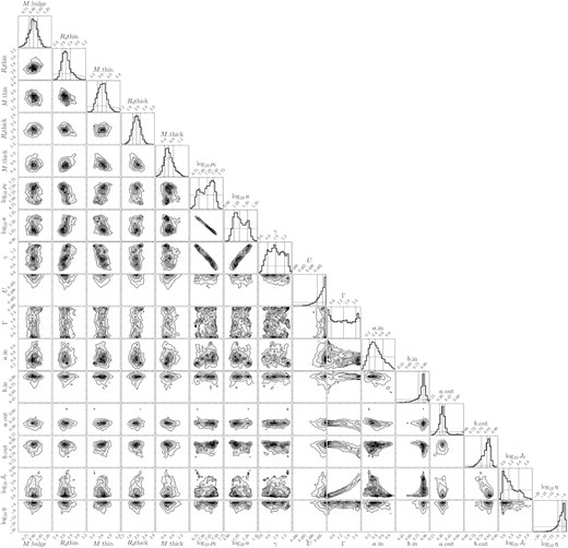
The corner plot of all the parameters in our analysis of Gaia RR Lyrae stars. The parameters shown here are the parameters for the baryonic mass distribution (Mbulge/(1010 M⊙), |$R_\mathrm{d}^\mathrm{thin}$|, Mthin/(1010M⊙), |$R_\mathrm{d}^\mathrm{thick}$|, Mthick/(1010M⊙)), the parameters for the DM mass distribution (log10ρ0, log10a, γ, U), and the parameters for the DF (Γ, ain, bin, aout, bout, log10J0, log10η). The top panel of each column shows the the posterior distribution of each parameter (thick solid histograms), and the corresponding prior distribution (thin-dashed histograms).
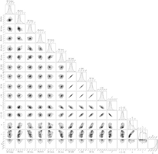
The same as Fig. B1, but expressed by more physically meaningful quantities. The parameters shown here are the parameters for the baryonic mass distribution (Mbulge/(1010 M⊙), |$R_\mathrm{d}^\mathrm{thin}$|, Mthin/(1010 M⊙), |$R_\mathrm{d}^\mathrm{thick}$|, Mthick/(1010 M⊙), Mstar/(1010 M⊙)) and the parameters for the DM mass distribution (M200/(1012 M⊙), r200, M94/(1012M⊙), r94, c′, r−2, a, γ, q).
In Fig. B1, the top panel of each column, also shows the prior distribution for each parameter (dashed blue histrograms). By comparing the posterior (solid black histograms) and prior distributions, we can see that the bulge and thick-disc parameters are essentially determined by the prior distributions, while the thin-disc and DM-halo parameters are constrained by the data.
APPENDIX C: COMPARISON WITH A POTENTIAL-ONLY FIT
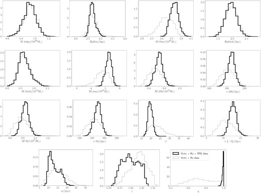
The posterior distribution of our analyses with and without using RR Lyrae data. The solid black histograms show the posterior distributions from our fiducial analysis, in which we used all three kinds of data. The dotted green histograms show the posterior distributions for a test in which we used the circular velocity data and vertical force data only (see Appendix C for details). The parameters shown here are the same as in Fig. B2. We see that the DM’s flattening parameter q can be well constrained if we use the RR Lyrae data in our inference. We note that the area below each histogram is normalized to unity, except for the green dotted histogram for q, which is multiplied by 100 for greater visibility.
On the one hand, the posterior distributions of parameters (a, γ, c′, q) and quantities characterizing the DM halo (e.g. virial mass and virial radius) are improved (become narrower) by using the RR Lyrae data. This improvement is most significant for the density flattening q of the DM halo. As we can see from the bottom right-hand panel, q is poorly constrained when we use the circular velocity data and the vertical force data only. In contrast, when we also use the RR Lyrae data, the posterior distribution of q is highly peaked. Based on this additional analysis, we can conclude that the posterior distribution of q in our fiducial analysis is peaked near q = 1 primarily because of the kinematic data of RR Lyrae stars, and not because of the circular velocity data or the vertical force data. This result is reassuring, because our main motivation in this paper is to constrain q by using halo tracers.11
On the other hand, many parameters for the baryonic components, such as the bulge or the thick disc, show no significant improvement when we additionally use the RR Lyrae data. (The only exception is the mass of the thin disc Mthin, whose posterior distribution is peaked at higher value when RR Lyrae data are additionally used. As a result, the total stellar mass Mstar = Mbulge + Mthin + Mthick is also peaked at higher value.) This result indicates that many baryonic parameters are almost exclusively determined by the circular velocity data, the vertical force data, and our prior distribution. Intriguingly, de Salas et al. (2019) also found that their posterior distribution for the parameters of the baryonic model is dominated by their prior when they analysed the same vcirc data. Our result confirms the result of de Salas et al. (2019) even in the presence of additional data such as Kz data or the kinematic data of halo stars. This result indicates that precise knowledge of the baryonic potential is essential for our understanding of the Galactic DM distribution.
APPENDIX D: VALIDATION OF OUR METHOD WITH MOCK DATA
To validate our method and results for the Gaia RR Lyrae sample, we perform similar analyses with eight mock data sets summarized in Table D1. For each of the models below, we generate a 5D mock data set without vlos and a 6D mock data set. The number of mock stars and the survey selection function are identical to those for the RR Lyrae sample.
Summary of mock data used for validation and results.
| Base model | True DM density flattening | Data type | ρDM(R, 0, 0) | ρDM(R0, 0, z) | q |
|---|---|---|---|---|---|
| Analytic DF model + analytic potential model | qtrue = 0.6 | 5D | Fig. D1(a) | Fig. D2(a) | Fig. D3(a) |
| Analytic DF model + analytic potential model | qtrue = 0.8 | 5D | Fig. D1(b) | Fig. D2(b) | Fig. D3(b) |
| Analytic DF model + analytic potential model | qtrue = 0.996 | 5D | Fig. D1(c) | Fig. D2(c) | Fig. D3(c) |
| Analytic DF model + analytic potential model | qtrue = 0.6 | 6D | Fig. D1(d) | Fig. D2(d) | Fig. D3(d) |
| Analytic DF model + analytic potential model | qtrue = 0.8 | 6D | Fig. D1(e) | Fig. D2(e) | Fig. D3(e) |
| Analytic DF model + analytic potential model | qtrue = 0.996 | 6D | Fig. D1(f) | Fig. D2(f) | Fig. D3(f) |
| m12m galaxy | Fig. D4 | 5D | Fig. D5(a) | Fig. D6(a) | Fig. D7(a) |
| m12m galaxy | Fig. D4 | 6D | Fig. D5(b) | Fig. D6(b) | Fig. D7(b) |
To generate these mock data, we prepare three smooth stellar halo models constructed from analytic DFs embedded in analytic potential models, as detailed in Appendix D1.1. We also generated a mock date set from a realistic Milky-Way-like galaxy m12m from the Fire-2, Latte cosmological hydrodynamical simulation suite (Wetzel et al. 2016; Hopkins et al. 2018; Sanderson et al. 2020), as detailed in Appendix D2.4.
D1 Validation with ‘smooth halo’ mock data sets
D1.1 Mock data for smooth stellar halo models
We construct three smooth stellar halo models. We assume that the halo stars are test particles moving in an analytic potential composed of baryonic component and DM component. The functional form of the model potential (bulge, thin/thick/gas discs and DM halo) and the functional form of the stellar halo DF are identical to those in Section 3. We adopt the same gas disc model as in McMillan (2017), and we adopt three sets of parameters for bulge, thin disc, thick disc, DM halo, and stellar halo DF model:
the best-fitting parameters shown in Table 1 (with q = 0.996);
the same as the best-fitting parameters but with q = 0.8; and
the same as the best-fitting parameters but with q = 0.6.
In other words, these models are different from each other only in terms of the DM density flattening q.
For each model, we evaluate the circular velocity |$v_\mathrm{circ}^\mathrm{model}(R)$| at the same radii as in the data of Eilers et al. (2019) and take into account the same amount of observational error. Also, for each model, we evaluate the vertical force |$K_{z,1.1 \, \mathrm{kpc}}^\mathrm{model}(R)$| at the same locations as in the data of Bovy & Rix (2013) and take into account the same amount of fractional error. The mock data of circular velocity and vertical force are used to aid our DF fitting.
To generate mock RR Lyrae stars, we first sample mock halo stars from the above-mentioned three input models. We then add Gaia DR2-like proper motion errors that depend on the Gaia’s G-band photometry. For this purpose, we assume that all the mock stars are RR Lyrae stars with G-band absolute magnitude12MG = −0.1376, and compute Gaia DR2-like proper motion error by using a formula described in equation (16) in Sanderson et al. (2020). We also add a distance modulus uncertainty of 0.240 (mimicking RR Lyrae stars), and an optimistic |$5 \, \mathrm{km\ s}^{-1}$| error on vlos.
From this sample of error-added mock stars, we randomly choose N = 16197 stars by using the spatial selection function defined in Section 3.3. In the following, we use three sets of ‘6D mock data’ and three sets of ‘5D mock data’ for which we mask vlos.
D1.2 Radial dark matter density
Fig. D1 shows the reconstructed DM density |$\rho _\mathrm{DM}(R, z=0 \, \mathrm{kpc})$|. We see that the central 68 percentile region (grey shaded region) traces the true DM profile (dashed line) for all mock data.
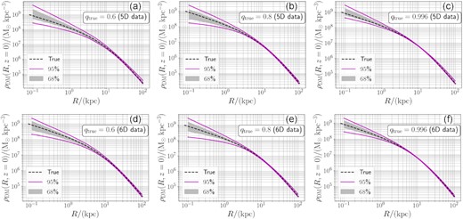
The DM density profile |$\rho (R,z=0 \, \mathrm{kpc})$| reconstructed from our mock analysis. The input value of the flattening, qtrue, is shown in each panel. The shaded region and the region enclosed by solid lines cover the central 68 and 95 percentiles of the posterior distribution. Also, the dashed line corresponds to the true profile of the input model. In panels (a)–(c), the results are shown for DF fitting with 5D data (without vlos data). In panels (d)–(f), the results are shown for DF fitting with 6D data. The agreement between the true profile and the posterior profile indicates that our method can recover the DM profile even if we lack the vlos data.
Although the spatial distribution of our mock sample stars is limited by the survey volume, the inferred density profile traces the actual density profile even beyond the survey volume. Given that the inner density slope is allowed to vary freely, it is intriguing that the DF fitting can recover well the radial DM density profile at |$1\lt R/\, \mathrm{kpc}\lt 5$|. The almost perfect reconstruction of the outer density profile at |$R\gtrsim 30 \, \mathrm{kpc}$| can be partly explained by the fact that we fixed the outer density slope to be the correct value (−3).
D1.3 Vertical DM density
Fig. D2 shows the reconstructed vertical profile of the DM density ρDM(R = R0, z) evaluated at the Solar cylinder. We see that the true profile (dashed line) matches well with the central 68 percentile region (grey shaded region) for all the mock data sets. By comparing panels (a)–(c) and (d)–(f), we see that the uncertainty in ρDM(R = R0, z) is larger for models with more flattened DM haloes (with smaller qtrue). This trend may be explained by the fact that a more flattened DM distribution makes it harder to disentangle the dynamical contribution from DM and the baryonic discs.
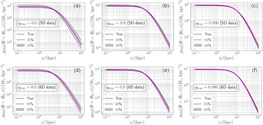
The same as Fig. D1 but for the reconstructed DM density profile ρ(R0, z) of the mock data.
D1.4 Dark matter density flattening
Fig. D3 shows the posterior distribution of q. We see that the posterior distribution is centred around qtrue, for both 5D and 6D mock data. This result implies that the lack of vlos is not a problem in inferring q as long as we handle the missing vlos properly.
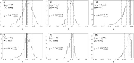
The posterior distribution of the DM density flattening q for the mock data. We note that the range of horizontal axis is different in each panel.
It is not surprising that the uncertainty in q is larger if we use 5D data instead of 6D data. This result indicates that the added information from vlos improves the inference on q, which is motivation to obtain vlos for a large number of Galactic RR Lyrae stars and other halo tracers (e.g. BHB and K-giants).
We note that the uncertainty in q is smaller when qtrue is larger. For example, for the 5D mock data sets, the difference between the 16th and 50th percentiles of the posterior distribution is Δq = 0.068, 0.042, and 0.014 for qtrue = 0.6, 0.8, and 0.996, respectively. This trend may be understood by considering that it is more difficult to distinguish the dynamical contributions from the baryonic disc and the DM halo if the DM halo is more flattened.
In this paper, we do not allow q > 1, because AGAMA can currently compute the actions only in oblate potentials. In Fig. D3(c)–(f), where qtrue = 0.996, the posterior distribution is skewed because our method cannot explore the parameter space at q > 1. It is worth noting that the posterior distribution of q is peaked at 0.99 < q < 1, consistent with qtrue = 0.996. This result is intriguing when we interpret our results with our fiducial model for which the posterior distribution is peaked at q = 1, (see Fig. 6a). Based on our analysis of mock data, our results with Gaia RR Lyrae stars might indicate that the Galactic DM halo is very close to spherical.
D2 Validation with realistic mock data generated from the m12m galaxy from the Latte simulations
D2.1 True shape of the dark matter halo of galaxy m12m
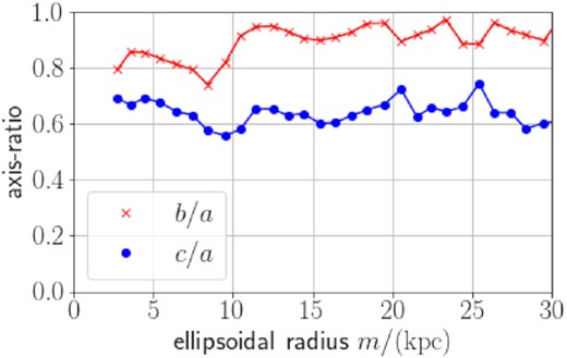
The minor-to-major axial ratio (c/a) and the intermediate-to-major axial ratio (b/a) as a function of the ellipsoidal radius m from the centre of m12m galaxy. We see that the inner part (|$m\lt 8\, \mathrm{kpc}$|) of the DM halo is triaxial, while it becomes nearly axisymmetric at |$m\gt 12 \, \mathrm{kpc}$|.
D2.2 Stellar distribution in m12m galaxy
The distribution of disc stars in m12m galaxy is nearly axisymmetric with no hint of a central bar. We fit the stellar distribution by a linear combination of three exponential discs, each of which can be described by equation (4). We refer to these three components as components 1, 2, and 3. The three parameters for component 1, the total mass, scale radius, and scale height are |$(M_\mathrm{disc,1}, R_\mathrm{d,1}, z_\mathrm{d,1}) = (2.30\times 10^{10}{\,\rm M_\odot} , 0.653 \, \mathrm{kpc}, 0.286 \, \mathrm{kpc})$|. Based on the short scale radius, the component 1 can be interpreted as the pseudo-bulge of the galaxy. (We note that pseudo-bulges have an exponential radial density profiles as shown in Kormendy & Kennicutt 2004, unlike the MW bulge model in our fiducial analysis.) The three parameters for components 2 and 3 are |$(M_\mathrm{disc,2}, R_\mathrm{d,2}, z_\mathrm{d,2}) = (8.27\times 10^{10}{\,\rm M_\odot} , 3.0 \, \mathrm{kpc}, 0.89 \, \mathrm{kpc})$| and |$(M_\mathrm{disc,3}, R_\mathrm{d,3}, z_\mathrm{d,3}) = (2.28\times 10^{10}{\,\rm M_\odot} , 5.8 \, \mathrm{kpc}, 2.78 \, \mathrm{kpc})$|, respectively. Based on the relative size of the scale heights, the components 2 and 3 can be interpreted as the thin and thick discs of m12m galaxy. We note that these structural parameters are at least partially consistent with the results in Sanderson et al. (2020).13
We use the functional forms of the above-mentioned three-component stellar distribution model in the mock analysis. We chose to treat (Mdisc, 1, Mdisc, 2, Rd, 2, Mdisc, 3, Rd, 3) as the free parameters to be determined through mock analysis. We chose to fix (Rd, 1, zd, 1, zd, 2, zd, 3) to their correct parameters mentioned in the previous paragraph. We note that these choices are designed to mimic our fiducial analysis. For example, we fixed zd, 2 in the mock analysis because the component 2 can be interpreted as the ‘thin disc’ of m12m and because the scale height of the MW’s thin disc is fixed in our fiducial analysis.
We also note that we adopted Bayesian priors for (Mdisc, 1, Mdisc, 2, Rd, 2, Mdisc, 3, Rd, 3) that are similar to the ones shown in Table 1. For example, we applied a Bayesian prior of Mdisc, 1 = (2.30 ± 0.23) × 1010M⊙, because the component 1 can be interpreted as the ‘bulge’ of m12m and because we adopted a 10 per cent uncertainty on the mass of the MW’s bulge in our fiducial analysis.
D2.3 Gas distribution in m12m galaxy
The distribution of the gas in m12m galaxy is approximately axisymmetric, with some hint of flocculent spiral-like structures. We use the distribution of the gas particles in m12m galaxy and compute the azimuthally averaged potential by using the AGAMA’s ‘CylSpline expansion’ scheme. Throughout the mock analysis, we use this ground-truth potential as the gas potential of m12m galaxy. This is motivated by the fact that we fixed the gas potential in our fiducial analysis.
D2.4 Mock data generated from Latte simulation
By using the star, gas, and DM particles in m12m galaxy, we evaluate the circular velocity curve and the radial profile of the vertical force at |$z=1.1 \, \mathrm{kpc}$| above the disc plane. We use these quantities to generate mock data for circular velocity curves and vertical force profiles akin to those shown in Figs 2 and 3 used in modelling the real RR Lyrae data.
To generate mock samples mimicking the RR Lyrae stars, we first select old halo stars in m12m with metallicity [Fe/H] < −1.5 and age |$\tau \gt 8 \, \mathrm{Gyr}$|. For these old halo stars, we add mock observational errors assuming that all the stars are RR Lyrae stars. As in Section D1.1, we prepare a 6D mock data set and a 5D mock data set without vlos data whose spatial distribution is defined in Section 3.3.
We use these mock halo catalogues along with the mock circular velocity curve and vertical force, to infer the DM density distribution in m12m in exactly the same manner as done for the Gaia RR Lyrae sample in the main body of this paper.
D2.5 Radial dark matter density of m12m galaxy
Fig. D5 shows the posterior distribution of the DM density profile at |$(R,z)=(R,0 \, \mathrm{kpc})$|. We see that ρDM(R, 0) is successfully reconstructed for |$1 \lesssim R \lesssim 100 \, \mathrm{kpc}$|. Given that we do not use mock halo stars within |$5 \, \mathrm{kpc}$| from the galactic centre, the successful recovery of the inner density profile of the DM halo is quite promising.
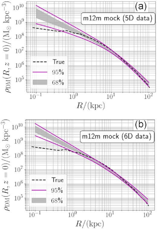
The same as Fig. D1 but using 5D and 6D mock data sets generated from m12m galaxy. The dashed line shows the true density profile |$\rho _\mathrm{DM}(R, z=0 \, \mathrm{kpc})$|, which is estimated from spherical harmonic expansion of the DM particles in m12m galaxy.
It seems to be challenging for our method to recover the DM density profile within |$1 \, \mathrm{kpc}$| from the galaxy. For example, Fig. D5 shows that the reconstructed profile has a steeper density slope than the true profile at |$R \lesssim 1 \, \mathrm{kpc}$|. This is not surprising, as we have seen in Fig. D1 that the reconstructed density profile at |$R\lesssim 1 \, \mathrm{kpc}$| is associated with large uncertainty even if the mock data are generated from a smooth halo model. This problem might be resolved by future access to halo stars within |$5 \, \mathrm{kpc}$| from the Galactic centre, however this is observationally challenging.
D2.6 Vertical dark matter density of m12m galaxy
Fig. D6 shows the posterior distribution of the DM density profile at (R, z) = (R0, z). We see that the global shape of ρDM(R0, z) is more or less well recovered, although there is some offset such that the reconstructed profile shows a lower density at low-|z| and the ‘knee’ of the recovered density profile occurs at slightly larger |z| than it should.
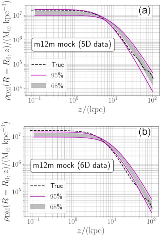
The same as Fig. D2 but using 5D and 6D mock data sets generated from m12m galaxy in Latte simulation. The dashed line shows the true density profile ρDM(R0, z), which is estimated from spherical harmonic expansion of the DM particles in m12m galaxy.
D2.7 Dark matter density flattening of m12m galaxy
Fig. D7 shows the posterior distribution of q. The three vertical dashed lines shows the (16,50,84)th percentiles of the distribution. We see that the posterior distribution has a width of ∼0.1 around its peak (|$q=0.765^{+0.111}_{-0.110}$| and |$q=0.818^{+0.103}_{-0.099}$| for 5D and 6D data, respectively), which is comparable to the result for the smooth-halo mock data analysis with qtrue = 0.6 (see Fig. D3a–d).

The true flattening of m12m DM halo is 0.55 < q < 0.7 (see the axial ratio (c/a) in Fig. D4). Thus, the median of the posterior distributions seen in Fig. D3 is systematically larger than it should be by ∼0.1−0.2. To understand the origin of this systematic offset, we show in Fig. D8 the correlation between the total stellar mass Mstar and the DM flattening q. The positive correlation between (q, Mstar) can be intuitively understood: If Mstar is overestimated, then the overall potential will become more flattened unless the DM halo becomes ‘less flattened’ to compensate. Thus, in our Bayesian analysis, the increase of Mstar is balanced by the increase of q. We speculate that our model favours a parameter set such that the stellar mass is larger than it should be, and that results in an overestimation of q. We have confirmed that our estimate of q in m12m’s DM halo can be improved (but not perfectly) if we fix the baryonic potential to the ground-truth potential computed from the particle distribution in m12m galaxy. At this moment, it is unclear why large (q, Mstar) is favoured in our analysis. It might be due to the disequilibrium of the halo, or due to the slight triaxiality of the DM halo (see Fig. D4). In any case, the lesson learned from this analysis is that it is important to have strong constraints on the baryonic mass distribution in order to accurately estimate q.
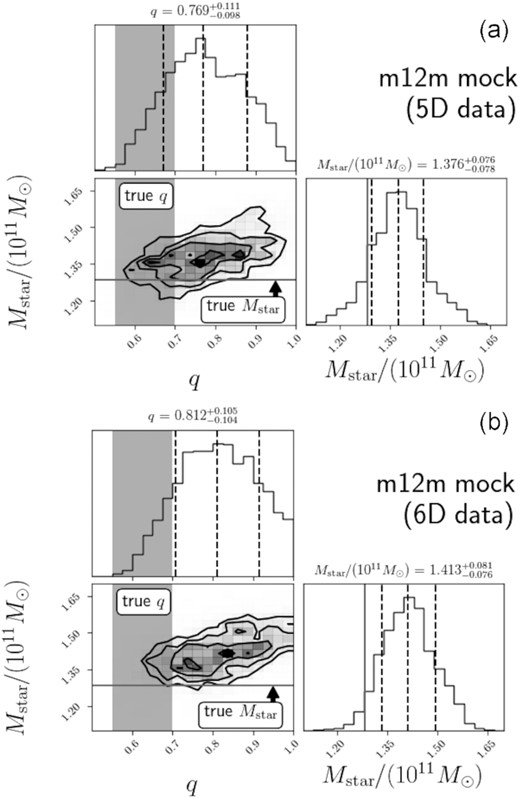
The correlation between the total stellar mass Mstar and the DM density flattening q seen in the posterior distribution of the mock analysis of m12m galaxy. The correct value of q is 0.55 < q < 0.7, which is shown by a grey vertical band in the left-hand panels. The correct value of Mstar is Mstar = 1.28 × 10¹¹M⊙, which is shown as the horizontal solid line in lower left-hand corner and as the vertical solid line in the lower right-hand corner of each panel.
APPENDIX E: A NOTE ON GAIA EDR3
In this paper, we have used the proper motion data from Gaia DR2. Just before we complete this work, Gaia EDR3 was released (Gaia Collaboration 2021). We found that the uncertainty in proper motion data for our RR Lyrae star sample is reduced by a factor of ∼2, almost independent of their mean G-magnitude. We think the main conclusion of our paper will not be changed if we use Gaia EDR3 data instead of Gaia DR2 data, because the dominant sources of uncertainty in our analysis is the uncertainty in the photometric distance of RR Lyrae stars and the lack of vlos data, both of which will not be improved by Gaia EDR3.
