Bayesian analysis of quasar light curves with a running optimal average: new time delay measurements of COSMOGRAIL gravitationally lensed quasars

Donnan, Fergus R; Horne, Keith; Hernández Santisteban, Juan V

doi:10.1093/mnras/stab2832

ABSTRACT

We present a new method of modelling time-series data based on the running optimal average (ROA). By identifying the effective number of parameters for the ROA model, in terms of the shape and width of its window function and the times and accuracies of the data, we enable a Bayesian analysis, optimizing the ROA width, along with other model parameters, by minimizing the Bayesian information criterion (BIC) and sampling joint posterior parameter distributions using MCMC methods. For analysis of quasar light curves, our implementation of ROA modelling can measure time delays among light curves at different wavelengths or from different images of a lensed quasar and, in future work, be used to inter-calibrate light-curve data from different telescopes and estimate the shape and thus the power-density spectrum of the light curve. Our noise model implements a robust treatment of outliers and error-bar adjustments to account for additional variance or poorly quantified uncertainties. Tests with simulated data validate the parameter uncertainty estimates. We compare ROA delay measurements with results from cross-correlation and from javelin, which models light curves with a prior on the power-density spectrum. We analyse published COSMOGRAIL light curves of multilensed quasar light curves and present the resulting measurements of the inter-image time delays and detection of microlensing effects.

gravitational lensing: strong, methods: data analysis, quasars: general

1 INTRODUCTION

Active galactic nuclei (AGN) are powered by accretion on to a super-massive black hole (SMBH), producing the brightest persistent objects in the Universe (e.g. Salpeter 1964; Lynden-Bell 1969; Sanders et al. 1989). AGN are known to play a key role across cosmic time in the evolution of galaxies (e.g. Fabian 2012; Heckman & Best 2014), and so understanding the central regions that power AGN is crucial. Despite their extreme brightness, resolving structure close to the black hole remains a challenge. Spatially resolving these regions typically requires sub-microacrsecond resolution, a feat outwith the spatial resolution of current telescopes. Recent progress has been made relying on interferometry with instruments such as GRAVITY in the near-IR (Gravity Collaboration 2018) resolving the the broad-line region (BLR) on sub-pc scales, or the Event Horizon Telescope (Event Horizon Telescope Collaboration 2019) resolving the shadow of the SMBH at the centre of M87.

AGN are known to be variable (e.g. Kawaguchi et al. 1998; Dexter & Agol 2011), and while its physical origin is not fully understood, this variability can be exploited to probe the inner regions of AGN. Echo mapping or reverberation mapping (e.g. Blandford & McKee 1982; Peterson 1993; Cackett, Bentz & Kara 2021) is a technique that exploits this variability as well as the finite traveltime of light to dissect the accretion flow, providing a probe of the structure on a scale equivalent to sub-microarcsecond resolution. This technique is based upon variable X-ray/EUV emission originating close to the BH, that propagates outward at the speed of light and is reprocessed, either as thermal continuum emission from the disc or as broad emission lines from the BLR.

The main aim of reverberation mapping experiments is to measure the time delay between variations in the driving and reprocessed light curves. In the case of thermal reprocessing in the accretion disc, the wavelength is set by the local temperature, therefore measuring the time delays as a function of wavelength, provides a test of the temperature structure of the disc as well as the size of the disc (Cackett, Horne & Winkler 2007). Measuring the delay of the response of broad emission lines, provides an estimate of the size of the BLR and thus the mass of the BH (e.g. Peterson et al. 2004). Measuring the response of these broad lines as a function of velocity, allows the structure and kinematics of the BLR to be investigated (Horne et al. 2004). For these experiments, a robust method of measuring these time delays is required.

Time delays can also be measured between images of gravitationally lensed quasars by similarly exploiting the intrinsic variability. These can provide a direct probe of Hubble’s constant, H₀ (e.g. Tewes et al. 2012), measure the size of the BLR of the source quasar (e.g. Sluse & Tewes 2014) and enable reverberation mapping at high redshift through reconstructing rest frame light curves (e.g. Williams et al. 2021). Measuring these time delays also requires accounting for microlensing effects that vary the brightness of the lensed images on a longer time-scale than the intrinsic quasar variability (e.g. Tewes, Courbin & Meylan 2013).

Typically, time delays between two light curves have been measured using the interpolation cross-correlation function (ICCF; Gaskell & Peterson 1987). The most notable problem with this method is that it is based upon interpolating one light curve and treating this as the driver to measure the delay to another. This is especially a problem for unevenly sampled data or large gaps where observations may have been halted for a period of time, often resulting in poor constraints on these time delays. An alternative approach would be to model the light curves based on some assumptions. The most popular of these, javelin (Zu, Kochanek & Peterson 2011), models the variability with a damped random walk, and generally provides tighter uncertainties (e.g. Yu et al 2020) on the measured delays as well as provides a model of the driving light curve. A similar approach is taken by cream (Starkey, Horne & Villforth 2016), which models the light curves based on the ‘lamp-post’ model, inferring the driving light curve.

In this paper, we investigate using a running optimal average (ROA) to model AGN light curves and to then measure the time delays between light curves. We present the code pyroa,¹ which draws information from all available light-curve data in forming the ROA model of the AGN variations. The ROA is then normalized, shifted, and scaled to fit the individual light curves, thus measuring the mean and rms of the variations in each light curve, and the time delays between them. Markov chain Monte Carlo (MCMC) samples provide parameter estimates and uncertainties. In Section 2, we outline the running optimal average and the modelling process of pyroa to measure inter-light-curve delays. In Section 3, we test the method with simulated data. In Section 4, we use our method to measure inter-image delays of gravitationally lensed quasars of public data from the COSMOGRAIL project (Eigenbrod et al. 2005, and references therein). We conclude in Section 5 with a brief summary of our findings.

2 LIGHTCURVE MODELLING

This section outlines a Bayesian analysis using a running optimal average (ROA) to model light-curve data. The ROA model represents the light curve as a running optimal average of the data. The Bayesian information criterion (BIC) is then used to tune the degree of smoothing warranted by the data. The model parameters are sampled with MCMC to estimate their values and uncertainties. Unlike methods such as cross-correlation that compare one light curve with another, the ROA model fits multiple light-curve data sets simultaneously to collect all the available information in determining the light-curve shape.

2.1 Running optimal average

The ROA model provides a smooth differentiable function that describes the shape of a light curve, or other time series, along with an error envelope to quantify its uncertainty. It is defined as follows. Consider time-series data consisting of N data points D_i, with error bars σ_i, at times t_i. The ROA model light curve X(t) is an optimal (inverse-variance weighted) average of all the data, evaluated at time t with a window function that diminishes the influence of data at times t_i that are far from the time t. This is given by

$$\begin{eqnarray*} X(t) = \frac{\sum _{i=1}^{N} D_i w_i(t)}{\sum _{i=1}^{N} w_i(t)} \ , \quad w_i(t) = \frac{1}{\sigma _i^2} \exp \left[-\frac{1}{2} \left(\frac{t - t_i}{\Delta }\right) ^2 \right] \ , \end{eqnarray*}$$

(1)

where the weights w_i(t) are described here by a Gaussian window function with width Δ. Given the uncertainties σ_i on the data D_i, the resulting statistical variance of the running optimal average is

$$\begin{eqnarray*} \sigma ^2 \left[X(t)\right] = \frac{1}{\sum _{i=1}^{N} w_i(t)}. \end{eqnarray*}$$

(2)

This defines the error envelope for the ROA light-curve model. When data points are densely sampling compared with the window width Δ, they are averaged with optimal inverse-variance weights. The ROA interpolates across data gaps, and extrapolates beyond the ends of the data, with an error envelope that expands appropriately, depending on the adopted shape of the window function.

Unlike other attempts to model quasar variability, the ROA does not make any assumptions about the shape of the driving light curve. For example, javelin uses a damped random walk that is then smoothed by a uniform transfer function to model the light curves, whereas the ROA simply calculates the shape from the data, which is already smoothed. This provides a unique insight into quasar variability compared to previous methods.

2.1.1 Window function shape

The ROA can be defined in terms of a generic window function shape W(x), where x ≡ (t − t_i)/Δ, and we require W(0) = 1 and W(± ∞) = 0. Perhaps the simplest option is the‘top-hat’ window function,

$$\begin{eqnarray*} W(x) \equiv \left\lbrace \begin{array}{cc}1\ , & |x| \ \lt \ 1 \ , \\ 0\ , & |x| \ \gt \ 1 \ . \end{array} \right. \ \end{eqnarray*}$$

(3)

This admits data within a time interval ±Δ. Although widely used, the resulting ROA X(t) jumps whenever data enter or leave the window, and the uncertainty σ[(X(t)] is infinite whenever a data gap exceeds the window width |$2\, \Delta$|⁠. These undesirable features are avoided with smoothly-declining window functions such as a Gaussian window function,

$$\begin{eqnarray*} W(x) \equiv \exp {\left(- \frac{ x^2 }{2 \, \Delta }\right)} \ . \end{eqnarray*}$$

(4)

Other shapes with wider wings affect the rate at which data more distant in time lose influence on the ROA. For example, an inverse-cosh window function,

$$\begin{eqnarray*} W(x) \equiv \frac{ 1 }{\cos{\it h} {(x)}} \ , \end{eqnarray*}$$

(5)

has exponentially decaying wings, and a Lorentzian window function,

$$\begin{eqnarray*} W(x) \equiv \frac{ 1 }{ 1+x^2 } \ , \end{eqnarray*}$$

(6)

has power-law x⁻² wings. Other choices are clearly possible.

2.1.2 Effective number of parameters

The ‘flexibility’ of the ROA is controlled by the window function width Δ. If Δ is small, then X(t) is flexible enough to follow relatively rapid variations in the data. If Δ is large, then X(t) is stiffer and can follow only slower variations. In the limit Δ → ∞, the ROA model becomes a rigid constant, the optimal average of all the data. From this, it is clear that the value of Δ controls the effective number of parameters of the model. A small Δ highly flexible ROA model has many parameters. As Δ → ∞, the number of parameters reduces to just 1. As Δ → 0, X(t) can fit the data perfectly, and thus in this limit the number of parameters becomes N, the number of data points.

Optimizing Δ is important because an overly-stiff model fails to fit the data while an overly-flexible model overfits the noisy data. The balance between overfitting and underfitting can be achieved by a trade-off between the quality of the fit, as measured for example by χ², and an Occam bias favouring simpler models with relatively few parameters. To implement this, we need to quantify the effective number of parameters for a given value of Δ.

The number of parameters P_i used by the ROA model X(t) to fit a single datum D_i ± σ_i at time t_i is given by

$$\begin{eqnarray*} P_i (\Delta) = \frac{\partial X(t_i)}{\partial D_i} = \frac{w_i(t)}{\sum _k w_k(t_i)} = \frac{1/{\sigma _i^2}}{\sum _k \frac{1}{\sigma _k^2} \exp \left[-\frac{1}{2} \left(\frac{t_i - t_k}{\Delta }\right) ^2 \right]}\ , \end{eqnarray*}$$

(7)

written here for a Gaussian window function. Note that P_i = 1 for an isolated data point with no other data close enough to affect the ROA. In a more densely sampled region, P_i decreases to the data point’s share of the inverse-variance weights of all data close enough in time to contribute to the ROA. For the full ROA model, X(t), the total number of parameters sums the previous equation for P_i over all N data points:

$$\begin{eqnarray*} P_X (\Delta) = \sum _{i=1}^N P_i = \sum _{i=1}^N \frac{1/{\sigma _i^2}}{\sum _k \frac{1}{\sigma _k^2} \exp \left[-\frac{1}{2} \left(\frac{t_i - t_k}{\Delta }\right) ^2 \right]}\ . \end{eqnarray*}$$

(8)

Knowing the number of parameters allows for the optimal value of Δ to be determined using the BIC. This is a ‘badness of fit’ statistic that includes a penalty for models with too many parameters. We have released the code for simply calculating the running optimal average separately to the pyroa code for modelling the light curves. This code, roa,² calculates the running optimal average and effective number of parameters for some given data.

2.2 Simple model

The simplest model for these light curves is one where the driving light curve is scaled, shifted, and translated in time to reproduce the flux of a given light curve, i. The following is an equation for the model flux as a function of time, f_i(t), given by

$$\begin{eqnarray*} f_{i}(t) = A_{i}X\left(t - \tau _{i}\right) + B_{i} \ , \end{eqnarray*}$$

(9)

where A_i represents the rms flux, B_i represents the mean flux, τ_i represents the time delay, and X(t) is the driving light curve. The time delay for the first light curve is fixed at 0 (τ₁ = 0), which means that the time delays are measured relative to this light curve.

In this simple model the assumption is that the shape of the variability given by X(t), is the same for each light curve, calculated using all of the light curves shifted and stacked appropriately where the ROA is calculated from equation (1). This provides the maximum information for determining the shape of the driving light curve. In this model, we can also add an extra variance term to the noise model as a free parameter for each light curve, to account for additional uncertainty not included in the original error bars.

We fit this model using a Bayesian approach where the posterior probability of the model, M, given the data, D, (Pr(M|D)) is maximized by the best-fitting parameters. The natural log of this probability is given by the sum of the log prior (Pr(M)) and the log-likelihood (Pr(D|M)):

$$\begin{eqnarray*} \ln {\textrm {Pr}(M|D)}= \ln {\textrm {Pr}(M)} + \ln {\textrm {Pr}(D|M)} + \textrm {const} \ . \end{eqnarray*}$$

(10)

As mentioned previously, fitting this model required the use of a statistic that includes a penalty for a running optimal average that is too flexible. As the BIC is a ‘badness of fit’ statistic, it is minimized by the best-fitting parameters. The BIC is given by

$$\begin{eqnarray*} \textrm {BIC} = -2\ln {\textrm {Pr}(D|M)} + P\ln {N} \ , \end{eqnarray*}$$

(11)

where the second term is the penalty, added to negative twice the log likelihood, which depends on the number of parameters, P, and the total number of data points, N. For our model, the first term is

$$\begin{eqnarray*} {-}2\ln {\textrm {Pr}(D|M)} = \sum _{i=1}^{N_l} \left[ \sum _{j=1}^{N_i} \left[ \frac{\left(D_{j, i} - f_i\right)^2}{\sigma _{j, i}^2 + s_{i}^2 } + \ln \left(\frac{\sigma _{j, i}^2 + s_{i}^2}{\sigma _{j, i}^2}\right) \right] \right] , \nonumber \\ \end{eqnarray*}$$

(12)

where for N_l light curves, indexed i = 1, 2, 3, ..., each contain N_i data points, D_{j, i}, with errors, σ_{j, i}. The extra error parameters, s_i, are added in quadrature to the original error bars. The right-hand term of this equation provides a penalty for adding additional variance to the flux error measurements, which is measured relative to the original error bars to give zero when no extra variance is added.

The penalty term for the number of parameters is given by

$$\begin{eqnarray*} P\ln {N} = \sum _{i=1}^{N_l} 4\ln (N_{i}) + P_X\ln \left(\sum _{i=1}^{N_l} N_{i} \right) \ . \end{eqnarray*}$$

(13)

The first term features a factor of 4, for the four parameters per light curve: A_i, B_i, τ_i, s_i. The number of parameters in the final term, P_X, depends on the free parameter Δ, according to equation (8). This ensures that the best-fitting running optimal average is the one that fits the data well with the fewest effective number of parameters.

2.3 Fitting procedure

To determine the best-fitting parameters for this model, we use the MCMC package, emcee (Foreman-Mackey et al. 2013). This process samples the posterior probability of the model given the data, including prior probabilities for the parameters. The priors are chosen as uniform distributions between sensible limits, e.g. A_i is known to be positive. For each sample in the MCMC, the following steps are taken to calculate the posterior probability:

First, each light curve is shifted by the appropriate parameters. This means each data point, D_{j, i}, is altered such that D_{j, i} → (D_{j, i} − B_i)/A_i and is shifted back in time by τ_i. This has the effect of ‘stacking’ the light curves (if the parameters are close to optimal), allowing for the running optimal average to be determined. The first light curve is not shifted in time ensuring that the ‘stacking’ occurs on light curve 1. This means the time delays are measured relative to this light curve that removes a degeneracy in the time delays. Without this, there is no reference to measure a lag from and therefore the τ_i parameters would be degenerate.
The extra error parameters, s_i, are also added in quadrature to the error bars of each light curve, i.e. |$\sigma _{j, i} \rightarrow \sqrt{\sigma _{j, i}^2 + s_i^2}$|⁠.
The shifted light curves are then merged into a single light curve, where the running optimal average, X(t), is calculated on a fine grid of times using equation (1). The grid consists of 1000 equally spaced points, ranging over the initial and final times of the merged light curve. The effective number of parameters given the value of Δ, is also calculated using equation (8).
The running optimal average, X(t), is then normalized to ensure that |$\langle X \rangle _t=0, \, \langle X^2 \rangle _t=1$|⁠. This is done by subtracting the mean of X(t), and then dividing by the standard deviation of X(t).
The model is then calculated for each light curve, using equation (9).
Finally, the BIC is calculated using equation (11). The negative of the BIC provides twice the log likelihood plus a penalty, therefore the relative log posterior probability is calculated by adding the twice the log prior to the negative of the BIC. i.e. 2ln Pr(M) − BIC. This is the statistic calculated for each sample of the Markov chain, and maximized by the best-fitting solution.

This process is repeated for a large number of samples, discarding a fraction of samples as ‘burn-in’. The best-fitting parameters are chosen by taking the median of the posterior distributions, with uncertainties in the range from the 16th to the 84th percentile. The starting positions of the MCMC walkers are chosen as Gaussian random numbers centred on a chosen value. For the parameter A_i, the walkers are started around the rms of the individual light curves. For B_i, they are started around the mean of the individual light curves and for Δ they are started around 1 d – although this value can be altered depending on the data. The other parameters were started around zero. The initial time delays and Δ can be chosen depending on the data being modelled. For example, if the time delay is large and can be estimated visually (or by some other method), initializing the walkers by this estimation will reduce the ‘burn-in’ required and/or prevent the Markov chain getting stuck in a local minima.

2.4 Managing outliers

A major problem with astronomical data are outliers, caused by external processes such as cosmic rays. The optimal process of managing them is often unclear as there are many approaches. A common method is sigma clipping, where data points outwith a certain threshold (Nσ) of the model, are excluded. For example, if a datum were outside a threshold of 3σ, it lies outwith a probability of 99.7 per cent, assuming Gaussian error bars.

Sigma clipping has the effect of creating a discontinuity in χ² at the threshold, as χ² drops to zero beyond the threshold. This discontinuity is undesirable as a data point slightly outwith the threshold is treated vastly differently to one slightly within the threshold. The most simple way to resolve this issue is to instead have the χ² to become constant at the value of the threshold, demonstrated in Fig. 1. This is equivalent to expanding the error bars of the outliers such that they are exactly Nσ away from the model. This method of sigma clipping was implemented into the fitting process when calculating the BIC, where we treat the χ² term of equation (12) as a piecewise function that is constant for data beyond the threshold. The second term is handled by expanding the error bars of points outwith the threshold to meet Nσ, i.e. |$\sigma _{j, i}^2 + s_{i}^2$| is set to the variance required such that the datum is exactly Nσ from the model.

Demonstration of sigma clipping at a threshold of 4σ. The value of χ2 is constant beyond the threshold, shown by the solid line. The dashed blue line shows χ2 without any sigma clipping.

Figure 1.

Demonstration of sigma clipping at a threshold of 4σ. The value of χ² is constant beyond the threshold, shown by the solid line. The dashed blue line shows χ² without any sigma clipping.

Open in new tab Download slide

Other methods of sigma clipping are also possible. While χ² is no longer discontinuous as the threshold, the first derivative is still discontinuous. A way to solve this issue would be for χ² to become linear with the gradient set by the first derivative evaluated at the threshold. This is effectively converting χ² into a function similar to the median absolute deviation (MAD) beyond the threshold, which is much more resilient to outliers than χ². Implementing such a solution would be relatively straightforward, if required in future applications of the model.

3 TESTING WITH MOCK DATA

To ensure the ROA model and fitting procedure is robust, we tested our algorithm with mock data where the variability is generated from a random walk. A damped random walk has been shown to describe quasar variability well (e.g. Kozłowski et al. 2010; MacLeod et al. 2010), where the variability is given by a random walk on short time-scales but ‘damped’ on long time-scales to push deviations towards the mean, with typical damping time-scales on the order ∼200 d (MacLeod et al. 2010). For our simulation, we use a dimensionless duration of 50 and delays of 5 and 10, which, if measured in days, are plausible delays for reverberation mapping studies of BLR emission line lags (e.g. Grier et al. 2017) or accretion disc lags (e.g. Homayouni et al. 2021). Therefore, it is suitable to use a random walk for 50 d as this is significantly shorter than the typical damping time-scale of ∼200 d. We first generated three mock light curves based on the same random walk where each is shifted in time by some true parameter. This allows us to test our method’s ability to reproduce the true value of the parameters. The mock data was generated by the following:

A random walk light curve was generated where each step is a Gaussian random number with a mean of 0 and a standard deviation of 1. This was done for 10 000 steps over a range of times from 0 to 100. The random walk was then normalized such that its mean is 0 and rms is 1. This mimics the random variability of an AGN and an example is plotted in the top panel of Fig. 2 in purple.
A set of discrete times was generated between 30 and 70 with equal spacing, consisting of 200 points for the first light curves, 150 for the second, and 250 points for the third. A Gaussian random number with a mean of 0 and a standard deviation of 1 was then multiplied by the spacing between the times and added to the original times. This makes the spacing between the data points uneven.
The normalized random walk was then scaled and shifted in time by the true parameters (shown in Table 1), and calculated at the times generated in the previous step.
To simulate error bars, errors were chosen as some arbitrary value plus a small uniform random number to vary the sizes of the error bars across the light curve.
To scatter the flux values based on the error bars, they were calculated as Gaussian random numbers with a mean calculated in the second step and a standard deviation given by the error bars.

Figure 2.

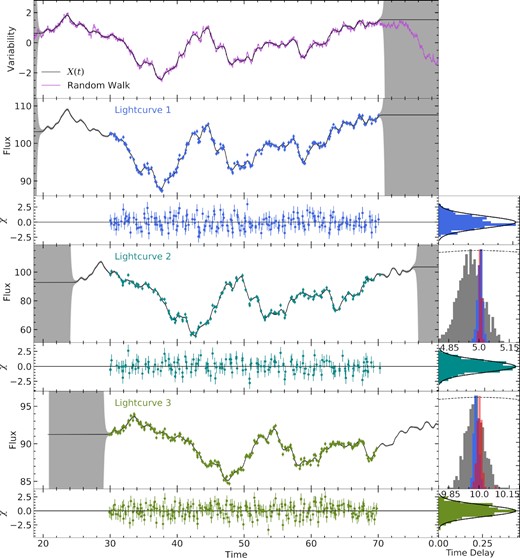
Model fit to mock data, Case A. The top panel shows the random walk used to generate the data (purple) overlayed with the normalized driving light curve found by the model (black). The grey shaded region shows the error envelope for the running optimal average calculated using equation (2). The three mock light curves are plotted in the following panels, overlayed with the best-fitting model in black. The normalized residuals, χ, for each light curve are also shown, with the colour corresponding to the appropriate light curve. The right-hand panels of each light curve show histograms of the probability distributions for the time delay. The cross-correlation centroid distribution is shown in grey, our method (pyroa) is shown in blue and javelin is shown in red. The dashed line shows the cross-correlation function. The right-hand panels of the residuals show a histogram of those normalized residuals, in comparison with the expected Gaussian distribution in black.

Open in new tab Download slide

Table 1.

Open in new tab

Mock data results.

Parameter	Truth	Prior	Best fit	ICCF	javelin
Case A: high signal-to-noise ratio (Fig. 2)
A₁	5.0	[0, 20]	\|$4.954^{+0.035}_{-0.035}$\|	–	–
A₂	12.0	[0, 20]	\|$12.04^{+0.10}_{-0.10}$\|	–	–
A₃	2.0	[0, 20]	\|$2.003^{+0.014}_{-0.014}$\|	–	–
B₁	100.0	[0, 1000]	\|$100.000^{+0.033}_{-0.035}$\|	–	–
B₂	85.0	[0, 1000]	\|$85.186^{+0.093}_{-0.096}$\|	–	–
B₃	90.0	[0, 1000]	\|$90.003^{+0.014}_{-0.014}$\|	–	–
s₁	0.0	[0, 10]	\|$0.509^{+0.027}_{-0.026}$\|	–	–
s₂	0.0	[0, 10]	\|$1.322^{+0.078}_{-0.069}$\|	–	–
s₃	0.0	[0, 10]	\|$0.197^{+0.013}_{-0.013}$\|	–	–
τ₂	5.0	[−50, 50]	\|$5.006^{+0.011}_{-0.013}$\|	\|$4.958^{+0.058}_{-0.062}$\|	\|$5.0061^{+0.0059}_{-0.0052}$\|
τ₃	10.0	[−50, 50]	\|$9.986^{+0.013}_{-0.010}$\|	\|$9.991^{+0.048}_{-0.040}$\|	\|$10.002^{+0.012}_{-0.011}$\|
Δ	–	[0.1, 10]	\|$0.239^{+0.010}_{-0.010}$\|	–	–
Case B: seasonal gaps (Fig. 4)
A₁	5.0	[0, 20]	\|$4.953^{+0.043}_{-0.043}$\|	–	–
A₂	12.0	[0, 20]	\|$12.57^{+0.18}_{-0.17}$\|	–	–
A₃	2.0	[0, 20]	\|$1.990^{+0.018}_{-0.018}$\|	–	–
B₁	100.0	[0, 1000]	\|$99.915^{+0.047}_{-0.048}$\|	–	–
B₂	85.0	[0, 1000]	\|$84.84^{+0.11}_{-0.11}$\|	–	–
B₃	90.0	[0, 1000]	\|$90.075^{+0.020}_{-0.020}$\|	–	–
s₁	0.0	[0, 10]	\|$0.396^{+0.031}_{-0.030}$\|	–	–
s₂	0.0	[0, 10]	\|$0.956^{+0.100}_{-0.093}$\|	–	–
s₃	0.0	[0, 10]	\|$0.172^{+0.020}_{-0.020}$\|	–	–
τ₂	5.0	[−50, 50]	\|$5.009^{+0.018}_{-0.013}$\|	\|$4.20^{+0.17}_{-0.15}$\|	\|$5.016^{+0.017}_{-0.019}$\|
τ₃	10.0	[−50, 50]	\|$9.993^{+0.021}_{-0.024}$\|	\|$8.56^{+0.18}_{-0.20}$\|	\|$10.037^{+0.049}_{-0.048}$\|
Δ	–	[0.1, 10]	\|$0.206^{+0.013}_{-0.012}$\|	–	–
Case C: low signal-to-noise ratio (Fig. 5)
A₁	5.0	[0, 20]	\|$4.35^{+0.19}_{-0.19}$\|	–	–
A₂	12.0	[0, 20]	\|$11.82^{+0.59}_{-0.55}$\|	–	–
A₃	2.0	[0, 20]	\|$2.13^{+0.16}_{-0.16}$\|	–	–
B₁	100.0	[0, 1000]	\|$99.93^{+0.18}_{-0.19}$\|	–	–
B₂	85.0	[0, 1000]	\|$85.43^{+0.57}_{-0.56}$\|	–	–
B₃	90.0	[0, 1000]	\|$89.83^{+0.16}_{-0.16}$\|	–	–
s₁	0.0	[0, 10]	\|$0.44^{+0.34}_{-0.30}$\|	–	–
s₂	0.0	[0, 10]	\|$3.09^{+0.66}_{-0.71}$\|	–	–
s₃	0.0	[0, 10]	\|$0.77^{+0.30}_{-0.39}$\|	–	–
τ₂	5.0	[−50, 50]	\|$5.31^{+0.14}_{-0.15}$\|	\|$5.30^{+0.27}_{-0.32}$\|	\|$5.30^{+0.17}_{-0.15}$\|
τ₃	10.0	[−50, 50]	\|$10.16^{+0.23}_{-0.22}$\|	\|$10.30^{+0.45}_{-0.47}$\|	\|$10.22^{+0.24}_{-0.23}$\|
Δ	–	[0.1, 10]	\|$1.45^{+0.11}_{-0.10}$\|	–	–
Case D: high S/N with underestimated errors (Fig. 6)
A₁	5.0	[0, 20]	\|$4.965^{+0.034}_{-0.034}$\|	–	–
A₂	12.0	[0, 20]	\|$11.787^{+0.089}_{-0.093}$\|	–	–
A₃	2.0	[0, 20]	\|$2.003^{+0.013}_{-0.013}$\|	–	–
B₁	100.0	[0, 1000]	\|$99.962^{+0.032}_{-0.031}$\|	–	–
B₂	85.0	[0, 1000]	\|$85.072^{+0.085}_{-0.089}$\|	–	–
B₃	90.0	[0, 1000]	\|$90.001^{+0.013}_{-0.013}$\|	–	–
s₁	0.16	[0, 10]	\|$0.525^{+0.024}_{-0.023}$\|	–	–
s₂	0.42	[0, 10]	\|$1.212^{+0.066}_{-0.063}$\|	–	–
s₃	0.15	[0, 10]	\|$0.2478^{+0.0098}_{-0.0091}$\|	–	–
τ₂	5.0	[−50, 50]	\|$4.992^{+0.011}_{-0.013}$\|	\|$4.951^{+0.056}_{-0.059}$\|	\|$5.006^{+0.036}_{-0.012}$\|
τ₃	10.0	[−50, 50]	\|$9.974^{+0.013}_{-0.013}$\|	\|$9.993^{+0.041}_{-0.038}$\|	\|$9.975^{+0.042}_{-0.238}$\|
Δ	–	[0.1, 10]	\|$0.22^{+0.10}_{-0.10}$\|	–	–

Parameter	Truth	Prior	Best fit	ICCF	javelin
Case A: high signal-to-noise ratio (Fig. 2)
A₁	5.0	[0, 20]	\|$4.954^{+0.035}_{-0.035}$\|	–	–
A₂	12.0	[0, 20]	\|$12.04^{+0.10}_{-0.10}$\|	–	–
A₃	2.0	[0, 20]	\|$2.003^{+0.014}_{-0.014}$\|	–	–
B₁	100.0	[0, 1000]	\|$100.000^{+0.033}_{-0.035}$\|	–	–
B₂	85.0	[0, 1000]	\|$85.186^{+0.093}_{-0.096}$\|	–	–
B₃	90.0	[0, 1000]	\|$90.003^{+0.014}_{-0.014}$\|	–	–
s₁	0.0	[0, 10]	\|$0.509^{+0.027}_{-0.026}$\|	–	–
s₂	0.0	[0, 10]	\|$1.322^{+0.078}_{-0.069}$\|	–	–
s₃	0.0	[0, 10]	\|$0.197^{+0.013}_{-0.013}$\|	–	–
τ₂	5.0	[−50, 50]	\|$5.006^{+0.011}_{-0.013}$\|	\|$4.958^{+0.058}_{-0.062}$\|	\|$5.0061^{+0.0059}_{-0.0052}$\|
τ₃	10.0	[−50, 50]	\|$9.986^{+0.013}_{-0.010}$\|	\|$9.991^{+0.048}_{-0.040}$\|	\|$10.002^{+0.012}_{-0.011}$\|
Δ	–	[0.1, 10]	\|$0.239^{+0.010}_{-0.010}$\|	–	–
Case B: seasonal gaps (Fig. 4)
A₁	5.0	[0, 20]	\|$4.953^{+0.043}_{-0.043}$\|	–	–
A₂	12.0	[0, 20]	\|$12.57^{+0.18}_{-0.17}$\|	–	–
A₃	2.0	[0, 20]	\|$1.990^{+0.018}_{-0.018}$\|	–	–
B₁	100.0	[0, 1000]	\|$99.915^{+0.047}_{-0.048}$\|	–	–
B₂	85.0	[0, 1000]	\|$84.84^{+0.11}_{-0.11}$\|	–	–
B₃	90.0	[0, 1000]	\|$90.075^{+0.020}_{-0.020}$\|	–	–
s₁	0.0	[0, 10]	\|$0.396^{+0.031}_{-0.030}$\|	–	–
s₂	0.0	[0, 10]	\|$0.956^{+0.100}_{-0.093}$\|	–	–
s₃	0.0	[0, 10]	\|$0.172^{+0.020}_{-0.020}$\|	–	–
τ₂	5.0	[−50, 50]	\|$5.009^{+0.018}_{-0.013}$\|	\|$4.20^{+0.17}_{-0.15}$\|	\|$5.016^{+0.017}_{-0.019}$\|
τ₃	10.0	[−50, 50]	\|$9.993^{+0.021}_{-0.024}$\|	\|$8.56^{+0.18}_{-0.20}$\|	\|$10.037^{+0.049}_{-0.048}$\|
Δ	–	[0.1, 10]	\|$0.206^{+0.013}_{-0.012}$\|	–	–
Case C: low signal-to-noise ratio (Fig. 5)
A₁	5.0	[0, 20]	\|$4.35^{+0.19}_{-0.19}$\|	–	–
A₂	12.0	[0, 20]	\|$11.82^{+0.59}_{-0.55}$\|	–	–
A₃	2.0	[0, 20]	\|$2.13^{+0.16}_{-0.16}$\|	–	–
B₁	100.0	[0, 1000]	\|$99.93^{+0.18}_{-0.19}$\|	–	–
B₂	85.0	[0, 1000]	\|$85.43^{+0.57}_{-0.56}$\|	–	–
B₃	90.0	[0, 1000]	\|$89.83^{+0.16}_{-0.16}$\|	–	–
s₁	0.0	[0, 10]	\|$0.44^{+0.34}_{-0.30}$\|	–	–
s₂	0.0	[0, 10]	\|$3.09^{+0.66}_{-0.71}$\|	–	–
s₃	0.0	[0, 10]	\|$0.77^{+0.30}_{-0.39}$\|	–	–
τ₂	5.0	[−50, 50]	\|$5.31^{+0.14}_{-0.15}$\|	\|$5.30^{+0.27}_{-0.32}$\|	\|$5.30^{+0.17}_{-0.15}$\|
τ₃	10.0	[−50, 50]	\|$10.16^{+0.23}_{-0.22}$\|	\|$10.30^{+0.45}_{-0.47}$\|	\|$10.22^{+0.24}_{-0.23}$\|
Δ	–	[0.1, 10]	\|$1.45^{+0.11}_{-0.10}$\|	–	–
Case D: high S/N with underestimated errors (Fig. 6)
A₁	5.0	[0, 20]	\|$4.965^{+0.034}_{-0.034}$\|	–	–
A₂	12.0	[0, 20]	\|$11.787^{+0.089}_{-0.093}$\|	–	–
A₃	2.0	[0, 20]	\|$2.003^{+0.013}_{-0.013}$\|	–	–
B₁	100.0	[0, 1000]	\|$99.962^{+0.032}_{-0.031}$\|	–	–
B₂	85.0	[0, 1000]	\|$85.072^{+0.085}_{-0.089}$\|	–	–
B₃	90.0	[0, 1000]	\|$90.001^{+0.013}_{-0.013}$\|	–	–
s₁	0.16	[0, 10]	\|$0.525^{+0.024}_{-0.023}$\|	–	–
s₂	0.42	[0, 10]	\|$1.212^{+0.066}_{-0.063}$\|	–	–
s₃	0.15	[0, 10]	\|$0.2478^{+0.0098}_{-0.0091}$\|	–	–
τ₂	5.0	[−50, 50]	\|$4.992^{+0.011}_{-0.013}$\|	\|$4.951^{+0.056}_{-0.059}$\|	\|$5.006^{+0.036}_{-0.012}$\|
τ₃	10.0	[−50, 50]	\|$9.974^{+0.013}_{-0.013}$\|	\|$9.993^{+0.041}_{-0.038}$\|	\|$9.975^{+0.042}_{-0.238}$\|
Δ	–	[0.1, 10]	\|$0.22^{+0.10}_{-0.10}$\|	–	–

Note. Priors are uniform between the two limits given in the table.

Table 1.

Open in new tab

Mock data results.

Parameter	Truth	Prior	Best fit	ICCF	javelin
Case A: high signal-to-noise ratio (Fig. 2)
A₁	5.0	[0, 20]	\|$4.954^{+0.035}_{-0.035}$\|	–	–
A₂	12.0	[0, 20]	\|$12.04^{+0.10}_{-0.10}$\|	–	–
A₃	2.0	[0, 20]	\|$2.003^{+0.014}_{-0.014}$\|	–	–
B₁	100.0	[0, 1000]	\|$100.000^{+0.033}_{-0.035}$\|	–	–
B₂	85.0	[0, 1000]	\|$85.186^{+0.093}_{-0.096}$\|	–	–
B₃	90.0	[0, 1000]	\|$90.003^{+0.014}_{-0.014}$\|	–	–
s₁	0.0	[0, 10]	\|$0.509^{+0.027}_{-0.026}$\|	–	–
s₂	0.0	[0, 10]	\|$1.322^{+0.078}_{-0.069}$\|	–	–
s₃	0.0	[0, 10]	\|$0.197^{+0.013}_{-0.013}$\|	–	–
τ₂	5.0	[−50, 50]	\|$5.006^{+0.011}_{-0.013}$\|	\|$4.958^{+0.058}_{-0.062}$\|	\|$5.0061^{+0.0059}_{-0.0052}$\|
τ₃	10.0	[−50, 50]	\|$9.986^{+0.013}_{-0.010}$\|	\|$9.991^{+0.048}_{-0.040}$\|	\|$10.002^{+0.012}_{-0.011}$\|
Δ	–	[0.1, 10]	\|$0.239^{+0.010}_{-0.010}$\|	–	–
Case B: seasonal gaps (Fig. 4)
A₁	5.0	[0, 20]	\|$4.953^{+0.043}_{-0.043}$\|	–	–
A₂	12.0	[0, 20]	\|$12.57^{+0.18}_{-0.17}$\|	–	–
A₃	2.0	[0, 20]	\|$1.990^{+0.018}_{-0.018}$\|	–	–
B₁	100.0	[0, 1000]	\|$99.915^{+0.047}_{-0.048}$\|	–	–
B₂	85.0	[0, 1000]	\|$84.84^{+0.11}_{-0.11}$\|	–	–
B₃	90.0	[0, 1000]	\|$90.075^{+0.020}_{-0.020}$\|	–	–
s₁	0.0	[0, 10]	\|$0.396^{+0.031}_{-0.030}$\|	–	–
s₂	0.0	[0, 10]	\|$0.956^{+0.100}_{-0.093}$\|	–	–
s₃	0.0	[0, 10]	\|$0.172^{+0.020}_{-0.020}$\|	–	–
τ₂	5.0	[−50, 50]	\|$5.009^{+0.018}_{-0.013}$\|	\|$4.20^{+0.17}_{-0.15}$\|	\|$5.016^{+0.017}_{-0.019}$\|
τ₃	10.0	[−50, 50]	\|$9.993^{+0.021}_{-0.024}$\|	\|$8.56^{+0.18}_{-0.20}$\|	\|$10.037^{+0.049}_{-0.048}$\|
Δ	–	[0.1, 10]	\|$0.206^{+0.013}_{-0.012}$\|	–	–
Case C: low signal-to-noise ratio (Fig. 5)
A₁	5.0	[0, 20]	\|$4.35^{+0.19}_{-0.19}$\|	–	–
A₂	12.0	[0, 20]	\|$11.82^{+0.59}_{-0.55}$\|	–	–
A₃	2.0	[0, 20]	\|$2.13^{+0.16}_{-0.16}$\|	–	–
B₁	100.0	[0, 1000]	\|$99.93^{+0.18}_{-0.19}$\|	–	–
B₂	85.0	[0, 1000]	\|$85.43^{+0.57}_{-0.56}$\|	–	–
B₃	90.0	[0, 1000]	\|$89.83^{+0.16}_{-0.16}$\|	–	–
s₁	0.0	[0, 10]	\|$0.44^{+0.34}_{-0.30}$\|	–	–
s₂	0.0	[0, 10]	\|$3.09^{+0.66}_{-0.71}$\|	–	–
s₃	0.0	[0, 10]	\|$0.77^{+0.30}_{-0.39}$\|	–	–
τ₂	5.0	[−50, 50]	\|$5.31^{+0.14}_{-0.15}$\|	\|$5.30^{+0.27}_{-0.32}$\|	\|$5.30^{+0.17}_{-0.15}$\|
τ₃	10.0	[−50, 50]	\|$10.16^{+0.23}_{-0.22}$\|	\|$10.30^{+0.45}_{-0.47}$\|	\|$10.22^{+0.24}_{-0.23}$\|
Δ	–	[0.1, 10]	\|$1.45^{+0.11}_{-0.10}$\|	–	–
Case D: high S/N with underestimated errors (Fig. 6)
A₁	5.0	[0, 20]	\|$4.965^{+0.034}_{-0.034}$\|	–	–
A₂	12.0	[0, 20]	\|$11.787^{+0.089}_{-0.093}$\|	–	–
A₃	2.0	[0, 20]	\|$2.003^{+0.013}_{-0.013}$\|	–	–
B₁	100.0	[0, 1000]	\|$99.962^{+0.032}_{-0.031}$\|	–	–
B₂	85.0	[0, 1000]	\|$85.072^{+0.085}_{-0.089}$\|	–	–
B₃	90.0	[0, 1000]	\|$90.001^{+0.013}_{-0.013}$\|	–	–
s₁	0.16	[0, 10]	\|$0.525^{+0.024}_{-0.023}$\|	–	–
s₂	0.42	[0, 10]	\|$1.212^{+0.066}_{-0.063}$\|	–	–
s₃	0.15	[0, 10]	\|$0.2478^{+0.0098}_{-0.0091}$\|	–	–
τ₂	5.0	[−50, 50]	\|$4.992^{+0.011}_{-0.013}$\|	\|$4.951^{+0.056}_{-0.059}$\|	\|$5.006^{+0.036}_{-0.012}$\|
τ₃	10.0	[−50, 50]	\|$9.974^{+0.013}_{-0.013}$\|	\|$9.993^{+0.041}_{-0.038}$\|	\|$9.975^{+0.042}_{-0.238}$\|
Δ	–	[0.1, 10]	\|$0.22^{+0.10}_{-0.10}$\|	–	–

Parameter	Truth	Prior	Best fit	ICCF	javelin
Case A: high signal-to-noise ratio (Fig. 2)
A₁	5.0	[0, 20]	\|$4.954^{+0.035}_{-0.035}$\|	–	–
A₂	12.0	[0, 20]	\|$12.04^{+0.10}_{-0.10}$\|	–	–
A₃	2.0	[0, 20]	\|$2.003^{+0.014}_{-0.014}$\|	–	–
B₁	100.0	[0, 1000]	\|$100.000^{+0.033}_{-0.035}$\|	–	–
B₂	85.0	[0, 1000]	\|$85.186^{+0.093}_{-0.096}$\|	–	–
B₃	90.0	[0, 1000]	\|$90.003^{+0.014}_{-0.014}$\|	–	–
s₁	0.0	[0, 10]	\|$0.509^{+0.027}_{-0.026}$\|	–	–
s₂	0.0	[0, 10]	\|$1.322^{+0.078}_{-0.069}$\|	–	–
s₃	0.0	[0, 10]	\|$0.197^{+0.013}_{-0.013}$\|	–	–
τ₂	5.0	[−50, 50]	\|$5.006^{+0.011}_{-0.013}$\|	\|$4.958^{+0.058}_{-0.062}$\|	\|$5.0061^{+0.0059}_{-0.0052}$\|
τ₃	10.0	[−50, 50]	\|$9.986^{+0.013}_{-0.010}$\|	\|$9.991^{+0.048}_{-0.040}$\|	\|$10.002^{+0.012}_{-0.011}$\|
Δ	–	[0.1, 10]	\|$0.239^{+0.010}_{-0.010}$\|	–	–
Case B: seasonal gaps (Fig. 4)
A₁	5.0	[0, 20]	\|$4.953^{+0.043}_{-0.043}$\|	–	–
A₂	12.0	[0, 20]	\|$12.57^{+0.18}_{-0.17}$\|	–	–
A₃	2.0	[0, 20]	\|$1.990^{+0.018}_{-0.018}$\|	–	–
B₁	100.0	[0, 1000]	\|$99.915^{+0.047}_{-0.048}$\|	–	–
B₂	85.0	[0, 1000]	\|$84.84^{+0.11}_{-0.11}$\|	–	–
B₃	90.0	[0, 1000]	\|$90.075^{+0.020}_{-0.020}$\|	–	–
s₁	0.0	[0, 10]	\|$0.396^{+0.031}_{-0.030}$\|	–	–
s₂	0.0	[0, 10]	\|$0.956^{+0.100}_{-0.093}$\|	–	–
s₃	0.0	[0, 10]	\|$0.172^{+0.020}_{-0.020}$\|	–	–
τ₂	5.0	[−50, 50]	\|$5.009^{+0.018}_{-0.013}$\|	\|$4.20^{+0.17}_{-0.15}$\|	\|$5.016^{+0.017}_{-0.019}$\|
τ₃	10.0	[−50, 50]	\|$9.993^{+0.021}_{-0.024}$\|	\|$8.56^{+0.18}_{-0.20}$\|	\|$10.037^{+0.049}_{-0.048}$\|
Δ	–	[0.1, 10]	\|$0.206^{+0.013}_{-0.012}$\|	–	–
Case C: low signal-to-noise ratio (Fig. 5)
A₁	5.0	[0, 20]	\|$4.35^{+0.19}_{-0.19}$\|	–	–
A₂	12.0	[0, 20]	\|$11.82^{+0.59}_{-0.55}$\|	–	–
A₃	2.0	[0, 20]	\|$2.13^{+0.16}_{-0.16}$\|	–	–
B₁	100.0	[0, 1000]	\|$99.93^{+0.18}_{-0.19}$\|	–	–
B₂	85.0	[0, 1000]	\|$85.43^{+0.57}_{-0.56}$\|	–	–
B₃	90.0	[0, 1000]	\|$89.83^{+0.16}_{-0.16}$\|	–	–
s₁	0.0	[0, 10]	\|$0.44^{+0.34}_{-0.30}$\|	–	–
s₂	0.0	[0, 10]	\|$3.09^{+0.66}_{-0.71}$\|	–	–
s₃	0.0	[0, 10]	\|$0.77^{+0.30}_{-0.39}$\|	–	–
τ₂	5.0	[−50, 50]	\|$5.31^{+0.14}_{-0.15}$\|	\|$5.30^{+0.27}_{-0.32}$\|	\|$5.30^{+0.17}_{-0.15}$\|
τ₃	10.0	[−50, 50]	\|$10.16^{+0.23}_{-0.22}$\|	\|$10.30^{+0.45}_{-0.47}$\|	\|$10.22^{+0.24}_{-0.23}$\|
Δ	–	[0.1, 10]	\|$1.45^{+0.11}_{-0.10}$\|	–	–
Case D: high S/N with underestimated errors (Fig. 6)
A₁	5.0	[0, 20]	\|$4.965^{+0.034}_{-0.034}$\|	–	–
A₂	12.0	[0, 20]	\|$11.787^{+0.089}_{-0.093}$\|	–	–
A₃	2.0	[0, 20]	\|$2.003^{+0.013}_{-0.013}$\|	–	–
B₁	100.0	[0, 1000]	\|$99.962^{+0.032}_{-0.031}$\|	–	–
B₂	85.0	[0, 1000]	\|$85.072^{+0.085}_{-0.089}$\|	–	–
B₃	90.0	[0, 1000]	\|$90.001^{+0.013}_{-0.013}$\|	–	–
s₁	0.16	[0, 10]	\|$0.525^{+0.024}_{-0.023}$\|	–	–
s₂	0.42	[0, 10]	\|$1.212^{+0.066}_{-0.063}$\|	–	–
s₃	0.15	[0, 10]	\|$0.2478^{+0.0098}_{-0.0091}$\|	–	–
τ₂	5.0	[−50, 50]	\|$4.992^{+0.011}_{-0.013}$\|	\|$4.951^{+0.056}_{-0.059}$\|	\|$5.006^{+0.036}_{-0.012}$\|
τ₃	10.0	[−50, 50]	\|$9.974^{+0.013}_{-0.013}$\|	\|$9.993^{+0.041}_{-0.038}$\|	\|$9.975^{+0.042}_{-0.238}$\|
Δ	–	[0.1, 10]	\|$0.22^{+0.10}_{-0.10}$\|	–	–

Note. Priors are uniform between the two limits given in the table.

Our benchmark model consists of three light curves, with the true parameters are given in Table 1 labelled Case A. This was chosen to give a signal-to-noise ratio (S/N) of ∼20. For the first light curve, we generated errors of 0.2, for the second we used 0.5 and 0.2 for the third. We then add a uniform random number between 0 and 0.01 for light curves 1 and 3, whereas for light curve 2, we use a uniform random number between 0 and 0.05, which varies the errors slightly. This represents a very high S/N case. The high S/N here is measured as how variable the source is relative to the noise of the flux measurements. This can be estimated by the ratio of the rms of the light curve to the mean error of the fluxes, which, for this case, gives an S/N of ∼ 20.

The high cadence and S/N are similar to typical intensive disc-reverberation mapping (IDRM) campaigns (e.g. Fausnaugh et al. 2016; Edelson et al. 2019; Hernández Santisteban et al. 2020; Kara et al. 2021) with facilities such as the Neil Gehrels Swift Observatory (Gehrels et al. 2004) or the Las Cumbres Observatory global telescope network (Brown et al. 2013).

These light curves are shown in Fig. 2, labelled light curves 1, 2, 3. The model was fitted to the data through the process described in Section 2.3, with 15 000 samples, 26 walkers and, a burn-in of 10 000. The priors were uniform distributions between two limits given in Table 1.

Fig. 2 shows the model light curves fitted to the mock data, where the fit produced normalized residuals that look Gaussian. The top panel shows the driving light curve found, X(t), from the running optimal average, which successfully picks up the variations in the true driving light curve generated from the random walk. The error envelope is small between times of 20 and 70, where there were data to calculate the shape accurately. Outwith these times, the error envelope increases rapidly where there were no data to calculate X(t).

Table 1 shows the resulting best-fitting parameters for this mock data set in comparison to the true values. We found that the true values for A₂, A₃, B₁, B₃ were within 1σ of the best-fitting parameters with A₁ and B₂ close to but outwith the error range. The time delays were recovered successfully, with τ₂ within 1σ and τ₃ very slightly outwith the error range. As the time delays are the parameters of interest, the accuracy of their error bars are investigated further in Section 3.2.

Interestingly, extra errors were added by the model, even though they were not deliberately underestimated when generating the mock data set. To understand this, we explored how the BIC and it components vary as a function of the window width, Δ. To do this, the model was fitted to a single light curve numerous times, each at a different fixed value of Δ. This is shown in Fig. 3.

Figure 3.

Left-hand panel: plot of the BIC and its constituent components as a function of window width, Δ for a Gaussian window function. The vertical dashed lines show the best-fitting value of Δ where the extra variance parameter is not included (A) and is included (B). Right-hand panel: the fit of the model to the single light curve where the extra variance parameter is not included (A) and is included (B), corresponding to the dashed lines in the left-hand panel.

Open in new tab Download slide

Initially, when Δ is small, the ROA is very flexible and thus the penalty that scales with the number of parameters, Pln N, is very large (red). This balances with the very low χ² to create a minimum in the BIC, labelled A on the figure. At this point, no extra errors are added, as the model is flexible enough to pick up all the variations; therefore, the penalty for adding this additional error is zero (green). If the model is fitted without including a parameter that adds extra errors, the best-fitting solution is A, which corresponds to this minimum in the BIC.

As Δ increases beyond this point, the BIC begins to rise again as extra errors are now being added by the model to accommodate the smoother ROA, increasing the penalty for adding additional errors (green). The smoother ROA has less effective number of parameters, so this penalty (red) is no longer dominant, and so there is another minima in the BIC, labelled B. This is a lower minimum and so it corresponds to the best-fitting model where extra errors are added as a free parameter. These two solutions can be seen in the right-hand panels of Fig. 3.

This effect means that out algorithm is over cautious when including the noise model, by increasing the flux errors, increasing the uncertainty in the time delay. This effect is safe as it does not cause any bias in the results and just makes the results less certain by sacrificing the fastest variations for noise. As explained previously the higher the extra variance parameter, the wider the width of the window function, resulting in a smoother model. This smoother model therefore measures time delays using less information resulting in larger uncertainty in the time delay.

The benchmark data are well sampled with a high S/N. We therefore present three further mock data sets, one with large gaps inserted (Case B), one with an S/N lower by a factor of 10, of ∼ 2 (Case C), and finally one with light curves with different amounts of blurring (Case E). For this, we used the same random walk light curve as the previous mock data set, with the same true values of the parameters. The first of these (Case B) can be seen in Fig. 4, where two large gaps were inserted into the light curves between times of 38 to 46 and 54 to 62. This is a common scenario for ground based observing campaigns where there are yearly gaps due to the object being too close to the sun on the sky. We find that the delays are successfully recovered with |$\tau _2 = 5.010^{+0.018}_{-0.013}$| and |$\tau _3 = 9.993^{+0.021}_{-0.024}$|⁠, which contain the true values of 5 and 10. This case demonstrates one of the major strengths of our method as using all of the available data to calculate X(t), provides information within the gaps of the individual light curves. This is demonstrated in the top panel of Fig. 4, where the data used to calculate the ROA are shown, after shifting and stacking as described in Section 2.3. Even if no data are available, the error envelope of the ROA will expand accordingly as it interpolates across a gap.

Figure 4.

The same as Fig. 2 but for Case B where large gaps are inserted into the light curves. Additionally, the top panel shows the data after the shifting and stacking stage of the fitting procedure (Section 2.3), from which X(t) is calculated. The S/N (variability to noise) is ∼20.

Open in new tab Download slide

The next simulation (Case C) is where the light curves are sampled with a lower cadence and a lower S/N of ∼ 2. This provides a more typical case for larger surveys such as the The Sloan Digital Sky Survey Reverberation Mapping (SDSS-RM) project (Shen et al. 2015) and upcoming surveys such as the Legacy Survey of Space and Time (LSST) at the Vera C. Rubin Observatory.

The number of epochs in the first light curve is lowered to 100, the second to 80 and the third to 100. This is shown in Fig. 5, where the noisier data results in a smoother model with a lower window width, Δ, and a wider error envelope due to the poorer data. We find time delays of |$\tau _2 = 5.31^{+0.14}_{-0.15}$| and |$\tau _3 = 10.16^{+0.23}_{-0.22}$|⁠, where the true value for τ₃ is within 1σ, whereas the true value for τ₂ is ∼2σ from the measured value.

Figure 5.

The same as Fig. 2 but for Case C, which contains a lower cadence and a lower S/N of ∼ 2.

Open in new tab Download slide

The final simulation (Case E) is where light curves 2 and 3 are blurred by different amounts, in addition to being shifted in time. We do this by convolving the random walk with a Gaussian with widths of 1 and 2 for light curves 2 and 3, respectively. This simulates the convolution of the driving light curve with a response function, which is a strong effect for BLR RM, where emission line light curves are smoothed relative to the continuum. pyroa assumes the same shape for each light curve, with a single level of smoothing given by the window width Δ. The results for this test case are shown in Table 2, where the true time delays are recovered accurately. By assuming a single level of smoothing, the resulting value of Δ is somewhere between the most smoothed light curve (3) and the most flexible light curve (1), where the error bars of these two light curves are expanded to be consistent with the single ROA. Despite this, pyroa is still able to recover the mean delay although the expanded error bars increase the uncertainty. Allowing a different Δ for each model light curve would account for a Gaussian transfer function, however this is a symmetric transfer function. Theoretical transfer functions for accretion disc reverberation (e.g. Starkey, Horne & Villforth 2016) are asymmetric that, if not accounted for, can cause a bias towards a small mean delay (Chan et al. 2020). This is a problem present in javelin, which uses a uniform transfer function and also a problem for ICCF, which treats the time delays symmetrically. In a future paper, we extend pyroa to use an asymmetric transfer function with respect to the mean delay. A plot of the pyroa fit for Case E can be found in the supplementary material in fig. 34.

Table 2.

Open in new tab

Mock data results cont.

Parameter	Truth	Prior	Best fit	ICCF	javelin
Case E: blurred light curves
A₁	5.0	[0, 20]	\|$5.170^{+0.071}_{-0.072}$\|	–	–
A₂	12.0	[0, 20]	\|$12.114^{+0.069}_{-0.070}$\|	–	–
A₃	2.0	[0, 20]	\|$1.574^{+0.014}_{-0.014}$\|	–	–
B₁	100.0	[0, 1000]	\|$100.240^{+0.062}_{-0.065}$\|	–	–
B₂	85.0	[0, 1000]	\|$85.081^{+0.063}_{-0.061}$\|	–	–
B₃	90.0	[0, 1000]	\|$89.913^{+0.014}_{-0.014}$\|	–	–
s₁	0.0	[0, 10]	\|$1.143^{+0.046}_{-0.042}$\|	–	–
s₂	0.0	[0, 10]	\|$0.442^{+0.057}_{-0.058}$\|	–	–
s₃	0.0	[0, 10]	\|$0.226^{+0.013}_{-0.014}$\|	–	–
τ₂	5.0	[−50, 50]	\|$4.988^{+0.035}_{-0.035}$\|	\|$4.935^{+0.052}_{-0.059}$\|	\|$5.030^{+0.021}_{-0.022}$\|
τ₃	10.0	[−50, 50]	\|$10.034^{+0.047}_{-0.047}$\|	\|$9.981^{+0.093}_{-0.074}$\|	\|$9.991^{+0.049}_{-0.047}$\|
Δ	–	[0.1, 10]	\|$0.649^{+0.033}_{-0.031}$\|	–	–

Parameter	Truth	Prior	Best fit	ICCF	javelin
Case E: blurred light curves
A₁	5.0	[0, 20]	\|$5.170^{+0.071}_{-0.072}$\|	–	–
A₂	12.0	[0, 20]	\|$12.114^{+0.069}_{-0.070}$\|	–	–
A₃	2.0	[0, 20]	\|$1.574^{+0.014}_{-0.014}$\|	–	–
B₁	100.0	[0, 1000]	\|$100.240^{+0.062}_{-0.065}$\|	–	–
B₂	85.0	[0, 1000]	\|$85.081^{+0.063}_{-0.061}$\|	–	–
B₃	90.0	[0, 1000]	\|$89.913^{+0.014}_{-0.014}$\|	–	–
s₁	0.0	[0, 10]	\|$1.143^{+0.046}_{-0.042}$\|	–	–
s₂	0.0	[0, 10]	\|$0.442^{+0.057}_{-0.058}$\|	–	–
s₃	0.0	[0, 10]	\|$0.226^{+0.013}_{-0.014}$\|	–	–
τ₂	5.0	[−50, 50]	\|$4.988^{+0.035}_{-0.035}$\|	\|$4.935^{+0.052}_{-0.059}$\|	\|$5.030^{+0.021}_{-0.022}$\|
τ₃	10.0	[−50, 50]	\|$10.034^{+0.047}_{-0.047}$\|	\|$9.981^{+0.093}_{-0.074}$\|	\|$9.991^{+0.049}_{-0.047}$\|
Δ	–	[0.1, 10]	\|$0.649^{+0.033}_{-0.031}$\|	–	–

Note. Priors are uniform between the two limits given in the table.

Table 2.

Open in new tab

Mock data results cont.

Parameter	Truth	Prior	Best fit	ICCF	javelin
Case E: blurred light curves
A₁	5.0	[0, 20]	\|$5.170^{+0.071}_{-0.072}$\|	–	–
A₂	12.0	[0, 20]	\|$12.114^{+0.069}_{-0.070}$\|	–	–
A₃	2.0	[0, 20]	\|$1.574^{+0.014}_{-0.014}$\|	–	–
B₁	100.0	[0, 1000]	\|$100.240^{+0.062}_{-0.065}$\|	–	–
B₂	85.0	[0, 1000]	\|$85.081^{+0.063}_{-0.061}$\|	–	–
B₃	90.0	[0, 1000]	\|$89.913^{+0.014}_{-0.014}$\|	–	–
s₁	0.0	[0, 10]	\|$1.143^{+0.046}_{-0.042}$\|	–	–
s₂	0.0	[0, 10]	\|$0.442^{+0.057}_{-0.058}$\|	–	–
s₃	0.0	[0, 10]	\|$0.226^{+0.013}_{-0.014}$\|	–	–
τ₂	5.0	[−50, 50]	\|$4.988^{+0.035}_{-0.035}$\|	\|$4.935^{+0.052}_{-0.059}$\|	\|$5.030^{+0.021}_{-0.022}$\|
τ₃	10.0	[−50, 50]	\|$10.034^{+0.047}_{-0.047}$\|	\|$9.981^{+0.093}_{-0.074}$\|	\|$9.991^{+0.049}_{-0.047}$\|
Δ	–	[0.1, 10]	\|$0.649^{+0.033}_{-0.031}$\|	–	–

Parameter	Truth	Prior	Best fit	ICCF	javelin
Case E: blurred light curves
A₁	5.0	[0, 20]	\|$5.170^{+0.071}_{-0.072}$\|	–	–
A₂	12.0	[0, 20]	\|$12.114^{+0.069}_{-0.070}$\|	–	–
A₃	2.0	[0, 20]	\|$1.574^{+0.014}_{-0.014}$\|	–	–
B₁	100.0	[0, 1000]	\|$100.240^{+0.062}_{-0.065}$\|	–	–
B₂	85.0	[0, 1000]	\|$85.081^{+0.063}_{-0.061}$\|	–	–
B₃	90.0	[0, 1000]	\|$89.913^{+0.014}_{-0.014}$\|	–	–
s₁	0.0	[0, 10]	\|$1.143^{+0.046}_{-0.042}$\|	–	–
s₂	0.0	[0, 10]	\|$0.442^{+0.057}_{-0.058}$\|	–	–
s₃	0.0	[0, 10]	\|$0.226^{+0.013}_{-0.014}$\|	–	–
τ₂	5.0	[−50, 50]	\|$4.988^{+0.035}_{-0.035}$\|	\|$4.935^{+0.052}_{-0.059}$\|	\|$5.030^{+0.021}_{-0.022}$\|
τ₃	10.0	[−50, 50]	\|$10.034^{+0.047}_{-0.047}$\|	\|$9.981^{+0.093}_{-0.074}$\|	\|$9.991^{+0.049}_{-0.047}$\|
Δ	–	[0.1, 10]	\|$0.649^{+0.033}_{-0.031}$\|	–	–

Note. Priors are uniform between the two limits given in the table.

To place these results in context, we compared them to two popular methods for measuring time delays, ICCF (Gaskell & Peterson 1987) and javelin (Zu et al. 2011).

3.1 Comparison to ICCF and javelin

To compare to the interpolation cross-correlation method (ICCF; Gaskell & Peterson 1987), we used the code pyccf³ (Sun, Grier & Peterson 2018). We used an interpolation grid between 0 and 15 with a spacing of 0.01. To sample errors for the time delays, this code uses flux randomization/random subset selection (FR/RSS) method (Peterson et al. 1998), which measures the lags from many realizations of the CCF. The measured delays are based on the centroid of the CCF using values of |$r \gt 0.8\, r_{\textrm {max}}$|⁠, where r_max is the maximum value of the CCF.

We also compared our ROA algorithm to another popular method for measuring time delays, javelin⁴ (Zu et al. 2011). This method uses a damped random walk to model the variability, which is first determined from a reference light curve and then subsequently shifted and blurred to fit the other light curves. To fit to our mock data, we used the first light curve as a reference.

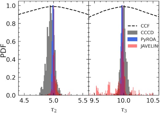
This method consistently finds smaller uncertainties than the ICCF (Yu et al. 2020); however, it does not account for poorly estimated errors on the flux measurements of AGN light curves, making it sensitive to this effect. We applied both of these methods to the three mock data sets discussed previously. For the first data set, the ICCF finds significantly larger uncertainties than our method whereas javelin on average finds slightly smaller uncertainties. These are shown in Table 1 and the posterior probability distributions are compared to our method in the right-hand panels of Fig. 2. One reason for javelin finding smaller uncertainties may be that it assumes the error bars on the flux data are accurate whereas our method expands these to account for poorly estimated errors. To investigate this further, we fit the model again but with error bars on the flux measurements that were deliberately underestimated by a factor of 5 (Case D). The resulting probability distributions for the time delays are shown in Fig. 6, comparing our method to the cross-correlation and javelin. The best-fitting parameters are shown in table 1. Our method measured consistent delays as previously found whereas javelin had some difficulties due to overfitting the noise. While the first delay was measured successfully by javelin, finding |$\tau _2 = 5.006^{+0.036}_{-0.012}$|⁠, its errors were larger and asymmetrical. The second delay had similar problems, with a measurement of |$\tau _3 = 9.975^{+0.012}_{-0.24}$|⁠, where several smaller peaks in the probability distribution skewed the lower error estimated, resulting in very uneven error bars. The cross-correlation is similar here to our method, successfully recovering the delays similar to before with similarly large uncertainties. This shows the importance of including a noise model when there is no prior knowledge that the flux measurement errors are accurately known.

Figure 6.

Posterior probability distributions of the time delays between the high S/N mock light curves but where the flux errors are deliberately underestimated by a factor of 5. The cross-correlation centroid distribution is shown in grey, our method is shown in blue and javelin is shown in red. The dashed line shows the cross-correlation function.

Open in new tab Download slide

We find that the extra error parameters increase by larger than the amount it was deliberately underestimated. This is similar to what we found when the uncertainties were not underestimated, that the algorithm is over cautious, sacrificing the very fastest variations as noise. This makes it robust when dealing with data such as this test case, where the flux errors are underestimated, and can still recover an accurate time delay. This is tested more thoroughly in Section 3.2. We also note that the error bars were not expanded as much for light curve 2 than the case where the uncertainties were not underestimated. We suspect this is due to the scatter in the size of the flux error bars across light curve 2 due to the uniform random number we added when generating the data, as described in Section 3. This scatter was larger for light curve 2 and therefore the extra variance added to the whole light curve by the algorithm is higher to make the data consistent with the other light curves when calculating the ROA. In the underestimated case, the division by a factor of 5 reduces the strength of this scatter and therefore the flux errors are not expanded as much to be consistent.

For the second data set, shown in Fig. 4, the large gaps proved difficult for the ICCF, causing both delays to be massively underestimated. This is likely due to the linear interpolation across the gaps that are being treated as a feature in the light curve when measuring the cross-correlation function. This is a known problem with the ICCF. In comparison, our method was successful in recovering the true delays as was javelin. In this case, our method produced uncertainties comparable to javelin.

The third data set contained few points, with a lower S/N of ∼ 2. Our method is consistent with ICCF and javelin and finds uncertainties comparable to javelin. Interestingly, the uncertainty in the delays from the ICCF are closer to our method and javeln than in the high S/N case.

The final data set was where the second and third light curves were blurred by a different amount. Comparing to ICCF and javelin, we see a similar result to the previous case, where the ICCF errors are the largest and pyroa is reasonably similar to javelin in its error estimates.

3.2 Verifying the accuracy of the error bars

To ensure that the errors in the time delays are being predicted accurately, 50 additional mock data sets were fitted where each of these data sets were based on a different random walk. We tested the robustness of the errors by calculating the normalized residuals of the time delay parameters with respect to the true value. This was calculated by subtracting the true value from the measured value and dividing by the average of the errors. This creates a distribution that should have a mean of 0 and a standard deviation of 1 for properly estimated error bars. As there are two time delay parameters per data set, there is a total of 100 samples. The resulting probability distributions and cumulative distributions for all 100 samples are shown in the top panel of Fig. 7.

Figure 7.

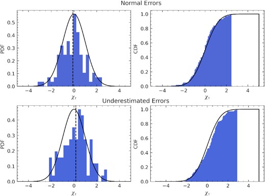
Results of the error bar testing for the time delay parameters. The top panel shows the results for normal flux errors, whereas the bottom panel shown the testing where the flux errors were deliberately underestimated by a factor of 5. Left-hand panel: probability distribution of the normalized residuals of the pairs of time delay parameters for 50 random walk light curves, relative to the true value (blue), with a Gaussian distribution with a mean of 0 and standard deviation of 1 in black. The black dashed line shows a sample mean of −0.09 in the top panel and a sample mean of 0.16 in the bottom panel. Right-hand panel: cumulative distribution of the normalized residuals (blue) compared to the Gaussian (black).

Open in new tab Download slide

This distribution has a sample mean of −0.09 ± 0.11 and a sample standard deviation of 1.06 ± 0.16, which is consistent with the expected result for well defined error bars. A mean close to 0 suggests no systematic bias in the method while a variance of 1 suggests the error bars are accurately estimated. Furthermore, we performed a Kolmogorov–Smirnov (K-S) test (Karson 1968), which tests whether the distribution of our samples is drawn from an underlying Gaussian distribution that has a mean of 0 and variance of 1. This is the null-hypothesis – that both distributions are the same – which typically requires a p-value <0.05 to reject.We use the one-sample KS test from the scipy.stats package. This calculates a p-value based on the maximum distance between the measured cumulative distribution function (CDF) and the expected normal CDF as well as the sample size. We find a p-value of 0.67, which suggests that our samples are consistent with the expected normal distribution. These tests confirm that our method is producing accurate error bars.

As discussed in Section 3.1, a major advantage of pyroa is the inclusion of a noise model that can account for underestimated flux errors. To verify that the true time delays can be recovered consistently by pyroa in this case, we repeated the previous test, fitting to 50 mock data sets but this time where the flux errors are underestimated by a factor of 5. We again calculated the normalized residuals of the time delay parameters that are plotted in the bottom panel of Fig. 7. We find a sample mean of 0.16 ± 0.11 and a sample standard deviation of 1.12 ± 0.18. The standard deviation is consistent with 1, suggesting that the size of the error bars are accurate however the mean is >1σ from zero, although it is close at 1.45σ. A KS test returns a p-value of 0.06, which is greater than the rejection criterion of >0.05, and therefore provides weak evidence that our samples are drawn from a normal distribution. The low p-value is driven largely by the mean and so shifting the distribution by the mean finds a p-value of 0.7, which is strongly consistent with a normal distribution. We suspect that the mean of 0.16 ± 0.11 is due to a lack of samples and not a systematic bias as it is only 1.45σ from the true value. This would suggest that pyroa is able to obtain accurate time delays where the flux errors are underestimated by a factor of 5, albeit with weaker evidence than the normal flux error case.

3.3 Choice of window function

For all of the testing so far, a Gaussian window function has been used. As many choices are possible, we tested the effect this has on the results of fitting the model to mock data. We used two light curves that included large gaps as the window function has a large effect on the error envelope calculated from equation (2). Fig. 8 shows the calculation of the driving light curve using three different window functions, Gaussian, inverse-cosh, and Lorentzian, given by equations (4), (5), and (6), respectively. The right-hand panel of this figure shows the resulting posterior distributions for the time delay between the two light curves.

Figure 8.

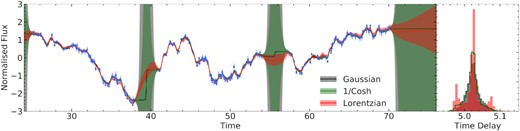
Calculation of the running optimal average at the stacking stage of the fitting procedure (Section 2.3), when fitting two light curves that contain large gaps. Three different window functions were used: a Gaussian shown in black, inverse-cosh shown in green and a Lorentzian in red. The error envelopes are shown as the shaded colour. The right-hand panel shows the probability distribution for the time delay between the light curves for each of the window functions.

Open in new tab Download slide

The main difference between them is how the error envelope behaves when there is a lack of data. The error envelope of the Gaussian window function rapidly increases in the gap whereas the error of the inverse-cosh increases slower but still becomes very large in the gaps. This is largely due to the wider wings of the inverse-cosh function compared to the Gaussian, which will allow data points far from centre of the window to still slightly contribute to the running optimal average. This effect is even more pronounced when using a Lorentzian window function, which has even wider wings. Here the error envelope only increases slightly within the gaps and increasing slower of the ends of the data. At the other extreme, a boxcar function drops to zero outwith the window, which would result in an error envelope becoming infinity within these gaps.

The probability distributions of the time delays are of similar width and peak for each window function; however, the Lorentzian shows an unusual feature, where there are two smaller peaks to each side of the main peak. The physical cause of this is unknown and as there is no real difference in the probability distributions for the Gaussian and inverse-cosh functions, we continue using a Gaussian window function for the remainder of this paper.

4 GRAVITATIONAL LENSING TIME DELAYS

In order to test this method with real data, we applied it to quasars that are gravitationally lensed by an intermediate object such as a galaxy or galaxy cluster. The lens causes the light from the quasar to form multiple images of itself on the sky. As the light from the quasar travels along vastly different paths to form each image, a time delay is induced, due to the geometric difference in the path-length that the light travels along (Cooke & Kantowski 1975), and the different gravitational potentials that the photons experience (Shapiro 1964). As the lensed quasar is variable, obtaining light curves for each of these images allows the time delay between images to be measured, using the method outlined in this paper. There are also microlensing effects taking place, which causes the brightness of the image to vary slowly with time due to objects in the lens moving relative to the source and observer (Refsdal 1964). These effects can also be modelled by including a slow varying component to the model, which modulates the brightness of each image relative to some reference image. Accounting for these effects are important for obtaining accurate delay measurements as they can create extraneous features in the light curves, resulting in poorly estimated delays.

We used public data from the COSmological MOnitoring of GRAvItational Lenses (COSMOGRAIL) project (Eigenbrod et al. 2005, and references therein), to measure the time delays between gravitationally lensed images of 34 different quasars and model microlensing effects. This requires a slightly different model than previously used, specifically to model the microlensing effects. We model the flux of each image, indexed i, where i = 1 is the image that the magnifications are measured relative to. Therefore, the model flux is given by

$$\begin{eqnarray*} f_{i}(t)= \left. \left\lbrace \begin{array}{@{}l@{\quad }l@{}}A_{1}X\left(t \right) + B_{1} & i=1 \\ \left[ A_{1}X\left(t -\tau _i \right) + B_{1} \right] 10^{-0.4 P_i(t)} & i\gt 1 \\ \end{array}\right. \right\rbrace \ , \end{eqnarray*}$$

(14)

where A₁ represents the rms flux of the reference image, B₁ represents the mean flux of the reference image, τ_i represents the time delay of image i relative to the first image, and X(t) is the driving light curve, normalized such that |$\langle$|X|$\rangle$|_t = 0, |$\langle$|X²|$\rangle$|_t = 1. The magnitude different due to microlensing is given by a fourth-order polynomial, P_i(t). This is given by

$$\begin{eqnarray*} P_i(t) = \sum _{j=0}^{4} P_{i, j}\, \eta ^j(t), \end{eqnarray*}$$

(15)

where the argument, η(t), is time normalized such that it runs between −1 and 1 over the range of the data. This is calculated by

$$\begin{eqnarray*} \eta (t) = \frac{2\left(t - t_0\right)}{\Delta t}, \end{eqnarray*}$$

(16)

where t₀ is the mid-point time of the data and Δt is the length of time between the start of observing and the end. Normalizing the time in this manner ensures that the ‘pivot point’ of the polynomial is at the centre of the data.

As we model the flux of the light curves, the data were converted from magnitudes into arbitrary flux units before modelling. This was done using

$$\begin{eqnarray*} f(t) = 3.0128 \times 10^{-5} 10^{-0.4 m(t)}, \end{eqnarray*}$$

(17)

where m(t) is the magnitude of the image as a function of time, t. This conversion gives the flux in arbitrary units with magnitudes on the order of unity for the majority of the COSMOGRAIL data. For DES 2325−5229, HE 0047−1756, PDJ 1606−233, SDSS J1515+1511, and WG 0214−2105, this factor was 3.0128 × 10⁷, as the data here measured magnitude relative to some other arbitrary value. As the parameters A₁ and B₁ have flux units, ensuring that they are not a drastically different order of magnitude (e.g. 14 orders different) to the other parameters helps when initializing the walkers to keep them linearly independent.

The method used by COSMOGRAIL measures delays between every image rather than to a single reference image (Tewes et al. 2013). Therefore, to be directly comparable, we fit our model numerous times where the time delays are measured relative to a different image each time, e.g. if there are three images (A, B, C), the model is fitted firstly with image A as the reference and then with image B as the reference. This allows all the inter-image delays to be obtained as well as the relative microlensing between all the images.

We used uniform priors between sensible limits for all the parameters and used 15 000 samples discarding the first 10 000 as burn-in for the two light-curve data. For objects with three/four light curves, we used 20 000 samples with 15 000 as burn-in. For the HE 0435−1223, we used 35 000 samples and a burn-in of 30 000 as the extra parameters required a long burn-in in this case. The number of walkers for each is ⪆ twice the number of sampled parameters. Specifically this is 7N_l + 3, where there are N_l light curves, although this number was chosen fairly arbitrary meeting the only requirement of being > twice the number of sampled parameters. Here we also include the noise model where there is extra variance added to the flux errors of each light curve as described previously.

4.1 Results

We show our results for the publicly available COSMOGRAIL light curves in Table 3. As our method measures the time delay in the opposite direction, we take the negative of the measured time delay posterior distributions in order to compare directly with COSMOGRAIL i.e. τ_AB = −τ₂, where i = 1 and 2 represent images A and B, respectively, using equation (14). The table also shows the coefficients of the fourth-order polynomial used to model the microlensing variability. The zeroth-order coefficient is of particular interest as this provides the mean difference in magnitude between the images. The higher order terms describe how the magnitude varies with time around this mean.

Table 3.

Open in new tab

COSMOGRAIL quasars.

Object	Images	Time delays (d)		Microlensing coeff. (mag)							Ref.
		This work	COSMOGRAIL	P_{i, 0}	P_{i, 1}	P_{i, 2}	P_{i, 3}	P_{i, 4}	P_{i, 5}	P_{i, 6}
2M 1134−2103	AB	\|$-29.53^{+0.63}_{-0.59}$\|	−30.5 ± 2.2	\|$0.038\,35^{+0.000\,47}_{-0.000\,44}$\|	\|$-0.0027^{+0.0013}_{-0.0012}$\|	\|$-0.0107^{+0.0035}_{-0.0035}$\|	\|$0.0259^{+0.0030}_{-0.0030}$\|	\|$-0.0009^{+0.0046}_{-0.0049}$\|	–	–	Millon et al. (2020b)
	AC	\|$8.78^{+0.56}_{-0.56}$\|	8.6 ± 1.4	\|$0.065\,02^{+0.000\,39}_{-0.000\,39}$\|	\|$0.0021^{+0.0011}_{-0.0011}$\|	\|$-0.0015^{+0.0027}_{-0.0027}$\|	\|$0.0003^{+0.0018}_{-0.0017}$\|	\|$0.0033^{+0.0031}_{-0.0032}$\|	–	–
	AD	\|$-65.6^{+2.6}_{-2.3}$\|	−71.9 ± 6.7	\|$1.7559^{+0.0011}_{-0.0011}$\|	\|$-0.0110^{+0.0064}_{-0.0058}$\|	\|$0.0151^{+0.0083}_{-0.0084}$\|	\|$0.038^{+0.015}_{-0.016}$\|	\|$-0.028^{+0.015}_{-0.014}$\|	–	–
	BC	\|$38.60^{+0.49}_{-0.50}$\|	38.9 ± 2.2	\|$0.027\,91^{+0.000\,43}_{-0.000\,42}$\|	\|$0.0005^{+0.0019}_{-0.0019}$\|	\|$-0.0202^{+0.0030}_{-0.0030}$\|	\|$-0.0156^{+0.0056}_{-0.0056}$\|	\|$0.0137^{+0.0056}_{-0.0058}$\|	–	–
	BD	\|$-36.4^{+1.9}_{-2.0}$\|	−41.5 ± 7.6	\|$1.7186^{+0.0011}_{-0.0011}$\|	\|$-0.0288^{+0.0065}_{-0.0066}$\|	\|$0.0592^{+0.0077}_{-0.0078}$\|	\|$0.028^{+0.014}_{-0.013}$\|	\|$-0.048^{+0.013}_{-0.013}$\|	–	–
	CD	\|$-75.6^{+2.4}_{-2.2}$\|	−80.5 ± 6.8	\|$1.6927^{+0.0011}_{-0.0011}$\|	\|$-0.0153^{+0.0057}_{-0.0056}$\|	\|$0.0092^{+0.0096}_{-0.0096}$\|	\|$0.059^{+0.016}_{-0.018}$\|	\|$-0.040^{+0.015}_{-0.015}$\|	–	–
DES J0407−5006	AB	\|$-123.9^{+1.5}_{-1.5}$\|	−128.4 ± 3.6	\|$1.2479^{+0.0016}_{-0.0016}$\|	\|$-0.070^{+0.014}_{-0.013}$\|	\|$0.126^{+0.023}_{-0.024}$\|	\|$-0.010^{+0.012}_{-0.012}$\|	\|$-0.051^{+0.016}_{-0.016}$\|	–	–	Millon et al. (2020b)
DES J0408−5354	AB	\|$-113.77^{+0.79}_{-0.76}$\|	−112.1 ± 2.1	\|$-0.6047^{+0.0054}_{-0.0059}$\|	\|$-0.012^{+0.036}_{-0.036}$\|	\|$-0.072^{+0.054}_{-0.052}$\|	\|$0.008^{+0.042}_{-0.041}$\|	\|$0.042^{+0.041}_{-0.048}$\|	–	–	Courbin et al. (2018)
	AD	\|$-159.1^{+1.8}_{-1.7}$\|	−155.5 ± 12.8	\|$0.511^{+0.020}_{-0.021}$\|	\|$-0.017^{+0.065}_{-0.066}$\|	\|$-0.134^{+0.072}_{-0.068}$\|	\|$-0.017^{+0.094}_{-0.010}$\|	\|$0.186^{+0.074}_{-0.067}$\|	–	–
	BD	\|$-47.6^{+1.3}_{-1.4}$\|	−42.4 ± 17.6	\|$1.1244^{+0.0043}_{-0.0039}$\|	\|$-0.0643^{+0.0092}_{-0.0087}$\|	\|$-0.096^{+0.027}_{-0.029}$\|	\|$0.111^{+0.023}_{-0.022}$\|	\|$0.077^{+0.031}_{-0.031}$\|	–	–
DES 2325−5229	AB	\|$44.83^{+0.90}_{-0.87}$\|	43.9 ± 4.2	\|$1.0985^{+0.0040}_{-0.0041}$\|	\|$-0.131^{+0.011}_{-0.011}$\|	\|$0.045^{+0.037}_{-0.037}$\|	\|$0.397^{+0.033}_{-0.032}$\|	\|$0.037^{+0.050}_{-0.049}$\|	–	–	Millon et al. (2020b)
HE 0047−1756	AB	\|$-11.00^{+0.39}_{-0.39}$\|	−10.8 ± 1.0	\|$1.6127^{+0.0014}_{-0.0013}$\|	\|$-0.0140^{+0.0029}_{-0.0029}$\|	\|$0.0617^{+0.0060}_{-0.0064}$\|	\|$0.0235^{+0.0040}_{-0.0040}$\|	\|$-0.0550^{+0.0066}_{-0.0063}$\|	–	–	Millon et al. (2020b)
HE 0230−2130	AC	\|$17.7^{+2.1}_{-2.1}$\|	15.7 ± 3.9	\|$1.5081^{+0.0070}_{-0.0068}$\|	\|$-0.129^{+0.013}_{-0.013}$\|	\|$0.202^{+0.047}_{-0.047}$\|	\|$-0.002^{+0.017}_{-0.018}$\|	\|$-0.139^{+0.049}_{-0.051}$\|	–	–	Millon et al. (2020a)
	AD	\|$-10.5^{+9.8}_{-6.1}$\|	–	\|$2.321^{+0.014}_{-0.016}$\|	\|$-0.107^{+0.024}_{-0.024}$\|	\|$0.183^{+0.089}_{-0.086}$\|	\|$-0.098^{+0.032}_{-0.031}$\|	\|$-0.226^{+0.089}_{-0.092}$\|	–	–
	CD	\|$-26.9^{+11.4}_{-7.1}$\|	–	\|$0.802^{+0.014}_{-0.015}$\|	\|$0.035^{+0.029}_{-0.029}$\|	\|$0.004^{+0.010}_{-0.093}$\|	\|$-0.111^{+0.039}_{-0.039}$\|	\|$-0.11^{+0.10}_{-0.10}$\|	–	–
HE 0435−1223	AB	\|$-8.00^{+0.37}_{-0.36}$\|	−9.0 ± 0.8	\|$0.2555^{+0.0019}_{-0.0019}$\|	\|$-0.4259^{+0.0073}_{-0.0068}$\|	\|$0.887^{+0.021}_{-0.021}$\|	\|$0.793^{+0.024}_{-0.025}$\|	\|$-1.910^{+0.056}_{-0.055}$\|	\|$0.546^{+0.020}_{-0.020}$\|	\|$0.932^{+0.038}_{-0.039}$\|	Millon et al. (2020a)
	AC	\|$-0.12^{+0.26}_{-0.20}$\|	−0.8 ± 0.7	\|$0.6614^{+0.0017}_{-0.0017}$\|	\|$-0.4137^{+0.0068}_{-0.0068}$\|	\|$0.773^{+0.020}_{-0.019}$\|	\|$0.497^{+0.023}_{-0.023}$\|	\|$-1.438^{+0.049}_{-0.052}$\|	\|$-0.218^{+0.018}_{-0.019}$\|	\|$0.674^{+0.036}_{-0.033}$\|
	AD	\|$-13.99^{+0.19}_{-0.27}$\|	−13.8 ± 0.8	\|$1.2895^{+0.0019}_{-0.0020}$\|	\|$-0.1620^{+0.0074}_{-0.0074}$\|	\|$0.781^{+0.022}_{-0.022}$\|	\|$0.369^{+0.026}_{-0.025}$\|	\|$-1.678^{+0.059}_{-0.060}$\|	\|$-0.202^{+0.020}_{-0.021}$\|	\|$0.902^{+0.041}_{-0.041}$\|
	BC	\|$9.06^{+0.20}_{-0.28}$\|	7.8 ± 0.9	\|$0.4069^{+0.0018}_{-0.0018}$\|	\|$0.0076^{+0.0051}_{-0.0054}$\|	\|$-0.121^{+0.019}_{-0.019}$\|	\|$-0.275^{+0.019}_{-0.018}$\|	\|$0.480^{+0.049}_{-0.049}$\|	\|$0.314^{+0.016}_{-0.016}$\|	\|$-0.257^{+0.033}_{-0.034}$\|
	BD	\|$-5.22^{+0.39}_{-0.41}$\|	−5.4 ± 0.8	\|$1.0326^{+0.0020}_{-0.0020}$\|	\|$0.2693^{+0.0059}_{-0.0061}$\|	\|$-0.101^{+0.022}_{-0.023}$\|	\|$-0.448^{+0.021}_{-0.021}$\|	\|$0.228^{+0.058}_{-0.056}$\|	\|$0.363^{+0.018}_{-0.018}$\|	\|$-0.032^{+0.039}_{-0.040}$\|
	CD	\|$-13.99^{+0.19}_{-0.30}$\|	−13.2 ± 0.8	\|$0.6254^{+0.0019}_{-0.0019}$\|	\|$0.2609^{+0.0057}_{-0.0057}$\|	\|$0.017^{+0.020}_{-0.020}$\|	\|$-0.163^{+0.020}_{-0.021}$\|	\|$-0.247^{+0.050}_{-0.051}$\|	\|$0.041^{+0.018}_{-0.017}$\|	\|$0.229^{+0.036}_{-0.035}$\|
HE 2149−2745	AB	\|$-71.3^{+3.3}_{-3.4}$\|	−39.0 ± 15.8	\|$1.4350^{+0.0018}_{-0.0018}$\|	\|$-0.0390^{+0.0050}_{-0.0050}$\|	\|$-0.184^{+0.014}_{-0.013}$\|	\|$-0.1197^{+0.0078}_{-0.0081}$\|	\|$0.175^{+0.015}_{-0.016}$\|	–	–	Millon et al. (2020a)
HS 0818+1227	AB	\|$-39.8^{+3.3}_{-3.2}$\|	−153.8 ± 13.9	\|$1.9478^{+0.0040}_{-0.0041}$\|	\|$0.1287^{+0.0081}_{-0.0080}$\|	\|$0.102^{+0.023}_{-0.023}$\|	\|$-0.038^{+0.011}_{-0.011}$\|	\|$-0.116^{+0.023}_{-0.024}$\|	–	–	Millon et al. (2020a)
HS 2209+1914	AB	\|$24.0^{+2.4}_{-2.4}$\|	20.0 ± 5.0	\|$0.216\,99^{+0.0000\,53}_{-0.000\,55}$\|	\|$0.0196^{+0.0030}_{-0.0029}$\|	\|$-0.0071^{+0.0064}_{-0.0066}$\|	\|$0.0870^{+0.0059}_{-0.0059}$\|	\|$0.0707^{+0.0092}_{-0.0091}$\|	–	–	Eulaers et al. (2013)
Q J0158−4325	AB	\|$-34.9^{+3.2}_{-3.0}$\|	−22.7 ± 3.6	\|$1.1236^{+0.0031}_{-0.0031}$\|	\|$0.6289^{+0.0071}_{-0.0072}$\|	\|$-0.148^{+0.020}_{-0.020}$\|	\|$-0.075^{+0.011}_{-0.010}$\|	\|$-0.027^{+0.022}_{-0.022}$\|	–	–	Millon et al. (2020a)
SDSS J0246−0825	AB	\|$3.1^{+2.0}_{-2.0}$\|	0.8 ± 5.1	\|$1.8400^{+0.0051}_{-0.0050}$\|	\|$0.476^{+0.013}_{-0.013}$\|	\|$-0.892^{+0.035}_{-0.034}$\|	\|$-0.314^{+0.020}_{-0.020}$\|	\|$0.673^{+0.037}_{-0.038}$\|	–	–	Millon et al. (2020a)
SDSS J0832+0404	AB	\|$-136.5^{+1.8}_{-1.9}$\|	−125.3 ± 18.1	\|$0.9912^{+0.0064}_{-0.0066}$\|	\|$-0.066^{+0.018}_{-0.019}$\|	\|$-0.009^{+0.042}_{-0.043}$\|	\|$-0.416^{+0.026}_{-0.024}$\|	\|$0.346^{+0.048}_{-0.047}$\|	–	–	Millon et al. (2020a)
SDSS J0924+0219	AB	\|$0.6^{+2.7}_{-2.6}$\|	2.4 ± 3.8	\|$1.3827^{+0.0055}_{-0.0056}$\|	\|$-0.014^{+0.015}_{-0.015}$\|	\|$0.291^{+0.038}_{-0.039}$\|	\|$0.476^{+0.023}_{-0.024}$\|	\|$-0.693^{+0.046}_{-0.047}$\|	–	–	Millon et al. (2020a)
	AC	\|$-30.9^{+7.9}_{-8.0}$\|	–	\|$2.785^{+0.017}_{-0.017}$\|	\|$0.082^{+0.047}_{-0.045}$\|	\|$0.14^{+0.11}_{-0.11}$\|	\|$0.827^{+0.081}_{-0.077}$\|	\|$-0.54^{+0.14}_{-0.13}$\|	–	–
	BC	\|$-32.5^{+8.4}_{-8.5}$\|	–	\|$1.401^{+0.018}_{-0.018}$\|	\|$0.099^{+0.049}_{-0.046}$\|	\|$-0.13^{+0.12}_{-0.12}$\|	\|$0.325^{+0.081}_{-0.083}$\|	\|$0.16^{+0.15}_{-0.14}$\|	–	–
SDSS J1001+5027	AB	\|$-119.9^{+1.4}_{-1.5}$\|	−119.3 ± 3.3	\|$0.420\,39^{+0.000\,10}_{-0.000\,93}$\|	\|$0.0004^{+0.0039}_{-0.000\,41}$\|	\|$0.0069^{+0.0089}_{-0.000\,91}$\|	\|$-0.0215^{+0.0081}_{-0.0080}$\|	\|$-0.024^{+0.014}_{-0.013}$\|	–	–	Rathna Kumar et al. (2013)
SDSS J1206+4332	AB	\|$-113.0^{+1.1}_{-1.2}$\|	−111.3 ± 3.0	\|$0.3332^{+0.0023}_{-0.0022}$\|	\|$-0.1670^{+0.0075}_{-0.0073}$\|	\|$-0.213^{+0.016}_{-0.016}$\|	\|$0.104^{+0.015}_{-0.015}$\|	\|$0.141^{+0.023}_{-0.023}$\|	–	–	Eulaers et al. (2013)
SDSS J1226−0006	AB	\|$25.63^{+0.89}_{-0.76}$\|	–	\|$0.9113^{+0.0025}_{-0.0024}$\|	\|$0.2639^{+0.0055}_{-0.0056}$\|	\|$0.160^{+0.016}_{-0.016}$\|	\|$-0.1019^{+0.0079}_{-0.0080}$\|	\|$-0.082^{+0.017}_{-0.017}$\|	–	–	Millon et al. (2020a)
SDSS J1320+1644	AB	\|$-157.1^{+14.2}_{-14.9}$\|	–	\|$0.894^{+0.031}_{-0.028}$\|	\|$0.178^{+0.053}_{-0.066}$\|	\|$-0.24^{+0.24}_{-0.39}$\|	\|$-0.025^{+0.066}_{-0.070}$\|	\|$0.04^{+0.28}_{-0.19}$\|	–	–	Millon et al. (2020a)
SDSS J1322+1052	AB	\|$105.6^{+10.0}_{-11.5}$\|	–	\|$1.6613^{+0.0068}_{-0.0070}$\|	\|$-0.077^{+0.023}_{-0.024}$\|	\|$-0.474^{+0.053}_{-0.053}$\|	\|$0.223^{+0.040}_{-0.039}$\|	\|$0.581^{+0.063}_{-0.065}$\|	–	–	Millon et al. (2020a)
SDSS J1335+0118	AB	\|$-59.0^{+4.1}_{-4.2}$\|	−56.0 ± 5.9	\|$1.0958^{+0.0020}_{-0.0021}$\|	\|$-0.1001^{+0.0046}_{-0.0046}$\|	\|$-0.038^{+0.013}_{-0.013}$\|	\|$0.0144^{+0.0065}_{-0.0072}$\|	\|$0.051^{+0.014}_{-0.014}$\|	–	–	Millon et al. (2020a)
SDSS J1349+1227	AB	\|$-140.8^{+7.5}_{-6.5}$\|	–	\|$1.3180^{+0.0056}_{-0.0069}$\|	\|$-0.007^{+0.013}_{-0.012}$\|	\|$0.020^{+0.039}_{-0.036}$\|	\|$0.089^{+0.018}_{-0.018}$\|	\|$0.005^{+0.039}_{-0.041}$\|	–	–	Millon et al. (2020a)
SDSS J1405+0959	AB	\|$-82.8^{+12.3}_{-19.7}$\|	–	\|$0.778^{+0.011}_{-0.010}$\|	\|$0.019^{+0.024}_{-0.024}$\|	\|$0.023^{+0.060}_{-0.061}$\|	\|$-0.004^{+0.033}_{-0.034}$\|	\|$0.035^{+0.069}_{-0.069}$\|	–	–	Millon et al. (2020a)
SDSS J1455+1447	AB	\|$-43.4^{+2.3}_{-2.2}$\|	−47.2 ± 7.6	\|$1.0711^{+0.0041}_{-0.0039}$\|	\|$0.0426^{+0.0084}_{-0.0088}$\|	\|$0.002^{+0.026}_{-0.026}$\|	\|$0.007^{+0.012}_{-0.012}$\|	\|$0.024^{+0.027}_{-0.028}$\|	–	–	Millon et al. (2020a)
SDSS J1515+1511	AB	\|$-208.3^{+1.8}_{-1.8}$\|	−210.2 ± 5.6	\|$0.3679^{+0.0022}_{-0.0024}$\|	\|$0.0117^{+0.0070}_{-0.0067}$\|	\|$-0.027^{+0.021}_{-0.019}$\|	\|$-0.025^{+0.019}_{-0.019}$\|	\|$0.053^{+0.032}_{-0.035}$\|	–	–	Millon et al. (2020a)
SDSS J1620+1203	AB	\|$-158.3^{+2.4}_{-2.5}$\|	−171.5 ± 8.7	\|$1.2387^{+0.0064}_{-0.0067}$\|	\|$0.003^{+0.016}_{-0.016}$\|	\|$-0.082^{+0.048}_{-0.045}$\|	\|$-0.093^{+0.037}_{-0.036}$\|	\|$0.148^{+0.061}_{-0.062}$\|	–	–	Millon et al. (2020a)
PG 1115+080	AB	\|$-6.90^{+0.68}_{-0.69}$\|	−8.3 ± 1.5	\|$2.5709^{+0.0018}_{-0.0018}$\|	\|$0.0211^{+0.0041}_{-0.0041}$\|	\|$0.037^{+0.012}_{-0.012}$\|	\|$-0.0103^{+0.0060}_{-0.0059}$\|	\|$-0.034^{+0.013}_{-0.012}$\|	–	–	Bonvin et al. (2018)
	AC	\|$9.43^{+0.83}_{-0.82}$\|	9.9 ± 1.1	\|$2.2193^{+0.0017}_{-0.0016}$\|	\|$0.0040^{+0.0035}_{-0.0035}$\|	\|$0.033^{+0.010}_{-0.010}$\|	\|$-0.0048^{+0.0066}_{-0.0063}$\|	\|$-0.038^{+0.012}_{-0.012}$\|	–	–
	BC	\|$-16.35^{+0.94}_{-0.90}$\|	18.8 ± 1.6	\|$-0.3569^{+0.0022}_{-0.0023}$\|	\|$-0.0268^{+0.0053}_{-0.0051}$\|	\|$0.012^{+0.012}_{-0.011}$\|	\|$0.0255^{+0.0098}_{-0.0099}$\|	\|$-0.009^{+0.014}_{-0.014}$\|	–	–
PSJ 1606−2333	AB	\|$-12.9^{+1.1}_{-1.1}$\|	−10.4 ± 2.2	\|$0.1523^{+0.0029}_{-0.0030}$\|	\|$0.0342^{+0.0046}_{-0.0048}$\|	\|$0.001^{+0.012}_{-0.011}$\|	\|$-0.0186^{+0.0074}_{-0.0074}$\|	\|$-0.011^{+0.012}_{-0.013}$\|	–	–	Millon et al. (2020b)
	AC	\|$-30.6^{+2.2}_{-2.4}$\|	−29.2 ± 4.7	\|$0.5593^{+0.0059}_{-0.0060}$\|	\|$0.0338^{+0.0050}_{-0.0053}$\|	\|$-0.056^{+0.022}_{-0.023}$\|	\|$0.001^{+0.010}_{-0.010}$\|	\|$0.003^{+0.023}_{-0.023}$\|	–	–
	AD	\|$-40.1^{+2.8}_{-2.4}$\|	−45.7 ± 10.9	\|$0.7449^{+0.0071}_{-0.0069}$\|	\|$0.0689^{+0.0066}_{-0.0064}$\|	\|$-0.037^{+0.025}_{-0.025}$\|	\|$-0.004^{+0.014}_{-0.014}$\|	\|$-0.022^{+0.024}_{-0.024}$\|	–	–
	BC	\|$-17.5^{+1.8}_{-2.0}$\|	−19.3 ± 4.5	\|$0.4114^{+0.0045}_{-0.0049}$\|	\|$-0.0011^{+0.0054}_{-0.0054}$\|	\|$-0.056^{+0.021}_{-0.020}$\|	\|$0.0161^{+0.0090}_{-0.0091}$\|	\|$0.005^{+0.020}_{-0.021}$\|	–	–
	BD	\|$-27.4^{+3.2}_{-2.7}$\|	−36.2 ± 10.4	\|$0.5986^{+0.0064}_{-0.0061}$\|	\|$0.0349^{+0.0064}_{-0.0066}$\|	\|$-0.038^{+0.024}_{-0.027}$\|	\|$0.0119^{+0.013}_{-0.012}$\|	\|$-0.023^{+0.025}_{-0.024}$\|	–	–
	CD	\|$-9.0^{+3.9}_{-3.4}$\|	−13.8 ± 8.4	\|$0.1874^{+0.0084}_{-0.0073}$\|	\|$0.0262^{+0.0066}_{-0.0075}$\|	\|$0.034^{+0.028}_{-0.032}$\|	\|$0.002^{+0.011}_{-0.010}$\|	\|$-0.047^{+0.026}_{-0.025}$\|	–	–
Q 1355−2257	AB	\|$-64.5^{+4.6}_{-4.7}$\|	−81.5 ± 11.4	\|$1.5528^{+0.0049}_{-0.0049}$\|	\|$-0.120^{+0.015}_{-0.015}$\|	\|$0.287^{+0.039}_{-0.039}$\|	\|$0.005^{+0.037}_{-0.037}$\|	\|$-0.259^{+0.059}_{-0.058}$\|	–	–	Millon et al. (2020a)
Q 2237+0305	AB	\|$11.7^{+4.7}_{-5.4}$\|	–	\|$0.8885^{+0.0050}_{-0.0051}$\|	\|$-0.128^{+0.016}_{-0.016}$\|	\|$0.139^{+0.034}_{-0.034}$\|	\|$0.021^{+0.023}_{-0.022}$\|	\|$-0.127^{+0.037}_{-0.035}$\|	–	–	Millon et al. (2020a)
UM 673	AB	\|$7.7^{+10.6}_{-13.0}$\|	−97.7 ± 15.8	\|$2.1667^{+0.0022}_{-0.0022}$\|	\|$0.0170^{+0.0066}_{-0.0066}$\|	\|$-0.127^{+0.015}_{-0.015}$\|	\|$-0.008^{+0.010}_{-0.010}$\|	\|$0.176^{+0.016}_{-0.016}$\|	–	–	Millon et al. (2020a)
WFI J2026−4536	AB	\|$4.4^{+2.1}_{-2.3}$\|	18.0 ± 4.8	\|$1.9398^{+0.0027}_{-0.0029}$\|	\|$-0.1713^{+0.0075}_{-0.0075}$\|	\|$0.255^{+0.018}_{-0.019}$\|	\|$0.108^{+0.011}_{-0.012}$\|	\|$-0.224^{+0.021}_{-0.021}$\|	–	–	Millon et al. (2020a)
	AC	\|$2.6^{+4.2}_{-4.6}$\|	–	\|$2.0434^{+0.0050}_{-0.0050}$\|	\|$-0.031^{+0.014}_{-0.014}$\|	\|$0.246^{+0.035}_{-0.036}$\|	\|$-0.023^{+0.022}_{-0.022}$\|	\|$-0.196^{+0.041}_{-0.041}$\|	–	–
	BC	\|$2.2^{+5.1}_{-5.5}$\|	–	\|$0.1031^{+0.0056}_{-0.0055}$\|	\|$0.144^{+0.015}_{-0.016}$\|	\|$-0.006^{+0.039}_{-0.039}$\|	\|$0.137^{+0.025}_{-0.024}$\|	\|$0.025^{+0.046}_{-0.045}$\|	–	–
WFI 2033−4723	AB	\|$40.54^{+0.60}_{-0.64}$\|	36.2 ± 0.7	\|$1.0681^{+0.0013}_{-0.0012}$\|	\|$-0.0072^{+0.0030}_{-0.0030}$\|	\|$0.0349^{+0.0083}_{-0.0081}$\|	\|$0.0390^{+0.0052}_{-0.0050}$\|	\|$0.019^{+0.010}_{-0.010}$\|	–	–	Bonvin et al. (2019)
	AC	\|$-27.23^{+0.69}_{-0.66}$\|	−23.3 ± 1.3	\|$1.3830^{+0.0014}_{-0.0014}$\|	\|$0.0766^{+0.0033}_{-0.0033}$\|	\|$-0.0752^{+0.0086}_{-0.0091}$\|	\|$-0.0077^{+0.0054}_{-0.0055}$\|	\|$0.000^{+0.010}_{-0.011}$\|	–	–
	BC	\|$-68.3^{+1.2}_{-0.8}$\|	−59.4 ± 1.3	\|$0.3146^{+0.0016}_{-0.0016}$\|	\|$0.0859^{+0.0041}_{-0.0040}$\|	\|$-0.106^{+0.011}_{-0.012}$\|	\|$-0.0456^{+0.0066}_{-0.0069}$\|	\|$-0.021^{+0.014}_{-0.014}$\|	–	–
WG 0214−2105	AB	\|$10.24^{+0.67}_{-0.64}$\|	7.5 ± 2.8	\|$-0.0773^{+0.0043}_{-0.0042}$\|	\|$-0.1127^{+0.0052}_{-0.0054}$\|	\|$0.031^{+0.019}_{-0.019}$\|	\|$0.0632^{+0.0080}_{-0.0076}$\|	\|$-0.0635^{+0.0018}_{-0.0018}$\|	–	–	Millon et al. (2020b)
	AC	\|$-5.82^{+0.69}_{-0.69}$\|	−6.7 ± 3.6	\|$-0.0413^{+0.0041}_{-0.0041}$\|	\|$-0.0320^{+0.0057}_{-0.0057}$\|	\|$-0.020^{+0.019}_{-0.019}$\|	\|$0.0118^{+0.0083}_{-0.0086}$\|	\|$0.012^{+0.018}_{-0.018}$\|	–	–
	AD	\|$-43.2^{+1.8}_{-1.8}$\|	−14.1 ± 4.9	\|$0.6228^{+0.0079}_{-0.0078}$\|	\|$-0.111^{+0.013}_{-0.013}$\|	\|$0.403^{+0.036}_{-0.035}$\|	\|$0.241^{+0.023}_{-0.023}$\|	\|$-0.339^{+0.038}_{-0.039}$\|	–	–
	BC	\|$-16.01^{+0.56}_{-0.59}$\|	−14.2 ± 2.6	\|$0.0314^{+0.0043}_{-0.0043}$\|	\|$0.0840^{+0.0058}_{-0.0058}$\|	\|$-0.047^{+0.019}_{-0.019}$\|	\|$-0.0657^{+0.0093}_{-0.0090}$\|	\|$0.083^{+0.020}_{-0.019}$\|	–	–
	BD	\|$-53.5^{+1.7}_{-1.7}$\|	−21.6 ± 4.6	\|$0.6812^{+0.0079}_{-0.0078}$\|	\|$0.007^{+0.014}_{-0.014}$\|	\|$0.413^{+0.036}_{-0.037}$\|	\|$0.131^{+0.024}_{-0.024}$\|	\|$-0.271^{+0.040}_{-0.041}$\|	–	–
	CD	\|$-37.4^{+1.6}_{-1.6}$\|	−7.5 ± 4.7	\|$0.6616^{+0.0074}_{-0.0077}$\|	\|$-0.083^{+0.012}_{-0.012}$\|	\|$0.422^{+0.035}_{-0.035}$\|	\|$0.232^{+0.020}_{-0.020}$\|	\|$-0.346^{+0.037}_{-0.038}$\|	–	–

Object	Images	Time delays (d)		Microlensing coeff. (mag)							Ref.
		This work	COSMOGRAIL	P_{i, 0}	P_{i, 1}	P_{i, 2}	P_{i, 3}	P_{i, 4}	P_{i, 5}	P_{i, 6}
2M 1134−2103	AB	\|$-29.53^{+0.63}_{-0.59}$\|	−30.5 ± 2.2	\|$0.038\,35^{+0.000\,47}_{-0.000\,44}$\|	\|$-0.0027^{+0.0013}_{-0.0012}$\|	\|$-0.0107^{+0.0035}_{-0.0035}$\|	\|$0.0259^{+0.0030}_{-0.0030}$\|	\|$-0.0009^{+0.0046}_{-0.0049}$\|	–	–	Millon et al. (2020b)
	AC	\|$8.78^{+0.56}_{-0.56}$\|	8.6 ± 1.4	\|$0.065\,02^{+0.000\,39}_{-0.000\,39}$\|	\|$0.0021^{+0.0011}_{-0.0011}$\|	\|$-0.0015^{+0.0027}_{-0.0027}$\|	\|$0.0003^{+0.0018}_{-0.0017}$\|	\|$0.0033^{+0.0031}_{-0.0032}$\|	–	–
	AD	\|$-65.6^{+2.6}_{-2.3}$\|	−71.9 ± 6.7	\|$1.7559^{+0.0011}_{-0.0011}$\|	\|$-0.0110^{+0.0064}_{-0.0058}$\|	\|$0.0151^{+0.0083}_{-0.0084}$\|	\|$0.038^{+0.015}_{-0.016}$\|	\|$-0.028^{+0.015}_{-0.014}$\|	–	–
	BC	\|$38.60^{+0.49}_{-0.50}$\|	38.9 ± 2.2	\|$0.027\,91^{+0.000\,43}_{-0.000\,42}$\|	\|$0.0005^{+0.0019}_{-0.0019}$\|	\|$-0.0202^{+0.0030}_{-0.0030}$\|	\|$-0.0156^{+0.0056}_{-0.0056}$\|	\|$0.0137^{+0.0056}_{-0.0058}$\|	–	–
	BD	\|$-36.4^{+1.9}_{-2.0}$\|	−41.5 ± 7.6	\|$1.7186^{+0.0011}_{-0.0011}$\|	\|$-0.0288^{+0.0065}_{-0.0066}$\|	\|$0.0592^{+0.0077}_{-0.0078}$\|	\|$0.028^{+0.014}_{-0.013}$\|	\|$-0.048^{+0.013}_{-0.013}$\|	–	–
	CD	\|$-75.6^{+2.4}_{-2.2}$\|	−80.5 ± 6.8	\|$1.6927^{+0.0011}_{-0.0011}$\|	\|$-0.0153^{+0.0057}_{-0.0056}$\|	\|$0.0092^{+0.0096}_{-0.0096}$\|	\|$0.059^{+0.016}_{-0.018}$\|	\|$-0.040^{+0.015}_{-0.015}$\|	–	–
DES J0407−5006	AB	\|$-123.9^{+1.5}_{-1.5}$\|	−128.4 ± 3.6	\|$1.2479^{+0.0016}_{-0.0016}$\|	\|$-0.070^{+0.014}_{-0.013}$\|	\|$0.126^{+0.023}_{-0.024}$\|	\|$-0.010^{+0.012}_{-0.012}$\|	\|$-0.051^{+0.016}_{-0.016}$\|	–	–	Millon et al. (2020b)
DES J0408−5354	AB	\|$-113.77^{+0.79}_{-0.76}$\|	−112.1 ± 2.1	\|$-0.6047^{+0.0054}_{-0.0059}$\|	\|$-0.012^{+0.036}_{-0.036}$\|	\|$-0.072^{+0.054}_{-0.052}$\|	\|$0.008^{+0.042}_{-0.041}$\|	\|$0.042^{+0.041}_{-0.048}$\|	–	–	Courbin et al. (2018)
	AD	\|$-159.1^{+1.8}_{-1.7}$\|	−155.5 ± 12.8	\|$0.511^{+0.020}_{-0.021}$\|	\|$-0.017^{+0.065}_{-0.066}$\|	\|$-0.134^{+0.072}_{-0.068}$\|	\|$-0.017^{+0.094}_{-0.010}$\|	\|$0.186^{+0.074}_{-0.067}$\|	–	–
	BD	\|$-47.6^{+1.3}_{-1.4}$\|	−42.4 ± 17.6	\|$1.1244^{+0.0043}_{-0.0039}$\|	\|$-0.0643^{+0.0092}_{-0.0087}$\|	\|$-0.096^{+0.027}_{-0.029}$\|	\|$0.111^{+0.023}_{-0.022}$\|	\|$0.077^{+0.031}_{-0.031}$\|	–	–
DES 2325−5229	AB	\|$44.83^{+0.90}_{-0.87}$\|	43.9 ± 4.2	\|$1.0985^{+0.0040}_{-0.0041}$\|	\|$-0.131^{+0.011}_{-0.011}$\|	\|$0.045^{+0.037}_{-0.037}$\|	\|$0.397^{+0.033}_{-0.032}$\|	\|$0.037^{+0.050}_{-0.049}$\|	–	–	Millon et al. (2020b)
HE 0047−1756	AB	\|$-11.00^{+0.39}_{-0.39}$\|	−10.8 ± 1.0	\|$1.6127^{+0.0014}_{-0.0013}$\|	\|$-0.0140^{+0.0029}_{-0.0029}$\|	\|$0.0617^{+0.0060}_{-0.0064}$\|	\|$0.0235^{+0.0040}_{-0.0040}$\|	\|$-0.0550^{+0.0066}_{-0.0063}$\|	–	–	Millon et al. (2020b)
HE 0230−2130	AC	\|$17.7^{+2.1}_{-2.1}$\|	15.7 ± 3.9	\|$1.5081^{+0.0070}_{-0.0068}$\|	\|$-0.129^{+0.013}_{-0.013}$\|	\|$0.202^{+0.047}_{-0.047}$\|	\|$-0.002^{+0.017}_{-0.018}$\|	\|$-0.139^{+0.049}_{-0.051}$\|	–	–	Millon et al. (2020a)
	AD	\|$-10.5^{+9.8}_{-6.1}$\|	–	\|$2.321^{+0.014}_{-0.016}$\|	\|$-0.107^{+0.024}_{-0.024}$\|	\|$0.183^{+0.089}_{-0.086}$\|	\|$-0.098^{+0.032}_{-0.031}$\|	\|$-0.226^{+0.089}_{-0.092}$\|	–	–
	CD	\|$-26.9^{+11.4}_{-7.1}$\|	–	\|$0.802^{+0.014}_{-0.015}$\|	\|$0.035^{+0.029}_{-0.029}$\|	\|$0.004^{+0.010}_{-0.093}$\|	\|$-0.111^{+0.039}_{-0.039}$\|	\|$-0.11^{+0.10}_{-0.10}$\|	–	–
HE 0435−1223	AB	\|$-8.00^{+0.37}_{-0.36}$\|	−9.0 ± 0.8	\|$0.2555^{+0.0019}_{-0.0019}$\|	\|$-0.4259^{+0.0073}_{-0.0068}$\|	\|$0.887^{+0.021}_{-0.021}$\|	\|$0.793^{+0.024}_{-0.025}$\|	\|$-1.910^{+0.056}_{-0.055}$\|	\|$0.546^{+0.020}_{-0.020}$\|	\|$0.932^{+0.038}_{-0.039}$\|	Millon et al. (2020a)
	AC	\|$-0.12^{+0.26}_{-0.20}$\|	−0.8 ± 0.7	\|$0.6614^{+0.0017}_{-0.0017}$\|	\|$-0.4137^{+0.0068}_{-0.0068}$\|	\|$0.773^{+0.020}_{-0.019}$\|	\|$0.497^{+0.023}_{-0.023}$\|	\|$-1.438^{+0.049}_{-0.052}$\|	\|$-0.218^{+0.018}_{-0.019}$\|	\|$0.674^{+0.036}_{-0.033}$\|
	AD	\|$-13.99^{+0.19}_{-0.27}$\|	−13.8 ± 0.8	\|$1.2895^{+0.0019}_{-0.0020}$\|	\|$-0.1620^{+0.0074}_{-0.0074}$\|	\|$0.781^{+0.022}_{-0.022}$\|	\|$0.369^{+0.026}_{-0.025}$\|	\|$-1.678^{+0.059}_{-0.060}$\|	\|$-0.202^{+0.020}_{-0.021}$\|	\|$0.902^{+0.041}_{-0.041}$\|
	BC	\|$9.06^{+0.20}_{-0.28}$\|	7.8 ± 0.9	\|$0.4069^{+0.0018}_{-0.0018}$\|	\|$0.0076^{+0.0051}_{-0.0054}$\|	\|$-0.121^{+0.019}_{-0.019}$\|	\|$-0.275^{+0.019}_{-0.018}$\|	\|$0.480^{+0.049}_{-0.049}$\|	\|$0.314^{+0.016}_{-0.016}$\|	\|$-0.257^{+0.033}_{-0.034}$\|
	BD	\|$-5.22^{+0.39}_{-0.41}$\|	−5.4 ± 0.8	\|$1.0326^{+0.0020}_{-0.0020}$\|	\|$0.2693^{+0.0059}_{-0.0061}$\|	\|$-0.101^{+0.022}_{-0.023}$\|	\|$-0.448^{+0.021}_{-0.021}$\|	\|$0.228^{+0.058}_{-0.056}$\|	\|$0.363^{+0.018}_{-0.018}$\|	\|$-0.032^{+0.039}_{-0.040}$\|
	CD	\|$-13.99^{+0.19}_{-0.30}$\|	−13.2 ± 0.8	\|$0.6254^{+0.0019}_{-0.0019}$\|	\|$0.2609^{+0.0057}_{-0.0057}$\|	\|$0.017^{+0.020}_{-0.020}$\|	\|$-0.163^{+0.020}_{-0.021}$\|	\|$-0.247^{+0.050}_{-0.051}$\|	\|$0.041^{+0.018}_{-0.017}$\|	\|$0.229^{+0.036}_{-0.035}$\|
HE 2149−2745	AB	\|$-71.3^{+3.3}_{-3.4}$\|	−39.0 ± 15.8	\|$1.4350^{+0.0018}_{-0.0018}$\|	\|$-0.0390^{+0.0050}_{-0.0050}$\|	\|$-0.184^{+0.014}_{-0.013}$\|	\|$-0.1197^{+0.0078}_{-0.0081}$\|	\|$0.175^{+0.015}_{-0.016}$\|	–	–	Millon et al. (2020a)
HS 0818+1227	AB	\|$-39.8^{+3.3}_{-3.2}$\|	−153.8 ± 13.9	\|$1.9478^{+0.0040}_{-0.0041}$\|	\|$0.1287^{+0.0081}_{-0.0080}$\|	\|$0.102^{+0.023}_{-0.023}$\|	\|$-0.038^{+0.011}_{-0.011}$\|	\|$-0.116^{+0.023}_{-0.024}$\|	–	–	Millon et al. (2020a)
HS 2209+1914	AB	\|$24.0^{+2.4}_{-2.4}$\|	20.0 ± 5.0	\|$0.216\,99^{+0.0000\,53}_{-0.000\,55}$\|	\|$0.0196^{+0.0030}_{-0.0029}$\|	\|$-0.0071^{+0.0064}_{-0.0066}$\|	\|$0.0870^{+0.0059}_{-0.0059}$\|	\|$0.0707^{+0.0092}_{-0.0091}$\|	–	–	Eulaers et al. (2013)
Q J0158−4325	AB	\|$-34.9^{+3.2}_{-3.0}$\|	−22.7 ± 3.6	\|$1.1236^{+0.0031}_{-0.0031}$\|	\|$0.6289^{+0.0071}_{-0.0072}$\|	\|$-0.148^{+0.020}_{-0.020}$\|	\|$-0.075^{+0.011}_{-0.010}$\|	\|$-0.027^{+0.022}_{-0.022}$\|	–	–	Millon et al. (2020a)
SDSS J0246−0825	AB	\|$3.1^{+2.0}_{-2.0}$\|	0.8 ± 5.1	\|$1.8400^{+0.0051}_{-0.0050}$\|	\|$0.476^{+0.013}_{-0.013}$\|	\|$-0.892^{+0.035}_{-0.034}$\|	\|$-0.314^{+0.020}_{-0.020}$\|	\|$0.673^{+0.037}_{-0.038}$\|	–	–	Millon et al. (2020a)
SDSS J0832+0404	AB	\|$-136.5^{+1.8}_{-1.9}$\|	−125.3 ± 18.1	\|$0.9912^{+0.0064}_{-0.0066}$\|	\|$-0.066^{+0.018}_{-0.019}$\|	\|$-0.009^{+0.042}_{-0.043}$\|	\|$-0.416^{+0.026}_{-0.024}$\|	\|$0.346^{+0.048}_{-0.047}$\|	–	–	Millon et al. (2020a)
SDSS J0924+0219	AB	\|$0.6^{+2.7}_{-2.6}$\|	2.4 ± 3.8	\|$1.3827^{+0.0055}_{-0.0056}$\|	\|$-0.014^{+0.015}_{-0.015}$\|	\|$0.291^{+0.038}_{-0.039}$\|	\|$0.476^{+0.023}_{-0.024}$\|	\|$-0.693^{+0.046}_{-0.047}$\|	–	–	Millon et al. (2020a)
	AC	\|$-30.9^{+7.9}_{-8.0}$\|	–	\|$2.785^{+0.017}_{-0.017}$\|	\|$0.082^{+0.047}_{-0.045}$\|	\|$0.14^{+0.11}_{-0.11}$\|	\|$0.827^{+0.081}_{-0.077}$\|	\|$-0.54^{+0.14}_{-0.13}$\|	–	–
	BC	\|$-32.5^{+8.4}_{-8.5}$\|	–	\|$1.401^{+0.018}_{-0.018}$\|	\|$0.099^{+0.049}_{-0.046}$\|	\|$-0.13^{+0.12}_{-0.12}$\|	\|$0.325^{+0.081}_{-0.083}$\|	\|$0.16^{+0.15}_{-0.14}$\|	–	–
SDSS J1001+5027	AB	\|$-119.9^{+1.4}_{-1.5}$\|	−119.3 ± 3.3	\|$0.420\,39^{+0.000\,10}_{-0.000\,93}$\|	\|$0.0004^{+0.0039}_{-0.000\,41}$\|	\|$0.0069^{+0.0089}_{-0.000\,91}$\|	\|$-0.0215^{+0.0081}_{-0.0080}$\|	\|$-0.024^{+0.014}_{-0.013}$\|	–	–	Rathna Kumar et al. (2013)
SDSS J1206+4332	AB	\|$-113.0^{+1.1}_{-1.2}$\|	−111.3 ± 3.0	\|$0.3332^{+0.0023}_{-0.0022}$\|	\|$-0.1670^{+0.0075}_{-0.0073}$\|	\|$-0.213^{+0.016}_{-0.016}$\|	\|$0.104^{+0.015}_{-0.015}$\|	\|$0.141^{+0.023}_{-0.023}$\|	–	–	Eulaers et al. (2013)
SDSS J1226−0006	AB	\|$25.63^{+0.89}_{-0.76}$\|	–	\|$0.9113^{+0.0025}_{-0.0024}$\|	\|$0.2639^{+0.0055}_{-0.0056}$\|	\|$0.160^{+0.016}_{-0.016}$\|	\|$-0.1019^{+0.0079}_{-0.0080}$\|	\|$-0.082^{+0.017}_{-0.017}$\|	–	–	Millon et al. (2020a)
SDSS J1320+1644	AB	\|$-157.1^{+14.2}_{-14.9}$\|	–	\|$0.894^{+0.031}_{-0.028}$\|	\|$0.178^{+0.053}_{-0.066}$\|	\|$-0.24^{+0.24}_{-0.39}$\|	\|$-0.025^{+0.066}_{-0.070}$\|	\|$0.04^{+0.28}_{-0.19}$\|	–	–	Millon et al. (2020a)
SDSS J1322+1052	AB	\|$105.6^{+10.0}_{-11.5}$\|	–	\|$1.6613^{+0.0068}_{-0.0070}$\|	\|$-0.077^{+0.023}_{-0.024}$\|	\|$-0.474^{+0.053}_{-0.053}$\|	\|$0.223^{+0.040}_{-0.039}$\|	\|$0.581^{+0.063}_{-0.065}$\|	–	–	Millon et al. (2020a)
SDSS J1335+0118	AB	\|$-59.0^{+4.1}_{-4.2}$\|	−56.0 ± 5.9	\|$1.0958^{+0.0020}_{-0.0021}$\|	\|$-0.1001^{+0.0046}_{-0.0046}$\|	\|$-0.038^{+0.013}_{-0.013}$\|	\|$0.0144^{+0.0065}_{-0.0072}$\|	\|$0.051^{+0.014}_{-0.014}$\|	–	–	Millon et al. (2020a)
SDSS J1349+1227	AB	\|$-140.8^{+7.5}_{-6.5}$\|	–	\|$1.3180^{+0.0056}_{-0.0069}$\|	\|$-0.007^{+0.013}_{-0.012}$\|	\|$0.020^{+0.039}_{-0.036}$\|	\|$0.089^{+0.018}_{-0.018}$\|	\|$0.005^{+0.039}_{-0.041}$\|	–	–	Millon et al. (2020a)
SDSS J1405+0959	AB	\|$-82.8^{+12.3}_{-19.7}$\|	–	\|$0.778^{+0.011}_{-0.010}$\|	\|$0.019^{+0.024}_{-0.024}$\|	\|$0.023^{+0.060}_{-0.061}$\|	\|$-0.004^{+0.033}_{-0.034}$\|	\|$0.035^{+0.069}_{-0.069}$\|	–	–	Millon et al. (2020a)
SDSS J1455+1447	AB	\|$-43.4^{+2.3}_{-2.2}$\|	−47.2 ± 7.6	\|$1.0711^{+0.0041}_{-0.0039}$\|	\|$0.0426^{+0.0084}_{-0.0088}$\|	\|$0.002^{+0.026}_{-0.026}$\|	\|$0.007^{+0.012}_{-0.012}$\|	\|$0.024^{+0.027}_{-0.028}$\|	–	–	Millon et al. (2020a)
SDSS J1515+1511	AB	\|$-208.3^{+1.8}_{-1.8}$\|	−210.2 ± 5.6	\|$0.3679^{+0.0022}_{-0.0024}$\|	\|$0.0117^{+0.0070}_{-0.0067}$\|	\|$-0.027^{+0.021}_{-0.019}$\|	\|$-0.025^{+0.019}_{-0.019}$\|	\|$0.053^{+0.032}_{-0.035}$\|	–	–	Millon et al. (2020a)
SDSS J1620+1203	AB	\|$-158.3^{+2.4}_{-2.5}$\|	−171.5 ± 8.7	\|$1.2387^{+0.0064}_{-0.0067}$\|	\|$0.003^{+0.016}_{-0.016}$\|	\|$-0.082^{+0.048}_{-0.045}$\|	\|$-0.093^{+0.037}_{-0.036}$\|	\|$0.148^{+0.061}_{-0.062}$\|	–	–	Millon et al. (2020a)
PG 1115+080	AB	\|$-6.90^{+0.68}_{-0.69}$\|	−8.3 ± 1.5	\|$2.5709^{+0.0018}_{-0.0018}$\|	\|$0.0211^{+0.0041}_{-0.0041}$\|	\|$0.037^{+0.012}_{-0.012}$\|	\|$-0.0103^{+0.0060}_{-0.0059}$\|	\|$-0.034^{+0.013}_{-0.012}$\|	–	–	Bonvin et al. (2018)
	AC	\|$9.43^{+0.83}_{-0.82}$\|	9.9 ± 1.1	\|$2.2193^{+0.0017}_{-0.0016}$\|	\|$0.0040^{+0.0035}_{-0.0035}$\|	\|$0.033^{+0.010}_{-0.010}$\|	\|$-0.0048^{+0.0066}_{-0.0063}$\|	\|$-0.038^{+0.012}_{-0.012}$\|	–	–
	BC	\|$-16.35^{+0.94}_{-0.90}$\|	18.8 ± 1.6	\|$-0.3569^{+0.0022}_{-0.0023}$\|	\|$-0.0268^{+0.0053}_{-0.0051}$\|	\|$0.012^{+0.012}_{-0.011}$\|	\|$0.0255^{+0.0098}_{-0.0099}$\|	\|$-0.009^{+0.014}_{-0.014}$\|	–	–
PSJ 1606−2333	AB	\|$-12.9^{+1.1}_{-1.1}$\|	−10.4 ± 2.2	\|$0.1523^{+0.0029}_{-0.0030}$\|	\|$0.0342^{+0.0046}_{-0.0048}$\|	\|$0.001^{+0.012}_{-0.011}$\|	\|$-0.0186^{+0.0074}_{-0.0074}$\|	\|$-0.011^{+0.012}_{-0.013}$\|	–	–	Millon et al. (2020b)
	AC	\|$-30.6^{+2.2}_{-2.4}$\|	−29.2 ± 4.7	\|$0.5593^{+0.0059}_{-0.0060}$\|	\|$0.0338^{+0.0050}_{-0.0053}$\|	\|$-0.056^{+0.022}_{-0.023}$\|	\|$0.001^{+0.010}_{-0.010}$\|	\|$0.003^{+0.023}_{-0.023}$\|	–	–
	AD	\|$-40.1^{+2.8}_{-2.4}$\|	−45.7 ± 10.9	\|$0.7449^{+0.0071}_{-0.0069}$\|	\|$0.0689^{+0.0066}_{-0.0064}$\|	\|$-0.037^{+0.025}_{-0.025}$\|	\|$-0.004^{+0.014}_{-0.014}$\|	\|$-0.022^{+0.024}_{-0.024}$\|	–	–
	BC	\|$-17.5^{+1.8}_{-2.0}$\|	−19.3 ± 4.5	\|$0.4114^{+0.0045}_{-0.0049}$\|	\|$-0.0011^{+0.0054}_{-0.0054}$\|	\|$-0.056^{+0.021}_{-0.020}$\|	\|$0.0161^{+0.0090}_{-0.0091}$\|	\|$0.005^{+0.020}_{-0.021}$\|	–	–
	BD	\|$-27.4^{+3.2}_{-2.7}$\|	−36.2 ± 10.4	\|$0.5986^{+0.0064}_{-0.0061}$\|	\|$0.0349^{+0.0064}_{-0.0066}$\|	\|$-0.038^{+0.024}_{-0.027}$\|	\|$0.0119^{+0.013}_{-0.012}$\|	\|$-0.023^{+0.025}_{-0.024}$\|	–	–
	CD	\|$-9.0^{+3.9}_{-3.4}$\|	−13.8 ± 8.4	\|$0.1874^{+0.0084}_{-0.0073}$\|	\|$0.0262^{+0.0066}_{-0.0075}$\|	\|$0.034^{+0.028}_{-0.032}$\|	\|$0.002^{+0.011}_{-0.010}$\|	\|$-0.047^{+0.026}_{-0.025}$\|	–	–
Q 1355−2257	AB	\|$-64.5^{+4.6}_{-4.7}$\|	−81.5 ± 11.4	\|$1.5528^{+0.0049}_{-0.0049}$\|	\|$-0.120^{+0.015}_{-0.015}$\|	\|$0.287^{+0.039}_{-0.039}$\|	\|$0.005^{+0.037}_{-0.037}$\|	\|$-0.259^{+0.059}_{-0.058}$\|	–	–	Millon et al. (2020a)
Q 2237+0305	AB	\|$11.7^{+4.7}_{-5.4}$\|	–	\|$0.8885^{+0.0050}_{-0.0051}$\|	\|$-0.128^{+0.016}_{-0.016}$\|	\|$0.139^{+0.034}_{-0.034}$\|	\|$0.021^{+0.023}_{-0.022}$\|	\|$-0.127^{+0.037}_{-0.035}$\|	–	–	Millon et al. (2020a)
UM 673	AB	\|$7.7^{+10.6}_{-13.0}$\|	−97.7 ± 15.8	\|$2.1667^{+0.0022}_{-0.0022}$\|	\|$0.0170^{+0.0066}_{-0.0066}$\|	\|$-0.127^{+0.015}_{-0.015}$\|	\|$-0.008^{+0.010}_{-0.010}$\|	\|$0.176^{+0.016}_{-0.016}$\|	–	–	Millon et al. (2020a)
WFI J2026−4536	AB	\|$4.4^{+2.1}_{-2.3}$\|	18.0 ± 4.8	\|$1.9398^{+0.0027}_{-0.0029}$\|	\|$-0.1713^{+0.0075}_{-0.0075}$\|	\|$0.255^{+0.018}_{-0.019}$\|	\|$0.108^{+0.011}_{-0.012}$\|	\|$-0.224^{+0.021}_{-0.021}$\|	–	–	Millon et al. (2020a)
	AC	\|$2.6^{+4.2}_{-4.6}$\|	–	\|$2.0434^{+0.0050}_{-0.0050}$\|	\|$-0.031^{+0.014}_{-0.014}$\|	\|$0.246^{+0.035}_{-0.036}$\|	\|$-0.023^{+0.022}_{-0.022}$\|	\|$-0.196^{+0.041}_{-0.041}$\|	–	–
	BC	\|$2.2^{+5.1}_{-5.5}$\|	–	\|$0.1031^{+0.0056}_{-0.0055}$\|	\|$0.144^{+0.015}_{-0.016}$\|	\|$-0.006^{+0.039}_{-0.039}$\|	\|$0.137^{+0.025}_{-0.024}$\|	\|$0.025^{+0.046}_{-0.045}$\|	–	–
WFI 2033−4723	AB	\|$40.54^{+0.60}_{-0.64}$\|	36.2 ± 0.7	\|$1.0681^{+0.0013}_{-0.0012}$\|	\|$-0.0072^{+0.0030}_{-0.0030}$\|	\|$0.0349^{+0.0083}_{-0.0081}$\|	\|$0.0390^{+0.0052}_{-0.0050}$\|	\|$0.019^{+0.010}_{-0.010}$\|	–	–	Bonvin et al. (2019)
	AC	\|$-27.23^{+0.69}_{-0.66}$\|	−23.3 ± 1.3	\|$1.3830^{+0.0014}_{-0.0014}$\|	\|$0.0766^{+0.0033}_{-0.0033}$\|	\|$-0.0752^{+0.0086}_{-0.0091}$\|	\|$-0.0077^{+0.0054}_{-0.0055}$\|	\|$0.000^{+0.010}_{-0.011}$\|	–	–
	BC	\|$-68.3^{+1.2}_{-0.8}$\|	−59.4 ± 1.3	\|$0.3146^{+0.0016}_{-0.0016}$\|	\|$0.0859^{+0.0041}_{-0.0040}$\|	\|$-0.106^{+0.011}_{-0.012}$\|	\|$-0.0456^{+0.0066}_{-0.0069}$\|	\|$-0.021^{+0.014}_{-0.014}$\|	–	–
WG 0214−2105	AB	\|$10.24^{+0.67}_{-0.64}$\|	7.5 ± 2.8	\|$-0.0773^{+0.0043}_{-0.0042}$\|	\|$-0.1127^{+0.0052}_{-0.0054}$\|	\|$0.031^{+0.019}_{-0.019}$\|	\|$0.0632^{+0.0080}_{-0.0076}$\|	\|$-0.0635^{+0.0018}_{-0.0018}$\|	–	–	Millon et al. (2020b)
	AC	\|$-5.82^{+0.69}_{-0.69}$\|	−6.7 ± 3.6	\|$-0.0413^{+0.0041}_{-0.0041}$\|	\|$-0.0320^{+0.0057}_{-0.0057}$\|	\|$-0.020^{+0.019}_{-0.019}$\|	\|$0.0118^{+0.0083}_{-0.0086}$\|	\|$0.012^{+0.018}_{-0.018}$\|	–	–
	AD	\|$-43.2^{+1.8}_{-1.8}$\|	−14.1 ± 4.9	\|$0.6228^{+0.0079}_{-0.0078}$\|	\|$-0.111^{+0.013}_{-0.013}$\|	\|$0.403^{+0.036}_{-0.035}$\|	\|$0.241^{+0.023}_{-0.023}$\|	\|$-0.339^{+0.038}_{-0.039}$\|	–	–
	BC	\|$-16.01^{+0.56}_{-0.59}$\|	−14.2 ± 2.6	\|$0.0314^{+0.0043}_{-0.0043}$\|	\|$0.0840^{+0.0058}_{-0.0058}$\|	\|$-0.047^{+0.019}_{-0.019}$\|	\|$-0.0657^{+0.0093}_{-0.0090}$\|	\|$0.083^{+0.020}_{-0.019}$\|	–	–
	BD	\|$-53.5^{+1.7}_{-1.7}$\|	−21.6 ± 4.6	\|$0.6812^{+0.0079}_{-0.0078}$\|	\|$0.007^{+0.014}_{-0.014}$\|	\|$0.413^{+0.036}_{-0.037}$\|	\|$0.131^{+0.024}_{-0.024}$\|	\|$-0.271^{+0.040}_{-0.041}$\|	–	–
	CD	\|$-37.4^{+1.6}_{-1.6}$\|	−7.5 ± 4.7	\|$0.6616^{+0.0074}_{-0.0077}$\|	\|$-0.083^{+0.012}_{-0.012}$\|	\|$0.422^{+0.035}_{-0.035}$\|	\|$0.232^{+0.020}_{-0.020}$\|	\|$-0.346^{+0.037}_{-0.038}$\|	–	–

Table 3.

Open in new tab

COSMOGRAIL quasars.

Object	Images	Time delays (d)		Microlensing coeff. (mag)							Ref.
		This work	COSMOGRAIL	P_{i, 0}	P_{i, 1}	P_{i, 2}	P_{i, 3}	P_{i, 4}	P_{i, 5}	P_{i, 6}
2M 1134−2103	AB	\|$-29.53^{+0.63}_{-0.59}$\|	−30.5 ± 2.2	\|$0.038\,35^{+0.000\,47}_{-0.000\,44}$\|	\|$-0.0027^{+0.0013}_{-0.0012}$\|	\|$-0.0107^{+0.0035}_{-0.0035}$\|	\|$0.0259^{+0.0030}_{-0.0030}$\|	\|$-0.0009^{+0.0046}_{-0.0049}$\|	–	–	Millon et al. (2020b)
	AC	\|$8.78^{+0.56}_{-0.56}$\|	8.6 ± 1.4	\|$0.065\,02^{+0.000\,39}_{-0.000\,39}$\|	\|$0.0021^{+0.0011}_{-0.0011}$\|	\|$-0.0015^{+0.0027}_{-0.0027}$\|	\|$0.0003^{+0.0018}_{-0.0017}$\|	\|$0.0033^{+0.0031}_{-0.0032}$\|	–	–
	AD	\|$-65.6^{+2.6}_{-2.3}$\|	−71.9 ± 6.7	\|$1.7559^{+0.0011}_{-0.0011}$\|	\|$-0.0110^{+0.0064}_{-0.0058}$\|	\|$0.0151^{+0.0083}_{-0.0084}$\|	\|$0.038^{+0.015}_{-0.016}$\|	\|$-0.028^{+0.015}_{-0.014}$\|	–	–
	BC	\|$38.60^{+0.49}_{-0.50}$\|	38.9 ± 2.2	\|$0.027\,91^{+0.000\,43}_{-0.000\,42}$\|	\|$0.0005^{+0.0019}_{-0.0019}$\|	\|$-0.0202^{+0.0030}_{-0.0030}$\|	\|$-0.0156^{+0.0056}_{-0.0056}$\|	\|$0.0137^{+0.0056}_{-0.0058}$\|	–	–
	BD	\|$-36.4^{+1.9}_{-2.0}$\|	−41.5 ± 7.6	\|$1.7186^{+0.0011}_{-0.0011}$\|	\|$-0.0288^{+0.0065}_{-0.0066}$\|	\|$0.0592^{+0.0077}_{-0.0078}$\|	\|$0.028^{+0.014}_{-0.013}$\|	\|$-0.048^{+0.013}_{-0.013}$\|	–	–
	CD	\|$-75.6^{+2.4}_{-2.2}$\|	−80.5 ± 6.8	\|$1.6927^{+0.0011}_{-0.0011}$\|	\|$-0.0153^{+0.0057}_{-0.0056}$\|	\|$0.0092^{+0.0096}_{-0.0096}$\|	\|$0.059^{+0.016}_{-0.018}$\|	\|$-0.040^{+0.015}_{-0.015}$\|	–	–
DES J0407−5006	AB	\|$-123.9^{+1.5}_{-1.5}$\|	−128.4 ± 3.6	\|$1.2479^{+0.0016}_{-0.0016}$\|	\|$-0.070^{+0.014}_{-0.013}$\|	\|$0.126^{+0.023}_{-0.024}$\|	\|$-0.010^{+0.012}_{-0.012}$\|	\|$-0.051^{+0.016}_{-0.016}$\|	–	–	Millon et al. (2020b)
DES J0408−5354	AB	\|$-113.77^{+0.79}_{-0.76}$\|	−112.1 ± 2.1	\|$-0.6047^{+0.0054}_{-0.0059}$\|	\|$-0.012^{+0.036}_{-0.036}$\|	\|$-0.072^{+0.054}_{-0.052}$\|	\|$0.008^{+0.042}_{-0.041}$\|	\|$0.042^{+0.041}_{-0.048}$\|	–	–	Courbin et al. (2018)
	AD	\|$-159.1^{+1.8}_{-1.7}$\|	−155.5 ± 12.8	\|$0.511^{+0.020}_{-0.021}$\|	\|$-0.017^{+0.065}_{-0.066}$\|	\|$-0.134^{+0.072}_{-0.068}$\|	\|$-0.017^{+0.094}_{-0.010}$\|	\|$0.186^{+0.074}_{-0.067}$\|	–	–
	BD	\|$-47.6^{+1.3}_{-1.4}$\|	−42.4 ± 17.6	\|$1.1244^{+0.0043}_{-0.0039}$\|	\|$-0.0643^{+0.0092}_{-0.0087}$\|	\|$-0.096^{+0.027}_{-0.029}$\|	\|$0.111^{+0.023}_{-0.022}$\|	\|$0.077^{+0.031}_{-0.031}$\|	–	–
DES 2325−5229	AB	\|$44.83^{+0.90}_{-0.87}$\|	43.9 ± 4.2	\|$1.0985^{+0.0040}_{-0.0041}$\|	\|$-0.131^{+0.011}_{-0.011}$\|	\|$0.045^{+0.037}_{-0.037}$\|	\|$0.397^{+0.033}_{-0.032}$\|	\|$0.037^{+0.050}_{-0.049}$\|	–	–	Millon et al. (2020b)
HE 0047−1756	AB	\|$-11.00^{+0.39}_{-0.39}$\|	−10.8 ± 1.0	\|$1.6127^{+0.0014}_{-0.0013}$\|	\|$-0.0140^{+0.0029}_{-0.0029}$\|	\|$0.0617^{+0.0060}_{-0.0064}$\|	\|$0.0235^{+0.0040}_{-0.0040}$\|	\|$-0.0550^{+0.0066}_{-0.0063}$\|	–	–	Millon et al. (2020b)
HE 0230−2130	AC	\|$17.7^{+2.1}_{-2.1}$\|	15.7 ± 3.9	\|$1.5081^{+0.0070}_{-0.0068}$\|	\|$-0.129^{+0.013}_{-0.013}$\|	\|$0.202^{+0.047}_{-0.047}$\|	\|$-0.002^{+0.017}_{-0.018}$\|	\|$-0.139^{+0.049}_{-0.051}$\|	–	–	Millon et al. (2020a)
	AD	\|$-10.5^{+9.8}_{-6.1}$\|	–	\|$2.321^{+0.014}_{-0.016}$\|	\|$-0.107^{+0.024}_{-0.024}$\|	\|$0.183^{+0.089}_{-0.086}$\|	\|$-0.098^{+0.032}_{-0.031}$\|	\|$-0.226^{+0.089}_{-0.092}$\|	–	–
	CD	\|$-26.9^{+11.4}_{-7.1}$\|	–	\|$0.802^{+0.014}_{-0.015}$\|	\|$0.035^{+0.029}_{-0.029}$\|	\|$0.004^{+0.010}_{-0.093}$\|	\|$-0.111^{+0.039}_{-0.039}$\|	\|$-0.11^{+0.10}_{-0.10}$\|	–	–
HE 0435−1223	AB	\|$-8.00^{+0.37}_{-0.36}$\|	−9.0 ± 0.8	\|$0.2555^{+0.0019}_{-0.0019}$\|	\|$-0.4259^{+0.0073}_{-0.0068}$\|	\|$0.887^{+0.021}_{-0.021}$\|	\|$0.793^{+0.024}_{-0.025}$\|	\|$-1.910^{+0.056}_{-0.055}$\|	\|$0.546^{+0.020}_{-0.020}$\|	\|$0.932^{+0.038}_{-0.039}$\|	Millon et al. (2020a)
	AC	\|$-0.12^{+0.26}_{-0.20}$\|	−0.8 ± 0.7	\|$0.6614^{+0.0017}_{-0.0017}$\|	\|$-0.4137^{+0.0068}_{-0.0068}$\|	\|$0.773^{+0.020}_{-0.019}$\|	\|$0.497^{+0.023}_{-0.023}$\|	\|$-1.438^{+0.049}_{-0.052}$\|	\|$-0.218^{+0.018}_{-0.019}$\|	\|$0.674^{+0.036}_{-0.033}$\|
	AD	\|$-13.99^{+0.19}_{-0.27}$\|	−13.8 ± 0.8	\|$1.2895^{+0.0019}_{-0.0020}$\|	\|$-0.1620^{+0.0074}_{-0.0074}$\|	\|$0.781^{+0.022}_{-0.022}$\|	\|$0.369^{+0.026}_{-0.025}$\|	\|$-1.678^{+0.059}_{-0.060}$\|	\|$-0.202^{+0.020}_{-0.021}$\|	\|$0.902^{+0.041}_{-0.041}$\|
	BC	\|$9.06^{+0.20}_{-0.28}$\|	7.8 ± 0.9	\|$0.4069^{+0.0018}_{-0.0018}$\|	\|$0.0076^{+0.0051}_{-0.0054}$\|	\|$-0.121^{+0.019}_{-0.019}$\|	\|$-0.275^{+0.019}_{-0.018}$\|	\|$0.480^{+0.049}_{-0.049}$\|	\|$0.314^{+0.016}_{-0.016}$\|	\|$-0.257^{+0.033}_{-0.034}$\|
	BD	\|$-5.22^{+0.39}_{-0.41}$\|	−5.4 ± 0.8	\|$1.0326^{+0.0020}_{-0.0020}$\|	\|$0.2693^{+0.0059}_{-0.0061}$\|	\|$-0.101^{+0.022}_{-0.023}$\|	\|$-0.448^{+0.021}_{-0.021}$\|	\|$0.228^{+0.058}_{-0.056}$\|	\|$0.363^{+0.018}_{-0.018}$\|	\|$-0.032^{+0.039}_{-0.040}$\|
	CD	\|$-13.99^{+0.19}_{-0.30}$\|	−13.2 ± 0.8	\|$0.6254^{+0.0019}_{-0.0019}$\|	\|$0.2609^{+0.0057}_{-0.0057}$\|	\|$0.017^{+0.020}_{-0.020}$\|	\|$-0.163^{+0.020}_{-0.021}$\|	\|$-0.247^{+0.050}_{-0.051}$\|	\|$0.041^{+0.018}_{-0.017}$\|	\|$0.229^{+0.036}_{-0.035}$\|
HE 2149−2745	AB	\|$-71.3^{+3.3}_{-3.4}$\|	−39.0 ± 15.8	\|$1.4350^{+0.0018}_{-0.0018}$\|	\|$-0.0390^{+0.0050}_{-0.0050}$\|	\|$-0.184^{+0.014}_{-0.013}$\|	\|$-0.1197^{+0.0078}_{-0.0081}$\|	\|$0.175^{+0.015}_{-0.016}$\|	–	–	Millon et al. (2020a)
HS 0818+1227	AB	\|$-39.8^{+3.3}_{-3.2}$\|	−153.8 ± 13.9	\|$1.9478^{+0.0040}_{-0.0041}$\|	\|$0.1287^{+0.0081}_{-0.0080}$\|	\|$0.102^{+0.023}_{-0.023}$\|	\|$-0.038^{+0.011}_{-0.011}$\|	\|$-0.116^{+0.023}_{-0.024}$\|	–	–	Millon et al. (2020a)
HS 2209+1914	AB	\|$24.0^{+2.4}_{-2.4}$\|	20.0 ± 5.0	\|$0.216\,99^{+0.0000\,53}_{-0.000\,55}$\|	\|$0.0196^{+0.0030}_{-0.0029}$\|	\|$-0.0071^{+0.0064}_{-0.0066}$\|	\|$0.0870^{+0.0059}_{-0.0059}$\|	\|$0.0707^{+0.0092}_{-0.0091}$\|	–	–	Eulaers et al. (2013)
Q J0158−4325	AB	\|$-34.9^{+3.2}_{-3.0}$\|	−22.7 ± 3.6	\|$1.1236^{+0.0031}_{-0.0031}$\|	\|$0.6289^{+0.0071}_{-0.0072}$\|	\|$-0.148^{+0.020}_{-0.020}$\|	\|$-0.075^{+0.011}_{-0.010}$\|	\|$-0.027^{+0.022}_{-0.022}$\|	–	–	Millon et al. (2020a)
SDSS J0246−0825	AB	\|$3.1^{+2.0}_{-2.0}$\|	0.8 ± 5.1	\|$1.8400^{+0.0051}_{-0.0050}$\|	\|$0.476^{+0.013}_{-0.013}$\|	\|$-0.892^{+0.035}_{-0.034}$\|	\|$-0.314^{+0.020}_{-0.020}$\|	\|$0.673^{+0.037}_{-0.038}$\|	–	–	Millon et al. (2020a)
SDSS J0832+0404	AB	\|$-136.5^{+1.8}_{-1.9}$\|	−125.3 ± 18.1	\|$0.9912^{+0.0064}_{-0.0066}$\|	\|$-0.066^{+0.018}_{-0.019}$\|	\|$-0.009^{+0.042}_{-0.043}$\|	\|$-0.416^{+0.026}_{-0.024}$\|	\|$0.346^{+0.048}_{-0.047}$\|	–	–	Millon et al. (2020a)
SDSS J0924+0219	AB	\|$0.6^{+2.7}_{-2.6}$\|	2.4 ± 3.8	\|$1.3827^{+0.0055}_{-0.0056}$\|	\|$-0.014^{+0.015}_{-0.015}$\|	\|$0.291^{+0.038}_{-0.039}$\|	\|$0.476^{+0.023}_{-0.024}$\|	\|$-0.693^{+0.046}_{-0.047}$\|	–	–	Millon et al. (2020a)
	AC	\|$-30.9^{+7.9}_{-8.0}$\|	–	\|$2.785^{+0.017}_{-0.017}$\|	\|$0.082^{+0.047}_{-0.045}$\|	\|$0.14^{+0.11}_{-0.11}$\|	\|$0.827^{+0.081}_{-0.077}$\|	\|$-0.54^{+0.14}_{-0.13}$\|	–	–
	BC	\|$-32.5^{+8.4}_{-8.5}$\|	–	\|$1.401^{+0.018}_{-0.018}$\|	\|$0.099^{+0.049}_{-0.046}$\|	\|$-0.13^{+0.12}_{-0.12}$\|	\|$0.325^{+0.081}_{-0.083}$\|	\|$0.16^{+0.15}_{-0.14}$\|	–	–
SDSS J1001+5027	AB	\|$-119.9^{+1.4}_{-1.5}$\|	−119.3 ± 3.3	\|$0.420\,39^{+0.000\,10}_{-0.000\,93}$\|	\|$0.0004^{+0.0039}_{-0.000\,41}$\|	\|$0.0069^{+0.0089}_{-0.000\,91}$\|	\|$-0.0215^{+0.0081}_{-0.0080}$\|	\|$-0.024^{+0.014}_{-0.013}$\|	–	–	Rathna Kumar et al. (2013)
SDSS J1206+4332	AB	\|$-113.0^{+1.1}_{-1.2}$\|	−111.3 ± 3.0	\|$0.3332^{+0.0023}_{-0.0022}$\|	\|$-0.1670^{+0.0075}_{-0.0073}$\|	\|$-0.213^{+0.016}_{-0.016}$\|	\|$0.104^{+0.015}_{-0.015}$\|	\|$0.141^{+0.023}_{-0.023}$\|	–	–	Eulaers et al. (2013)
SDSS J1226−0006	AB	\|$25.63^{+0.89}_{-0.76}$\|	–	\|$0.9113^{+0.0025}_{-0.0024}$\|	\|$0.2639^{+0.0055}_{-0.0056}$\|	\|$0.160^{+0.016}_{-0.016}$\|	\|$-0.1019^{+0.0079}_{-0.0080}$\|	\|$-0.082^{+0.017}_{-0.017}$\|	–	–	Millon et al. (2020a)
SDSS J1320+1644	AB	\|$-157.1^{+14.2}_{-14.9}$\|	–	\|$0.894^{+0.031}_{-0.028}$\|	\|$0.178^{+0.053}_{-0.066}$\|	\|$-0.24^{+0.24}_{-0.39}$\|	\|$-0.025^{+0.066}_{-0.070}$\|	\|$0.04^{+0.28}_{-0.19}$\|	–	–	Millon et al. (2020a)
SDSS J1322+1052	AB	\|$105.6^{+10.0}_{-11.5}$\|	–	\|$1.6613^{+0.0068}_{-0.0070}$\|	\|$-0.077^{+0.023}_{-0.024}$\|	\|$-0.474^{+0.053}_{-0.053}$\|	\|$0.223^{+0.040}_{-0.039}$\|	\|$0.581^{+0.063}_{-0.065}$\|	–	–	Millon et al. (2020a)
SDSS J1335+0118	AB	\|$-59.0^{+4.1}_{-4.2}$\|	−56.0 ± 5.9	\|$1.0958^{+0.0020}_{-0.0021}$\|	\|$-0.1001^{+0.0046}_{-0.0046}$\|	\|$-0.038^{+0.013}_{-0.013}$\|	\|$0.0144^{+0.0065}_{-0.0072}$\|	\|$0.051^{+0.014}_{-0.014}$\|	–	–	Millon et al. (2020a)
SDSS J1349+1227	AB	\|$-140.8^{+7.5}_{-6.5}$\|	–	\|$1.3180^{+0.0056}_{-0.0069}$\|	\|$-0.007^{+0.013}_{-0.012}$\|	\|$0.020^{+0.039}_{-0.036}$\|	\|$0.089^{+0.018}_{-0.018}$\|	\|$0.005^{+0.039}_{-0.041}$\|	–	–	Millon et al. (2020a)
SDSS J1405+0959	AB	\|$-82.8^{+12.3}_{-19.7}$\|	–	\|$0.778^{+0.011}_{-0.010}$\|	\|$0.019^{+0.024}_{-0.024}$\|	\|$0.023^{+0.060}_{-0.061}$\|	\|$-0.004^{+0.033}_{-0.034}$\|	\|$0.035^{+0.069}_{-0.069}$\|	–	–	Millon et al. (2020a)
SDSS J1455+1447	AB	\|$-43.4^{+2.3}_{-2.2}$\|	−47.2 ± 7.6	\|$1.0711^{+0.0041}_{-0.0039}$\|	\|$0.0426^{+0.0084}_{-0.0088}$\|	\|$0.002^{+0.026}_{-0.026}$\|	\|$0.007^{+0.012}_{-0.012}$\|	\|$0.024^{+0.027}_{-0.028}$\|	–	–	Millon et al. (2020a)
SDSS J1515+1511	AB	\|$-208.3^{+1.8}_{-1.8}$\|	−210.2 ± 5.6	\|$0.3679^{+0.0022}_{-0.0024}$\|	\|$0.0117^{+0.0070}_{-0.0067}$\|	\|$-0.027^{+0.021}_{-0.019}$\|	\|$-0.025^{+0.019}_{-0.019}$\|	\|$0.053^{+0.032}_{-0.035}$\|	–	–	Millon et al. (2020a)
SDSS J1620+1203	AB	\|$-158.3^{+2.4}_{-2.5}$\|	−171.5 ± 8.7	\|$1.2387^{+0.0064}_{-0.0067}$\|	\|$0.003^{+0.016}_{-0.016}$\|	\|$-0.082^{+0.048}_{-0.045}$\|	\|$-0.093^{+0.037}_{-0.036}$\|	\|$0.148^{+0.061}_{-0.062}$\|	–	–	Millon et al. (2020a)
PG 1115+080	AB	\|$-6.90^{+0.68}_{-0.69}$\|	−8.3 ± 1.5	\|$2.5709^{+0.0018}_{-0.0018}$\|	\|$0.0211^{+0.0041}_{-0.0041}$\|	\|$0.037^{+0.012}_{-0.012}$\|	\|$-0.0103^{+0.0060}_{-0.0059}$\|	\|$-0.034^{+0.013}_{-0.012}$\|	–	–	Bonvin et al. (2018)
	AC	\|$9.43^{+0.83}_{-0.82}$\|	9.9 ± 1.1	\|$2.2193^{+0.0017}_{-0.0016}$\|	\|$0.0040^{+0.0035}_{-0.0035}$\|	\|$0.033^{+0.010}_{-0.010}$\|	\|$-0.0048^{+0.0066}_{-0.0063}$\|	\|$-0.038^{+0.012}_{-0.012}$\|	–	–
	BC	\|$-16.35^{+0.94}_{-0.90}$\|	18.8 ± 1.6	\|$-0.3569^{+0.0022}_{-0.0023}$\|	\|$-0.0268^{+0.0053}_{-0.0051}$\|	\|$0.012^{+0.012}_{-0.011}$\|	\|$0.0255^{+0.0098}_{-0.0099}$\|	\|$-0.009^{+0.014}_{-0.014}$\|	–	–
PSJ 1606−2333	AB	\|$-12.9^{+1.1}_{-1.1}$\|	−10.4 ± 2.2	\|$0.1523^{+0.0029}_{-0.0030}$\|	\|$0.0342^{+0.0046}_{-0.0048}$\|	\|$0.001^{+0.012}_{-0.011}$\|	\|$-0.0186^{+0.0074}_{-0.0074}$\|	\|$-0.011^{+0.012}_{-0.013}$\|	–	–	Millon et al. (2020b)
	AC	\|$-30.6^{+2.2}_{-2.4}$\|	−29.2 ± 4.7	\|$0.5593^{+0.0059}_{-0.0060}$\|	\|$0.0338^{+0.0050}_{-0.0053}$\|	\|$-0.056^{+0.022}_{-0.023}$\|	\|$0.001^{+0.010}_{-0.010}$\|	\|$0.003^{+0.023}_{-0.023}$\|	–	–
	AD	\|$-40.1^{+2.8}_{-2.4}$\|	−45.7 ± 10.9	\|$0.7449^{+0.0071}_{-0.0069}$\|	\|$0.0689^{+0.0066}_{-0.0064}$\|	\|$-0.037^{+0.025}_{-0.025}$\|	\|$-0.004^{+0.014}_{-0.014}$\|	\|$-0.022^{+0.024}_{-0.024}$\|	–	–
	BC	\|$-17.5^{+1.8}_{-2.0}$\|	−19.3 ± 4.5	\|$0.4114^{+0.0045}_{-0.0049}$\|	\|$-0.0011^{+0.0054}_{-0.0054}$\|	\|$-0.056^{+0.021}_{-0.020}$\|	\|$0.0161^{+0.0090}_{-0.0091}$\|	\|$0.005^{+0.020}_{-0.021}$\|	–	–
	BD	\|$-27.4^{+3.2}_{-2.7}$\|	−36.2 ± 10.4	\|$0.5986^{+0.0064}_{-0.0061}$\|	\|$0.0349^{+0.0064}_{-0.0066}$\|	\|$-0.038^{+0.024}_{-0.027}$\|	\|$0.0119^{+0.013}_{-0.012}$\|	\|$-0.023^{+0.025}_{-0.024}$\|	–	–
	CD	\|$-9.0^{+3.9}_{-3.4}$\|	−13.8 ± 8.4	\|$0.1874^{+0.0084}_{-0.0073}$\|	\|$0.0262^{+0.0066}_{-0.0075}$\|	\|$0.034^{+0.028}_{-0.032}$\|	\|$0.002^{+0.011}_{-0.010}$\|	\|$-0.047^{+0.026}_{-0.025}$\|	–	–
Q 1355−2257	AB	\|$-64.5^{+4.6}_{-4.7}$\|	−81.5 ± 11.4	\|$1.5528^{+0.0049}_{-0.0049}$\|	\|$-0.120^{+0.015}_{-0.015}$\|	\|$0.287^{+0.039}_{-0.039}$\|	\|$0.005^{+0.037}_{-0.037}$\|	\|$-0.259^{+0.059}_{-0.058}$\|	–	–	Millon et al. (2020a)
Q 2237+0305	AB	\|$11.7^{+4.7}_{-5.4}$\|	–	\|$0.8885^{+0.0050}_{-0.0051}$\|	\|$-0.128^{+0.016}_{-0.016}$\|	\|$0.139^{+0.034}_{-0.034}$\|	\|$0.021^{+0.023}_{-0.022}$\|	\|$-0.127^{+0.037}_{-0.035}$\|	–	–	Millon et al. (2020a)
UM 673	AB	\|$7.7^{+10.6}_{-13.0}$\|	−97.7 ± 15.8	\|$2.1667^{+0.0022}_{-0.0022}$\|	\|$0.0170^{+0.0066}_{-0.0066}$\|	\|$-0.127^{+0.015}_{-0.015}$\|	\|$-0.008^{+0.010}_{-0.010}$\|	\|$0.176^{+0.016}_{-0.016}$\|	–	–	Millon et al. (2020a)
WFI J2026−4536	AB	\|$4.4^{+2.1}_{-2.3}$\|	18.0 ± 4.8	\|$1.9398^{+0.0027}_{-0.0029}$\|	\|$-0.1713^{+0.0075}_{-0.0075}$\|	\|$0.255^{+0.018}_{-0.019}$\|	\|$0.108^{+0.011}_{-0.012}$\|	\|$-0.224^{+0.021}_{-0.021}$\|	–	–	Millon et al. (2020a)
	AC	\|$2.6^{+4.2}_{-4.6}$\|	–	\|$2.0434^{+0.0050}_{-0.0050}$\|	\|$-0.031^{+0.014}_{-0.014}$\|	\|$0.246^{+0.035}_{-0.036}$\|	\|$-0.023^{+0.022}_{-0.022}$\|	\|$-0.196^{+0.041}_{-0.041}$\|	–	–
	BC	\|$2.2^{+5.1}_{-5.5}$\|	–	\|$0.1031^{+0.0056}_{-0.0055}$\|	\|$0.144^{+0.015}_{-0.016}$\|	\|$-0.006^{+0.039}_{-0.039}$\|	\|$0.137^{+0.025}_{-0.024}$\|	\|$0.025^{+0.046}_{-0.045}$\|	–	–
WFI 2033−4723	AB	\|$40.54^{+0.60}_{-0.64}$\|	36.2 ± 0.7	\|$1.0681^{+0.0013}_{-0.0012}$\|	\|$-0.0072^{+0.0030}_{-0.0030}$\|	\|$0.0349^{+0.0083}_{-0.0081}$\|	\|$0.0390^{+0.0052}_{-0.0050}$\|	\|$0.019^{+0.010}_{-0.010}$\|	–	–	Bonvin et al. (2019)
	AC	\|$-27.23^{+0.69}_{-0.66}$\|	−23.3 ± 1.3	\|$1.3830^{+0.0014}_{-0.0014}$\|	\|$0.0766^{+0.0033}_{-0.0033}$\|	\|$-0.0752^{+0.0086}_{-0.0091}$\|	\|$-0.0077^{+0.0054}_{-0.0055}$\|	\|$0.000^{+0.010}_{-0.011}$\|	–	–
	BC	\|$-68.3^{+1.2}_{-0.8}$\|	−59.4 ± 1.3	\|$0.3146^{+0.0016}_{-0.0016}$\|	\|$0.0859^{+0.0041}_{-0.0040}$\|	\|$-0.106^{+0.011}_{-0.012}$\|	\|$-0.0456^{+0.0066}_{-0.0069}$\|	\|$-0.021^{+0.014}_{-0.014}$\|	–	–
WG 0214−2105	AB	\|$10.24^{+0.67}_{-0.64}$\|	7.5 ± 2.8	\|$-0.0773^{+0.0043}_{-0.0042}$\|	\|$-0.1127^{+0.0052}_{-0.0054}$\|	\|$0.031^{+0.019}_{-0.019}$\|	\|$0.0632^{+0.0080}_{-0.0076}$\|	\|$-0.0635^{+0.0018}_{-0.0018}$\|	–	–	Millon et al. (2020b)
	AC	\|$-5.82^{+0.69}_{-0.69}$\|	−6.7 ± 3.6	\|$-0.0413^{+0.0041}_{-0.0041}$\|	\|$-0.0320^{+0.0057}_{-0.0057}$\|	\|$-0.020^{+0.019}_{-0.019}$\|	\|$0.0118^{+0.0083}_{-0.0086}$\|	\|$0.012^{+0.018}_{-0.018}$\|	–	–
	AD	\|$-43.2^{+1.8}_{-1.8}$\|	−14.1 ± 4.9	\|$0.6228^{+0.0079}_{-0.0078}$\|	\|$-0.111^{+0.013}_{-0.013}$\|	\|$0.403^{+0.036}_{-0.035}$\|	\|$0.241^{+0.023}_{-0.023}$\|	\|$-0.339^{+0.038}_{-0.039}$\|	–	–
	BC	\|$-16.01^{+0.56}_{-0.59}$\|	−14.2 ± 2.6	\|$0.0314^{+0.0043}_{-0.0043}$\|	\|$0.0840^{+0.0058}_{-0.0058}$\|	\|$-0.047^{+0.019}_{-0.019}$\|	\|$-0.0657^{+0.0093}_{-0.0090}$\|	\|$0.083^{+0.020}_{-0.019}$\|	–	–
	BD	\|$-53.5^{+1.7}_{-1.7}$\|	−21.6 ± 4.6	\|$0.6812^{+0.0079}_{-0.0078}$\|	\|$0.007^{+0.014}_{-0.014}$\|	\|$0.413^{+0.036}_{-0.037}$\|	\|$0.131^{+0.024}_{-0.024}$\|	\|$-0.271^{+0.040}_{-0.041}$\|	–	–
	CD	\|$-37.4^{+1.6}_{-1.6}$\|	−7.5 ± 4.7	\|$0.6616^{+0.0074}_{-0.0077}$\|	\|$-0.083^{+0.012}_{-0.012}$\|	\|$0.422^{+0.035}_{-0.035}$\|	\|$0.232^{+0.020}_{-0.020}$\|	\|$-0.346^{+0.037}_{-0.038}$\|	–	–

Object	Images	Time delays (d)		Microlensing coeff. (mag)							Ref.
		This work	COSMOGRAIL	P_{i, 0}	P_{i, 1}	P_{i, 2}	P_{i, 3}	P_{i, 4}	P_{i, 5}	P_{i, 6}
2M 1134−2103	AB	\|$-29.53^{+0.63}_{-0.59}$\|	−30.5 ± 2.2	\|$0.038\,35^{+0.000\,47}_{-0.000\,44}$\|	\|$-0.0027^{+0.0013}_{-0.0012}$\|	\|$-0.0107^{+0.0035}_{-0.0035}$\|	\|$0.0259^{+0.0030}_{-0.0030}$\|	\|$-0.0009^{+0.0046}_{-0.0049}$\|	–	–	Millon et al. (2020b)
	AC	\|$8.78^{+0.56}_{-0.56}$\|	8.6 ± 1.4	\|$0.065\,02^{+0.000\,39}_{-0.000\,39}$\|	\|$0.0021^{+0.0011}_{-0.0011}$\|	\|$-0.0015^{+0.0027}_{-0.0027}$\|	\|$0.0003^{+0.0018}_{-0.0017}$\|	\|$0.0033^{+0.0031}_{-0.0032}$\|	–	–
	AD	\|$-65.6^{+2.6}_{-2.3}$\|	−71.9 ± 6.7	\|$1.7559^{+0.0011}_{-0.0011}$\|	\|$-0.0110^{+0.0064}_{-0.0058}$\|	\|$0.0151^{+0.0083}_{-0.0084}$\|	\|$0.038^{+0.015}_{-0.016}$\|	\|$-0.028^{+0.015}_{-0.014}$\|	–	–
	BC	\|$38.60^{+0.49}_{-0.50}$\|	38.9 ± 2.2	\|$0.027\,91^{+0.000\,43}_{-0.000\,42}$\|	\|$0.0005^{+0.0019}_{-0.0019}$\|	\|$-0.0202^{+0.0030}_{-0.0030}$\|	\|$-0.0156^{+0.0056}_{-0.0056}$\|	\|$0.0137^{+0.0056}_{-0.0058}$\|	–	–
	BD	\|$-36.4^{+1.9}_{-2.0}$\|	−41.5 ± 7.6	\|$1.7186^{+0.0011}_{-0.0011}$\|	\|$-0.0288^{+0.0065}_{-0.0066}$\|	\|$0.0592^{+0.0077}_{-0.0078}$\|	\|$0.028^{+0.014}_{-0.013}$\|	\|$-0.048^{+0.013}_{-0.013}$\|	–	–
	CD	\|$-75.6^{+2.4}_{-2.2}$\|	−80.5 ± 6.8	\|$1.6927^{+0.0011}_{-0.0011}$\|	\|$-0.0153^{+0.0057}_{-0.0056}$\|	\|$0.0092^{+0.0096}_{-0.0096}$\|	\|$0.059^{+0.016}_{-0.018}$\|	\|$-0.040^{+0.015}_{-0.015}$\|	–	–
DES J0407−5006	AB	\|$-123.9^{+1.5}_{-1.5}$\|	−128.4 ± 3.6	\|$1.2479^{+0.0016}_{-0.0016}$\|	\|$-0.070^{+0.014}_{-0.013}$\|	\|$0.126^{+0.023}_{-0.024}$\|	\|$-0.010^{+0.012}_{-0.012}$\|	\|$-0.051^{+0.016}_{-0.016}$\|	–	–	Millon et al. (2020b)
DES J0408−5354	AB	\|$-113.77^{+0.79}_{-0.76}$\|	−112.1 ± 2.1	\|$-0.6047^{+0.0054}_{-0.0059}$\|	\|$-0.012^{+0.036}_{-0.036}$\|	\|$-0.072^{+0.054}_{-0.052}$\|	\|$0.008^{+0.042}_{-0.041}$\|	\|$0.042^{+0.041}_{-0.048}$\|	–	–	Courbin et al. (2018)
	AD	\|$-159.1^{+1.8}_{-1.7}$\|	−155.5 ± 12.8	\|$0.511^{+0.020}_{-0.021}$\|	\|$-0.017^{+0.065}_{-0.066}$\|	\|$-0.134^{+0.072}_{-0.068}$\|	\|$-0.017^{+0.094}_{-0.010}$\|	\|$0.186^{+0.074}_{-0.067}$\|	–	–
	BD	\|$-47.6^{+1.3}_{-1.4}$\|	−42.4 ± 17.6	\|$1.1244^{+0.0043}_{-0.0039}$\|	\|$-0.0643^{+0.0092}_{-0.0087}$\|	\|$-0.096^{+0.027}_{-0.029}$\|	\|$0.111^{+0.023}_{-0.022}$\|	\|$0.077^{+0.031}_{-0.031}$\|	–	–
DES 2325−5229	AB	\|$44.83^{+0.90}_{-0.87}$\|	43.9 ± 4.2	\|$1.0985^{+0.0040}_{-0.0041}$\|	\|$-0.131^{+0.011}_{-0.011}$\|	\|$0.045^{+0.037}_{-0.037}$\|	\|$0.397^{+0.033}_{-0.032}$\|	\|$0.037^{+0.050}_{-0.049}$\|	–	–	Millon et al. (2020b)
HE 0047−1756	AB	\|$-11.00^{+0.39}_{-0.39}$\|	−10.8 ± 1.0	\|$1.6127^{+0.0014}_{-0.0013}$\|	\|$-0.0140^{+0.0029}_{-0.0029}$\|	\|$0.0617^{+0.0060}_{-0.0064}$\|	\|$0.0235^{+0.0040}_{-0.0040}$\|	\|$-0.0550^{+0.0066}_{-0.0063}$\|	–	–	Millon et al. (2020b)
HE 0230−2130	AC	\|$17.7^{+2.1}_{-2.1}$\|	15.7 ± 3.9	\|$1.5081^{+0.0070}_{-0.0068}$\|	\|$-0.129^{+0.013}_{-0.013}$\|	\|$0.202^{+0.047}_{-0.047}$\|	\|$-0.002^{+0.017}_{-0.018}$\|	\|$-0.139^{+0.049}_{-0.051}$\|	–	–	Millon et al. (2020a)
	AD	\|$-10.5^{+9.8}_{-6.1}$\|	–	\|$2.321^{+0.014}_{-0.016}$\|	\|$-0.107^{+0.024}_{-0.024}$\|	\|$0.183^{+0.089}_{-0.086}$\|	\|$-0.098^{+0.032}_{-0.031}$\|	\|$-0.226^{+0.089}_{-0.092}$\|	–	–
	CD	\|$-26.9^{+11.4}_{-7.1}$\|	–	\|$0.802^{+0.014}_{-0.015}$\|	\|$0.035^{+0.029}_{-0.029}$\|	\|$0.004^{+0.010}_{-0.093}$\|	\|$-0.111^{+0.039}_{-0.039}$\|	\|$-0.11^{+0.10}_{-0.10}$\|	–	–
HE 0435−1223	AB	\|$-8.00^{+0.37}_{-0.36}$\|	−9.0 ± 0.8	\|$0.2555^{+0.0019}_{-0.0019}$\|	\|$-0.4259^{+0.0073}_{-0.0068}$\|	\|$0.887^{+0.021}_{-0.021}$\|	\|$0.793^{+0.024}_{-0.025}$\|	\|$-1.910^{+0.056}_{-0.055}$\|	\|$0.546^{+0.020}_{-0.020}$\|	\|$0.932^{+0.038}_{-0.039}$\|	Millon et al. (2020a)
	AC	\|$-0.12^{+0.26}_{-0.20}$\|	−0.8 ± 0.7	\|$0.6614^{+0.0017}_{-0.0017}$\|	\|$-0.4137^{+0.0068}_{-0.0068}$\|	\|$0.773^{+0.020}_{-0.019}$\|	\|$0.497^{+0.023}_{-0.023}$\|	\|$-1.438^{+0.049}_{-0.052}$\|	\|$-0.218^{+0.018}_{-0.019}$\|	\|$0.674^{+0.036}_{-0.033}$\|
	AD	\|$-13.99^{+0.19}_{-0.27}$\|	−13.8 ± 0.8	\|$1.2895^{+0.0019}_{-0.0020}$\|	\|$-0.1620^{+0.0074}_{-0.0074}$\|	\|$0.781^{+0.022}_{-0.022}$\|	\|$0.369^{+0.026}_{-0.025}$\|	\|$-1.678^{+0.059}_{-0.060}$\|	\|$-0.202^{+0.020}_{-0.021}$\|	\|$0.902^{+0.041}_{-0.041}$\|
	BC	\|$9.06^{+0.20}_{-0.28}$\|	7.8 ± 0.9	\|$0.4069^{+0.0018}_{-0.0018}$\|	\|$0.0076^{+0.0051}_{-0.0054}$\|	\|$-0.121^{+0.019}_{-0.019}$\|	\|$-0.275^{+0.019}_{-0.018}$\|	\|$0.480^{+0.049}_{-0.049}$\|	\|$0.314^{+0.016}_{-0.016}$\|	\|$-0.257^{+0.033}_{-0.034}$\|
	BD	\|$-5.22^{+0.39}_{-0.41}$\|	−5.4 ± 0.8	\|$1.0326^{+0.0020}_{-0.0020}$\|	\|$0.2693^{+0.0059}_{-0.0061}$\|	\|$-0.101^{+0.022}_{-0.023}$\|	\|$-0.448^{+0.021}_{-0.021}$\|	\|$0.228^{+0.058}_{-0.056}$\|	\|$0.363^{+0.018}_{-0.018}$\|	\|$-0.032^{+0.039}_{-0.040}$\|
	CD	\|$-13.99^{+0.19}_{-0.30}$\|	−13.2 ± 0.8	\|$0.6254^{+0.0019}_{-0.0019}$\|	\|$0.2609^{+0.0057}_{-0.0057}$\|	\|$0.017^{+0.020}_{-0.020}$\|	\|$-0.163^{+0.020}_{-0.021}$\|	\|$-0.247^{+0.050}_{-0.051}$\|	\|$0.041^{+0.018}_{-0.017}$\|	\|$0.229^{+0.036}_{-0.035}$\|
HE 2149−2745	AB	\|$-71.3^{+3.3}_{-3.4}$\|	−39.0 ± 15.8	\|$1.4350^{+0.0018}_{-0.0018}$\|	\|$-0.0390^{+0.0050}_{-0.0050}$\|	\|$-0.184^{+0.014}_{-0.013}$\|	\|$-0.1197^{+0.0078}_{-0.0081}$\|	\|$0.175^{+0.015}_{-0.016}$\|	–	–	Millon et al. (2020a)
HS 0818+1227	AB	\|$-39.8^{+3.3}_{-3.2}$\|	−153.8 ± 13.9	\|$1.9478^{+0.0040}_{-0.0041}$\|	\|$0.1287^{+0.0081}_{-0.0080}$\|	\|$0.102^{+0.023}_{-0.023}$\|	\|$-0.038^{+0.011}_{-0.011}$\|	\|$-0.116^{+0.023}_{-0.024}$\|	–	–	Millon et al. (2020a)
HS 2209+1914	AB	\|$24.0^{+2.4}_{-2.4}$\|	20.0 ± 5.0	\|$0.216\,99^{+0.0000\,53}_{-0.000\,55}$\|	\|$0.0196^{+0.0030}_{-0.0029}$\|	\|$-0.0071^{+0.0064}_{-0.0066}$\|	\|$0.0870^{+0.0059}_{-0.0059}$\|	\|$0.0707^{+0.0092}_{-0.0091}$\|	–	–	Eulaers et al. (2013)
Q J0158−4325	AB	\|$-34.9^{+3.2}_{-3.0}$\|	−22.7 ± 3.6	\|$1.1236^{+0.0031}_{-0.0031}$\|	\|$0.6289^{+0.0071}_{-0.0072}$\|	\|$-0.148^{+0.020}_{-0.020}$\|	\|$-0.075^{+0.011}_{-0.010}$\|	\|$-0.027^{+0.022}_{-0.022}$\|	–	–	Millon et al. (2020a)
SDSS J0246−0825	AB	\|$3.1^{+2.0}_{-2.0}$\|	0.8 ± 5.1	\|$1.8400^{+0.0051}_{-0.0050}$\|	\|$0.476^{+0.013}_{-0.013}$\|	\|$-0.892^{+0.035}_{-0.034}$\|	\|$-0.314^{+0.020}_{-0.020}$\|	\|$0.673^{+0.037}_{-0.038}$\|	–	–	Millon et al. (2020a)
SDSS J0832+0404	AB	\|$-136.5^{+1.8}_{-1.9}$\|	−125.3 ± 18.1	\|$0.9912^{+0.0064}_{-0.0066}$\|	\|$-0.066^{+0.018}_{-0.019}$\|	\|$-0.009^{+0.042}_{-0.043}$\|	\|$-0.416^{+0.026}_{-0.024}$\|	\|$0.346^{+0.048}_{-0.047}$\|	–	–	Millon et al. (2020a)
SDSS J0924+0219	AB	\|$0.6^{+2.7}_{-2.6}$\|	2.4 ± 3.8	\|$1.3827^{+0.0055}_{-0.0056}$\|	\|$-0.014^{+0.015}_{-0.015}$\|	\|$0.291^{+0.038}_{-0.039}$\|	\|$0.476^{+0.023}_{-0.024}$\|	\|$-0.693^{+0.046}_{-0.047}$\|	–	–	Millon et al. (2020a)
	AC	\|$-30.9^{+7.9}_{-8.0}$\|	–	\|$2.785^{+0.017}_{-0.017}$\|	\|$0.082^{+0.047}_{-0.045}$\|	\|$0.14^{+0.11}_{-0.11}$\|	\|$0.827^{+0.081}_{-0.077}$\|	\|$-0.54^{+0.14}_{-0.13}$\|	–	–
	BC	\|$-32.5^{+8.4}_{-8.5}$\|	–	\|$1.401^{+0.018}_{-0.018}$\|	\|$0.099^{+0.049}_{-0.046}$\|	\|$-0.13^{+0.12}_{-0.12}$\|	\|$0.325^{+0.081}_{-0.083}$\|	\|$0.16^{+0.15}_{-0.14}$\|	–	–
SDSS J1001+5027	AB	\|$-119.9^{+1.4}_{-1.5}$\|	−119.3 ± 3.3	\|$0.420\,39^{+0.000\,10}_{-0.000\,93}$\|	\|$0.0004^{+0.0039}_{-0.000\,41}$\|	\|$0.0069^{+0.0089}_{-0.000\,91}$\|	\|$-0.0215^{+0.0081}_{-0.0080}$\|	\|$-0.024^{+0.014}_{-0.013}$\|	–	–	Rathna Kumar et al. (2013)
SDSS J1206+4332	AB	\|$-113.0^{+1.1}_{-1.2}$\|	−111.3 ± 3.0	\|$0.3332^{+0.0023}_{-0.0022}$\|	\|$-0.1670^{+0.0075}_{-0.0073}$\|	\|$-0.213^{+0.016}_{-0.016}$\|	\|$0.104^{+0.015}_{-0.015}$\|	\|$0.141^{+0.023}_{-0.023}$\|	–	–	Eulaers et al. (2013)
SDSS J1226−0006	AB	\|$25.63^{+0.89}_{-0.76}$\|	–	\|$0.9113^{+0.0025}_{-0.0024}$\|	\|$0.2639^{+0.0055}_{-0.0056}$\|	\|$0.160^{+0.016}_{-0.016}$\|	\|$-0.1019^{+0.0079}_{-0.0080}$\|	\|$-0.082^{+0.017}_{-0.017}$\|	–	–	Millon et al. (2020a)
SDSS J1320+1644	AB	\|$-157.1^{+14.2}_{-14.9}$\|	–	\|$0.894^{+0.031}_{-0.028}$\|	\|$0.178^{+0.053}_{-0.066}$\|	\|$-0.24^{+0.24}_{-0.39}$\|	\|$-0.025^{+0.066}_{-0.070}$\|	\|$0.04^{+0.28}_{-0.19}$\|	–	–	Millon et al. (2020a)
SDSS J1322+1052	AB	\|$105.6^{+10.0}_{-11.5}$\|	–	\|$1.6613^{+0.0068}_{-0.0070}$\|	\|$-0.077^{+0.023}_{-0.024}$\|	\|$-0.474^{+0.053}_{-0.053}$\|	\|$0.223^{+0.040}_{-0.039}$\|	\|$0.581^{+0.063}_{-0.065}$\|	–	–	Millon et al. (2020a)
SDSS J1335+0118	AB	\|$-59.0^{+4.1}_{-4.2}$\|	−56.0 ± 5.9	\|$1.0958^{+0.0020}_{-0.0021}$\|	\|$-0.1001^{+0.0046}_{-0.0046}$\|	\|$-0.038^{+0.013}_{-0.013}$\|	\|$0.0144^{+0.0065}_{-0.0072}$\|	\|$0.051^{+0.014}_{-0.014}$\|	–	–	Millon et al. (2020a)
SDSS J1349+1227	AB	\|$-140.8^{+7.5}_{-6.5}$\|	–	\|$1.3180^{+0.0056}_{-0.0069}$\|	\|$-0.007^{+0.013}_{-0.012}$\|	\|$0.020^{+0.039}_{-0.036}$\|	\|$0.089^{+0.018}_{-0.018}$\|	\|$0.005^{+0.039}_{-0.041}$\|	–	–	Millon et al. (2020a)
SDSS J1405+0959	AB	\|$-82.8^{+12.3}_{-19.7}$\|	–	\|$0.778^{+0.011}_{-0.010}$\|	\|$0.019^{+0.024}_{-0.024}$\|	\|$0.023^{+0.060}_{-0.061}$\|	\|$-0.004^{+0.033}_{-0.034}$\|	\|$0.035^{+0.069}_{-0.069}$\|	–	–	Millon et al. (2020a)
SDSS J1455+1447	AB	\|$-43.4^{+2.3}_{-2.2}$\|	−47.2 ± 7.6	\|$1.0711^{+0.0041}_{-0.0039}$\|	\|$0.0426^{+0.0084}_{-0.0088}$\|	\|$0.002^{+0.026}_{-0.026}$\|	\|$0.007^{+0.012}_{-0.012}$\|	\|$0.024^{+0.027}_{-0.028}$\|	–	–	Millon et al. (2020a)
SDSS J1515+1511	AB	\|$-208.3^{+1.8}_{-1.8}$\|	−210.2 ± 5.6	\|$0.3679^{+0.0022}_{-0.0024}$\|	\|$0.0117^{+0.0070}_{-0.0067}$\|	\|$-0.027^{+0.021}_{-0.019}$\|	\|$-0.025^{+0.019}_{-0.019}$\|	\|$0.053^{+0.032}_{-0.035}$\|	–	–	Millon et al. (2020a)
SDSS J1620+1203	AB	\|$-158.3^{+2.4}_{-2.5}$\|	−171.5 ± 8.7	\|$1.2387^{+0.0064}_{-0.0067}$\|	\|$0.003^{+0.016}_{-0.016}$\|	\|$-0.082^{+0.048}_{-0.045}$\|	\|$-0.093^{+0.037}_{-0.036}$\|	\|$0.148^{+0.061}_{-0.062}$\|	–	–	Millon et al. (2020a)
PG 1115+080	AB	\|$-6.90^{+0.68}_{-0.69}$\|	−8.3 ± 1.5	\|$2.5709^{+0.0018}_{-0.0018}$\|	\|$0.0211^{+0.0041}_{-0.0041}$\|	\|$0.037^{+0.012}_{-0.012}$\|	\|$-0.0103^{+0.0060}_{-0.0059}$\|	\|$-0.034^{+0.013}_{-0.012}$\|	–	–	Bonvin et al. (2018)
	AC	\|$9.43^{+0.83}_{-0.82}$\|	9.9 ± 1.1	\|$2.2193^{+0.0017}_{-0.0016}$\|	\|$0.0040^{+0.0035}_{-0.0035}$\|	\|$0.033^{+0.010}_{-0.010}$\|	\|$-0.0048^{+0.0066}_{-0.0063}$\|	\|$-0.038^{+0.012}_{-0.012}$\|	–	–
	BC	\|$-16.35^{+0.94}_{-0.90}$\|	18.8 ± 1.6	\|$-0.3569^{+0.0022}_{-0.0023}$\|	\|$-0.0268^{+0.0053}_{-0.0051}$\|	\|$0.012^{+0.012}_{-0.011}$\|	\|$0.0255^{+0.0098}_{-0.0099}$\|	\|$-0.009^{+0.014}_{-0.014}$\|	–	–
PSJ 1606−2333	AB	\|$-12.9^{+1.1}_{-1.1}$\|	−10.4 ± 2.2	\|$0.1523^{+0.0029}_{-0.0030}$\|	\|$0.0342^{+0.0046}_{-0.0048}$\|	\|$0.001^{+0.012}_{-0.011}$\|	\|$-0.0186^{+0.0074}_{-0.0074}$\|	\|$-0.011^{+0.012}_{-0.013}$\|	–	–	Millon et al. (2020b)
	AC	\|$-30.6^{+2.2}_{-2.4}$\|	−29.2 ± 4.7	\|$0.5593^{+0.0059}_{-0.0060}$\|	\|$0.0338^{+0.0050}_{-0.0053}$\|	\|$-0.056^{+0.022}_{-0.023}$\|	\|$0.001^{+0.010}_{-0.010}$\|	\|$0.003^{+0.023}_{-0.023}$\|	–	–
	AD	\|$-40.1^{+2.8}_{-2.4}$\|	−45.7 ± 10.9	\|$0.7449^{+0.0071}_{-0.0069}$\|	\|$0.0689^{+0.0066}_{-0.0064}$\|	\|$-0.037^{+0.025}_{-0.025}$\|	\|$-0.004^{+0.014}_{-0.014}$\|	\|$-0.022^{+0.024}_{-0.024}$\|	–	–
	BC	\|$-17.5^{+1.8}_{-2.0}$\|	−19.3 ± 4.5	\|$0.4114^{+0.0045}_{-0.0049}$\|	\|$-0.0011^{+0.0054}_{-0.0054}$\|	\|$-0.056^{+0.021}_{-0.020}$\|	\|$0.0161^{+0.0090}_{-0.0091}$\|	\|$0.005^{+0.020}_{-0.021}$\|	–	–
	BD	\|$-27.4^{+3.2}_{-2.7}$\|	−36.2 ± 10.4	\|$0.5986^{+0.0064}_{-0.0061}$\|	\|$0.0349^{+0.0064}_{-0.0066}$\|	\|$-0.038^{+0.024}_{-0.027}$\|	\|$0.0119^{+0.013}_{-0.012}$\|	\|$-0.023^{+0.025}_{-0.024}$\|	–	–
	CD	\|$-9.0^{+3.9}_{-3.4}$\|	−13.8 ± 8.4	\|$0.1874^{+0.0084}_{-0.0073}$\|	\|$0.0262^{+0.0066}_{-0.0075}$\|	\|$0.034^{+0.028}_{-0.032}$\|	\|$0.002^{+0.011}_{-0.010}$\|	\|$-0.047^{+0.026}_{-0.025}$\|	–	–
Q 1355−2257	AB	\|$-64.5^{+4.6}_{-4.7}$\|	−81.5 ± 11.4	\|$1.5528^{+0.0049}_{-0.0049}$\|	\|$-0.120^{+0.015}_{-0.015}$\|	\|$0.287^{+0.039}_{-0.039}$\|	\|$0.005^{+0.037}_{-0.037}$\|	\|$-0.259^{+0.059}_{-0.058}$\|	–	–	Millon et al. (2020a)
Q 2237+0305	AB	\|$11.7^{+4.7}_{-5.4}$\|	–	\|$0.8885^{+0.0050}_{-0.0051}$\|	\|$-0.128^{+0.016}_{-0.016}$\|	\|$0.139^{+0.034}_{-0.034}$\|	\|$0.021^{+0.023}_{-0.022}$\|	\|$-0.127^{+0.037}_{-0.035}$\|	–	–	Millon et al. (2020a)
UM 673	AB	\|$7.7^{+10.6}_{-13.0}$\|	−97.7 ± 15.8	\|$2.1667^{+0.0022}_{-0.0022}$\|	\|$0.0170^{+0.0066}_{-0.0066}$\|	\|$-0.127^{+0.015}_{-0.015}$\|	\|$-0.008^{+0.010}_{-0.010}$\|	\|$0.176^{+0.016}_{-0.016}$\|	–	–	Millon et al. (2020a)
WFI J2026−4536	AB	\|$4.4^{+2.1}_{-2.3}$\|	18.0 ± 4.8	\|$1.9398^{+0.0027}_{-0.0029}$\|	\|$-0.1713^{+0.0075}_{-0.0075}$\|	\|$0.255^{+0.018}_{-0.019}$\|	\|$0.108^{+0.011}_{-0.012}$\|	\|$-0.224^{+0.021}_{-0.021}$\|	–	–	Millon et al. (2020a)
	AC	\|$2.6^{+4.2}_{-4.6}$\|	–	\|$2.0434^{+0.0050}_{-0.0050}$\|	\|$-0.031^{+0.014}_{-0.014}$\|	\|$0.246^{+0.035}_{-0.036}$\|	\|$-0.023^{+0.022}_{-0.022}$\|	\|$-0.196^{+0.041}_{-0.041}$\|	–	–
	BC	\|$2.2^{+5.1}_{-5.5}$\|	–	\|$0.1031^{+0.0056}_{-0.0055}$\|	\|$0.144^{+0.015}_{-0.016}$\|	\|$-0.006^{+0.039}_{-0.039}$\|	\|$0.137^{+0.025}_{-0.024}$\|	\|$0.025^{+0.046}_{-0.045}$\|	–	–
WFI 2033−4723	AB	\|$40.54^{+0.60}_{-0.64}$\|	36.2 ± 0.7	\|$1.0681^{+0.0013}_{-0.0012}$\|	\|$-0.0072^{+0.0030}_{-0.0030}$\|	\|$0.0349^{+0.0083}_{-0.0081}$\|	\|$0.0390^{+0.0052}_{-0.0050}$\|	\|$0.019^{+0.010}_{-0.010}$\|	–	–	Bonvin et al. (2019)
	AC	\|$-27.23^{+0.69}_{-0.66}$\|	−23.3 ± 1.3	\|$1.3830^{+0.0014}_{-0.0014}$\|	\|$0.0766^{+0.0033}_{-0.0033}$\|	\|$-0.0752^{+0.0086}_{-0.0091}$\|	\|$-0.0077^{+0.0054}_{-0.0055}$\|	\|$0.000^{+0.010}_{-0.011}$\|	–	–
	BC	\|$-68.3^{+1.2}_{-0.8}$\|	−59.4 ± 1.3	\|$0.3146^{+0.0016}_{-0.0016}$\|	\|$0.0859^{+0.0041}_{-0.0040}$\|	\|$-0.106^{+0.011}_{-0.012}$\|	\|$-0.0456^{+0.0066}_{-0.0069}$\|	\|$-0.021^{+0.014}_{-0.014}$\|	–	–
WG 0214−2105	AB	\|$10.24^{+0.67}_{-0.64}$\|	7.5 ± 2.8	\|$-0.0773^{+0.0043}_{-0.0042}$\|	\|$-0.1127^{+0.0052}_{-0.0054}$\|	\|$0.031^{+0.019}_{-0.019}$\|	\|$0.0632^{+0.0080}_{-0.0076}$\|	\|$-0.0635^{+0.0018}_{-0.0018}$\|	–	–	Millon et al. (2020b)
	AC	\|$-5.82^{+0.69}_{-0.69}$\|	−6.7 ± 3.6	\|$-0.0413^{+0.0041}_{-0.0041}$\|	\|$-0.0320^{+0.0057}_{-0.0057}$\|	\|$-0.020^{+0.019}_{-0.019}$\|	\|$0.0118^{+0.0083}_{-0.0086}$\|	\|$0.012^{+0.018}_{-0.018}$\|	–	–
	AD	\|$-43.2^{+1.8}_{-1.8}$\|	−14.1 ± 4.9	\|$0.6228^{+0.0079}_{-0.0078}$\|	\|$-0.111^{+0.013}_{-0.013}$\|	\|$0.403^{+0.036}_{-0.035}$\|	\|$0.241^{+0.023}_{-0.023}$\|	\|$-0.339^{+0.038}_{-0.039}$\|	–	–
	BC	\|$-16.01^{+0.56}_{-0.59}$\|	−14.2 ± 2.6	\|$0.0314^{+0.0043}_{-0.0043}$\|	\|$0.0840^{+0.0058}_{-0.0058}$\|	\|$-0.047^{+0.019}_{-0.019}$\|	\|$-0.0657^{+0.0093}_{-0.0090}$\|	\|$0.083^{+0.020}_{-0.019}$\|	–	–
	BD	\|$-53.5^{+1.7}_{-1.7}$\|	−21.6 ± 4.6	\|$0.6812^{+0.0079}_{-0.0078}$\|	\|$0.007^{+0.014}_{-0.014}$\|	\|$0.413^{+0.036}_{-0.037}$\|	\|$0.131^{+0.024}_{-0.024}$\|	\|$-0.271^{+0.040}_{-0.041}$\|	–	–
	CD	\|$-37.4^{+1.6}_{-1.6}$\|	−7.5 ± 4.7	\|$0.6616^{+0.0074}_{-0.0077}$\|	\|$-0.083^{+0.012}_{-0.012}$\|	\|$0.422^{+0.035}_{-0.035}$\|	\|$0.232^{+0.020}_{-0.020}$\|	\|$-0.346^{+0.037}_{-0.038}$\|	–	–

Comparing to previous analysis, our results find time delays with consistently smaller uncertainties than the COSMOGRAIL analysis. For most of these objects, the error regions overlap as we find delays that are consistent, however a few objects show some interesting results. First, some show significantly smaller errors such as DES J0408−5354, SDSS J0832+0404, and DES 2325−5229. A plot of the fit for DES J0408−5354 is shown in Fig. 9 and discussed in more detail later. Secondly, we also find delays for numerous objects where previously delays were not able to be measured, e.g. SDSS J1226−0006, SDSS J1320+1644, etc. Naturally, these objects have large uncertainties but are somewhat constrained. Lastly, we find some disagreement with the previous analysis for a few objects. In particular HE 2149−2745 and HS 0818+1227 show strong disagreement; however, Millon et al. (2020a) note that they are tentative in their estimate for these two objects, so some disagreement is not entirely unexpected. UM 673 showed strong disagreement with Millon et al. (2020a), and although they are again uncertain in their measurement, with other studies finding τ_AB = −72 ± 22 (Oscoz et al. 2013) and |$-95^{+5}_{-16}$| d (Koptelova et al. 2012), these overlap with their result while ours is ∼7σ further from these results. Our delay is likely inaccurate as this object shows little intrinsic variability as shown in Fig. 10, meaning that the microlensing variability may distort and prevent an accurate delay from being obtained.

We included the extra error parameters on the fluxes for each light curve to account for underestimated errors. We find that the error bars of fluxes were expanded for these fits, for some more than others. For example, in the case of HE 0435−1223 discussed later, the long observation time means that the microlensing curve is unable to pick up all the variations, resulting in the error bars being expanded more than DES J0408−5354, for example, where the microlensing variations are small. This results in the time delays being less certain, however they are all more certain than the previous COSMOGRAIL results so we present our results including the extra variance. This therefore means that more precise delays are possible with our method, if we did not use the extra variance parameters.

A full list of plots can be found online⁵; however, we show a few cases representative of the full sample. These plots show our best-fitting model overlaid on the light curves, with the lower panel of each image showing the microlensing behaviour. This is the magnitude difference relative to image A, calculated by dividing the fluxes of the other images by the model for image A shifted to remove the time delay. Specifically, this is

$$\begin{eqnarray*} \Delta m = -2.5 \log \left[ \frac{f_i(t)}{ A_{1}X\left(t -\tau _i\right) + B_{1}} \right], \end{eqnarray*}$$

(18)

where f_i(t) are the flux data for light curve i. This is the component modelled by the low order polynomial in equation (14), which is shown as a black solid line, overlaid on top of this data.

Fig. 9 shows the results for DES J0408−5354, a quadruply imaged quasar at z = 2.375, lensed by a galaxy at z = 0.597 (Lin et al. 2017). Three of these images, A, B, D, were observed over seven months with the MPIA 2.2-m telescope and 1.2-m Euler Swiss telescope at La Silla (Courbin et al. 2018), yielding three light curves. This object is particularly noteworthy as we found significantly smaller errors for the time delays in comparison with the previous analysis from Courbin et al. (2018).

Figure 9.

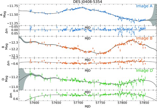
Light curves for DES J0408−5354, overlaid with our best-fitting model in black, with the grey shaded region showing the error envelope in the ROA. The colour indicates the image, with the lower panels of each image showing the microlensing behaviour relative to image A. The data points for this are calculated from equation (18), and are represented by a fourth-order polynomial in the model, shown in black.

Open in new tab Download slide

Figure 10.

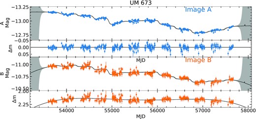
Same as Fig. 9 but for UM 673.

Open in new tab Download slide

Another interesting object was HE 0435−1223, which is a quadruply imaged quasar at z_S = 1.693, with a lens at at z_L = 0.454 (Wisotzki et al. 2002). All four images were monitored over 13 yr, providing four light curves (Millon et al. 2020a). Fig. 11 shows the results for this object. This object contained much more data than the other objects and thus it was difficulty to achieve a good fit with only a fourth-order polynomial to model the microlensing, so we used a sixth-order polynomial. We also noticed that there is a sharp increase in the brightness of image A towards its peak at an MJD ∼54250, that was unable to be fitted with a simple polynomial. Therefore we inserted an extra magnification term for image A, that of a lensing due to a point mass (Paczynski 1986). This magnification as a function of time, t, is defined as

$$\begin{eqnarray*} A\left[u(t)\right] = \frac{u^2 +2}{u \sqrt{u^2 +4}}, \quad u(t)=\sqrt{\left(\frac{t - t_0}{t_{\rm E}}\right)^2 + u_0^2}, \end{eqnarray*}$$

(19)

where we add three new parameters to the model: the time of maximum magnification, t₀, the Einstein ring radius crossing time in days, t_E, and the impact parameter, u₀, in units of the number of Einstein ring radii. We restricted the prior of t₀ to be uniform between 54 200 and 54 300 and t_E uniform between 10 and 200 d, to ensure that this fitted the sharp peak in image A. This means the model becomes

$$\begin{eqnarray*} f_{i}(t)= \left. \left\lbrace \begin{array}{@{}l@{\quad }l@{}}\left[ A_{1}X\left(t \right) + B_{1}\right] A & i=1 \\ \left[ A_{1}X\left(t -\tau _i \right) + B_{1} \right] 10^{-0.4 P_i(t)} & i\gt 1 \\ \end{array}\right. \right\rbrace \ , \end{eqnarray*}$$

(20)

where image A is the reference. If image B, C, or D is the reference, then the factor A is multiplied by |$10^{-0.4 P_i(t)}$| and the reference curve has no magnification.

Figure 11.

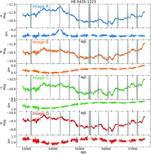
Light curves for HE 0435−122, overlaid with our best-fitting model in black, with the grey shaded region showing the error envelope in the ROA. The colour indicates the image, with the lower panels of each image showing the microlensing behaviour relative to image A. The data points for this are calculated from equation (18), and are represented by a sixth-order polynomial in the model, shown in black. For image A, magnification for lensing due to a point mass is inserted.

Open in new tab Download slide

The best-fitting values for the point mass lens are |$t_0 =54253.5^{+1.5}_{-1.5}$|⁠, |$t_{\rm E} =106.9^{+3.4}_{-3.2}$| d, and |$u_0 =1.242^{+0.017}_{-0.016}$|⁠. These values, particularly the crossing time, t_E, can be used to estimate the mass of the lens that caused this event. To do this requires the relative velocity of the object to the source and the observer, as well as the distances to the source and lens. Assuming ΛCDM cosmology with H₀ = 67.8 ± 0.9 kms⁻¹Mpc⁻¹ and Ω_m = 0.308 ± 0.012 (Planck Collaboration XIII 2016), the distance to the lens is D_L = 2600.9 Mpc for z_L = 0.454 (Wisotzki et al. 2002) and the distance to the source is D_S = 12.99 Gpc for z_S = 2.375.

From the crossing time, the Einstein ring radius can be estimated, which relates to the mass of the lens, M_L from the following :

$$\begin{eqnarray*} \frac{t_{\rm E} v_{\textrm {rel}}}{(1+z_{\rm L})D_{\rm L}} \approx \theta _{\rm E} = \sqrt{\frac{4 G M_{\rm L}}{c^2} \frac{D_{\rm S} - D_{\rm L}}{D_{\rm S} D_{\rm L}}}, \end{eqnarray*}$$

(21)

where the factor of 1 + z_L accounts for cosmic time dilation on the measured crossing time. To estimate v_rel, we would require the velocity of the source, lens, and observer, however, we can construct a prior on v_rel making some approximations, following Poindexter & Kochanek (2010) and Blackburne et al. (2014). Namely, we assume that the source velocity is negligible compared to the lens velocity due to cosmic time dilation/geometric projection effects and then construct a Gaussian prior on the relative velocity measured as the lens velocity relative to the observers velocity, estimated from the projection of the cosmic microwave background (CMB) dipole (Hinshaw et al. 2009). The width of this prior is estimated from the sum of the velocity dispersions of the source and lens galaxies to account for the random motion of stars that cause these microlensing events. For HE 0435−1223, this has been estimated to be σ_S = 227 and σ_L = 277 km s⁻¹ for the source and the lens, respectively (Blackburne et al. 2014). Therefore, the prior for the relative velocity is

$$\begin{eqnarray*} P(\pmb {v}_{\textrm {rel}}) \propto \exp \left(-\frac{\pmb {v}_{\textrm {rel}} - \pmb {v}_{\textrm {CMB}}}{2\sigma ^2}\right), \end{eqnarray*}$$

(22)

where |$\pmb {v}_{\rm {CMB}}$| is the CMB dipole velocity projected on to the lens plane, which for HE 0435−1223 is (363, −56) km s⁻¹ east and north (Blackburne et al. 2014) and the velocity dispersion is given by

$$\begin{eqnarray*} \sigma ^2 = \sigma _{\rm L}^2 + \left(\sigma _{\rm S} \frac{1+z_{\rm L}}{1+z_{\rm S}} \frac{D_{\rm L}}{D_{\rm S}}\right)^2 = (290 \ \rm {km~s {-1}})^2 . \end{eqnarray*}$$

(23)

To achieve a probability distribution of the mass of the lens, we generated a 2D probability distribution for |$\pmb {v}_{\rm {rel}}$| by sampling Gaussian random numbers with a mean of the (CMB) dipole velocity for each component and a standard deviation of 290 km s⁻¹. This is then converted into a distribution on the speed, v_rel, by taking the magnitude of each of the velocity coordinates and by also sampling Gaussian random numbers for the distribution on t_E, we calculated a probability distribution for the lens mass, M_L.

The resulting distribution is highly skewed towards low mass with a median and 16th/84th percentiles giving |$M_{\rm L} = 8^{+11}_{-6} \rm {M}_{\oplus }$|⁠. The low microlensing mass measured suggests that this object could be a planet – specifically a rogue planet that is not bound to a star. If it did orbit a star, the host star would dominate the microlensing amplification and render the planet undetectable. Such objects have been proposed to explain microlensing activity in RX J1131−1231 (Dai & Guerras 2018) where ∼ 2000 objects with masses between the Moon and Jupiter masses were estimated by analysing Fe Kα line energy shifts. Taking a larger estimate of the velocity dispersion of σ = 1000 km s⁻¹ results in a larger mass of |$M_{\rm L} = 0.16^{+0.27}_{-0.12}\, M_{\rm {Jup}}$|⁠, which is ∼ 6.7 times more massive but still a planet-mass object. The probability of a rogue planet causing this event is extremely low considering their size and suggested abundance compared with stars in the galaxy.

The other possibility is that this event is caused by a star that is moving extremely fast. Taking a typical M dwarf of ∼0.3M_⊙, would require a speed of ∼ 53 000 km s⁻¹, which is extremely fast compared to the prior – also an unlikely result. As both of these results are unlikely, it suggests that the assumption that this feature in the light curve is cause by a point-mass may be inaccurate. The caustic patterns that cause this lensing are likely much more complex than a single point mass and so while it provides a good fit to the light curve, any physical interpretation of the parameters are likely inaccurate.

The only object where we were unable to obtain a good fit was for RX J1131−1231, which similar to HE 0435−1223 is a quadruply imaged quasar (Sluse et al. 2003) that was observed for 15 yr. We had difficulty constraining the parameters for this object, specifically with the additional microlensing effect. We tried using a sixth-order polynomial as well as including point mass lenses similar to HE 0435−12234; however, we were unable to constrain these parameters. This object likely requires a more complex microlensing model. Using a higher order polynomial may work but would become overflexible at the edges of the data and so a better solution could be using a series of splines that can become more flexible where appropriate to fit certain features of the microlensing light curve. This is the approach of (Tewes et al. 2013); however, they also use splines to model the quasar variability. We have shown that the running optimal average provides a good model of the intrinsic quasar variability and so modifying our method to use splines for the microlensing variability may be a good option for these objects that have been observed for a very long period of time.

5 CONCLUSIONS

This paper presents the use of a running optimal average to model the variability of quasars, with the main aim of measuring the time delay between quasar light curves. This method can model many light curves simultaneously, providing the maximum information for determining the shape of the variability from the running optimal average. We optimize the flexibility of the ROA by calculating the effective number of parameters and minimizing the BIC through MCMC sampling of the joint posterior probability distributions of the parameters. We tested this method with mock data as well as real data in the form of gravitationally lensed quasars that were observed and analysed as part of the COSMOGRAIL project. From this testing the main findings are as follows:

Fitting to mock data with high S/N, low S/N, and large gaps, pyroa recovers precise time delays, with uncertainties comparable to javelin and significantly smaller than ICCF.
From fitting to 50 mock data sets, generated with different random walks, we verified that the uncertainties on the time delay parameters were accurate, with the normalized residuals forming a normal distribution with a mean of 0 and rms of 1.
Our method is easily able to deal with large gaps in individual light curves, either where data points from another light curve provides information within the gap of another, or the ROA interpolates across the gap with an error envelope that expands accordingly.
By including a noise model that allows the variance of flux measurements to increase, pyroa is able to recover accurate time delays when the flux errors are deliberately underestimated, while javelin fails.
By including microlensing effects, we modelled the light curves of 33 gravitationally lensed quasars from the COSMOGRAIL project. We find delays that are consistent with the previous analysis, with the exception of a few objects. We consistently finds smaller errors for the time delays between images as well as find delays for data that previously were unable to yield a measurement.

In addition to measuring the time delays between light curves, pyroa provides a model of the driving light curve that can be used for further analysis. For example, this can be used to generate a power-density spectrum of the light curves, decompose light curves into variable/fixed components to separate AGN from galaxy or inter-calibrate data from multiple telescopes where the ROA provides a model of the merged light curve. The code pyroa is publicly available, providing a new tool in reverberation mapping studies and gravitationally lensed quasars.

SUPPORTING INFORMATION

Supplementary_Material.pdf

Please note: Oxford University Press is not responsible for the content or functionality of any supporting materials supplied by the authors. Any queries (other than missing material) should be directed to the corresponding author for the article.

ACKNOWLEDGEMENTS

KH and JVHS acknowledge support from STFC grant ST/R000824/1.

DATA AVAILABILITY

The light curves for the COSMOGRAIL quasars were obtained from https://obswww.unige.ch/~millon/d3cs/COSMOGRAIL_public/. Our results for each object including a plot of the model/data, a corner plot, the MCMC samples and the individual light curves used for the fit can be found at https://dx.doi.org/10.5281/zenodo.5060008.

Footnotes

1

https://github.com/FergusDonnan/PyROA.

2

https://github.com/FergusDonnan/Running-Optimal-Average.

3

https://bitbucket.org/cgrier/python_ccf_code/src/master/.

4

https://github.com/legolason/javelin-1.

5

https://dx.doi.org/10.5281/zenodo.5060008.

REFERENCES

Blackburne

J. A.

,

Kochanek

C. S.

,

Chen

B.

,

Dai

X.

,

Chartas

G.

,

2014

,

ApJ

,

789

,

125

10.1088/0004-637X/789/2/125

Crossref

Search ADS

Blandford

R. D.

,

McKee

C. F.

,

1982

,

ApJ

,

255

,

419

10.1086/159843

Crossref

Search ADS

Bonvin

V.

et al. ,

2018

,

A&A

,

616

,

A183

10.1051/0004-6361/201833287

Crossref

Search ADS

Bonvin

V.

et al. ,

2019

,

A&A

,

629

,

A97

10.1051/0004-6361/201935921

Crossref

Search ADS

Brown

T. M.

et al. ,

2013

,

PASP

,

125

,

1031

10.1086/673168

Crossref

Search ADS

Cackett

E. M.

,

Horne

K.

,

Winkler

H.

,

2007

,

MNRAS

,

380

,

669

10.1111/j.1365-2966.2007.12098.x

Crossref

Search ADS

Cackett

E. M.

,

Bentz

M. C.

,

Kara

E.

,

2021

,

iScience

,

24

,

102557

10.1016/j.isci.2021.102557

Crossref

Search ADS

PubMed

Chan

J. H. H.

,

Millon

M.

,

Bonvin

V.

,

Courbin

F.

,

2020

,

A&A

,

636

,

A52

10.1051/0004-6361/201935423

Crossref

Search ADS

Cooke

J. H.

,

Kantowski

R.

,

1975

,

ApJ

,

195

,

L11

10.1086/181697

Crossref

Search ADS

Courbin

F.

et al. ,

2018

,

A&A

,

609

,

A71

10.1051/0004-6361/201731461

Crossref

Search ADS

Dai

X.

,

Guerras

E.

,

2018

,

ApJ

,

853

,

L27

10.3847/2041-8213/aaa5fb

Crossref

Search ADS

Dexter

J.

,

Agol

E.

,

2011

,

ApJ

,

727

,

L24

10.1088/2041-8205/727/1/L24

Crossref

Search ADS

Edelson

R.

et al. ,

2019

,

ApJ

,

870

,

123

10.3847/1538-4357/aaf3b4

Crossref

Search ADS

Eigenbrod

A.

,

Courbin

F.

,

Vuissoz

C.

,

Meylan

G.

,

Saha

P.

,

Dye

S.

,

2005

,

A&A

,

436

,

25

10.1051/0004-6361:20042422

Crossref

Search ADS

Eulaers

E.

et al. ,

2013

,

A&A

,

553

,

A121

10.1051/0004-6361/201321140

Crossref

Search ADS

Event Horizon Telescope Collaboration

,

2019

,

ApJ

,

875

,

L1

10.3847/2041-8213/ab0ec7

Crossref

Search ADS

Fabian

A. C.

,

2012

,

ARA&A

,

50

,

455

10.1146/annurev-astro-081811-125521

Crossref

Search ADS

Fausnaugh

M. M.

et al. ,

2016

,

ApJ

,

821

,

56

10.3847/0004-637X/821/1/56

Crossref

Search ADS

Foreman-Mackey

D.

,

Hogg

D. W.

,

Lang

D.

,

Goodman

J.

,

2013

,

PASP

,

125

,

306

10.1086/670067

Crossref

Search ADS

Gaskell

C. M.

,

Peterson

B. M.

,

1987

,

ApJS

,

65

,

1

10.1086/191216

Crossref

Search ADS

Gehrels

N.

et al. ,

2004

,

ApJ

,

611

,

1005

10.1086/422091

Crossref

Search ADS

Gravity Collaboration

,

2018

,

Nature

,

563

,

657

10.1038/s41586-018-0731-9

Crossref

Search ADS

PubMed

Grier

C. J.

et al. ,

2017

,

ApJ

,

851

,

21

10.3847/1538-4357/aa98dc

Crossref

Search ADS

Heckman

T. M.

,

Best

P. N.

,

2014

,

ARA&A

,

52

,

589

10.1146/annurev-astro-081913-035722

Crossref

Search ADS

Hernández Santisteban

J. V.

et al. ,

2020

,

MNRAS

,

498

,

5399

10.1093/mnras/staa2365

Crossref

Search ADS

Hinshaw

G.

et al. ,

2009

,

ApJS

,

180

,

225

10.1088/0067-0049/180/2/225

Crossref

Search ADS

Homayouni

Y.

et al. ,

2021

,

preprint (arXiv:2105.02884)

Horne

K.

,

Peterson

B. M.

,

Collier

S. J.

,

Netzer

H.

,

2004

,

PASP

,

116

,

465

10.1086/420755

Crossref

Search ADS

Kara

E.

et al. ,

2021

,

preprint (arXiv:2105.05840)

Karson

M.

,

1968

,

J. Am. Stat. Assoc.

,

63

,

1047

10.1080/01621459.1968.11009335

Crossref

Search ADS

Kawaguchi

T.

,

Mineshige

S.

,

Umemura

M.

,

Turner

E. L.

,

1998

,

ApJ

,

504

,

671

10.1086/306105

Crossref

Search ADS

Koptelova

E.

et al. ,

2012

,

A&A

,

544

,

A51

10.1051/0004-6361/201116645

Crossref

Search ADS

Kozłowski

S.

et al. ,

2010

,

ApJ

,

708

,

927

10.1088/0004-637X/708/2/927

Crossref

Search ADS

Lin

H.

et al. ,

2017

,

ApJ

,

838

,

L15

10.3847/2041-8213/aa624e

Crossref

Search ADS

Lynden-Bell

D.

,

1969

,

Nature

,

223

,

690

10.1038/223690a0

Crossref

Search ADS

MacLeod

C. L.

et al. ,

2010

,

ApJ

,

721

,

1014

10.1088/0004-637X/721/2/1014

Crossref

Search ADS

Millon

M.

et al. ,

2020a

,

A&A

,

640

,

A105

10.1051/0004-6361/202037740

Crossref

Search ADS

Millon

M.

et al. ,

2020b

,

A&A

,

642

,

A193

10.1051/0004-6361/202038698

Crossref

Search ADS

Oscoz

A.

,

Serra-Ricart

M.

,

Mediavilla

E.

,

Muñoz

J. A.

,

2013

,

ApJ

,

779

,

144

10.1088/0004-637X/779/2/144

Crossref

Search ADS

Paczynski

B.

,

1986

,

ApJ

,

304

,

1

10.1086/164140

Crossref

Search ADS

Peterson

B. M.

,

1993

,

PASP

,

105

,

247

10.1086/133140

Crossref

Search ADS

Peterson

B. M.

,

Wanders

I.

,

Horne

K.

,

Collier

S.

,

Alexander

T.

,

Kaspi

S.

,

Maoz

D.

,

1998

,

PASP

,

110

,

660

10.1086/316177

Crossref

Search ADS

Peterson

B. M.

et al. ,

2004

,

ApJ

,

613

,

682

10.1086/423269

Crossref

Search ADS

Planck Collaboration

et al. .,

2016

,

A&A

,

594

,

A13

10.1051/0004-6361/201525830

Crossref

Search ADS

Poindexter

S.

,

Kochanek

C. S.

,

2010

,

ApJ

,

712

,

658

10.1088/0004-637X/712/1/658

Crossref

Search ADS

Rathna Kumar

S.

et al. ,

2013

,

A&A

,

557

,

A44

10.1051/0004-6361/201322116

Crossref

Search ADS

Refsdal

S.

,

1964

,

MNRAS

,

128

,

295

10.1093/mnras/128.4.295

Crossref

Search ADS

Salpeter

E. E.

,

1964

,

ApJ

,

140

,

796

10.1086/147973

Crossref

Search ADS

Sanders

D. B.

,

Phinney

E. S.

,

Neugebauer

G.

,

Soifer

B. T.

,

Matthews

K.

,

1989

,

ApJ

,

347

,

29

10.1086/168094

Crossref

Search ADS

Shapiro

I. I.

,

1964

,

Phys. Rev. Lett.

,

13

,

789

10.1103/PhysRevLett.13.789

Crossref

Search ADS

Shen

Y.

et al. ,

2015

,

ApJS

,

216

,

4

10.1088/0067-0049/216/1/4

Crossref

Search ADS

Sluse

D.

,

Tewes

M.

,

2014

,

A&A

,

571

,

A60

10.1051/0004-6361/201424776

Crossref

Search ADS

Sluse

D.

et al. ,

2003

,

A&A

,

406

,

L43

10.1051/0004-6361:20030904

Crossref

Search ADS

Starkey

D. A.

,

Horne

K.

,

Villforth

C.

,

2016

,

MNRAS

,

456

,

1960

10.1093/mnras/stv2744

Crossref

Search ADS

Sun

M.

,

Grier

C. J.

,

Peterson

B. M.

,

2018

,

Astrophysics Source Code Library

,

record ascl:1805.032

Tewes

M.

et al. ,

2012

,

The Messenger

,

150

,

49

Tewes

M.

,

Courbin

F.

,

Meylan

G.

,

2013

,

A&A

,

553

,

A120

10.1051/0004-6361/201220123

Crossref

Search ADS

Williams

P. R.

et al. ,

2021

,

ApJ

,

911

,

64

10.3847/1538-4357/abe943

Crossref

Search ADS

Wisotzki

L.

,

Schechter

P. L.

,

Bradt

H. V.

,

Heinmüller

J.

,

Reimers

D.

,

2002

,

A&A

,

395

,

17

10.1051/0004-6361:20021213

Crossref

Search ADS

Yu

Z.

,

Kochanek

C. S.

,

Peterson

B. M.

,

Zu

Y.

,

Brandt

W. N.

,

Cackett

E. M.

,

Fausnaugh

M. M.

,

McHardy

I. M.

,

2020

,

MNRAS

,

491

,

6045

10.1093/mnras/stz3464

Crossref

Search ADS

Zu

Y.

,

Kochanek

C. S.

,

Peterson

B. M.

,

2011

,

ApJ

,

735

,

80

10.1088/0004-637X/735/2/80

Crossref

Search ADS

This article is published and distributed under the terms of the Oxford University Press, Standard Journals Publication Model (https://dbpia.nl.go.kr/journals/pages/open_access/funder_policies/chorus/standard_publication_model)

Download all slides

Object	Images	Time delays (d)		Microlensing coeff. (mag)							Ref.
		This work	COSMOGRAIL	P_{i, 0}	P_{i, 1}	P_{i, 2}	P_{i, 3}	P_{i, 4}	P_{i, 5}	P_{i, 6}
2M 1134−2103	AB	\|$-29.53^{+0.63}_{-0.59}$\|	−30.5 ± 2.2	\|$0.038\,35^{+0.000\,47}_{-0.000\,44}$\|	\|$-0.0027^{+0.0013}_{-0.0012}$\|	\|$-0.0107^{+0.0035}_{-0.0035}$\|	\|$0.0259^{+0.0030}_{-0.0030}$\|	\|$-0.0009^{+0.0046}_{-0.0049}$\|	–	–	Millon et al. (2020b)
	AC	\|$8.78^{+0.56}_{-0.56}$\|	8.6 ± 1.4	\|$0.065\,02^{+0.000\,39}_{-0.000\,39}$\|	\|$0.0021^{+0.0011}_{-0.0011}$\|	\|$-0.0015^{+0.0027}_{-0.0027}$\|	\|$0.0003^{+0.0018}_{-0.0017}$\|	\|$0.0033^{+0.0031}_{-0.0032}$\|	–	–
	AD	\|$-65.6^{+2.6}_{-2.3}$\|	−71.9 ± 6.7	\|$1.7559^{+0.0011}_{-0.0011}$\|	\|$-0.0110^{+0.0064}_{-0.0058}$\|	\|$0.0151^{+0.0083}_{-0.0084}$\|	\|$0.038^{+0.015}_{-0.016}$\|	\|$-0.028^{+0.015}_{-0.014}$\|	–	–
	BC	\|$38.60^{+0.49}_{-0.50}$\|	38.9 ± 2.2	\|$0.027\,91^{+0.000\,43}_{-0.000\,42}$\|	\|$0.0005^{+0.0019}_{-0.0019}$\|	\|$-0.0202^{+0.0030}_{-0.0030}$\|	\|$-0.0156^{+0.0056}_{-0.0056}$\|	\|$0.0137^{+0.0056}_{-0.0058}$\|	–	–
	BD	\|$-36.4^{+1.9}_{-2.0}$\|	−41.5 ± 7.6	\|$1.7186^{+0.0011}_{-0.0011}$\|	\|$-0.0288^{+0.0065}_{-0.0066}$\|	\|$0.0592^{+0.0077}_{-0.0078}$\|	\|$0.028^{+0.014}_{-0.013}$\|	\|$-0.048^{+0.013}_{-0.013}$\|	–	–
	CD	\|$-75.6^{+2.4}_{-2.2}$\|	−80.5 ± 6.8	\|$1.6927^{+0.0011}_{-0.0011}$\|	\|$-0.0153^{+0.0057}_{-0.0056}$\|	\|$0.0092^{+0.0096}_{-0.0096}$\|	\|$0.059^{+0.016}_{-0.018}$\|	\|$-0.040^{+0.015}_{-0.015}$\|	–	–
DES J0407−5006	AB	\|$-123.9^{+1.5}_{-1.5}$\|	−128.4 ± 3.6	\|$1.2479^{+0.0016}_{-0.0016}$\|	\|$-0.070^{+0.014}_{-0.013}$\|	\|$0.126^{+0.023}_{-0.024}$\|	\|$-0.010^{+0.012}_{-0.012}$\|	\|$-0.051^{+0.016}_{-0.016}$\|	–	–	Millon et al. (2020b)
DES J0408−5354	AB	\|$-113.77^{+0.79}_{-0.76}$\|	−112.1 ± 2.1	\|$-0.6047^{+0.0054}_{-0.0059}$\|	\|$-0.012^{+0.036}_{-0.036}$\|	\|$-0.072^{+0.054}_{-0.052}$\|	\|$0.008^{+0.042}_{-0.041}$\|	\|$0.042^{+0.041}_{-0.048}$\|	–	–	Courbin et al. (2018)
	AD	\|$-159.1^{+1.8}_{-1.7}$\|	−155.5 ± 12.8	\|$0.511^{+0.020}_{-0.021}$\|	\|$-0.017^{+0.065}_{-0.066}$\|	\|$-0.134^{+0.072}_{-0.068}$\|	\|$-0.017^{+0.094}_{-0.010}$\|	\|$0.186^{+0.074}_{-0.067}$\|	–	–
	BD	\|$-47.6^{+1.3}_{-1.4}$\|	−42.4 ± 17.6	\|$1.1244^{+0.0043}_{-0.0039}$\|	\|$-0.0643^{+0.0092}_{-0.0087}$\|	\|$-0.096^{+0.027}_{-0.029}$\|	\|$0.111^{+0.023}_{-0.022}$\|	\|$0.077^{+0.031}_{-0.031}$\|	–	–
DES 2325−5229	AB	\|$44.83^{+0.90}_{-0.87}$\|	43.9 ± 4.2	\|$1.0985^{+0.0040}_{-0.0041}$\|	\|$-0.131^{+0.011}_{-0.011}$\|	\|$0.045^{+0.037}_{-0.037}$\|	\|$0.397^{+0.033}_{-0.032}$\|	\|$0.037^{+0.050}_{-0.049}$\|	–	–	Millon et al. (2020b)
HE 0047−1756	AB	\|$-11.00^{+0.39}_{-0.39}$\|	−10.8 ± 1.0	\|$1.6127^{+0.0014}_{-0.0013}$\|	\|$-0.0140^{+0.0029}_{-0.0029}$\|	\|$0.0617^{+0.0060}_{-0.0064}$\|	\|$0.0235^{+0.0040}_{-0.0040}$\|	\|$-0.0550^{+0.0066}_{-0.0063}$\|	–	–	Millon et al. (2020b)
HE 0230−2130	AC	\|$17.7^{+2.1}_{-2.1}$\|	15.7 ± 3.9	\|$1.5081^{+0.0070}_{-0.0068}$\|	\|$-0.129^{+0.013}_{-0.013}$\|	\|$0.202^{+0.047}_{-0.047}$\|	\|$-0.002^{+0.017}_{-0.018}$\|	\|$-0.139^{+0.049}_{-0.051}$\|	–	–	Millon et al. (2020a)
	AD	\|$-10.5^{+9.8}_{-6.1}$\|	–	\|$2.321^{+0.014}_{-0.016}$\|	\|$-0.107^{+0.024}_{-0.024}$\|	\|$0.183^{+0.089}_{-0.086}$\|	\|$-0.098^{+0.032}_{-0.031}$\|	\|$-0.226^{+0.089}_{-0.092}$\|	–	–
	CD	\|$-26.9^{+11.4}_{-7.1}$\|	–	\|$0.802^{+0.014}_{-0.015}$\|	\|$0.035^{+0.029}_{-0.029}$\|	\|$0.004^{+0.010}_{-0.093}$\|	\|$-0.111^{+0.039}_{-0.039}$\|	\|$-0.11^{+0.10}_{-0.10}$\|	–	–
HE 0435−1223	AB	\|$-8.00^{+0.37}_{-0.36}$\|	−9.0 ± 0.8	\|$0.2555^{+0.0019}_{-0.0019}$\|	\|$-0.4259^{+0.0073}_{-0.0068}$\|	\|$0.887^{+0.021}_{-0.021}$\|	\|$0.793^{+0.024}_{-0.025}$\|	\|$-1.910^{+0.056}_{-0.055}$\|	\|$0.546^{+0.020}_{-0.020}$\|	\|$0.932^{+0.038}_{-0.039}$\|	Millon et al. (2020a)
	AC	\|$-0.12^{+0.26}_{-0.20}$\|	−0.8 ± 0.7	\|$0.6614^{+0.0017}_{-0.0017}$\|	\|$-0.4137^{+0.0068}_{-0.0068}$\|	\|$0.773^{+0.020}_{-0.019}$\|	\|$0.497^{+0.023}_{-0.023}$\|	\|$-1.438^{+0.049}_{-0.052}$\|	\|$-0.218^{+0.018}_{-0.019}$\|	\|$0.674^{+0.036}_{-0.033}$\|
	AD	\|$-13.99^{+0.19}_{-0.27}$\|	−13.8 ± 0.8	\|$1.2895^{+0.0019}_{-0.0020}$\|	\|$-0.1620^{+0.0074}_{-0.0074}$\|	\|$0.781^{+0.022}_{-0.022}$\|	\|$0.369^{+0.026}_{-0.025}$\|	\|$-1.678^{+0.059}_{-0.060}$\|	\|$-0.202^{+0.020}_{-0.021}$\|	\|$0.902^{+0.041}_{-0.041}$\|
	BC	\|$9.06^{+0.20}_{-0.28}$\|	7.8 ± 0.9	\|$0.4069^{+0.0018}_{-0.0018}$\|	\|$0.0076^{+0.0051}_{-0.0054}$\|	\|$-0.121^{+0.019}_{-0.019}$\|	\|$-0.275^{+0.019}_{-0.018}$\|	\|$0.480^{+0.049}_{-0.049}$\|	\|$0.314^{+0.016}_{-0.016}$\|	\|$-0.257^{+0.033}_{-0.034}$\|
	BD	\|$-5.22^{+0.39}_{-0.41}$\|	−5.4 ± 0.8	\|$1.0326^{+0.0020}_{-0.0020}$\|	\|$0.2693^{+0.0059}_{-0.0061}$\|	\|$-0.101^{+0.022}_{-0.023}$\|	\|$-0.448^{+0.021}_{-0.021}$\|	\|$0.228^{+0.058}_{-0.056}$\|	\|$0.363^{+0.018}_{-0.018}$\|	\|$-0.032^{+0.039}_{-0.040}$\|
	CD	\|$-13.99^{+0.19}_{-0.30}$\|	−13.2 ± 0.8	\|$0.6254^{+0.0019}_{-0.0019}$\|	\|$0.2609^{+0.0057}_{-0.0057}$\|	\|$0.017^{+0.020}_{-0.020}$\|	\|$-0.163^{+0.020}_{-0.021}$\|	\|$-0.247^{+0.050}_{-0.051}$\|	\|$0.041^{+0.018}_{-0.017}$\|	\|$0.229^{+0.036}_{-0.035}$\|
HE 2149−2745	AB	\|$-71.3^{+3.3}_{-3.4}$\|	−39.0 ± 15.8	\|$1.4350^{+0.0018}_{-0.0018}$\|	\|$-0.0390^{+0.0050}_{-0.0050}$\|	\|$-0.184^{+0.014}_{-0.013}$\|	\|$-0.1197^{+0.0078}_{-0.0081}$\|	\|$0.175^{+0.015}_{-0.016}$\|	–	–	Millon et al. (2020a)
HS 0818+1227	AB	\|$-39.8^{+3.3}_{-3.2}$\|	−153.8 ± 13.9	\|$1.9478^{+0.0040}_{-0.0041}$\|	\|$0.1287^{+0.0081}_{-0.0080}$\|	\|$0.102^{+0.023}_{-0.023}$\|	\|$-0.038^{+0.011}_{-0.011}$\|	\|$-0.116^{+0.023}_{-0.024}$\|	–	–	Millon et al. (2020a)
HS 2209+1914	AB	\|$24.0^{+2.4}_{-2.4}$\|	20.0 ± 5.0	\|$0.216\,99^{+0.0000\,53}_{-0.000\,55}$\|	\|$0.0196^{+0.0030}_{-0.0029}$\|	\|$-0.0071^{+0.0064}_{-0.0066}$\|	\|$0.0870^{+0.0059}_{-0.0059}$\|	\|$0.0707^{+0.0092}_{-0.0091}$\|	–	–	Eulaers et al. (2013)
Q J0158−4325	AB	\|$-34.9^{+3.2}_{-3.0}$\|	−22.7 ± 3.6	\|$1.1236^{+0.0031}_{-0.0031}$\|	\|$0.6289^{+0.0071}_{-0.0072}$\|	\|$-0.148^{+0.020}_{-0.020}$\|	\|$-0.075^{+0.011}_{-0.010}$\|	\|$-0.027^{+0.022}_{-0.022}$\|	–	–	Millon et al. (2020a)
SDSS J0246−0825	AB	\|$3.1^{+2.0}_{-2.0}$\|	0.8 ± 5.1	\|$1.8400^{+0.0051}_{-0.0050}$\|	\|$0.476^{+0.013}_{-0.013}$\|	\|$-0.892^{+0.035}_{-0.034}$\|	\|$-0.314^{+0.020}_{-0.020}$\|	\|$0.673^{+0.037}_{-0.038}$\|	–	–	Millon et al. (2020a)
SDSS J0832+0404	AB	\|$-136.5^{+1.8}_{-1.9}$\|	−125.3 ± 18.1	\|$0.9912^{+0.0064}_{-0.0066}$\|	\|$-0.066^{+0.018}_{-0.019}$\|	\|$-0.009^{+0.042}_{-0.043}$\|	\|$-0.416^{+0.026}_{-0.024}$\|	\|$0.346^{+0.048}_{-0.047}$\|	–	–	Millon et al. (2020a)
SDSS J0924+0219	AB	\|$0.6^{+2.7}_{-2.6}$\|	2.4 ± 3.8	\|$1.3827^{+0.0055}_{-0.0056}$\|	\|$-0.014^{+0.015}_{-0.015}$\|	\|$0.291^{+0.038}_{-0.039}$\|	\|$0.476^{+0.023}_{-0.024}$\|	\|$-0.693^{+0.046}_{-0.047}$\|	–	–	Millon et al. (2020a)
	AC	\|$-30.9^{+7.9}_{-8.0}$\|	–	\|$2.785^{+0.017}_{-0.017}$\|	\|$0.082^{+0.047}_{-0.045}$\|	\|$0.14^{+0.11}_{-0.11}$\|	\|$0.827^{+0.081}_{-0.077}$\|	\|$-0.54^{+0.14}_{-0.13}$\|	–	–
	BC	\|$-32.5^{+8.4}_{-8.5}$\|	–	\|$1.401^{+0.018}_{-0.018}$\|	\|$0.099^{+0.049}_{-0.046}$\|	\|$-0.13^{+0.12}_{-0.12}$\|	\|$0.325^{+0.081}_{-0.083}$\|	\|$0.16^{+0.15}_{-0.14}$\|	–	–
SDSS J1001+5027	AB	\|$-119.9^{+1.4}_{-1.5}$\|	−119.3 ± 3.3	\|$0.420\,39^{+0.000\,10}_{-0.000\,93}$\|	\|$0.0004^{+0.0039}_{-0.000\,41}$\|	\|$0.0069^{+0.0089}_{-0.000\,91}$\|	\|$-0.0215^{+0.0081}_{-0.0080}$\|	\|$-0.024^{+0.014}_{-0.013}$\|	–	–	Rathna Kumar et al. (2013)
SDSS J1206+4332	AB	\|$-113.0^{+1.1}_{-1.2}$\|	−111.3 ± 3.0	\|$0.3332^{+0.0023}_{-0.0022}$\|	\|$-0.1670^{+0.0075}_{-0.0073}$\|	\|$-0.213^{+0.016}_{-0.016}$\|	\|$0.104^{+0.015}_{-0.015}$\|	\|$0.141^{+0.023}_{-0.023}$\|	–	–	Eulaers et al. (2013)
SDSS J1226−0006	AB	\|$25.63^{+0.89}_{-0.76}$\|	–	\|$0.9113^{+0.0025}_{-0.0024}$\|	\|$0.2639^{+0.0055}_{-0.0056}$\|	\|$0.160^{+0.016}_{-0.016}$\|	\|$-0.1019^{+0.0079}_{-0.0080}$\|	\|$-0.082^{+0.017}_{-0.017}$\|	–	–	Millon et al. (2020a)
SDSS J1320+1644	AB	\|$-157.1^{+14.2}_{-14.9}$\|	–	\|$0.894^{+0.031}_{-0.028}$\|	\|$0.178^{+0.053}_{-0.066}$\|	\|$-0.24^{+0.24}_{-0.39}$\|	\|$-0.025^{+0.066}_{-0.070}$\|	\|$0.04^{+0.28}_{-0.19}$\|	–	–	Millon et al. (2020a)
SDSS J1322+1052	AB	\|$105.6^{+10.0}_{-11.5}$\|	–	\|$1.6613^{+0.0068}_{-0.0070}$\|	\|$-0.077^{+0.023}_{-0.024}$\|	\|$-0.474^{+0.053}_{-0.053}$\|	\|$0.223^{+0.040}_{-0.039}$\|	\|$0.581^{+0.063}_{-0.065}$\|	–	–	Millon et al. (2020a)
SDSS J1335+0118	AB	\|$-59.0^{+4.1}_{-4.2}$\|	−56.0 ± 5.9	\|$1.0958^{+0.0020}_{-0.0021}$\|	\|$-0.1001^{+0.0046}_{-0.0046}$\|	\|$-0.038^{+0.013}_{-0.013}$\|	\|$0.0144^{+0.0065}_{-0.0072}$\|	\|$0.051^{+0.014}_{-0.014}$\|	–	–	Millon et al. (2020a)
SDSS J1349+1227	AB	\|$-140.8^{+7.5}_{-6.5}$\|	–	\|$1.3180^{+0.0056}_{-0.0069}$\|	\|$-0.007^{+0.013}_{-0.012}$\|	\|$0.020^{+0.039}_{-0.036}$\|	\|$0.089^{+0.018}_{-0.018}$\|	\|$0.005^{+0.039}_{-0.041}$\|	–	–	Millon et al. (2020a)
SDSS J1405+0959	AB	\|$-82.8^{+12.3}_{-19.7}$\|	–	\|$0.778^{+0.011}_{-0.010}$\|	\|$0.019^{+0.024}_{-0.024}$\|	\|$0.023^{+0.060}_{-0.061}$\|	\|$-0.004^{+0.033}_{-0.034}$\|	\|$0.035^{+0.069}_{-0.069}$\|	–	–	Millon et al. (2020a)
SDSS J1455+1447	AB	\|$-43.4^{+2.3}_{-2.2}$\|	−47.2 ± 7.6	\|$1.0711^{+0.0041}_{-0.0039}$\|	\|$0.0426^{+0.0084}_{-0.0088}$\|	\|$0.002^{+0.026}_{-0.026}$\|	\|$0.007^{+0.012}_{-0.012}$\|	\|$0.024^{+0.027}_{-0.028}$\|	–	–	Millon et al. (2020a)
SDSS J1515+1511	AB	\|$-208.3^{+1.8}_{-1.8}$\|	−210.2 ± 5.6	\|$0.3679^{+0.0022}_{-0.0024}$\|	\|$0.0117^{+0.0070}_{-0.0067}$\|	\|$-0.027^{+0.021}_{-0.019}$\|	\|$-0.025^{+0.019}_{-0.019}$\|	\|$0.053^{+0.032}_{-0.035}$\|	–	–	Millon et al. (2020a)
SDSS J1620+1203	AB	\|$-158.3^{+2.4}_{-2.5}$\|	−171.5 ± 8.7	\|$1.2387^{+0.0064}_{-0.0067}$\|	\|$0.003^{+0.016}_{-0.016}$\|	\|$-0.082^{+0.048}_{-0.045}$\|	\|$-0.093^{+0.037}_{-0.036}$\|	\|$0.148^{+0.061}_{-0.062}$\|	–	–	Millon et al. (2020a)
PG 1115+080	AB	\|$-6.90^{+0.68}_{-0.69}$\|	−8.3 ± 1.5	\|$2.5709^{+0.0018}_{-0.0018}$\|	\|$0.0211^{+0.0041}_{-0.0041}$\|	\|$0.037^{+0.012}_{-0.012}$\|	\|$-0.0103^{+0.0060}_{-0.0059}$\|	\|$-0.034^{+0.013}_{-0.012}$\|	–	–	Bonvin et al. (2018)
	AC	\|$9.43^{+0.83}_{-0.82}$\|	9.9 ± 1.1	\|$2.2193^{+0.0017}_{-0.0016}$\|	\|$0.0040^{+0.0035}_{-0.0035}$\|	\|$0.033^{+0.010}_{-0.010}$\|	\|$-0.0048^{+0.0066}_{-0.0063}$\|	\|$-0.038^{+0.012}_{-0.012}$\|	–	–
	BC	\|$-16.35^{+0.94}_{-0.90}$\|	18.8 ± 1.6	\|$-0.3569^{+0.0022}_{-0.0023}$\|	\|$-0.0268^{+0.0053}_{-0.0051}$\|	\|$0.012^{+0.012}_{-0.011}$\|	\|$0.0255^{+0.0098}_{-0.0099}$\|	\|$-0.009^{+0.014}_{-0.014}$\|	–	–
PSJ 1606−2333	AB	\|$-12.9^{+1.1}_{-1.1}$\|	−10.4 ± 2.2	\|$0.1523^{+0.0029}_{-0.0030}$\|	\|$0.0342^{+0.0046}_{-0.0048}$\|	\|$0.001^{+0.012}_{-0.011}$\|	\|$-0.0186^{+0.0074}_{-0.0074}$\|	\|$-0.011^{+0.012}_{-0.013}$\|	–	–	Millon et al. (2020b)
	AC	\|$-30.6^{+2.2}_{-2.4}$\|	−29.2 ± 4.7	\|$0.5593^{+0.0059}_{-0.0060}$\|	\|$0.0338^{+0.0050}_{-0.0053}$\|	\|$-0.056^{+0.022}_{-0.023}$\|	\|$0.001^{+0.010}_{-0.010}$\|	\|$0.003^{+0.023}_{-0.023}$\|	–	–
	AD	\|$-40.1^{+2.8}_{-2.4}$\|	−45.7 ± 10.9	\|$0.7449^{+0.0071}_{-0.0069}$\|	\|$0.0689^{+0.0066}_{-0.0064}$\|	\|$-0.037^{+0.025}_{-0.025}$\|	\|$-0.004^{+0.014}_{-0.014}$\|	\|$-0.022^{+0.024}_{-0.024}$\|	–	–
	BC	\|$-17.5^{+1.8}_{-2.0}$\|	−19.3 ± 4.5	\|$0.4114^{+0.0045}_{-0.0049}$\|	\|$-0.0011^{+0.0054}_{-0.0054}$\|	\|$-0.056^{+0.021}_{-0.020}$\|	\|$0.0161^{+0.0090}_{-0.0091}$\|	\|$0.005^{+0.020}_{-0.021}$\|	–	–
	BD	\|$-27.4^{+3.2}_{-2.7}$\|	−36.2 ± 10.4	\|$0.5986^{+0.0064}_{-0.0061}$\|	\|$0.0349^{+0.0064}_{-0.0066}$\|	\|$-0.038^{+0.024}_{-0.027}$\|	\|$0.0119^{+0.013}_{-0.012}$\|	\|$-0.023^{+0.025}_{-0.024}$\|	–	–
	CD	\|$-9.0^{+3.9}_{-3.4}$\|	−13.8 ± 8.4	\|$0.1874^{+0.0084}_{-0.0073}$\|	\|$0.0262^{+0.0066}_{-0.0075}$\|	\|$0.034^{+0.028}_{-0.032}$\|	\|$0.002^{+0.011}_{-0.010}$\|	\|$-0.047^{+0.026}_{-0.025}$\|	–	–
Q 1355−2257	AB	\|$-64.5^{+4.6}_{-4.7}$\|	−81.5 ± 11.4	\|$1.5528^{+0.0049}_{-0.0049}$\|	\|$-0.120^{+0.015}_{-0.015}$\|	\|$0.287^{+0.039}_{-0.039}$\|	\|$0.005^{+0.037}_{-0.037}$\|	\|$-0.259^{+0.059}_{-0.058}$\|	–	–	Millon et al. (2020a)
Q 2237+0305	AB	\|$11.7^{+4.7}_{-5.4}$\|	–	\|$0.8885^{+0.0050}_{-0.0051}$\|	\|$-0.128^{+0.016}_{-0.016}$\|	\|$0.139^{+0.034}_{-0.034}$\|	\|$0.021^{+0.023}_{-0.022}$\|	\|$-0.127^{+0.037}_{-0.035}$\|	–	–	Millon et al. (2020a)
UM 673	AB	\|$7.7^{+10.6}_{-13.0}$\|	−97.7 ± 15.8	\|$2.1667^{+0.0022}_{-0.0022}$\|	\|$0.0170^{+0.0066}_{-0.0066}$\|	\|$-0.127^{+0.015}_{-0.015}$\|	\|$-0.008^{+0.010}_{-0.010}$\|	\|$0.176^{+0.016}_{-0.016}$\|	–	–	Millon et al. (2020a)
WFI J2026−4536	AB	\|$4.4^{+2.1}_{-2.3}$\|	18.0 ± 4.8	\|$1.9398^{+0.0027}_{-0.0029}$\|	\|$-0.1713^{+0.0075}_{-0.0075}$\|	\|$0.255^{+0.018}_{-0.019}$\|	\|$0.108^{+0.011}_{-0.012}$\|	\|$-0.224^{+0.021}_{-0.021}$\|	–	–	Millon et al. (2020a)
	AC	\|$2.6^{+4.2}_{-4.6}$\|	–	\|$2.0434^{+0.0050}_{-0.0050}$\|	\|$-0.031^{+0.014}_{-0.014}$\|	\|$0.246^{+0.035}_{-0.036}$\|	\|$-0.023^{+0.022}_{-0.022}$\|	\|$-0.196^{+0.041}_{-0.041}$\|	–	–
	BC	\|$2.2^{+5.1}_{-5.5}$\|	–	\|$0.1031^{+0.0056}_{-0.0055}$\|	\|$0.144^{+0.015}_{-0.016}$\|	\|$-0.006^{+0.039}_{-0.039}$\|	\|$0.137^{+0.025}_{-0.024}$\|	\|$0.025^{+0.046}_{-0.045}$\|	–	–
WFI 2033−4723	AB	\|$40.54^{+0.60}_{-0.64}$\|	36.2 ± 0.7	\|$1.0681^{+0.0013}_{-0.0012}$\|	\|$-0.0072^{+0.0030}_{-0.0030}$\|	\|$0.0349^{+0.0083}_{-0.0081}$\|	\|$0.0390^{+0.0052}_{-0.0050}$\|	\|$0.019^{+0.010}_{-0.010}$\|	–	–	Bonvin et al. (2019)
	AC	\|$-27.23^{+0.69}_{-0.66}$\|	−23.3 ± 1.3	\|$1.3830^{+0.0014}_{-0.0014}$\|	\|$0.0766^{+0.0033}_{-0.0033}$\|	\|$-0.0752^{+0.0086}_{-0.0091}$\|	\|$-0.0077^{+0.0054}_{-0.0055}$\|	\|$0.000^{+0.010}_{-0.011}$\|	–	–
	BC	\|$-68.3^{+1.2}_{-0.8}$\|	−59.4 ± 1.3	\|$0.3146^{+0.0016}_{-0.0016}$\|	\|$0.0859^{+0.0041}_{-0.0040}$\|	\|$-0.106^{+0.011}_{-0.012}$\|	\|$-0.0456^{+0.0066}_{-0.0069}$\|	\|$-0.021^{+0.014}_{-0.014}$\|	–	–
WG 0214−2105	AB	\|$10.24^{+0.67}_{-0.64}$\|	7.5 ± 2.8	\|$-0.0773^{+0.0043}_{-0.0042}$\|	\|$-0.1127^{+0.0052}_{-0.0054}$\|	\|$0.031^{+0.019}_{-0.019}$\|	\|$0.0632^{+0.0080}_{-0.0076}$\|	\|$-0.0635^{+0.0018}_{-0.0018}$\|	–	–	Millon et al. (2020b)
	AC	\|$-5.82^{+0.69}_{-0.69}$\|	−6.7 ± 3.6	\|$-0.0413^{+0.0041}_{-0.0041}$\|	\|$-0.0320^{+0.0057}_{-0.0057}$\|	\|$-0.020^{+0.019}_{-0.019}$\|	\|$0.0118^{+0.0083}_{-0.0086}$\|	\|$0.012^{+0.018}_{-0.018}$\|	–	–
	AD	\|$-43.2^{+1.8}_{-1.8}$\|	−14.1 ± 4.9	\|$0.6228^{+0.0079}_{-0.0078}$\|	\|$-0.111^{+0.013}_{-0.013}$\|	\|$0.403^{+0.036}_{-0.035}$\|	\|$0.241^{+0.023}_{-0.023}$\|	\|$-0.339^{+0.038}_{-0.039}$\|	–	–
	BC	\|$-16.01^{+0.56}_{-0.59}$\|	−14.2 ± 2.6	\|$0.0314^{+0.0043}_{-0.0043}$\|	\|$0.0840^{+0.0058}_{-0.0058}$\|	\|$-0.047^{+0.019}_{-0.019}$\|	\|$-0.0657^{+0.0093}_{-0.0090}$\|	\|$0.083^{+0.020}_{-0.019}$\|	–	–
	BD	\|$-53.5^{+1.7}_{-1.7}$\|	−21.6 ± 4.6	\|$0.6812^{+0.0079}_{-0.0078}$\|	\|$0.007^{+0.014}_{-0.014}$\|	\|$0.413^{+0.036}_{-0.037}$\|	\|$0.131^{+0.024}_{-0.024}$\|	\|$-0.271^{+0.040}_{-0.041}$\|	–	–
	CD	\|$-37.4^{+1.6}_{-1.6}$\|	−7.5 ± 4.7	\|$0.6616^{+0.0074}_{-0.0077}$\|	\|$-0.083^{+0.012}_{-0.012}$\|	\|$0.422^{+0.035}_{-0.035}$\|	\|$0.232^{+0.020}_{-0.020}$\|	\|$-0.346^{+0.037}_{-0.038}$\|	–	–

Object	Images	Time delays (d)		Microlensing coeff. (mag)							Ref.
		This work	COSMOGRAIL	P_{i, 0}	P_{i, 1}	P_{i, 2}	P_{i, 3}	P_{i, 4}	P_{i, 5}	P_{i, 6}
2M 1134−2103	AB	\|$-29.53^{+0.63}_{-0.59}$\|	−30.5 ± 2.2	\|$0.038\,35^{+0.000\,47}_{-0.000\,44}$\|	\|$-0.0027^{+0.0013}_{-0.0012}$\|	\|$-0.0107^{+0.0035}_{-0.0035}$\|	\|$0.0259^{+0.0030}_{-0.0030}$\|	\|$-0.0009^{+0.0046}_{-0.0049}$\|	–	–	Millon et al. (2020b)
	AC	\|$8.78^{+0.56}_{-0.56}$\|	8.6 ± 1.4	\|$0.065\,02^{+0.000\,39}_{-0.000\,39}$\|	\|$0.0021^{+0.0011}_{-0.0011}$\|	\|$-0.0015^{+0.0027}_{-0.0027}$\|	\|$0.0003^{+0.0018}_{-0.0017}$\|	\|$0.0033^{+0.0031}_{-0.0032}$\|	–	–
	AD	\|$-65.6^{+2.6}_{-2.3}$\|	−71.9 ± 6.7	\|$1.7559^{+0.0011}_{-0.0011}$\|	\|$-0.0110^{+0.0064}_{-0.0058}$\|	\|$0.0151^{+0.0083}_{-0.0084}$\|	\|$0.038^{+0.015}_{-0.016}$\|	\|$-0.028^{+0.015}_{-0.014}$\|	–	–
	BC	\|$38.60^{+0.49}_{-0.50}$\|	38.9 ± 2.2	\|$0.027\,91^{+0.000\,43}_{-0.000\,42}$\|	\|$0.0005^{+0.0019}_{-0.0019}$\|	\|$-0.0202^{+0.0030}_{-0.0030}$\|	\|$-0.0156^{+0.0056}_{-0.0056}$\|	\|$0.0137^{+0.0056}_{-0.0058}$\|	–	–
	BD	\|$-36.4^{+1.9}_{-2.0}$\|	−41.5 ± 7.6	\|$1.7186^{+0.0011}_{-0.0011}$\|	\|$-0.0288^{+0.0065}_{-0.0066}$\|	\|$0.0592^{+0.0077}_{-0.0078}$\|	\|$0.028^{+0.014}_{-0.013}$\|	\|$-0.048^{+0.013}_{-0.013}$\|	–	–
	CD	\|$-75.6^{+2.4}_{-2.2}$\|	−80.5 ± 6.8	\|$1.6927^{+0.0011}_{-0.0011}$\|	\|$-0.0153^{+0.0057}_{-0.0056}$\|	\|$0.0092^{+0.0096}_{-0.0096}$\|	\|$0.059^{+0.016}_{-0.018}$\|	\|$-0.040^{+0.015}_{-0.015}$\|	–	–
DES J0407−5006	AB	\|$-123.9^{+1.5}_{-1.5}$\|	−128.4 ± 3.6	\|$1.2479^{+0.0016}_{-0.0016}$\|	\|$-0.070^{+0.014}_{-0.013}$\|	\|$0.126^{+0.023}_{-0.024}$\|	\|$-0.010^{+0.012}_{-0.012}$\|	\|$-0.051^{+0.016}_{-0.016}$\|	–	–	Millon et al. (2020b)
DES J0408−5354	AB	\|$-113.77^{+0.79}_{-0.76}$\|	−112.1 ± 2.1	\|$-0.6047^{+0.0054}_{-0.0059}$\|	\|$-0.012^{+0.036}_{-0.036}$\|	\|$-0.072^{+0.054}_{-0.052}$\|	\|$0.008^{+0.042}_{-0.041}$\|	\|$0.042^{+0.041}_{-0.048}$\|	–	–	Courbin et al. (2018)
	AD	\|$-159.1^{+1.8}_{-1.7}$\|	−155.5 ± 12.8	\|$0.511^{+0.020}_{-0.021}$\|	\|$-0.017^{+0.065}_{-0.066}$\|	\|$-0.134^{+0.072}_{-0.068}$\|	\|$-0.017^{+0.094}_{-0.010}$\|	\|$0.186^{+0.074}_{-0.067}$\|	–	–
	BD	\|$-47.6^{+1.3}_{-1.4}$\|	−42.4 ± 17.6	\|$1.1244^{+0.0043}_{-0.0039}$\|	\|$-0.0643^{+0.0092}_{-0.0087}$\|	\|$-0.096^{+0.027}_{-0.029}$\|	\|$0.111^{+0.023}_{-0.022}$\|	\|$0.077^{+0.031}_{-0.031}$\|	–	–
DES 2325−5229	AB	\|$44.83^{+0.90}_{-0.87}$\|	43.9 ± 4.2	\|$1.0985^{+0.0040}_{-0.0041}$\|	\|$-0.131^{+0.011}_{-0.011}$\|	\|$0.045^{+0.037}_{-0.037}$\|	\|$0.397^{+0.033}_{-0.032}$\|	\|$0.037^{+0.050}_{-0.049}$\|	–	–	Millon et al. (2020b)
HE 0047−1756	AB	\|$-11.00^{+0.39}_{-0.39}$\|	−10.8 ± 1.0	\|$1.6127^{+0.0014}_{-0.0013}$\|	\|$-0.0140^{+0.0029}_{-0.0029}$\|	\|$0.0617^{+0.0060}_{-0.0064}$\|	\|$0.0235^{+0.0040}_{-0.0040}$\|	\|$-0.0550^{+0.0066}_{-0.0063}$\|	–	–	Millon et al. (2020b)
HE 0230−2130	AC	\|$17.7^{+2.1}_{-2.1}$\|	15.7 ± 3.9	\|$1.5081^{+0.0070}_{-0.0068}$\|	\|$-0.129^{+0.013}_{-0.013}$\|	\|$0.202^{+0.047}_{-0.047}$\|	\|$-0.002^{+0.017}_{-0.018}$\|	\|$-0.139^{+0.049}_{-0.051}$\|	–	–	Millon et al. (2020a)
	AD	\|$-10.5^{+9.8}_{-6.1}$\|	–	\|$2.321^{+0.014}_{-0.016}$\|	\|$-0.107^{+0.024}_{-0.024}$\|	\|$0.183^{+0.089}_{-0.086}$\|	\|$-0.098^{+0.032}_{-0.031}$\|	\|$-0.226^{+0.089}_{-0.092}$\|	–	–
	CD	\|$-26.9^{+11.4}_{-7.1}$\|	–	\|$0.802^{+0.014}_{-0.015}$\|	\|$0.035^{+0.029}_{-0.029}$\|	\|$0.004^{+0.010}_{-0.093}$\|	\|$-0.111^{+0.039}_{-0.039}$\|	\|$-0.11^{+0.10}_{-0.10}$\|	–	–
HE 0435−1223	AB	\|$-8.00^{+0.37}_{-0.36}$\|	−9.0 ± 0.8	\|$0.2555^{+0.0019}_{-0.0019}$\|	\|$-0.4259^{+0.0073}_{-0.0068}$\|	\|$0.887^{+0.021}_{-0.021}$\|	\|$0.793^{+0.024}_{-0.025}$\|	\|$-1.910^{+0.056}_{-0.055}$\|	\|$0.546^{+0.020}_{-0.020}$\|	\|$0.932^{+0.038}_{-0.039}$\|	Millon et al. (2020a)
	AC	\|$-0.12^{+0.26}_{-0.20}$\|	−0.8 ± 0.7	\|$0.6614^{+0.0017}_{-0.0017}$\|	\|$-0.4137^{+0.0068}_{-0.0068}$\|	\|$0.773^{+0.020}_{-0.019}$\|	\|$0.497^{+0.023}_{-0.023}$\|	\|$-1.438^{+0.049}_{-0.052}$\|	\|$-0.218^{+0.018}_{-0.019}$\|	\|$0.674^{+0.036}_{-0.033}$\|
	AD	\|$-13.99^{+0.19}_{-0.27}$\|	−13.8 ± 0.8	\|$1.2895^{+0.0019}_{-0.0020}$\|	\|$-0.1620^{+0.0074}_{-0.0074}$\|	\|$0.781^{+0.022}_{-0.022}$\|	\|$0.369^{+0.026}_{-0.025}$\|	\|$-1.678^{+0.059}_{-0.060}$\|	\|$-0.202^{+0.020}_{-0.021}$\|	\|$0.902^{+0.041}_{-0.041}$\|
	BC	\|$9.06^{+0.20}_{-0.28}$\|	7.8 ± 0.9	\|$0.4069^{+0.0018}_{-0.0018}$\|	\|$0.0076^{+0.0051}_{-0.0054}$\|	\|$-0.121^{+0.019}_{-0.019}$\|	\|$-0.275^{+0.019}_{-0.018}$\|	\|$0.480^{+0.049}_{-0.049}$\|	\|$0.314^{+0.016}_{-0.016}$\|	\|$-0.257^{+0.033}_{-0.034}$\|
	BD	\|$-5.22^{+0.39}_{-0.41}$\|	−5.4 ± 0.8	\|$1.0326^{+0.0020}_{-0.0020}$\|	\|$0.2693^{+0.0059}_{-0.0061}$\|	\|$-0.101^{+0.022}_{-0.023}$\|	\|$-0.448^{+0.021}_{-0.021}$\|	\|$0.228^{+0.058}_{-0.056}$\|	\|$0.363^{+0.018}_{-0.018}$\|	\|$-0.032^{+0.039}_{-0.040}$\|
	CD	\|$-13.99^{+0.19}_{-0.30}$\|	−13.2 ± 0.8	\|$0.6254^{+0.0019}_{-0.0019}$\|	\|$0.2609^{+0.0057}_{-0.0057}$\|	\|$0.017^{+0.020}_{-0.020}$\|	\|$-0.163^{+0.020}_{-0.021}$\|	\|$-0.247^{+0.050}_{-0.051}$\|	\|$0.041^{+0.018}_{-0.017}$\|	\|$0.229^{+0.036}_{-0.035}$\|
HE 2149−2745	AB	\|$-71.3^{+3.3}_{-3.4}$\|	−39.0 ± 15.8	\|$1.4350^{+0.0018}_{-0.0018}$\|	\|$-0.0390^{+0.0050}_{-0.0050}$\|	\|$-0.184^{+0.014}_{-0.013}$\|	\|$-0.1197^{+0.0078}_{-0.0081}$\|	\|$0.175^{+0.015}_{-0.016}$\|	–	–	Millon et al. (2020a)
HS 0818+1227	AB	\|$-39.8^{+3.3}_{-3.2}$\|	−153.8 ± 13.9	\|$1.9478^{+0.0040}_{-0.0041}$\|	\|$0.1287^{+0.0081}_{-0.0080}$\|	\|$0.102^{+0.023}_{-0.023}$\|	\|$-0.038^{+0.011}_{-0.011}$\|	\|$-0.116^{+0.023}_{-0.024}$\|	–	–	Millon et al. (2020a)
HS 2209+1914	AB	\|$24.0^{+2.4}_{-2.4}$\|	20.0 ± 5.0	\|$0.216\,99^{+0.0000\,53}_{-0.000\,55}$\|	\|$0.0196^{+0.0030}_{-0.0029}$\|	\|$-0.0071^{+0.0064}_{-0.0066}$\|	\|$0.0870^{+0.0059}_{-0.0059}$\|	\|$0.0707^{+0.0092}_{-0.0091}$\|	–	–	Eulaers et al. (2013)
Q J0158−4325	AB	\|$-34.9^{+3.2}_{-3.0}$\|	−22.7 ± 3.6	\|$1.1236^{+0.0031}_{-0.0031}$\|	\|$0.6289^{+0.0071}_{-0.0072}$\|	\|$-0.148^{+0.020}_{-0.020}$\|	\|$-0.075^{+0.011}_{-0.010}$\|	\|$-0.027^{+0.022}_{-0.022}$\|	–	–	Millon et al. (2020a)
SDSS J0246−0825	AB	\|$3.1^{+2.0}_{-2.0}$\|	0.8 ± 5.1	\|$1.8400^{+0.0051}_{-0.0050}$\|	\|$0.476^{+0.013}_{-0.013}$\|	\|$-0.892^{+0.035}_{-0.034}$\|	\|$-0.314^{+0.020}_{-0.020}$\|	\|$0.673^{+0.037}_{-0.038}$\|	–	–	Millon et al. (2020a)
SDSS J0832+0404	AB	\|$-136.5^{+1.8}_{-1.9}$\|	−125.3 ± 18.1	\|$0.9912^{+0.0064}_{-0.0066}$\|	\|$-0.066^{+0.018}_{-0.019}$\|	\|$-0.009^{+0.042}_{-0.043}$\|	\|$-0.416^{+0.026}_{-0.024}$\|	\|$0.346^{+0.048}_{-0.047}$\|	–	–	Millon et al. (2020a)
SDSS J0924+0219	AB	\|$0.6^{+2.7}_{-2.6}$\|	2.4 ± 3.8	\|$1.3827^{+0.0055}_{-0.0056}$\|	\|$-0.014^{+0.015}_{-0.015}$\|	\|$0.291^{+0.038}_{-0.039}$\|	\|$0.476^{+0.023}_{-0.024}$\|	\|$-0.693^{+0.046}_{-0.047}$\|	–	–	Millon et al. (2020a)
	AC	\|$-30.9^{+7.9}_{-8.0}$\|	–	\|$2.785^{+0.017}_{-0.017}$\|	\|$0.082^{+0.047}_{-0.045}$\|	\|$0.14^{+0.11}_{-0.11}$\|	\|$0.827^{+0.081}_{-0.077}$\|	\|$-0.54^{+0.14}_{-0.13}$\|	–	–
	BC	\|$-32.5^{+8.4}_{-8.5}$\|	–	\|$1.401^{+0.018}_{-0.018}$\|	\|$0.099^{+0.049}_{-0.046}$\|	\|$-0.13^{+0.12}_{-0.12}$\|	\|$0.325^{+0.081}_{-0.083}$\|	\|$0.16^{+0.15}_{-0.14}$\|	–	–
SDSS J1001+5027	AB	\|$-119.9^{+1.4}_{-1.5}$\|	−119.3 ± 3.3	\|$0.420\,39^{+0.000\,10}_{-0.000\,93}$\|	\|$0.0004^{+0.0039}_{-0.000\,41}$\|	\|$0.0069^{+0.0089}_{-0.000\,91}$\|	\|$-0.0215^{+0.0081}_{-0.0080}$\|	\|$-0.024^{+0.014}_{-0.013}$\|	–	–	Rathna Kumar et al. (2013)
SDSS J1206+4332	AB	\|$-113.0^{+1.1}_{-1.2}$\|	−111.3 ± 3.0	\|$0.3332^{+0.0023}_{-0.0022}$\|	\|$-0.1670^{+0.0075}_{-0.0073}$\|	\|$-0.213^{+0.016}_{-0.016}$\|	\|$0.104^{+0.015}_{-0.015}$\|	\|$0.141^{+0.023}_{-0.023}$\|	–	–	Eulaers et al. (2013)
SDSS J1226−0006	AB	\|$25.63^{+0.89}_{-0.76}$\|	–	\|$0.9113^{+0.0025}_{-0.0024}$\|	\|$0.2639^{+0.0055}_{-0.0056}$\|	\|$0.160^{+0.016}_{-0.016}$\|	\|$-0.1019^{+0.0079}_{-0.0080}$\|	\|$-0.082^{+0.017}_{-0.017}$\|	–	–	Millon et al. (2020a)
SDSS J1320+1644	AB	\|$-157.1^{+14.2}_{-14.9}$\|	–	\|$0.894^{+0.031}_{-0.028}$\|	\|$0.178^{+0.053}_{-0.066}$\|	\|$-0.24^{+0.24}_{-0.39}$\|	\|$-0.025^{+0.066}_{-0.070}$\|	\|$0.04^{+0.28}_{-0.19}$\|	–	–	Millon et al. (2020a)
SDSS J1322+1052	AB	\|$105.6^{+10.0}_{-11.5}$\|	–	\|$1.6613^{+0.0068}_{-0.0070}$\|	\|$-0.077^{+0.023}_{-0.024}$\|	\|$-0.474^{+0.053}_{-0.053}$\|	\|$0.223^{+0.040}_{-0.039}$\|	\|$0.581^{+0.063}_{-0.065}$\|	–	–	Millon et al. (2020a)
SDSS J1335+0118	AB	\|$-59.0^{+4.1}_{-4.2}$\|	−56.0 ± 5.9	\|$1.0958^{+0.0020}_{-0.0021}$\|	\|$-0.1001^{+0.0046}_{-0.0046}$\|	\|$-0.038^{+0.013}_{-0.013}$\|	\|$0.0144^{+0.0065}_{-0.0072}$\|	\|$0.051^{+0.014}_{-0.014}$\|	–	–	Millon et al. (2020a)
SDSS J1349+1227	AB	\|$-140.8^{+7.5}_{-6.5}$\|	–	\|$1.3180^{+0.0056}_{-0.0069}$\|	\|$-0.007^{+0.013}_{-0.012}$\|	\|$0.020^{+0.039}_{-0.036}$\|	\|$0.089^{+0.018}_{-0.018}$\|	\|$0.005^{+0.039}_{-0.041}$\|	–	–	Millon et al. (2020a)
SDSS J1405+0959	AB	\|$-82.8^{+12.3}_{-19.7}$\|	–	\|$0.778^{+0.011}_{-0.010}$\|	\|$0.019^{+0.024}_{-0.024}$\|	\|$0.023^{+0.060}_{-0.061}$\|	\|$-0.004^{+0.033}_{-0.034}$\|	\|$0.035^{+0.069}_{-0.069}$\|	–	–	Millon et al. (2020a)
SDSS J1455+1447	AB	\|$-43.4^{+2.3}_{-2.2}$\|	−47.2 ± 7.6	\|$1.0711^{+0.0041}_{-0.0039}$\|	\|$0.0426^{+0.0084}_{-0.0088}$\|	\|$0.002^{+0.026}_{-0.026}$\|	\|$0.007^{+0.012}_{-0.012}$\|	\|$0.024^{+0.027}_{-0.028}$\|	–	–	Millon et al. (2020a)
SDSS J1515+1511	AB	\|$-208.3^{+1.8}_{-1.8}$\|	−210.2 ± 5.6	\|$0.3679^{+0.0022}_{-0.0024}$\|	\|$0.0117^{+0.0070}_{-0.0067}$\|	\|$-0.027^{+0.021}_{-0.019}$\|	\|$-0.025^{+0.019}_{-0.019}$\|	\|$0.053^{+0.032}_{-0.035}$\|	–	–	Millon et al. (2020a)
SDSS J1620+1203	AB	\|$-158.3^{+2.4}_{-2.5}$\|	−171.5 ± 8.7	\|$1.2387^{+0.0064}_{-0.0067}$\|	\|$0.003^{+0.016}_{-0.016}$\|	\|$-0.082^{+0.048}_{-0.045}$\|	\|$-0.093^{+0.037}_{-0.036}$\|	\|$0.148^{+0.061}_{-0.062}$\|	–	–	Millon et al. (2020a)
PG 1115+080	AB	\|$-6.90^{+0.68}_{-0.69}$\|	−8.3 ± 1.5	\|$2.5709^{+0.0018}_{-0.0018}$\|	\|$0.0211^{+0.0041}_{-0.0041}$\|	\|$0.037^{+0.012}_{-0.012}$\|	\|$-0.0103^{+0.0060}_{-0.0059}$\|	\|$-0.034^{+0.013}_{-0.012}$\|	–	–	Bonvin et al. (2018)
	AC	\|$9.43^{+0.83}_{-0.82}$\|	9.9 ± 1.1	\|$2.2193^{+0.0017}_{-0.0016}$\|	\|$0.0040^{+0.0035}_{-0.0035}$\|	\|$0.033^{+0.010}_{-0.010}$\|	\|$-0.0048^{+0.0066}_{-0.0063}$\|	\|$-0.038^{+0.012}_{-0.012}$\|	–	–
	BC	\|$-16.35^{+0.94}_{-0.90}$\|	18.8 ± 1.6	\|$-0.3569^{+0.0022}_{-0.0023}$\|	\|$-0.0268^{+0.0053}_{-0.0051}$\|	\|$0.012^{+0.012}_{-0.011}$\|	\|$0.0255^{+0.0098}_{-0.0099}$\|	\|$-0.009^{+0.014}_{-0.014}$\|	–	–
PSJ 1606−2333	AB	\|$-12.9^{+1.1}_{-1.1}$\|	−10.4 ± 2.2	\|$0.1523^{+0.0029}_{-0.0030}$\|	\|$0.0342^{+0.0046}_{-0.0048}$\|	\|$0.001^{+0.012}_{-0.011}$\|	\|$-0.0186^{+0.0074}_{-0.0074}$\|	\|$-0.011^{+0.012}_{-0.013}$\|	–	–	Millon et al. (2020b)
	AC	\|$-30.6^{+2.2}_{-2.4}$\|	−29.2 ± 4.7	\|$0.5593^{+0.0059}_{-0.0060}$\|	\|$0.0338^{+0.0050}_{-0.0053}$\|	\|$-0.056^{+0.022}_{-0.023}$\|	\|$0.001^{+0.010}_{-0.010}$\|	\|$0.003^{+0.023}_{-0.023}$\|	–	–
	AD	\|$-40.1^{+2.8}_{-2.4}$\|	−45.7 ± 10.9	\|$0.7449^{+0.0071}_{-0.0069}$\|	\|$0.0689^{+0.0066}_{-0.0064}$\|	\|$-0.037^{+0.025}_{-0.025}$\|	\|$-0.004^{+0.014}_{-0.014}$\|	\|$-0.022^{+0.024}_{-0.024}$\|	–	–
	BC	\|$-17.5^{+1.8}_{-2.0}$\|	−19.3 ± 4.5	\|$0.4114^{+0.0045}_{-0.0049}$\|	\|$-0.0011^{+0.0054}_{-0.0054}$\|	\|$-0.056^{+0.021}_{-0.020}$\|	\|$0.0161^{+0.0090}_{-0.0091}$\|	\|$0.005^{+0.020}_{-0.021}$\|	–	–
	BD	\|$-27.4^{+3.2}_{-2.7}$\|	−36.2 ± 10.4	\|$0.5986^{+0.0064}_{-0.0061}$\|	\|$0.0349^{+0.0064}_{-0.0066}$\|	\|$-0.038^{+0.024}_{-0.027}$\|	\|$0.0119^{+0.013}_{-0.012}$\|	\|$-0.023^{+0.025}_{-0.024}$\|	–	–
	CD	\|$-9.0^{+3.9}_{-3.4}$\|	−13.8 ± 8.4	\|$0.1874^{+0.0084}_{-0.0073}$\|	\|$0.0262^{+0.0066}_{-0.0075}$\|	\|$0.034^{+0.028}_{-0.032}$\|	\|$0.002^{+0.011}_{-0.010}$\|	\|$-0.047^{+0.026}_{-0.025}$\|	–	–
Q 1355−2257	AB	\|$-64.5^{+4.6}_{-4.7}$\|	−81.5 ± 11.4	\|$1.5528^{+0.0049}_{-0.0049}$\|	\|$-0.120^{+0.015}_{-0.015}$\|	\|$0.287^{+0.039}_{-0.039}$\|	\|$0.005^{+0.037}_{-0.037}$\|	\|$-0.259^{+0.059}_{-0.058}$\|	–	–	Millon et al. (2020a)
Q 2237+0305	AB	\|$11.7^{+4.7}_{-5.4}$\|	–	\|$0.8885^{+0.0050}_{-0.0051}$\|	\|$-0.128^{+0.016}_{-0.016}$\|	\|$0.139^{+0.034}_{-0.034}$\|	\|$0.021^{+0.023}_{-0.022}$\|	\|$-0.127^{+0.037}_{-0.035}$\|	–	–	Millon et al. (2020a)
UM 673	AB	\|$7.7^{+10.6}_{-13.0}$\|	−97.7 ± 15.8	\|$2.1667^{+0.0022}_{-0.0022}$\|	\|$0.0170^{+0.0066}_{-0.0066}$\|	\|$-0.127^{+0.015}_{-0.015}$\|	\|$-0.008^{+0.010}_{-0.010}$\|	\|$0.176^{+0.016}_{-0.016}$\|	–	–	Millon et al. (2020a)
WFI J2026−4536	AB	\|$4.4^{+2.1}_{-2.3}$\|	18.0 ± 4.8	\|$1.9398^{+0.0027}_{-0.0029}$\|	\|$-0.1713^{+0.0075}_{-0.0075}$\|	\|$0.255^{+0.018}_{-0.019}$\|	\|$0.108^{+0.011}_{-0.012}$\|	\|$-0.224^{+0.021}_{-0.021}$\|	–	–	Millon et al. (2020a)
	AC	\|$2.6^{+4.2}_{-4.6}$\|	–	\|$2.0434^{+0.0050}_{-0.0050}$\|	\|$-0.031^{+0.014}_{-0.014}$\|	\|$0.246^{+0.035}_{-0.036}$\|	\|$-0.023^{+0.022}_{-0.022}$\|	\|$-0.196^{+0.041}_{-0.041}$\|	–	–
	BC	\|$2.2^{+5.1}_{-5.5}$\|	–	\|$0.1031^{+0.0056}_{-0.0055}$\|	\|$0.144^{+0.015}_{-0.016}$\|	\|$-0.006^{+0.039}_{-0.039}$\|	\|$0.137^{+0.025}_{-0.024}$\|	\|$0.025^{+0.046}_{-0.045}$\|	–	–
WFI 2033−4723	AB	\|$40.54^{+0.60}_{-0.64}$\|	36.2 ± 0.7	\|$1.0681^{+0.0013}_{-0.0012}$\|	\|$-0.0072^{+0.0030}_{-0.0030}$\|	\|$0.0349^{+0.0083}_{-0.0081}$\|	\|$0.0390^{+0.0052}_{-0.0050}$\|	\|$0.019^{+0.010}_{-0.010}$\|	–	–	Bonvin et al. (2019)
	AC	\|$-27.23^{+0.69}_{-0.66}$\|	−23.3 ± 1.3	\|$1.3830^{+0.0014}_{-0.0014}$\|	\|$0.0766^{+0.0033}_{-0.0033}$\|	\|$-0.0752^{+0.0086}_{-0.0091}$\|	\|$-0.0077^{+0.0054}_{-0.0055}$\|	\|$0.000^{+0.010}_{-0.011}$\|	–	–
	BC	\|$-68.3^{+1.2}_{-0.8}$\|	−59.4 ± 1.3	\|$0.3146^{+0.0016}_{-0.0016}$\|	\|$0.0859^{+0.0041}_{-0.0040}$\|	\|$-0.106^{+0.011}_{-0.012}$\|	\|$-0.0456^{+0.0066}_{-0.0069}$\|	\|$-0.021^{+0.014}_{-0.014}$\|	–	–
WG 0214−2105	AB	\|$10.24^{+0.67}_{-0.64}$\|	7.5 ± 2.8	\|$-0.0773^{+0.0043}_{-0.0042}$\|	\|$-0.1127^{+0.0052}_{-0.0054}$\|	\|$0.031^{+0.019}_{-0.019}$\|	\|$0.0632^{+0.0080}_{-0.0076}$\|	\|$-0.0635^{+0.0018}_{-0.0018}$\|	–	–	Millon et al. (2020b)
	AC	\|$-5.82^{+0.69}_{-0.69}$\|	−6.7 ± 3.6	\|$-0.0413^{+0.0041}_{-0.0041}$\|	\|$-0.0320^{+0.0057}_{-0.0057}$\|	\|$-0.020^{+0.019}_{-0.019}$\|	\|$0.0118^{+0.0083}_{-0.0086}$\|	\|$0.012^{+0.018}_{-0.018}$\|	–	–
	AD	\|$-43.2^{+1.8}_{-1.8}$\|	−14.1 ± 4.9	\|$0.6228^{+0.0079}_{-0.0078}$\|	\|$-0.111^{+0.013}_{-0.013}$\|	\|$0.403^{+0.036}_{-0.035}$\|	\|$0.241^{+0.023}_{-0.023}$\|	\|$-0.339^{+0.038}_{-0.039}$\|	–	–
	BC	\|$-16.01^{+0.56}_{-0.59}$\|	−14.2 ± 2.6	\|$0.0314^{+0.0043}_{-0.0043}$\|	\|$0.0840^{+0.0058}_{-0.0058}$\|	\|$-0.047^{+0.019}_{-0.019}$\|	\|$-0.0657^{+0.0093}_{-0.0090}$\|	\|$0.083^{+0.020}_{-0.019}$\|	–	–
	BD	\|$-53.5^{+1.7}_{-1.7}$\|	−21.6 ± 4.6	\|$0.6812^{+0.0079}_{-0.0078}$\|	\|$0.007^{+0.014}_{-0.014}$\|	\|$0.413^{+0.036}_{-0.037}$\|	\|$0.131^{+0.024}_{-0.024}$\|	\|$-0.271^{+0.040}_{-0.041}$\|	–	–
	CD	\|$-37.4^{+1.6}_{-1.6}$\|	−7.5 ± 4.7	\|$0.6616^{+0.0074}_{-0.0077}$\|	\|$-0.083^{+0.012}_{-0.012}$\|	\|$0.422^{+0.035}_{-0.035}$\|	\|$0.232^{+0.020}_{-0.020}$\|	\|$-0.346^{+0.037}_{-0.038}$\|	–	–

Object	Images	Time delays (d)		Microlensing coeff. (mag)							Ref.
		This work	COSMOGRAIL	P_{i, 0}	P_{i, 1}	P_{i, 2}	P_{i, 3}	P_{i, 4}	P_{i, 5}	P_{i, 6}
2M 1134−2103	AB	\|$-29.53^{+0.63}_{-0.59}$\|	−30.5 ± 2.2	\|$0.038\,35^{+0.000\,47}_{-0.000\,44}$\|	\|$-0.0027^{+0.0013}_{-0.0012}$\|	\|$-0.0107^{+0.0035}_{-0.0035}$\|	\|$0.0259^{+0.0030}_{-0.0030}$\|	\|$-0.0009^{+0.0046}_{-0.0049}$\|	–	–	Millon et al. (2020b)
	AC	\|$8.78^{+0.56}_{-0.56}$\|	8.6 ± 1.4	\|$0.065\,02^{+0.000\,39}_{-0.000\,39}$\|	\|$0.0021^{+0.0011}_{-0.0011}$\|	\|$-0.0015^{+0.0027}_{-0.0027}$\|	\|$0.0003^{+0.0018}_{-0.0017}$\|	\|$0.0033^{+0.0031}_{-0.0032}$\|	–	–
	AD	\|$-65.6^{+2.6}_{-2.3}$\|	−71.9 ± 6.7	\|$1.7559^{+0.0011}_{-0.0011}$\|	\|$-0.0110^{+0.0064}_{-0.0058}$\|	\|$0.0151^{+0.0083}_{-0.0084}$\|	\|$0.038^{+0.015}_{-0.016}$\|	\|$-0.028^{+0.015}_{-0.014}$\|	–	–
	BC	\|$38.60^{+0.49}_{-0.50}$\|	38.9 ± 2.2	\|$0.027\,91^{+0.000\,43}_{-0.000\,42}$\|	\|$0.0005^{+0.0019}_{-0.0019}$\|	\|$-0.0202^{+0.0030}_{-0.0030}$\|	\|$-0.0156^{+0.0056}_{-0.0056}$\|	\|$0.0137^{+0.0056}_{-0.0058}$\|	–	–
	BD	\|$-36.4^{+1.9}_{-2.0}$\|	−41.5 ± 7.6	\|$1.7186^{+0.0011}_{-0.0011}$\|	\|$-0.0288^{+0.0065}_{-0.0066}$\|	\|$0.0592^{+0.0077}_{-0.0078}$\|	\|$0.028^{+0.014}_{-0.013}$\|	\|$-0.048^{+0.013}_{-0.013}$\|	–	–
	CD	\|$-75.6^{+2.4}_{-2.2}$\|	−80.5 ± 6.8	\|$1.6927^{+0.0011}_{-0.0011}$\|	\|$-0.0153^{+0.0057}_{-0.0056}$\|	\|$0.0092^{+0.0096}_{-0.0096}$\|	\|$0.059^{+0.016}_{-0.018}$\|	\|$-0.040^{+0.015}_{-0.015}$\|	–	–
DES J0407−5006	AB	\|$-123.9^{+1.5}_{-1.5}$\|	−128.4 ± 3.6	\|$1.2479^{+0.0016}_{-0.0016}$\|	\|$-0.070^{+0.014}_{-0.013}$\|	\|$0.126^{+0.023}_{-0.024}$\|	\|$-0.010^{+0.012}_{-0.012}$\|	\|$-0.051^{+0.016}_{-0.016}$\|	–	–	Millon et al. (2020b)
DES J0408−5354	AB	\|$-113.77^{+0.79}_{-0.76}$\|	−112.1 ± 2.1	\|$-0.6047^{+0.0054}_{-0.0059}$\|	\|$-0.012^{+0.036}_{-0.036}$\|	\|$-0.072^{+0.054}_{-0.052}$\|	\|$0.008^{+0.042}_{-0.041}$\|	\|$0.042^{+0.041}_{-0.048}$\|	–	–	Courbin et al. (2018)
	AD	\|$-159.1^{+1.8}_{-1.7}$\|	−155.5 ± 12.8	\|$0.511^{+0.020}_{-0.021}$\|	\|$-0.017^{+0.065}_{-0.066}$\|	\|$-0.134^{+0.072}_{-0.068}$\|	\|$-0.017^{+0.094}_{-0.010}$\|	\|$0.186^{+0.074}_{-0.067}$\|	–	–
	BD	\|$-47.6^{+1.3}_{-1.4}$\|	−42.4 ± 17.6	\|$1.1244^{+0.0043}_{-0.0039}$\|	\|$-0.0643^{+0.0092}_{-0.0087}$\|	\|$-0.096^{+0.027}_{-0.029}$\|	\|$0.111^{+0.023}_{-0.022}$\|	\|$0.077^{+0.031}_{-0.031}$\|	–	–
DES 2325−5229	AB	\|$44.83^{+0.90}_{-0.87}$\|	43.9 ± 4.2	\|$1.0985^{+0.0040}_{-0.0041}$\|	\|$-0.131^{+0.011}_{-0.011}$\|	\|$0.045^{+0.037}_{-0.037}$\|	\|$0.397^{+0.033}_{-0.032}$\|	\|$0.037^{+0.050}_{-0.049}$\|	–	–	Millon et al. (2020b)
HE 0047−1756	AB	\|$-11.00^{+0.39}_{-0.39}$\|	−10.8 ± 1.0	\|$1.6127^{+0.0014}_{-0.0013}$\|	\|$-0.0140^{+0.0029}_{-0.0029}$\|	\|$0.0617^{+0.0060}_{-0.0064}$\|	\|$0.0235^{+0.0040}_{-0.0040}$\|	\|$-0.0550^{+0.0066}_{-0.0063}$\|	–	–	Millon et al. (2020b)
HE 0230−2130	AC	\|$17.7^{+2.1}_{-2.1}$\|	15.7 ± 3.9	\|$1.5081^{+0.0070}_{-0.0068}$\|	\|$-0.129^{+0.013}_{-0.013}$\|	\|$0.202^{+0.047}_{-0.047}$\|	\|$-0.002^{+0.017}_{-0.018}$\|	\|$-0.139^{+0.049}_{-0.051}$\|	–	–	Millon et al. (2020a)
	AD	\|$-10.5^{+9.8}_{-6.1}$\|	–	\|$2.321^{+0.014}_{-0.016}$\|	\|$-0.107^{+0.024}_{-0.024}$\|	\|$0.183^{+0.089}_{-0.086}$\|	\|$-0.098^{+0.032}_{-0.031}$\|	\|$-0.226^{+0.089}_{-0.092}$\|	–	–
	CD	\|$-26.9^{+11.4}_{-7.1}$\|	–	\|$0.802^{+0.014}_{-0.015}$\|	\|$0.035^{+0.029}_{-0.029}$\|	\|$0.004^{+0.010}_{-0.093}$\|	\|$-0.111^{+0.039}_{-0.039}$\|	\|$-0.11^{+0.10}_{-0.10}$\|	–	–
HE 0435−1223	AB	\|$-8.00^{+0.37}_{-0.36}$\|	−9.0 ± 0.8	\|$0.2555^{+0.0019}_{-0.0019}$\|	\|$-0.4259^{+0.0073}_{-0.0068}$\|	\|$0.887^{+0.021}_{-0.021}$\|	\|$0.793^{+0.024}_{-0.025}$\|	\|$-1.910^{+0.056}_{-0.055}$\|	\|$0.546^{+0.020}_{-0.020}$\|	\|$0.932^{+0.038}_{-0.039}$\|	Millon et al. (2020a)
	AC	\|$-0.12^{+0.26}_{-0.20}$\|	−0.8 ± 0.7	\|$0.6614^{+0.0017}_{-0.0017}$\|	\|$-0.4137^{+0.0068}_{-0.0068}$\|	\|$0.773^{+0.020}_{-0.019}$\|	\|$0.497^{+0.023}_{-0.023}$\|	\|$-1.438^{+0.049}_{-0.052}$\|	\|$-0.218^{+0.018}_{-0.019}$\|	\|$0.674^{+0.036}_{-0.033}$\|
	AD	\|$-13.99^{+0.19}_{-0.27}$\|	−13.8 ± 0.8	\|$1.2895^{+0.0019}_{-0.0020}$\|	\|$-0.1620^{+0.0074}_{-0.0074}$\|	\|$0.781^{+0.022}_{-0.022}$\|	\|$0.369^{+0.026}_{-0.025}$\|	\|$-1.678^{+0.059}_{-0.060}$\|	\|$-0.202^{+0.020}_{-0.021}$\|	\|$0.902^{+0.041}_{-0.041}$\|
	BC	\|$9.06^{+0.20}_{-0.28}$\|	7.8 ± 0.9	\|$0.4069^{+0.0018}_{-0.0018}$\|	\|$0.0076^{+0.0051}_{-0.0054}$\|	\|$-0.121^{+0.019}_{-0.019}$\|	\|$-0.275^{+0.019}_{-0.018}$\|	\|$0.480^{+0.049}_{-0.049}$\|	\|$0.314^{+0.016}_{-0.016}$\|	\|$-0.257^{+0.033}_{-0.034}$\|
	BD	\|$-5.22^{+0.39}_{-0.41}$\|	−5.4 ± 0.8	\|$1.0326^{+0.0020}_{-0.0020}$\|	\|$0.2693^{+0.0059}_{-0.0061}$\|	\|$-0.101^{+0.022}_{-0.023}$\|	\|$-0.448^{+0.021}_{-0.021}$\|	\|$0.228^{+0.058}_{-0.056}$\|	\|$0.363^{+0.018}_{-0.018}$\|	\|$-0.032^{+0.039}_{-0.040}$\|
	CD	\|$-13.99^{+0.19}_{-0.30}$\|	−13.2 ± 0.8	\|$0.6254^{+0.0019}_{-0.0019}$\|	\|$0.2609^{+0.0057}_{-0.0057}$\|	\|$0.017^{+0.020}_{-0.020}$\|	\|$-0.163^{+0.020}_{-0.021}$\|	\|$-0.247^{+0.050}_{-0.051}$\|	\|$0.041^{+0.018}_{-0.017}$\|	\|$0.229^{+0.036}_{-0.035}$\|
HE 2149−2745	AB	\|$-71.3^{+3.3}_{-3.4}$\|	−39.0 ± 15.8	\|$1.4350^{+0.0018}_{-0.0018}$\|	\|$-0.0390^{+0.0050}_{-0.0050}$\|	\|$-0.184^{+0.014}_{-0.013}$\|	\|$-0.1197^{+0.0078}_{-0.0081}$\|	\|$0.175^{+0.015}_{-0.016}$\|	–	–	Millon et al. (2020a)
HS 0818+1227	AB	\|$-39.8^{+3.3}_{-3.2}$\|	−153.8 ± 13.9	\|$1.9478^{+0.0040}_{-0.0041}$\|	\|$0.1287^{+0.0081}_{-0.0080}$\|	\|$0.102^{+0.023}_{-0.023}$\|	\|$-0.038^{+0.011}_{-0.011}$\|	\|$-0.116^{+0.023}_{-0.024}$\|	–	–	Millon et al. (2020a)
HS 2209+1914	AB	\|$24.0^{+2.4}_{-2.4}$\|	20.0 ± 5.0	\|$0.216\,99^{+0.0000\,53}_{-0.000\,55}$\|	\|$0.0196^{+0.0030}_{-0.0029}$\|	\|$-0.0071^{+0.0064}_{-0.0066}$\|	\|$0.0870^{+0.0059}_{-0.0059}$\|	\|$0.0707^{+0.0092}_{-0.0091}$\|	–	–	Eulaers et al. (2013)
Q J0158−4325	AB	\|$-34.9^{+3.2}_{-3.0}$\|	−22.7 ± 3.6	\|$1.1236^{+0.0031}_{-0.0031}$\|	\|$0.6289^{+0.0071}_{-0.0072}$\|	\|$-0.148^{+0.020}_{-0.020}$\|	\|$-0.075^{+0.011}_{-0.010}$\|	\|$-0.027^{+0.022}_{-0.022}$\|	–	–	Millon et al. (2020a)
SDSS J0246−0825	AB	\|$3.1^{+2.0}_{-2.0}$\|	0.8 ± 5.1	\|$1.8400^{+0.0051}_{-0.0050}$\|	\|$0.476^{+0.013}_{-0.013}$\|	\|$-0.892^{+0.035}_{-0.034}$\|	\|$-0.314^{+0.020}_{-0.020}$\|	\|$0.673^{+0.037}_{-0.038}$\|	–	–	Millon et al. (2020a)
SDSS J0832+0404	AB	\|$-136.5^{+1.8}_{-1.9}$\|	−125.3 ± 18.1	\|$0.9912^{+0.0064}_{-0.0066}$\|	\|$-0.066^{+0.018}_{-0.019}$\|	\|$-0.009^{+0.042}_{-0.043}$\|	\|$-0.416^{+0.026}_{-0.024}$\|	\|$0.346^{+0.048}_{-0.047}$\|	–	–	Millon et al. (2020a)
SDSS J0924+0219	AB	\|$0.6^{+2.7}_{-2.6}$\|	2.4 ± 3.8	\|$1.3827^{+0.0055}_{-0.0056}$\|	\|$-0.014^{+0.015}_{-0.015}$\|	\|$0.291^{+0.038}_{-0.039}$\|	\|$0.476^{+0.023}_{-0.024}$\|	\|$-0.693^{+0.046}_{-0.047}$\|	–	–	Millon et al. (2020a)
	AC	\|$-30.9^{+7.9}_{-8.0}$\|	–	\|$2.785^{+0.017}_{-0.017}$\|	\|$0.082^{+0.047}_{-0.045}$\|	\|$0.14^{+0.11}_{-0.11}$\|	\|$0.827^{+0.081}_{-0.077}$\|	\|$-0.54^{+0.14}_{-0.13}$\|	–	–
	BC	\|$-32.5^{+8.4}_{-8.5}$\|	–	\|$1.401^{+0.018}_{-0.018}$\|	\|$0.099^{+0.049}_{-0.046}$\|	\|$-0.13^{+0.12}_{-0.12}$\|	\|$0.325^{+0.081}_{-0.083}$\|	\|$0.16^{+0.15}_{-0.14}$\|	–	–
SDSS J1001+5027	AB	\|$-119.9^{+1.4}_{-1.5}$\|	−119.3 ± 3.3	\|$0.420\,39^{+0.000\,10}_{-0.000\,93}$\|	\|$0.0004^{+0.0039}_{-0.000\,41}$\|	\|$0.0069^{+0.0089}_{-0.000\,91}$\|	\|$-0.0215^{+0.0081}_{-0.0080}$\|	\|$-0.024^{+0.014}_{-0.013}$\|	–	–	Rathna Kumar et al. (2013)
SDSS J1206+4332	AB	\|$-113.0^{+1.1}_{-1.2}$\|	−111.3 ± 3.0	\|$0.3332^{+0.0023}_{-0.0022}$\|	\|$-0.1670^{+0.0075}_{-0.0073}$\|	\|$-0.213^{+0.016}_{-0.016}$\|	\|$0.104^{+0.015}_{-0.015}$\|	\|$0.141^{+0.023}_{-0.023}$\|	–	–	Eulaers et al. (2013)
SDSS J1226−0006	AB	\|$25.63^{+0.89}_{-0.76}$\|	–	\|$0.9113^{+0.0025}_{-0.0024}$\|	\|$0.2639^{+0.0055}_{-0.0056}$\|	\|$0.160^{+0.016}_{-0.016}$\|	\|$-0.1019^{+0.0079}_{-0.0080}$\|	\|$-0.082^{+0.017}_{-0.017}$\|	–	–	Millon et al. (2020a)
SDSS J1320+1644	AB	\|$-157.1^{+14.2}_{-14.9}$\|	–	\|$0.894^{+0.031}_{-0.028}$\|	\|$0.178^{+0.053}_{-0.066}$\|	\|$-0.24^{+0.24}_{-0.39}$\|	\|$-0.025^{+0.066}_{-0.070}$\|	\|$0.04^{+0.28}_{-0.19}$\|	–	–	Millon et al. (2020a)
SDSS J1322+1052	AB	\|$105.6^{+10.0}_{-11.5}$\|	–	\|$1.6613^{+0.0068}_{-0.0070}$\|	\|$-0.077^{+0.023}_{-0.024}$\|	\|$-0.474^{+0.053}_{-0.053}$\|	\|$0.223^{+0.040}_{-0.039}$\|	\|$0.581^{+0.063}_{-0.065}$\|	–	–	Millon et al. (2020a)
SDSS J1335+0118	AB	\|$-59.0^{+4.1}_{-4.2}$\|	−56.0 ± 5.9	\|$1.0958^{+0.0020}_{-0.0021}$\|	\|$-0.1001^{+0.0046}_{-0.0046}$\|	\|$-0.038^{+0.013}_{-0.013}$\|	\|$0.0144^{+0.0065}_{-0.0072}$\|	\|$0.051^{+0.014}_{-0.014}$\|	–	–	Millon et al. (2020a)
SDSS J1349+1227	AB	\|$-140.8^{+7.5}_{-6.5}$\|	–	\|$1.3180^{+0.0056}_{-0.0069}$\|	\|$-0.007^{+0.013}_{-0.012}$\|	\|$0.020^{+0.039}_{-0.036}$\|	\|$0.089^{+0.018}_{-0.018}$\|	\|$0.005^{+0.039}_{-0.041}$\|	–	–	Millon et al. (2020a)
SDSS J1405+0959	AB	\|$-82.8^{+12.3}_{-19.7}$\|	–	\|$0.778^{+0.011}_{-0.010}$\|	\|$0.019^{+0.024}_{-0.024}$\|	\|$0.023^{+0.060}_{-0.061}$\|	\|$-0.004^{+0.033}_{-0.034}$\|	\|$0.035^{+0.069}_{-0.069}$\|	–	–	Millon et al. (2020a)
SDSS J1455+1447	AB	\|$-43.4^{+2.3}_{-2.2}$\|	−47.2 ± 7.6	\|$1.0711^{+0.0041}_{-0.0039}$\|	\|$0.0426^{+0.0084}_{-0.0088}$\|	\|$0.002^{+0.026}_{-0.026}$\|	\|$0.007^{+0.012}_{-0.012}$\|	\|$0.024^{+0.027}_{-0.028}$\|	–	–	Millon et al. (2020a)
SDSS J1515+1511	AB	\|$-208.3^{+1.8}_{-1.8}$\|	−210.2 ± 5.6	\|$0.3679^{+0.0022}_{-0.0024}$\|	\|$0.0117^{+0.0070}_{-0.0067}$\|	\|$-0.027^{+0.021}_{-0.019}$\|	\|$-0.025^{+0.019}_{-0.019}$\|	\|$0.053^{+0.032}_{-0.035}$\|	–	–	Millon et al. (2020a)
SDSS J1620+1203	AB	\|$-158.3^{+2.4}_{-2.5}$\|	−171.5 ± 8.7	\|$1.2387^{+0.0064}_{-0.0067}$\|	\|$0.003^{+0.016}_{-0.016}$\|	\|$-0.082^{+0.048}_{-0.045}$\|	\|$-0.093^{+0.037}_{-0.036}$\|	\|$0.148^{+0.061}_{-0.062}$\|	–	–	Millon et al. (2020a)
PG 1115+080	AB	\|$-6.90^{+0.68}_{-0.69}$\|	−8.3 ± 1.5	\|$2.5709^{+0.0018}_{-0.0018}$\|	\|$0.0211^{+0.0041}_{-0.0041}$\|	\|$0.037^{+0.012}_{-0.012}$\|	\|$-0.0103^{+0.0060}_{-0.0059}$\|	\|$-0.034^{+0.013}_{-0.012}$\|	–	–	Bonvin et al. (2018)
	AC	\|$9.43^{+0.83}_{-0.82}$\|	9.9 ± 1.1	\|$2.2193^{+0.0017}_{-0.0016}$\|	\|$0.0040^{+0.0035}_{-0.0035}$\|	\|$0.033^{+0.010}_{-0.010}$\|	\|$-0.0048^{+0.0066}_{-0.0063}$\|	\|$-0.038^{+0.012}_{-0.012}$\|	–	–
	BC	\|$-16.35^{+0.94}_{-0.90}$\|	18.8 ± 1.6	\|$-0.3569^{+0.0022}_{-0.0023}$\|	\|$-0.0268^{+0.0053}_{-0.0051}$\|	\|$0.012^{+0.012}_{-0.011}$\|	\|$0.0255^{+0.0098}_{-0.0099}$\|	\|$-0.009^{+0.014}_{-0.014}$\|	–	–
PSJ 1606−2333	AB	\|$-12.9^{+1.1}_{-1.1}$\|	−10.4 ± 2.2	\|$0.1523^{+0.0029}_{-0.0030}$\|	\|$0.0342^{+0.0046}_{-0.0048}$\|	\|$0.001^{+0.012}_{-0.011}$\|	\|$-0.0186^{+0.0074}_{-0.0074}$\|	\|$-0.011^{+0.012}_{-0.013}$\|	–	–	Millon et al. (2020b)
	AC	\|$-30.6^{+2.2}_{-2.4}$\|	−29.2 ± 4.7	\|$0.5593^{+0.0059}_{-0.0060}$\|	\|$0.0338^{+0.0050}_{-0.0053}$\|	\|$-0.056^{+0.022}_{-0.023}$\|	\|$0.001^{+0.010}_{-0.010}$\|	\|$0.003^{+0.023}_{-0.023}$\|	–	–
	AD	\|$-40.1^{+2.8}_{-2.4}$\|	−45.7 ± 10.9	\|$0.7449^{+0.0071}_{-0.0069}$\|	\|$0.0689^{+0.0066}_{-0.0064}$\|	\|$-0.037^{+0.025}_{-0.025}$\|	\|$-0.004^{+0.014}_{-0.014}$\|	\|$-0.022^{+0.024}_{-0.024}$\|	–	–
	BC	\|$-17.5^{+1.8}_{-2.0}$\|	−19.3 ± 4.5	\|$0.4114^{+0.0045}_{-0.0049}$\|	\|$-0.0011^{+0.0054}_{-0.0054}$\|	\|$-0.056^{+0.021}_{-0.020}$\|	\|$0.0161^{+0.0090}_{-0.0091}$\|	\|$0.005^{+0.020}_{-0.021}$\|	–	–
	BD	\|$-27.4^{+3.2}_{-2.7}$\|	−36.2 ± 10.4	\|$0.5986^{+0.0064}_{-0.0061}$\|	\|$0.0349^{+0.0064}_{-0.0066}$\|	\|$-0.038^{+0.024}_{-0.027}$\|	\|$0.0119^{+0.013}_{-0.012}$\|	\|$-0.023^{+0.025}_{-0.024}$\|	–	–
	CD	\|$-9.0^{+3.9}_{-3.4}$\|	−13.8 ± 8.4	\|$0.1874^{+0.0084}_{-0.0073}$\|	\|$0.0262^{+0.0066}_{-0.0075}$\|	\|$0.034^{+0.028}_{-0.032}$\|	\|$0.002^{+0.011}_{-0.010}$\|	\|$-0.047^{+0.026}_{-0.025}$\|	–	–
Q 1355−2257	AB	\|$-64.5^{+4.6}_{-4.7}$\|	−81.5 ± 11.4	\|$1.5528^{+0.0049}_{-0.0049}$\|	\|$-0.120^{+0.015}_{-0.015}$\|	\|$0.287^{+0.039}_{-0.039}$\|	\|$0.005^{+0.037}_{-0.037}$\|	\|$-0.259^{+0.059}_{-0.058}$\|	–	–	Millon et al. (2020a)
Q 2237+0305	AB	\|$11.7^{+4.7}_{-5.4}$\|	–	\|$0.8885^{+0.0050}_{-0.0051}$\|	\|$-0.128^{+0.016}_{-0.016}$\|	\|$0.139^{+0.034}_{-0.034}$\|	\|$0.021^{+0.023}_{-0.022}$\|	\|$-0.127^{+0.037}_{-0.035}$\|	–	–	Millon et al. (2020a)
UM 673	AB	\|$7.7^{+10.6}_{-13.0}$\|	−97.7 ± 15.8	\|$2.1667^{+0.0022}_{-0.0022}$\|	\|$0.0170^{+0.0066}_{-0.0066}$\|	\|$-0.127^{+0.015}_{-0.015}$\|	\|$-0.008^{+0.010}_{-0.010}$\|	\|$0.176^{+0.016}_{-0.016}$\|	–	–	Millon et al. (2020a)
WFI J2026−4536	AB	\|$4.4^{+2.1}_{-2.3}$\|	18.0 ± 4.8	\|$1.9398^{+0.0027}_{-0.0029}$\|	\|$-0.1713^{+0.0075}_{-0.0075}$\|	\|$0.255^{+0.018}_{-0.019}$\|	\|$0.108^{+0.011}_{-0.012}$\|	\|$-0.224^{+0.021}_{-0.021}$\|	–	–	Millon et al. (2020a)
	AC	\|$2.6^{+4.2}_{-4.6}$\|	–	\|$2.0434^{+0.0050}_{-0.0050}$\|	\|$-0.031^{+0.014}_{-0.014}$\|	\|$0.246^{+0.035}_{-0.036}$\|	\|$-0.023^{+0.022}_{-0.022}$\|	\|$-0.196^{+0.041}_{-0.041}$\|	–	–
	BC	\|$2.2^{+5.1}_{-5.5}$\|	–	\|$0.1031^{+0.0056}_{-0.0055}$\|	\|$0.144^{+0.015}_{-0.016}$\|	\|$-0.006^{+0.039}_{-0.039}$\|	\|$0.137^{+0.025}_{-0.024}$\|	\|$0.025^{+0.046}_{-0.045}$\|	–	–
WFI 2033−4723	AB	\|$40.54^{+0.60}_{-0.64}$\|	36.2 ± 0.7	\|$1.0681^{+0.0013}_{-0.0012}$\|	\|$-0.0072^{+0.0030}_{-0.0030}$\|	\|$0.0349^{+0.0083}_{-0.0081}$\|	\|$0.0390^{+0.0052}_{-0.0050}$\|	\|$0.019^{+0.010}_{-0.010}$\|	–	–	Bonvin et al. (2019)
	AC	\|$-27.23^{+0.69}_{-0.66}$\|	−23.3 ± 1.3	\|$1.3830^{+0.0014}_{-0.0014}$\|	\|$0.0766^{+0.0033}_{-0.0033}$\|	\|$-0.0752^{+0.0086}_{-0.0091}$\|	\|$-0.0077^{+0.0054}_{-0.0055}$\|	\|$0.000^{+0.010}_{-0.011}$\|	–	–
	BC	\|$-68.3^{+1.2}_{-0.8}$\|	−59.4 ± 1.3	\|$0.3146^{+0.0016}_{-0.0016}$\|	\|$0.0859^{+0.0041}_{-0.0040}$\|	\|$-0.106^{+0.011}_{-0.012}$\|	\|$-0.0456^{+0.0066}_{-0.0069}$\|	\|$-0.021^{+0.014}_{-0.014}$\|	–	–
WG 0214−2105	AB	\|$10.24^{+0.67}_{-0.64}$\|	7.5 ± 2.8	\|$-0.0773^{+0.0043}_{-0.0042}$\|	\|$-0.1127^{+0.0052}_{-0.0054}$\|	\|$0.031^{+0.019}_{-0.019}$\|	\|$0.0632^{+0.0080}_{-0.0076}$\|	\|$-0.0635^{+0.0018}_{-0.0018}$\|	–	–	Millon et al. (2020b)
	AC	\|$-5.82^{+0.69}_{-0.69}$\|	−6.7 ± 3.6	\|$-0.0413^{+0.0041}_{-0.0041}$\|	\|$-0.0320^{+0.0057}_{-0.0057}$\|	\|$-0.020^{+0.019}_{-0.019}$\|	\|$0.0118^{+0.0083}_{-0.0086}$\|	\|$0.012^{+0.018}_{-0.018}$\|	–	–
	AD	\|$-43.2^{+1.8}_{-1.8}$\|	−14.1 ± 4.9	\|$0.6228^{+0.0079}_{-0.0078}$\|	\|$-0.111^{+0.013}_{-0.013}$\|	\|$0.403^{+0.036}_{-0.035}$\|	\|$0.241^{+0.023}_{-0.023}$\|	\|$-0.339^{+0.038}_{-0.039}$\|	–	–
	BC	\|$-16.01^{+0.56}_{-0.59}$\|	−14.2 ± 2.6	\|$0.0314^{+0.0043}_{-0.0043}$\|	\|$0.0840^{+0.0058}_{-0.0058}$\|	\|$-0.047^{+0.019}_{-0.019}$\|	\|$-0.0657^{+0.0093}_{-0.0090}$\|	\|$0.083^{+0.020}_{-0.019}$\|	–	–
	BD	\|$-53.5^{+1.7}_{-1.7}$\|	−21.6 ± 4.6	\|$0.6812^{+0.0079}_{-0.0078}$\|	\|$0.007^{+0.014}_{-0.014}$\|	\|$0.413^{+0.036}_{-0.037}$\|	\|$0.131^{+0.024}_{-0.024}$\|	\|$-0.271^{+0.040}_{-0.041}$\|	–	–
	CD	\|$-37.4^{+1.6}_{-1.6}$\|	−7.5 ± 4.7	\|$0.6616^{+0.0074}_{-0.0077}$\|	\|$-0.083^{+0.012}_{-0.012}$\|	\|$0.422^{+0.035}_{-0.035}$\|	\|$0.232^{+0.020}_{-0.020}$\|	\|$-0.346^{+0.037}_{-0.038}$\|	–	–

Object	Images	Time delays (d)		Microlensing coeff. (mag)							Ref.
		This work	COSMOGRAIL	P_{i, 0}	P_{i, 1}	P_{i, 2}	P_{i, 3}	P_{i, 4}	P_{i, 5}	P_{i, 6}
2M 1134−2103	AB	\|$-29.53^{+0.63}_{-0.59}$\|	−30.5 ± 2.2	\|$0.038\,35^{+0.000\,47}_{-0.000\,44}$\|	\|$-0.0027^{+0.0013}_{-0.0012}$\|	\|$-0.0107^{+0.0035}_{-0.0035}$\|	\|$0.0259^{+0.0030}_{-0.0030}$\|	\|$-0.0009^{+0.0046}_{-0.0049}$\|	–	–	Millon et al. (2020b)
	AC	\|$8.78^{+0.56}_{-0.56}$\|	8.6 ± 1.4	\|$0.065\,02^{+0.000\,39}_{-0.000\,39}$\|	\|$0.0021^{+0.0011}_{-0.0011}$\|	\|$-0.0015^{+0.0027}_{-0.0027}$\|	\|$0.0003^{+0.0018}_{-0.0017}$\|	\|$0.0033^{+0.0031}_{-0.0032}$\|	–	–
	AD	\|$-65.6^{+2.6}_{-2.3}$\|	−71.9 ± 6.7	\|$1.7559^{+0.0011}_{-0.0011}$\|	\|$-0.0110^{+0.0064}_{-0.0058}$\|	\|$0.0151^{+0.0083}_{-0.0084}$\|	\|$0.038^{+0.015}_{-0.016}$\|	\|$-0.028^{+0.015}_{-0.014}$\|	–	–
	BC	\|$38.60^{+0.49}_{-0.50}$\|	38.9 ± 2.2	\|$0.027\,91^{+0.000\,43}_{-0.000\,42}$\|	\|$0.0005^{+0.0019}_{-0.0019}$\|	\|$-0.0202^{+0.0030}_{-0.0030}$\|	\|$-0.0156^{+0.0056}_{-0.0056}$\|	\|$0.0137^{+0.0056}_{-0.0058}$\|	–	–
	BD	\|$-36.4^{+1.9}_{-2.0}$\|	−41.5 ± 7.6	\|$1.7186^{+0.0011}_{-0.0011}$\|	\|$-0.0288^{+0.0065}_{-0.0066}$\|	\|$0.0592^{+0.0077}_{-0.0078}$\|	\|$0.028^{+0.014}_{-0.013}$\|	\|$-0.048^{+0.013}_{-0.013}$\|	–	–
	CD	\|$-75.6^{+2.4}_{-2.2}$\|	−80.5 ± 6.8	\|$1.6927^{+0.0011}_{-0.0011}$\|	\|$-0.0153^{+0.0057}_{-0.0056}$\|	\|$0.0092^{+0.0096}_{-0.0096}$\|	\|$0.059^{+0.016}_{-0.018}$\|	\|$-0.040^{+0.015}_{-0.015}$\|	–	–
DES J0407−5006	AB	\|$-123.9^{+1.5}_{-1.5}$\|	−128.4 ± 3.6	\|$1.2479^{+0.0016}_{-0.0016}$\|	\|$-0.070^{+0.014}_{-0.013}$\|	\|$0.126^{+0.023}_{-0.024}$\|	\|$-0.010^{+0.012}_{-0.012}$\|	\|$-0.051^{+0.016}_{-0.016}$\|	–	–	Millon et al. (2020b)
DES J0408−5354	AB	\|$-113.77^{+0.79}_{-0.76}$\|	−112.1 ± 2.1	\|$-0.6047^{+0.0054}_{-0.0059}$\|	\|$-0.012^{+0.036}_{-0.036}$\|	\|$-0.072^{+0.054}_{-0.052}$\|	\|$0.008^{+0.042}_{-0.041}$\|	\|$0.042^{+0.041}_{-0.048}$\|	–	–	Courbin et al. (2018)
	AD	\|$-159.1^{+1.8}_{-1.7}$\|	−155.5 ± 12.8	\|$0.511^{+0.020}_{-0.021}$\|	\|$-0.017^{+0.065}_{-0.066}$\|	\|$-0.134^{+0.072}_{-0.068}$\|	\|$-0.017^{+0.094}_{-0.010}$\|	\|$0.186^{+0.074}_{-0.067}$\|	–	–
	BD	\|$-47.6^{+1.3}_{-1.4}$\|	−42.4 ± 17.6	\|$1.1244^{+0.0043}_{-0.0039}$\|	\|$-0.0643^{+0.0092}_{-0.0087}$\|	\|$-0.096^{+0.027}_{-0.029}$\|	\|$0.111^{+0.023}_{-0.022}$\|	\|$0.077^{+0.031}_{-0.031}$\|	–	–
DES 2325−5229	AB	\|$44.83^{+0.90}_{-0.87}$\|	43.9 ± 4.2	\|$1.0985^{+0.0040}_{-0.0041}$\|	\|$-0.131^{+0.011}_{-0.011}$\|	\|$0.045^{+0.037}_{-0.037}$\|	\|$0.397^{+0.033}_{-0.032}$\|	\|$0.037^{+0.050}_{-0.049}$\|	–	–	Millon et al. (2020b)
HE 0047−1756	AB	\|$-11.00^{+0.39}_{-0.39}$\|	−10.8 ± 1.0	\|$1.6127^{+0.0014}_{-0.0013}$\|	\|$-0.0140^{+0.0029}_{-0.0029}$\|	\|$0.0617^{+0.0060}_{-0.0064}$\|	\|$0.0235^{+0.0040}_{-0.0040}$\|	\|$-0.0550^{+0.0066}_{-0.0063}$\|	–	–	Millon et al. (2020b)
HE 0230−2130	AC	\|$17.7^{+2.1}_{-2.1}$\|	15.7 ± 3.9	\|$1.5081^{+0.0070}_{-0.0068}$\|	\|$-0.129^{+0.013}_{-0.013}$\|	\|$0.202^{+0.047}_{-0.047}$\|	\|$-0.002^{+0.017}_{-0.018}$\|	\|$-0.139^{+0.049}_{-0.051}$\|	–	–	Millon et al. (2020a)
	AD	\|$-10.5^{+9.8}_{-6.1}$\|	–	\|$2.321^{+0.014}_{-0.016}$\|	\|$-0.107^{+0.024}_{-0.024}$\|	\|$0.183^{+0.089}_{-0.086}$\|	\|$-0.098^{+0.032}_{-0.031}$\|	\|$-0.226^{+0.089}_{-0.092}$\|	–	–
	CD	\|$-26.9^{+11.4}_{-7.1}$\|	–	\|$0.802^{+0.014}_{-0.015}$\|	\|$0.035^{+0.029}_{-0.029}$\|	\|$0.004^{+0.010}_{-0.093}$\|	\|$-0.111^{+0.039}_{-0.039}$\|	\|$-0.11^{+0.10}_{-0.10}$\|	–	–
HE 0435−1223	AB	\|$-8.00^{+0.37}_{-0.36}$\|	−9.0 ± 0.8	\|$0.2555^{+0.0019}_{-0.0019}$\|	\|$-0.4259^{+0.0073}_{-0.0068}$\|	\|$0.887^{+0.021}_{-0.021}$\|	\|$0.793^{+0.024}_{-0.025}$\|	\|$-1.910^{+0.056}_{-0.055}$\|	\|$0.546^{+0.020}_{-0.020}$\|	\|$0.932^{+0.038}_{-0.039}$\|	Millon et al. (2020a)
	AC	\|$-0.12^{+0.26}_{-0.20}$\|	−0.8 ± 0.7	\|$0.6614^{+0.0017}_{-0.0017}$\|	\|$-0.4137^{+0.0068}_{-0.0068}$\|	\|$0.773^{+0.020}_{-0.019}$\|	\|$0.497^{+0.023}_{-0.023}$\|	\|$-1.438^{+0.049}_{-0.052}$\|	\|$-0.218^{+0.018}_{-0.019}$\|	\|$0.674^{+0.036}_{-0.033}$\|
	AD	\|$-13.99^{+0.19}_{-0.27}$\|	−13.8 ± 0.8	\|$1.2895^{+0.0019}_{-0.0020}$\|	\|$-0.1620^{+0.0074}_{-0.0074}$\|	\|$0.781^{+0.022}_{-0.022}$\|	\|$0.369^{+0.026}_{-0.025}$\|	\|$-1.678^{+0.059}_{-0.060}$\|	\|$-0.202^{+0.020}_{-0.021}$\|	\|$0.902^{+0.041}_{-0.041}$\|
	BC	\|$9.06^{+0.20}_{-0.28}$\|	7.8 ± 0.9	\|$0.4069^{+0.0018}_{-0.0018}$\|	\|$0.0076^{+0.0051}_{-0.0054}$\|	\|$-0.121^{+0.019}_{-0.019}$\|	\|$-0.275^{+0.019}_{-0.018}$\|	\|$0.480^{+0.049}_{-0.049}$\|	\|$0.314^{+0.016}_{-0.016}$\|	\|$-0.257^{+0.033}_{-0.034}$\|
	BD	\|$-5.22^{+0.39}_{-0.41}$\|	−5.4 ± 0.8	\|$1.0326^{+0.0020}_{-0.0020}$\|	\|$0.2693^{+0.0059}_{-0.0061}$\|	\|$-0.101^{+0.022}_{-0.023}$\|	\|$-0.448^{+0.021}_{-0.021}$\|	\|$0.228^{+0.058}_{-0.056}$\|	\|$0.363^{+0.018}_{-0.018}$\|	\|$-0.032^{+0.039}_{-0.040}$\|
	CD	\|$-13.99^{+0.19}_{-0.30}$\|	−13.2 ± 0.8	\|$0.6254^{+0.0019}_{-0.0019}$\|	\|$0.2609^{+0.0057}_{-0.0057}$\|	\|$0.017^{+0.020}_{-0.020}$\|	\|$-0.163^{+0.020}_{-0.021}$\|	\|$-0.247^{+0.050}_{-0.051}$\|	\|$0.041^{+0.018}_{-0.017}$\|	\|$0.229^{+0.036}_{-0.035}$\|
HE 2149−2745	AB	\|$-71.3^{+3.3}_{-3.4}$\|	−39.0 ± 15.8	\|$1.4350^{+0.0018}_{-0.0018}$\|	\|$-0.0390^{+0.0050}_{-0.0050}$\|	\|$-0.184^{+0.014}_{-0.013}$\|	\|$-0.1197^{+0.0078}_{-0.0081}$\|	\|$0.175^{+0.015}_{-0.016}$\|	–	–	Millon et al. (2020a)
HS 0818+1227	AB	\|$-39.8^{+3.3}_{-3.2}$\|	−153.8 ± 13.9	\|$1.9478^{+0.0040}_{-0.0041}$\|	\|$0.1287^{+0.0081}_{-0.0080}$\|	\|$0.102^{+0.023}_{-0.023}$\|	\|$-0.038^{+0.011}_{-0.011}$\|	\|$-0.116^{+0.023}_{-0.024}$\|	–	–	Millon et al. (2020a)
HS 2209+1914	AB	\|$24.0^{+2.4}_{-2.4}$\|	20.0 ± 5.0	\|$0.216\,99^{+0.0000\,53}_{-0.000\,55}$\|	\|$0.0196^{+0.0030}_{-0.0029}$\|	\|$-0.0071^{+0.0064}_{-0.0066}$\|	\|$0.0870^{+0.0059}_{-0.0059}$\|	\|$0.0707^{+0.0092}_{-0.0091}$\|	–	–	Eulaers et al. (2013)
Q J0158−4325	AB	\|$-34.9^{+3.2}_{-3.0}$\|	−22.7 ± 3.6	\|$1.1236^{+0.0031}_{-0.0031}$\|	\|$0.6289^{+0.0071}_{-0.0072}$\|	\|$-0.148^{+0.020}_{-0.020}$\|	\|$-0.075^{+0.011}_{-0.010}$\|	\|$-0.027^{+0.022}_{-0.022}$\|	–	–	Millon et al. (2020a)
SDSS J0246−0825	AB	\|$3.1^{+2.0}_{-2.0}$\|	0.8 ± 5.1	\|$1.8400^{+0.0051}_{-0.0050}$\|	\|$0.476^{+0.013}_{-0.013}$\|	\|$-0.892^{+0.035}_{-0.034}$\|	\|$-0.314^{+0.020}_{-0.020}$\|	\|$0.673^{+0.037}_{-0.038}$\|	–	–	Millon et al. (2020a)
SDSS J0832+0404	AB	\|$-136.5^{+1.8}_{-1.9}$\|	−125.3 ± 18.1	\|$0.9912^{+0.0064}_{-0.0066}$\|	\|$-0.066^{+0.018}_{-0.019}$\|	\|$-0.009^{+0.042}_{-0.043}$\|	\|$-0.416^{+0.026}_{-0.024}$\|	\|$0.346^{+0.048}_{-0.047}$\|	–	–	Millon et al. (2020a)
SDSS J0924+0219	AB	\|$0.6^{+2.7}_{-2.6}$\|	2.4 ± 3.8	\|$1.3827^{+0.0055}_{-0.0056}$\|	\|$-0.014^{+0.015}_{-0.015}$\|	\|$0.291^{+0.038}_{-0.039}$\|	\|$0.476^{+0.023}_{-0.024}$\|	\|$-0.693^{+0.046}_{-0.047}$\|	–	–	Millon et al. (2020a)
	AC	\|$-30.9^{+7.9}_{-8.0}$\|	–	\|$2.785^{+0.017}_{-0.017}$\|	\|$0.082^{+0.047}_{-0.045}$\|	\|$0.14^{+0.11}_{-0.11}$\|	\|$0.827^{+0.081}_{-0.077}$\|	\|$-0.54^{+0.14}_{-0.13}$\|	–	–
	BC	\|$-32.5^{+8.4}_{-8.5}$\|	–	\|$1.401^{+0.018}_{-0.018}$\|	\|$0.099^{+0.049}_{-0.046}$\|	\|$-0.13^{+0.12}_{-0.12}$\|	\|$0.325^{+0.081}_{-0.083}$\|	\|$0.16^{+0.15}_{-0.14}$\|	–	–
SDSS J1001+5027	AB	\|$-119.9^{+1.4}_{-1.5}$\|	−119.3 ± 3.3	\|$0.420\,39^{+0.000\,10}_{-0.000\,93}$\|	\|$0.0004^{+0.0039}_{-0.000\,41}$\|	\|$0.0069^{+0.0089}_{-0.000\,91}$\|	\|$-0.0215^{+0.0081}_{-0.0080}$\|	\|$-0.024^{+0.014}_{-0.013}$\|	–	–	Rathna Kumar et al. (2013)
SDSS J1206+4332	AB	\|$-113.0^{+1.1}_{-1.2}$\|	−111.3 ± 3.0	\|$0.3332^{+0.0023}_{-0.0022}$\|	\|$-0.1670^{+0.0075}_{-0.0073}$\|	\|$-0.213^{+0.016}_{-0.016}$\|	\|$0.104^{+0.015}_{-0.015}$\|	\|$0.141^{+0.023}_{-0.023}$\|	–	–	Eulaers et al. (2013)
SDSS J1226−0006	AB	\|$25.63^{+0.89}_{-0.76}$\|	–	\|$0.9113^{+0.0025}_{-0.0024}$\|	\|$0.2639^{+0.0055}_{-0.0056}$\|	\|$0.160^{+0.016}_{-0.016}$\|	\|$-0.1019^{+0.0079}_{-0.0080}$\|	\|$-0.082^{+0.017}_{-0.017}$\|	–	–	Millon et al. (2020a)
SDSS J1320+1644	AB	\|$-157.1^{+14.2}_{-14.9}$\|	–	\|$0.894^{+0.031}_{-0.028}$\|	\|$0.178^{+0.053}_{-0.066}$\|	\|$-0.24^{+0.24}_{-0.39}$\|	\|$-0.025^{+0.066}_{-0.070}$\|	\|$0.04^{+0.28}_{-0.19}$\|	–	–	Millon et al. (2020a)
SDSS J1322+1052	AB	\|$105.6^{+10.0}_{-11.5}$\|	–	\|$1.6613^{+0.0068}_{-0.0070}$\|	\|$-0.077^{+0.023}_{-0.024}$\|	\|$-0.474^{+0.053}_{-0.053}$\|	\|$0.223^{+0.040}_{-0.039}$\|	\|$0.581^{+0.063}_{-0.065}$\|	–	–	Millon et al. (2020a)
SDSS J1335+0118	AB	\|$-59.0^{+4.1}_{-4.2}$\|	−56.0 ± 5.9	\|$1.0958^{+0.0020}_{-0.0021}$\|	\|$-0.1001^{+0.0046}_{-0.0046}$\|	\|$-0.038^{+0.013}_{-0.013}$\|	\|$0.0144^{+0.0065}_{-0.0072}$\|	\|$0.051^{+0.014}_{-0.014}$\|	–	–	Millon et al. (2020a)
SDSS J1349+1227	AB	\|$-140.8^{+7.5}_{-6.5}$\|	–	\|$1.3180^{+0.0056}_{-0.0069}$\|	\|$-0.007^{+0.013}_{-0.012}$\|	\|$0.020^{+0.039}_{-0.036}$\|	\|$0.089^{+0.018}_{-0.018}$\|	\|$0.005^{+0.039}_{-0.041}$\|	–	–	Millon et al. (2020a)
SDSS J1405+0959	AB	\|$-82.8^{+12.3}_{-19.7}$\|	–	\|$0.778^{+0.011}_{-0.010}$\|	\|$0.019^{+0.024}_{-0.024}$\|	\|$0.023^{+0.060}_{-0.061}$\|	\|$-0.004^{+0.033}_{-0.034}$\|	\|$0.035^{+0.069}_{-0.069}$\|	–	–	Millon et al. (2020a)
SDSS J1455+1447	AB	\|$-43.4^{+2.3}_{-2.2}$\|	−47.2 ± 7.6	\|$1.0711^{+0.0041}_{-0.0039}$\|	\|$0.0426^{+0.0084}_{-0.0088}$\|	\|$0.002^{+0.026}_{-0.026}$\|	\|$0.007^{+0.012}_{-0.012}$\|	\|$0.024^{+0.027}_{-0.028}$\|	–	–	Millon et al. (2020a)
SDSS J1515+1511	AB	\|$-208.3^{+1.8}_{-1.8}$\|	−210.2 ± 5.6	\|$0.3679^{+0.0022}_{-0.0024}$\|	\|$0.0117^{+0.0070}_{-0.0067}$\|	\|$-0.027^{+0.021}_{-0.019}$\|	\|$-0.025^{+0.019}_{-0.019}$\|	\|$0.053^{+0.032}_{-0.035}$\|	–	–	Millon et al. (2020a)
SDSS J1620+1203	AB	\|$-158.3^{+2.4}_{-2.5}$\|	−171.5 ± 8.7	\|$1.2387^{+0.0064}_{-0.0067}$\|	\|$0.003^{+0.016}_{-0.016}$\|	\|$-0.082^{+0.048}_{-0.045}$\|	\|$-0.093^{+0.037}_{-0.036}$\|	\|$0.148^{+0.061}_{-0.062}$\|	–	–	Millon et al. (2020a)
PG 1115+080	AB	\|$-6.90^{+0.68}_{-0.69}$\|	−8.3 ± 1.5	\|$2.5709^{+0.0018}_{-0.0018}$\|	\|$0.0211^{+0.0041}_{-0.0041}$\|	\|$0.037^{+0.012}_{-0.012}$\|	\|$-0.0103^{+0.0060}_{-0.0059}$\|	\|$-0.034^{+0.013}_{-0.012}$\|	–	–	Bonvin et al. (2018)
	AC	\|$9.43^{+0.83}_{-0.82}$\|	9.9 ± 1.1	\|$2.2193^{+0.0017}_{-0.0016}$\|	\|$0.0040^{+0.0035}_{-0.0035}$\|	\|$0.033^{+0.010}_{-0.010}$\|	\|$-0.0048^{+0.0066}_{-0.0063}$\|	\|$-0.038^{+0.012}_{-0.012}$\|	–	–
	BC	\|$-16.35^{+0.94}_{-0.90}$\|	18.8 ± 1.6	\|$-0.3569^{+0.0022}_{-0.0023}$\|	\|$-0.0268^{+0.0053}_{-0.0051}$\|	\|$0.012^{+0.012}_{-0.011}$\|	\|$0.0255^{+0.0098}_{-0.0099}$\|	\|$-0.009^{+0.014}_{-0.014}$\|	–	–
PSJ 1606−2333	AB	\|$-12.9^{+1.1}_{-1.1}$\|	−10.4 ± 2.2	\|$0.1523^{+0.0029}_{-0.0030}$\|	\|$0.0342^{+0.0046}_{-0.0048}$\|	\|$0.001^{+0.012}_{-0.011}$\|	\|$-0.0186^{+0.0074}_{-0.0074}$\|	\|$-0.011^{+0.012}_{-0.013}$\|	–	–	Millon et al. (2020b)
	AC	\|$-30.6^{+2.2}_{-2.4}$\|	−29.2 ± 4.7	\|$0.5593^{+0.0059}_{-0.0060}$\|	\|$0.0338^{+0.0050}_{-0.0053}$\|	\|$-0.056^{+0.022}_{-0.023}$\|	\|$0.001^{+0.010}_{-0.010}$\|	\|$0.003^{+0.023}_{-0.023}$\|	–	–
	AD	\|$-40.1^{+2.8}_{-2.4}$\|	−45.7 ± 10.9	\|$0.7449^{+0.0071}_{-0.0069}$\|	\|$0.0689^{+0.0066}_{-0.0064}$\|	\|$-0.037^{+0.025}_{-0.025}$\|	\|$-0.004^{+0.014}_{-0.014}$\|	\|$-0.022^{+0.024}_{-0.024}$\|	–	–
	BC	\|$-17.5^{+1.8}_{-2.0}$\|	−19.3 ± 4.5	\|$0.4114^{+0.0045}_{-0.0049}$\|	\|$-0.0011^{+0.0054}_{-0.0054}$\|	\|$-0.056^{+0.021}_{-0.020}$\|	\|$0.0161^{+0.0090}_{-0.0091}$\|	\|$0.005^{+0.020}_{-0.021}$\|	–	–
	BD	\|$-27.4^{+3.2}_{-2.7}$\|	−36.2 ± 10.4	\|$0.5986^{+0.0064}_{-0.0061}$\|	\|$0.0349^{+0.0064}_{-0.0066}$\|	\|$-0.038^{+0.024}_{-0.027}$\|	\|$0.0119^{+0.013}_{-0.012}$\|	\|$-0.023^{+0.025}_{-0.024}$\|	–	–
	CD	\|$-9.0^{+3.9}_{-3.4}$\|	−13.8 ± 8.4	\|$0.1874^{+0.0084}_{-0.0073}$\|	\|$0.0262^{+0.0066}_{-0.0075}$\|	\|$0.034^{+0.028}_{-0.032}$\|	\|$0.002^{+0.011}_{-0.010}$\|	\|$-0.047^{+0.026}_{-0.025}$\|	–	–
Q 1355−2257	AB	\|$-64.5^{+4.6}_{-4.7}$\|	−81.5 ± 11.4	\|$1.5528^{+0.0049}_{-0.0049}$\|	\|$-0.120^{+0.015}_{-0.015}$\|	\|$0.287^{+0.039}_{-0.039}$\|	\|$0.005^{+0.037}_{-0.037}$\|	\|$-0.259^{+0.059}_{-0.058}$\|	–	–	Millon et al. (2020a)
Q 2237+0305	AB	\|$11.7^{+4.7}_{-5.4}$\|	–	\|$0.8885^{+0.0050}_{-0.0051}$\|	\|$-0.128^{+0.016}_{-0.016}$\|	\|$0.139^{+0.034}_{-0.034}$\|	\|$0.021^{+0.023}_{-0.022}$\|	\|$-0.127^{+0.037}_{-0.035}$\|	–	–	Millon et al. (2020a)
UM 673	AB	\|$7.7^{+10.6}_{-13.0}$\|	−97.7 ± 15.8	\|$2.1667^{+0.0022}_{-0.0022}$\|	\|$0.0170^{+0.0066}_{-0.0066}$\|	\|$-0.127^{+0.015}_{-0.015}$\|	\|$-0.008^{+0.010}_{-0.010}$\|	\|$0.176^{+0.016}_{-0.016}$\|	–	–	Millon et al. (2020a)
WFI J2026−4536	AB	\|$4.4^{+2.1}_{-2.3}$\|	18.0 ± 4.8	\|$1.9398^{+0.0027}_{-0.0029}$\|	\|$-0.1713^{+0.0075}_{-0.0075}$\|	\|$0.255^{+0.018}_{-0.019}$\|	\|$0.108^{+0.011}_{-0.012}$\|	\|$-0.224^{+0.021}_{-0.021}$\|	–	–	Millon et al. (2020a)
	AC	\|$2.6^{+4.2}_{-4.6}$\|	–	\|$2.0434^{+0.0050}_{-0.0050}$\|	\|$-0.031^{+0.014}_{-0.014}$\|	\|$0.246^{+0.035}_{-0.036}$\|	\|$-0.023^{+0.022}_{-0.022}$\|	\|$-0.196^{+0.041}_{-0.041}$\|	–	–
	BC	\|$2.2^{+5.1}_{-5.5}$\|	–	\|$0.1031^{+0.0056}_{-0.0055}$\|	\|$0.144^{+0.015}_{-0.016}$\|	\|$-0.006^{+0.039}_{-0.039}$\|	\|$0.137^{+0.025}_{-0.024}$\|	\|$0.025^{+0.046}_{-0.045}$\|	–	–
WFI 2033−4723	AB	\|$40.54^{+0.60}_{-0.64}$\|	36.2 ± 0.7	\|$1.0681^{+0.0013}_{-0.0012}$\|	\|$-0.0072^{+0.0030}_{-0.0030}$\|	\|$0.0349^{+0.0083}_{-0.0081}$\|	\|$0.0390^{+0.0052}_{-0.0050}$\|	\|$0.019^{+0.010}_{-0.010}$\|	–	–	Bonvin et al. (2019)
	AC	\|$-27.23^{+0.69}_{-0.66}$\|	−23.3 ± 1.3	\|$1.3830^{+0.0014}_{-0.0014}$\|	\|$0.0766^{+0.0033}_{-0.0033}$\|	\|$-0.0752^{+0.0086}_{-0.0091}$\|	\|$-0.0077^{+0.0054}_{-0.0055}$\|	\|$0.000^{+0.010}_{-0.011}$\|	–	–
	BC	\|$-68.3^{+1.2}_{-0.8}$\|	−59.4 ± 1.3	\|$0.3146^{+0.0016}_{-0.0016}$\|	\|$0.0859^{+0.0041}_{-0.0040}$\|	\|$-0.106^{+0.011}_{-0.012}$\|	\|$-0.0456^{+0.0066}_{-0.0069}$\|	\|$-0.021^{+0.014}_{-0.014}$\|	–	–
WG 0214−2105	AB	\|$10.24^{+0.67}_{-0.64}$\|	7.5 ± 2.8	\|$-0.0773^{+0.0043}_{-0.0042}$\|	\|$-0.1127^{+0.0052}_{-0.0054}$\|	\|$0.031^{+0.019}_{-0.019}$\|	\|$0.0632^{+0.0080}_{-0.0076}$\|	\|$-0.0635^{+0.0018}_{-0.0018}$\|	–	–	Millon et al. (2020b)
	AC	\|$-5.82^{+0.69}_{-0.69}$\|	−6.7 ± 3.6	\|$-0.0413^{+0.0041}_{-0.0041}$\|	\|$-0.0320^{+0.0057}_{-0.0057}$\|	\|$-0.020^{+0.019}_{-0.019}$\|	\|$0.0118^{+0.0083}_{-0.0086}$\|	\|$0.012^{+0.018}_{-0.018}$\|	–	–
	AD	\|$-43.2^{+1.8}_{-1.8}$\|	−14.1 ± 4.9	\|$0.6228^{+0.0079}_{-0.0078}$\|	\|$-0.111^{+0.013}_{-0.013}$\|	\|$0.403^{+0.036}_{-0.035}$\|	\|$0.241^{+0.023}_{-0.023}$\|	\|$-0.339^{+0.038}_{-0.039}$\|	–	–
	BC	\|$-16.01^{+0.56}_{-0.59}$\|	−14.2 ± 2.6	\|$0.0314^{+0.0043}_{-0.0043}$\|	\|$0.0840^{+0.0058}_{-0.0058}$\|	\|$-0.047^{+0.019}_{-0.019}$\|	\|$-0.0657^{+0.0093}_{-0.0090}$\|	\|$0.083^{+0.020}_{-0.019}$\|	–	–
	BD	\|$-53.5^{+1.7}_{-1.7}$\|	−21.6 ± 4.6	\|$0.6812^{+0.0079}_{-0.0078}$\|	\|$0.007^{+0.014}_{-0.014}$\|	\|$0.413^{+0.036}_{-0.037}$\|	\|$0.131^{+0.024}_{-0.024}$\|	\|$-0.271^{+0.040}_{-0.041}$\|	–	–
	CD	\|$-37.4^{+1.6}_{-1.6}$\|	−7.5 ± 4.7	\|$0.6616^{+0.0074}_{-0.0077}$\|	\|$-0.083^{+0.012}_{-0.012}$\|	\|$0.422^{+0.035}_{-0.035}$\|	\|$0.232^{+0.020}_{-0.020}$\|	\|$-0.346^{+0.037}_{-0.038}$\|	–	–

Month:	Total Views:
October 2021	15
November 2021	26
December 2021	8
January 2022	26
February 2022	9
March 2022	6
April 2022	7
May 2022	3
June 2022	6
July 2022	1
August 2022	8
September 2022	8
October 2022	8
November 2022	12
December 2022	1
January 2023	6
February 2023	9
March 2023	8
April 2023	4
May 2023	13
June 2023	14
July 2023	12
August 2023	17
September 2023	8
October 2023	2
November 2023	7
December 2023	4
January 2024	32
February 2024	22
March 2024	18
April 2024	27
May 2024	35
June 2024	20
July 2024	35
August 2024	20
September 2024	38
October 2024	32
November 2024	14
December 2024	11
January 2025	26
February 2025	19
March 2025	24
April 2025	27
May 2025	16

Article Contents

Bayesian analysis of quasar light curves with a running optimal average: new time delay measurements of COSMOGRAIL gravitationally lensed quasars

ABSTRACT

1 INTRODUCTION

2 LIGHTCURVE MODELLING

2.1 Running optimal average

2.1.1 Window function shape

2.1.2 Effective number of parameters

2.2 Simple model

2.3 Fitting procedure

2.4 Managing outliers

3 TESTING WITH MOCK DATA

3.1 Comparison to ICCF and javelin

3.2 Verifying the accuracy of the error bars

3.3 Choice of window function

4 GRAVITATIONAL LENSING TIME DELAYS

4.1 Results

5 CONCLUSIONS

SUPPORTING INFORMATION

ACKNOWLEDGEMENTS

DATA AVAILABILITY

Footnotes

REFERENCES

Supplementary data

Citations

Views

Altmetric

Email alerts

Astrophysics Data System

Citing articles via

Latest

Most Read

Most Cited

Article Contents

Bayesian analysis of quasar light curves with a running optimal average: new time delay measurements of COSMOGRAIL gravitationally lensed quasars

ABSTRACT

1 INTRODUCTION

2 LIGHTCURVE MODELLING

2.1 Running optimal average

2.1.1 Window function shape

2.1.2 Effective number of parameters

2.2 Simple model

2.3 Fitting procedure

2.4 Managing outliers

3 TESTING WITH MOCK DATA

3.1 Comparison to ICCF and javelin

3.2 Verifying the accuracy of the error bars

3.3 Choice of window function

4 GRAVITATIONAL LENSING TIME DELAYS

4.1 Results

5 CONCLUSIONS

SUPPORTING INFORMATION

ACKNOWLEDGEMENTS

DATA AVAILABILITY

Footnotes

REFERENCES

Supplementary data

Citations

Views

Altmetric

Email alerts

Astrophysics Data System

Citing articles via

Latest

Most Read

Most Cited

This Feature Is Available To Subscribers Only