


ABSTRACT
We use Swift blazar spectra to estimate the key intergalactic medium (IGM) properties of hydrogen column density (|$\mathit {N}\small {\rm HXIGM}$|), metallicity, and temperature over a redshift range of 0.03 ≤ z ≤ 4.7, using a collisional ionization equilibrium model for the ionized plasma. We adopted a conservative approach to the blazar continuum model given its intrinsic variability and use a range of power-law models. We subjected our results to a number of tests and found that the |$\mathit {N}\small {\rm HXIGM}$| parameter was robust with respect to individual exposure data and co-added spectra for each source, and between Swift and XMM–Newton source data. We also found no relation between |$\mathit {N}\small {\rm HXIGM}$| and variations in source flux or intrinsic power laws. Though some objects may have a bulk Comptonization component that could mimic absorption, it did not alter our overall results. The |$\mathit {N}\small {\rm HXIGM}$| from the combined blazar sample scales as (1 + z)1.8 ± 0.2. The mean hydrogen density at z = 0 is n0 = (3.2 ± 0.5) × 10−7 cm−3. The mean IGM temperature over the full redshift range is log(T/K) =6.1 ± 0.1, and the mean metallicity is [X/H] = −1.62 ± 0.04(Z ∼ 0.02). When combining with the results with a gamma-ray burst (GRB) sample, we find the results are consistent over an extended redshift range of 0.03 ≤ z ≤ 6.3. Using our model for blazars and GRBs, we conclude that the IGM contributes substantially to the total absorption seen in both blazar and GRB spectra.
1 INTRODUCTION
The main objective of this paper is to estimate key intergalactic medium (IGM) parameters of column density, metallicity, and temperature, using a model for ionized absorption on the line of sight (LOS) to blazars. Our hypothesis is that there is significant absorption in the diffuse IGM and that this IGM column density increases with redshift. Our approach is different to most other blazar studies that focus primarily on the intrinsic curvature of the X-ray spectral flux, or where works attribute to the host only, any spectral hardening due to excess absorption over our Galaxy (e.g. Bottacini et al. 2010; Paliya et al. 2016; Ricci et al. 2017). Instead, we focus on the possible absorption due to the IGM using a sophisticated highly ionized absorption component in addition to best-fitting intrinsic curvature models. We test the robustness of our result from a number of perspectives. Finally, we combine our blazar sample with an extended redshift GRB sample to enable cross tracer comparison.
Most baryonic matter resides in the IGM (McQuinn 2016). Simulations predict that up to 50 per cent of the baryons by mass have been shock-heated into a warm-hot phase (WHIM) at z < 2, with T = 105−107 K and nb = 10−6−10−4 cm−3 where nb is the baryon density (e.g Cen & Ostriker 1999, 2006; Davé & Oppenheimer 2007; Schaye et al. 2015). Martizzi et al. (2019), using the IllustrisTNG simulations1 (Piattella 2018), estimated that the cool diffuse IGM constitutes |$\sim 39{{\ \rm per\ cent}}$| and the WHIM |$\sim 46{{\ \rm per\ cent}}$| of the baryons at redshift z = 0. Observations of the cool diffuse IGM and WHIM are required to trace matter across time and to validate the simulations (Danforth et al. 2016).
A significant fraction of the cool gas probed by strong Ly α forest systems: 15 < log|$\mathit {N}_{\rm{H}\ \small {I}}$| < 16.22; partial Lyman Limit Systems (pLLSs): 16.2 < log|$\mathit {N}_{\rm{H}\ \small {I}}$|< 17.2; Lyman Limit Systems (LLSs): 17.2 < log|$\mathit {N}_{\rm{H}\ \small {I}}$|< 19; super-LLSs (sLLSs): 19.0 < log|$\mathit {N}_{\rm{H}\ \small {I}}$| < 20.3; and Damped Ly α Systems (DLAs) log|$\mathit {N}_{\rm{H}\ \small {I}}$| >20.3 (Fumagalli 2014) has been associated with galaxy haloes and the circumgalactic medium (CGM) (Fumagalli et al. 2013; Pieri et al. 2014; Fumagalli, O’Meara & Xavier Prochaska 2016). Over the last several decades, observations of redshifted Ly α absorption in the spectra of quasars has provided a highly sensitive probe of the cool IGM (e.g. Morris et al. 1991; York et al. 2000; Harris et al. 2016; Fumagalli et al. 2020). At higher temperatures, for some time, the expected baryons were not detected in the WHIM, giving rise to the ‘missing’ baryon problem (Danforth & Shull 2005, 2008; Shull, Smith & Danforth 2012; Shull, Danforth & Tilton 2014). Recent literature points to the CGM as the reservoir for at least a fraction of this missing matter (Tumlinson et al. 2011, 2013; Werk et al. 2013; Lehner et al. 2016). Other claims to have detected the WHIM include possible detection of |$\rm{O\ \small {VII}}$| lines, excess dispersion measure over our Galaxy and the host galaxy in Fast Radio Bursts (FRB), using the thermal Sunyaev Zelodovich effect, and X-ray emission from cosmic web filaments (e.g. Nicastro et al. 2018; Macquart et al. 2020; Tanimura et al. 2020a, b).
Detection of the WHIM is extremely challenging, as its emission is very faint, it lacks sufficient neutral hydrogen to be seen via Ly α absorption in spectra of distant quasars, and the X-ray absorption signal expected from the WHIM is extremely weak (Nicastro et al. 2018; Khabibullin & Churazov 2019). The vast majority of hydrogen and helium is ionized in the IGM post reionization. Therefore, the observation of metals is essential for exploring the IGM properties including density, temperature and metallicity. Absorption-line studies in optical to UV, of individual systems that use the ionization states of abundant heavy elements, have been very successful (e.g. Lusso et al. 2015; Shull et al. 2014; Raghunathan et al. 2016; Selsing et al. 2016). However, most very highly ionized metals are not observed in optical to UV. Tracing individual features of the IGM metals in X-ray with current instruments is very limited. Although the X-ray absorption cross-section is mostly dominated by metals, it is typically reported as an equivalent hydrogen column density (hereafter |${\it N}\small {\rm HX}$|).
Extremely energetic objects such as active galactic nuclei (AGNs) and GRBs are currently some of the most effective tracers to study the IGM as their X-ray absorption provides information on the total absorbing column density of matter between the observer and the source (e.g. Galama & Wijers 2001; Watson et al. 2007; Watson 2011; Wang 2013; Schady 2017; Nicastro et al. 2017, 2018). |${\it N}\small {\rm HX}$| consists of contributions from the host local environment, the IGM, and our own Galactic medium. The Galactic component is usually known from studies such as Kalberla et al. (2005); Willingale et al. (2013, hereafter W13).
One of the main results of earlier studies of the IGM using high-redshift tracers is the apparent increase in excess of |${\it N}\small {\rm HX}$| with redshift (e.g. Behar et al. 2011; Watson 2011; Campana et al. 2012). The cause of the |$\mathit {N}\small {\rm HX}$| rise with redshift seen in high redshift tracers has been the source of much debate over the last two decades. One school of thought argues that the object host accounts for all the excess and evolution (e.g. Schady et al. 2011; Watson et al. 2013; Buchner, Schulze & Bauer 2017). The other school of thought argues that while the host can have an absorption contribution, the IGM contributes substantially to the excess absorption and is redshift related (e.g Starling et al. 2013a; Arcodia, Campana & Salvaterra 2016; Rahin & Behar 2019; Dalton & Morris 2020; Dalton, Morris & Fumagalli 2021, hereafter D20, D21). The convention in earlier studies using AGN and GRBs was to use solar metallicity for a neutral absorber, as a device used to place all of the absorbing column density measurements on a comparable scale. These studies all noted that the resulting column densities were, therefore, lower limits as GRBs typically have much lower metallicities. D20 used realistic GRB host metallicities to generate improved estimates of |${\it N}\small {\rm HX}$|. They confirmed the |${\it N}\small {\rm HX}$| redshift relation.
While GRBs can have significant host absorption, blazars are thought to have negligible X-ray absorption on the LOS within the host galaxy, swept by the kpc-scale relativistic jet (hereafter A18 Arcodia et al. 2018). This makes blazars ideal candidates for testing the absorption component of the IGM. Despite the suitability of blazars as IGM tracers, A18 is the only previous study to use them to explore IGM absorption as the cause of spectral curvature. Blazars are a special class of radio-loud AGN in which the relativistic plasma emerges from the galaxy core as a jet towards the observer. The broad-band spectra of blazars are characterized by two humps. The first hump produces a peak located between infrared to X-ray frequencies and is attributed to synchrotron processes.The second hump is typically found in X-ray to γ-ray frequencies and relates to inverse Compton (IC) processes. The seed photons for the IC process can be intrinsic to the jet, emitted through synchrotron processes at low frequencies called Synchrotron Self-Compton (SSC) (e.g Ghisellini & Maraschi 1989). Alternatively, if the seed photons originated from the accretion disc and are reprocessed by the broad-line region and/or the molecular torus, it is referred to as External Compton (EC; e.g. Sikora, Begelman & Rees 1994). Blazars are conventionally classified as either flat spectrum radio quasars (FSRQs) characterized by strong quasar emission lines and higher radio polarization, or BL Lac objects exhibiting featureless optical spectra (Urry & Padovani 1995). The distribution of the synchrotron peak frequency is significantly different for the two blazar classes. While the rest-frame energy distribution of FSRQs is strongly peaked at low frequencies (≤1014.5 Hz), the energy distribution of BL Lacs is shifted to higher values by at least one order of magnitude (Padovani, Giommi & Rau 2012). FSRQs have a much higher median redshift than BL Lacs, and can be found out to high redshift (Sahakyan et al. 2020). Therefore, we focus primarily on FSRQ blazars in this study.
The sections that follow are. Section 2 describes the data selection and methodology; Section 3 covers the models for the IGM LOS including key assumptions and parameters, and blazar continuum models; Section 4 gives the results of blazar spectra fits using collisional IGM models with free IGM key parameters; in Section 5 we investigate and test the robustness of the IGM model fits; in Section 6 we combine a GRB sample with our blazar sample for cross-tracer analysis. We discuss the results and compare with other studies in Section 7, and Section 8 gives our conclusions. We suggest for readers interested in the key findings on IGM parameters from fits only, read Sections 4, 6 and 8. Readers interested in detailed spectra fitting methodology and model assumptions should also read Sections 2 and 3. Finally, for readers interested in more detailed examination of robustness of the blazar spectra fitting and comparison with other studies, read Sections 5 and 7.
2 DATA SELECTION AND METHODOLOGY
The total number of confirmed blazars by means of published spectra as of 2020 was 2968 (1909 FSRQ and 1059 BL Lac) per the Roma-BZCAT Multifrequency Catalogue (Roma), which is regarded as the most comprehensive list of blazars (Massaro et al. 2015; Paggi et al. 2020). The vast majority of blazars are at z < 2, with less than |$4{{\ \rm per\ cent}}$| at z > 2 and |$1.2{{\ \rm per\ cent}}$| at z > 2.5 (Sahakyan et al. 2020). As our objective is to examine possible absorption by the IGM in blazar spectra, our percentage coverage is greater at higher redshift than lower redshift i.e. |$\sim 13{{\ \rm per\ cent}}$| of blazars with z > 2 and |$\sim 25{{\ \rm per\ cent}}$| of blazars at z > 2.5 based on the Roma Catalogue numbers. Our sample criteria requires blazars with confirmed redshift whose spectra have high counts for spectral analysis with a spread across redshift up to z = 4.7. Table 1 gives the counts for each blazar in the sample. The counts range from 361 to 139,139, with the highest redshift blazars (z > 3) accounting for most of the counts below 1000. We reviewed literature that studied large numbers of blazars (e.g. Perlman et al. 1998; Donato, Sambruna & Gliozzi 2005; Eitan & Behar 2013; Ighina et al. 2019; Marcotulli et al. 2020) and, within our criteria, selected objects randomly for our sample. Our sample has 14 with z > 2, a high fraction of the total available as noted above. To keep a reasonable spread across the redshift range, we randomly selected 9 from 1 < z < 2, with 17 with z < 1.
Swift blazar sample. For each blazar, the columns give the name, type, redshift, number of counts in 0.3–10 keV range and count rate (s−1). Co-added spectra for each blazar are used which often are observed over a number of years, so we do not provide individual observation information.
| Blazar | Type | z | Total counts | Mean count rate (s−1) |
|---|---|---|---|---|
| Mrk 501 | BL Lac | 0.03 | 4398 | 4.471 ± 0.009 |
| PKS 0521−365 | BL Laca | 0.06 | 17076 | 0.673 ± 0.004 |
| BL Lac | BL Lac | 0.07 | 78117 | 0.360 ± 0.001 |
| 1ES 0347−121 | BL Lac | 0.18 | 2318 | 1.158 ± 0.018 |
| 1ES 1216+304 | BL Lac | 0.18 | 26601 | 1.404 ± 0.007 |
| 4C +34.47 | FSRQ | 0.21 | 9631 | 0.345 ± 0.006 |
| 1ES 0120+340 | BL Lac | 0.27 | 13358 | 0.987 ± 0.007 |
| S50716+714 | FSRQ | 0.31 | 69783 | 0.596 ± 0.002 |
| PKS 1510−089 | FSRQ | 0.36 | 60630 | 0.264 ± 0.001 |
| J1031+5053 | BL Lac | 0.36 | 5653 | 1.022 ± 0.009 |
| 3C 279 | FSRQ | 0.54 | 139130 | 0.462 ± 0.001 |
| 1ES 1641+399 | FSRQ | 0.59 | 13752 | 0.168 ± 0.002 |
| PKS 0637−752 | FSRQ | 0.64 | 4767 | 0.192 ± 0.003 |
| PKS 0903−57 | FSRQ | 0.70 | 361 | 0.116 ± 0.004 |
| 3C 454.3 | FSRQ | 0.86 | 83571 | 1.259 ± 0.002 |
| PKS 1441+25 | FSRQ | 0.94 | 2282 | 0.072 ± 0.002 |
| 4C +04.42 | FSRQ | 0.97 | 1831 | 0.108 ± 0.003 |
| PKS 0208−512 | FSRQ | 1.00 | 8218 | 0.085 ± 0.008 |
| PKS 1240−294 | FSRQ | 1.13 | 944 | 0.126 ± 0.005 |
| PKS 1127−14 | FSRQ | 1.18 | 5950 | 0.167 ± 0.002 |
| NRAO 140 | FSRQ | 1.26 | 5673 | 0.305 ± 0.004 |
| OS 319 | FSRQ | 1.40 | 1180 | 0.004 ± 0.001 |
| PKS 2223−05 | FSRQ | 1.40 | 1765 | 0.078 ± 0.002 |
| PKS 2052−47 | FSRQ | 1.49 | 1360 | 0.094 ± 0.003 |
| 4C 38.41 | FSRQ | 1.81 | 20962 | 0.145 ± 0.001 |
| PKS 2134+004 | FSRQ | 1.93 | 1394 | 0.090 ± 0.003 |
| PKS 0528+134 | FSRQ | 2.06 | 8779 | 0.060 ± 0.001 |
| 1ES 0836+710 | FSRQ | 2.17 | 54675 | 0.664 ± 0.002 |
| PKS 2149−306 | FSRQ | 2.35 | 16986 | 0.415 ± 0.003 |
| J1656−3302 | FSRQ | 2.40 | 1365 | 0.113 ± 0.003 |
| PKS 1830−211 | FSRQ | 2.50 | 13367 | 0.208 ± 0.002 |
| TXS0222+185 | FSRQ | 2.69 | 4461 | 0.207 ± 0.003 |
| PKS 0834−20 | FSRQ | 2.75 | 826 | 0.038 ± 0.001 |
| TXS0800+618 | FSRQ | 3.03 | 647 | 0.057 ± 0.002 |
| PKS 0537−286 | FSRQ | 3.10 | 4205 | 0.079 ± 0.001 |
| PKS 2126−158 | FSRQ | 3.27 | 7280 | 0.225 ± 0.003 |
| S50014+81 | FSRQ | 3.37 | 2051 | 0.112 ± 0.002 |
| J064632+445116 | FSRQ | 3.39 | 569 | 0.029 ± 0.001 |
| J013126−100931 | FSRQ | 3.51 | 592 | 0.055 ± 0.002 |
| B3 1428+422 | FSRQ | 4.70 | 488 | 0.049 ± 0.002 |
A key part of our research is the comparative analysis with the GRB sample from D20 and D21 which was taken primarily from the UK Swift Science Data Centre3 repository (hereafter Swift; Burrows et al. 2005). To ensure a homogeneous data set across Blazars and GRBs, our main sample of 40 blazars is drawn from the |$\mathit {Swift}$| 2SXPS Catalogue (Evans et al. 2020), using their XRT data products generator. |$\mathit {Swift}$| was designed for GRBs which are thought to explode randomly across the sky and blazars are totally unrelated to these sources. Therefore, |$\mathit {Swift}$| provides a highly unbiased, all sky, serendipitous data base of blazars. |$\mathit {Swift}$| recovers much of the comparative sensitivity with XMM–Newton even though it has a lower effective area and smaller field of view (Evans et al. 2020).
Swift has proven to be an excellent multifrequency observatory for blazar research. Our sample spectra from the Swift repository were taken from the Photon Counting mode with high photon count. High signal-to-noise X-ray spectra are necessary to properly assess the presence of a curved spectrum in distant extragalactic sources and its components. Therefore, where multiple observations of the same object were available, we use co-added spectra. Our sample is representative of the range from 0.03 < z < 4.7 and details are available in Table 1.
In Section 5, as part of robustness testing, we use a sub-sample of 7 XMM−Newton spectra (Table 2). The XMM−Newton European Photon Imaging Camera-PN (Strüder et al. 2001) spectra were obtained in timing mode, using the thin filter. Data reduction, including background subtraction, was done with the Science Analysis System (SAS2, version 19.1.0) following the standard procedure to obtain the spectra.
XMM–Newton sub-sample for individual observation comparison with Swift co-added spectrum results. For each blazar, the columns give Observation ID, redshift, total counts and count rate for 0.3–10 keV.
| Blazar | Observation | z | Total | Mean count |
|---|---|---|---|---|
| ID | counts | rate (s−1) | ||
| 3C 454.3 | mean | 0.86 | 261165 | 24.86 |
| 0401700201 | ||||
| 0401700401 | ||||
| 0401700501 | ||||
| 0103060601 | ||||
| PKS 2149–306 | 0103060401 | 2.35 | 39152 | 1.91 |
| PKS 2126–158 | 0103060101 | 3.26 | 39504 | 2.62 |
| PKS 0537–286 | mean | 3.10 | 44938 | 1.40 |
| 0114090101 | ||||
| 0206350101 | ||||
| 1ES 0836+710 | 0112620101 | 2.17 | 236705 | 10.08 |
| TXS 0222+185 | mean | 2.69 | 528277 | 6.80 |
| 0150180101 | ||||
| 0690900101 | ||||
| 0690900201 | ||||
| PKS 0528+134 | mean | 2.06 | 18051 | 0.88 |
| 0600121401 | ||||
| 0600121501 | ||||
| 0401700601 | ||||
| 0103060701 |
While we fit 7 BL Lac, in our analysis of IGM parameters such as the |${\it N}\small {\rm HXIGM}$| redshift relation, we use only FSRQ and omit BL Lac. FSRQ are more powerful and therefore more likely to sweep out any host absorbers. Further, their spectra have less intrinsic features which may be degenerate with potential IGM absorption curvature.
We use xspec version 12.11.1 for all our fitting (Arnaud 1996). We use the C-statistic (Cash 1979) (Cstat in xspec) with no rebinning. The common practice of rebinning data to use a χ2 statistic results in loss of energy resolution. The maximum likelihood C-statistic, based on the Poisson likelihood, does not suffer from these issues. For a spectrum with many counts per bin C-statistic → χ2, but where the number of counts per bin is small, the value for C-statistic can be substantially smaller than the χ2 value (Kaastra 2017).
Given we are studying the IGM with X-ray spectra, we can expect some degeneracies between the parameters. Therefore, there may be several local probability maxima with multiple, separate, adequate solutions. In these circumstances, the local optimization algorithms like the Levenberg– Marquardt cannot identify them or jump from one local maximum to the other. Given the issues of goodness of fit and getting out of local probability maxima, we follow the same method as D21, and use a combination of the xspec steppar function, and confirmation with Markov chain Monte Carlo (MCMC) to validate our fitting and to provide confidence intervals on Cstat.
Approximating a χ2 criterion, some authors consider fits to be significantly improved by the addition of a component if the reduction in Cstat2 > 2.71 for each extra free parameter (e.g. Ricci et al. 2017). We follow this method in Section 4 when fitting continuum only models and full models with an IGM absorption component.
As the bulk of matter in the IGM is ionized and exists outside of gravitationally bound structures (apart from the CGM), in this paper we use a homogeneity assumption. We use blazars that have LOS orders of magnitude greater than the large-scale structure.
3 MODELS FOR THE BLAZAR LOS
In this section, we describe the motivation and expected physical conditions in the IGM that lead to our choice of models, the priors and parameter ranges. We also describe the models and reasoning used for fitting the intrinsic spectra of the blazars.
3.1 Galactic absorption
For Galactic absorption |$({\it N}\small {\rm HXGAL})$|, we use tbabs (hereafter W00 Wilms, Allen & McCray 2000) fixed to the values based on Willingale et al. (2013) i.e. estimated using 21 cm radio emission maps from (Kalberla et al. 2005), including a molecular hydrogen column density component. tbabs calculates the cross-section for X-ray absorption by the ISM as the sum of the cross-sections for the gas, grain and molecules in the ISM. Asplund et al. (2009) is generally regarded as providing the most accurate solar abundances, though this has been updated by Asplund, Amarsi & Grevesse (2021). However, we used the solar abundances from W00 which take into account dust and H2 in the interstellar medium in galaxies. Below 1 keV, N, O, and Ne are the dominant absorption features.
3.2 Continuum model
In the energy range, we are studying for the main sample (0.3–10 keV), blazar spectra typically show curvature in soft X-ray. A log-parabolic spectrum (logpar in xspec) can be produced by a log-parabolic distribution of relativistic particles (Paggi et al. 2009). This curved continuum shape could also arise from a power-law particle distribution with a cooled high-energy tail (Furniss et al. 2013).
Similarly, a broken power-law intrinsic curvature can be interpreted as relativistic electrons in the jet following a broken power-law energy distribution with a low-energy cut-off, or an inefficient radiative cooling of lower energy electrons producing few synchrotron photons (Gianní et al. 2011).
Given that it is very difficult to determine whether spectral softening is caused by absorption or is intrinsic to the blazar emission, we adopted a conservative approach. We first fitted our full sample spectra with three different power laws: simple power law, log-parabolic, and broken power law. For all our sample, both log-parabolic and broken power laws provided better fits than the simple power law. We noted the best-fitting model and then proceeded to add an ionized absorption component to represent potential IGM absorption, where we compare the Cstat results of the full models with the continuum only results. Fig. 1 shows the impact of using the three different continuum power-law models on intrinsic curvature with absorption assumed only from our Galaxy.
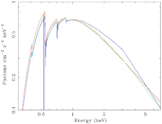
Intrinsic models with Galactic absorption only, in the energy range of 0.3–2.0 keV (Swift spectra extend to 10keV), simple power law (red), log-parabolic (green), and broken power law (blue). Below 1 keV, N, O, and Ne are the dominant absorption features.
3.3 Ionized IGM
In earlier studies which examined the hypothesis of absorption causing the observed soft X-ray spectral hardening, only an intrinsic host absorption or some discrete intervening neutral absorbers (DLAs, LLS, etc.) were considered. However, in blazars the host contribution is probably negligible, consistent with low levels of optical-UV extinction observed (Paliya et al. 2016). Further, strong intervening absorption by neutral absorbers (|${\it N}\small {\rm HI}$|) is too rare in blazar LOS to account for the observed curvature (e.g. Elvis et al. 2021; Cappi et al. 1997; Fabian et al. 2001; Page et al. 2005). Therefore, we omit any absorption contribution from the blazar host or low-column density intervening neutral Lyman absorbers (log(|${\it N}\small {\rm HI}) \lt 21$|) in our models. If there is a large known intervening absorber such as a galaxy (e.g. PKS 1830–211) or substantial DLA with log|$({\it N}\small {H\,I}) \gt 21$|, then it was included in the model using xspec ztbabs placed at the redshift of the intervening object. We note that it is possible that further unidentified individual strong absorbers may exist on the LOS to our sample which would then be included in the integrated |$\mathit {N}\small {\rm HXIGM}$| derived from the fits.
D21 examined different ionization models to represent diffuse IGM absorption including collisional ionized equilibrium models (CIE): hotabs (Kallman et al. 2009), ioneq (Gatuzz et al. 2015), and absori (Done et al. 1992), and photoionization equillibrim (PIE) model warmabs (Kallman et al. 2009). Absori allows one to have both ionization parameter and temperature as free parameters which would not occur in either pure PIE or CIE (Done 2010). In order to compare with CIE models, D21 froze the ionization parameter leaving temperature as a free parameter required for CIE scenarios. In earlier works on using tracers such as GRBs and blazars for IGM absorption, absori was generally used (e.g. Bottacini et al. 2010; Behar et al. 2011; Starling et al. 2013a, A18). While absori was the best model available when it was developed in 1992, it is not self-consistent, and is limited to 10 metals, all of which are fixed at solar metallicity except Fe (Done et al. 1992). D21 concluded that warmabs and hotabs are the most sophisticated of these models currently available, and the MCMC integrated probability plots were the most consistent with the steppar results. We followed their methodology for the modelling the IGM absorption. Initially, we fitted a sub-sample of 20 blazars with both PIE and CIE absorption separately as extreme scenarios where all the IGM absorption is either in the CIE or PIE phase. Consistently with D21, we found that similar results were obtained for both models and that it is not possible to conclude whether PIE or CIE is the better single model for the IGM at all redshift, though a combination is the most physically plausible scenario. Given the fact that similar results are obtained for both PIE and CIE models, we proceeded only with fitting CIE model hotabs. Therefore, the full models for each blazar in xspec language are (with the addition of ztbabs for known intervening objects):
tbabs*hotabs*logpar
or
tbabs*hotabs*bknpo
We model the IGM assuming a thin uniform plane-parallel slab geometry in thermal and ionization equilibrium. This simple approximation is generally used for a homogeneous medium (e.g. Savage et al. 2014; Nicastro et al. 2017; Khabibullin & Churazov 2019; Lehner et al. 2019). This slab is placed at half the blazar redshift as an approximation of the full LOS medium. The parameters ranges that were applied to the CIE models are taken from D21 and summarized in Table 3. We follow the same methodology as D21 in using hotabs and the IGM parameter range for IGM density, temperature and metallicity. D21 provides detail on hotabs that calculates the absorption due to neutral and all ionized species of elements with atomic number Z ≤ 30. Further, D21 clarifies that the fitting method uses the continuum total absorption to model plasma as opposed to fitting individual line absorption as the required resolution is not available currently in X-ray. As we are modelling and fitting the continuum curvature and not specific lines or edges specifically, scope for degeneracy occurs. In the D21 Supplementary material, transmission figures are gives to show the impact of changes in temperature, metallicity and redshift. In the cool IGM phases, typical metallicity is observed to be −4 < [X/H] < −2 (e.g. Schaye et al. 2003; Simcoe, Sargent & Rauch 2004; Aguirre et al. 2008). In the warmer phases including the WHIM, the metallicity has been observed to be higher [X/H] ∼ −1 (e.g. Danforth et al. 2016; Pratt et al. 2018). As we are modelling the LOS through the cool, warm and hot diffuse IGM, we will set the xspec metallicity parameter range following D21 as −4 < [X/H] < −0.7.
Upper and lower limits for the free parameters in the IGM models. Continuum parameters were also free parameters. The fixed parameters are Galactic log(|${\it N}\small {\rm HX}$|), the IGM slab at half the GRB redshift, and any known intervening object log(|${\it N}\small {\rm HX}$|).
| IGM parameter | range in xspec models |
|---|---|
| Column density | 19 ≤ log(|${\it N}\small {\rm HX}$|) ≤23 |
| Temperature | 4 ≤ log(T/K) ≤8 |
| Metallicity | −4 ≤ [X/H] ≤ −0.7 |
| IGM parameter | range in xspec models |
|---|---|
| Column density | 19 ≤ log(|${\it N}\small {\rm HX}$|) ≤23 |
| Temperature | 4 ≤ log(T/K) ≤8 |
| Metallicity | −4 ≤ [X/H] ≤ −0.7 |
Fig. 2 shows an example of the model components for the full LOS absorption using hotabs for IGM CIE absorption. The model example assumes a blazar at redshift z = 2.69, using a log-parabolic power law, hotabs for IGM CIE absorption, log|$({\it N}\small {\rm HXIGM}) = 22.28$|, [X/H] = −1.59, and log(T/K) = 6.2 for the IGM, and log(|${\it N}\small {\rm HX}) = 21.2$| for our Galaxy. The IGM CIE absorption curve is green, our Galaxy red and the total absorption from both components is the blue curve. In the model, the absorption lines are clearly visible. However, we would expect that these lines would not be detected due to instrument limitations and being smeared out over a large redshift range.
![Model components for the LOS absorption to a blazar using a log-parabolic power law, hotabs for IGM CIE absorption in the energy range of 0.3–2.0keV (Swift spectra extend to 10 keV). The model example is for a blazar at redshift z = 2.69, with log(${\it N}\small {\rm HXIGM}) = 22.28$, [X/H] = −1.59, and log(T/K) = 6.2 for the IGM, log(${\it N}\small {\rm HX}) = 21.2$ for our Galaxy. The IGM CIE absorption curve is green, our Galaxy red and the total absorption from both components is the blue curve.](https://oup.silverchair-cdn.com/oup/backfile/Content_public/Journal/mnras/508/2/10.1093_mnras_stab2597/1/m_stab2597fig2.jpeg?Expires=1750496954&Signature=HRwDNH3wTMeIPYjQYtyEBjAgnXyP7-OaqJE2UCOzd1DxYwrQQi3nywsXVHG3AoJ7M20FhPKfX8NpXb0CEn9kEXY0iiydsMZXy76g4pSp-rjcA9qzsKXYi9GUxcCsydQTj4Xs4IKmbnVodF8VdLziwRBTT56inZx60B1xelAM03suxAiG2aFpLS8RhzZEkjDNAR8Mbt8iSk51PGohkWhJge0og3GXOaDOKP6~OTG4wjizWUMjmhp0o37leqoWxjPKS0di-kbe28eVYhIcS-VOwig5RCbmj0bT117SmAzMiGtyxbHsql~TTc-tgL59ylYX6CQjrdzG4hZKsuO6QNHhmA__&Key-Pair-Id=APKAIE5G5CRDK6RD3PGA)
Model components for the LOS absorption to a blazar using a log-parabolic power law, hotabs for IGM CIE absorption in the energy range of 0.3–2.0keV (Swift spectra extend to 10 keV). The model example is for a blazar at redshift z = 2.69, with log(|${\it N}\small {\rm HXIGM}) = 22.28$|, [X/H] = −1.59, and log(T/K) = 6.2 for the IGM, log(|${\it N}\small {\rm HX}) = 21.2$| for our Galaxy. The IGM CIE absorption curve is green, our Galaxy red and the total absorption from both components is the blue curve.
4 SPECTRAL ANALYSIS RESULTS
In Section 4, we first discuss the impact of using different intrinsic blazar continuum models in Section 4.1, then give the results for IGM parameters for the full sample using the CIE IGM absorption model in Section 4.2. All spectral fits include tbabs for Galactic absorption.
4.1 Spectra fit improvements from alternative continuum models and IGM component
We show the fit results in Fig. 3 for J013126–100931 at redshift z = 3.51 as an example of typical results. We initially fitted a simple power law. The left-hand panel in Fig. 3 shows residuals at low energy with a Cstat of 273.24 for 330 deg of freedom (dof). We then tried both a log-parabolic and broken power law. The middle panel shows the fit with a broken power law that had a better result than both log-parabolic or simple power law, Cstat/dof = 262.88/328. An improved fit at soft energy can be seen. We then added a variable CIE IGM component to the broken power law while allowing the intrinsic parameters to also vary shown in the right-hand panel of Fig. 3. The spectral fit is improved compared with the Galactic absorbed broken law only model, with less low energy residual, Cstat/dof = 256.98/326. The left-hand and right-hand panels of Fig. 4 show the MCMC integrated probability results for |$\mathit {N}\small {\rm HXIGM}$| with temperature and broken power-law index (low energy), respectively. The red, grey and blue contours represent |$68{{\ \rm per\ cent}}, 90{{\ \rm per\ cent}}$| and |$95{{\ \rm per\ cent}}$| ranges for the two parameters, respectively. On the y-axis left-hand panel, log(T4/K) means that 0 is log(T/K) = 4. The contours in both plots and particularly |$\mathit {N}\small {\rm HXIGM}$| and the low energy power law provide reasonably tight ranges of parameter results at 2σ (|$95{{\ \rm per\ cent}}$| confidence).
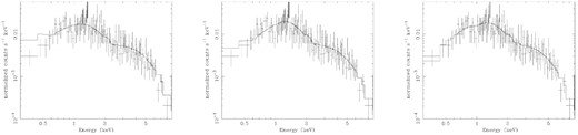
Impact of using different intrinsic curvature models and additional IGM absorption components for blazar J013126–100931. All fits include Galactic absorption. The left-hand panel is a simple power law. The middle panel is with a broken power law. The right-hand panel is a broken power law with a CIE IGM absorption component.
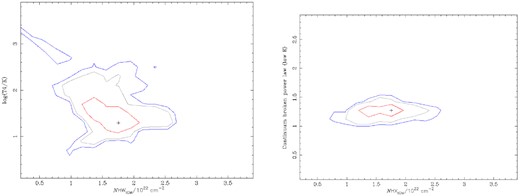
The left-hand and right-hand panels show the MCMC integrated probability results for J013126-100931 for |$\mathit {N}_{\small {\rm HXIGM}}$| with temperature and broken power law (low energy), respectively. The red, grey and blue contours represent |$68{{\ \rm per\ cent}}, 90{{\ \rm per\ cent}}$| and |$95{{\ \rm per\ cent}}$| confidence ranges for the two parameters, respectively. On the y-axis in the left-hand panel T4 means the log of the temperature is in units of 104 K.
4.2 IGM parameter results using a CIE IGM model
We note that in all cases, the addition of the absorption component improved the Cstat fit for all blazars in our sample indicating that the addition of the absorption component is required in the model. Overall, the best-fitting Cstat results were achieved using the IGM component with a log-parabolic power law (26/40 spectra). Only 6 blazars out of the sample with z > 1 (23), had a better fit with a broken power law. The continuum model fit favouring a log-parabolic or broken power law over a simple power law is consistent with prior studies (e.g. Bhatta, Mohorian & Bilinsky 2018; Sahakyan et al. 2020; Gaur 2020, A18). Modelling the IGM using hotabs for CIE with parameters |$\mathit {N}\small {\rm HXIGM}$|, Z and T free, results in |$\mathit {N}\small {\rm HXIGM}$| showing similar values and trend with redshift as the mean IGM density model. In the left-hand panel of Fig. 5, we show the results for |$\mathit {N}\small {\rm HXIGM}$| and redshift selecting the best fits from both log-parabolic and broken law (none were better with a simple power law). The right-hand panel of Fig. 5 are the results using the log-parabolic power law with the IGM component for comparison. Due to the differences between FSRQ (33/40 in our sample, blue) and BL Lac (red), we have plotted both categories coloured separately.
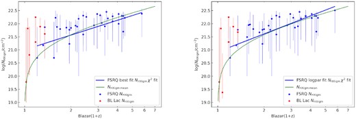
Results for the IGM |${\it N}\small {\rm HX}$| parameter and redshift using the CIE (hotabs) model. The error bars are reported with a |$90{{\ \rm per\ cent}}$| confidence interval. The green line is the simple IGM model using a mean IGM density. Left-hand panel is |${\it N}\small {\rm HX}$| and redshift selecting best Cstat results from the different power-law intrinsic models. Right-hand panel is the full sample with the IGM component and a log-parabolic power law only (best fit for 26/40).
Based on best-fitting results, a power-law fit to the |$\mathit {N}\small {\rm HXIGM}$| versus redshift trend for the FSRQ objects scales as (1 + z)1.8 ± 0.2, reduced χ2 = 1.69, (p-value = 0.0011, root mean square (rms) = 0.39). However, given that the FSRQ sample redshift includes blazars as low as z = 0.31, a linear χ2 fit is not appropriate as can be seen from the simple IGM curve. The mean hydrogen density using equation (1) at z = 0 from the FSRQ sample is n0 = (3.2 ± 0.5) × 10−7 cm−3. This is higher than the value of 1.7 × 10⁻⁷ cm−3 for the simple IGM model (green line in Fig. 5). Taking a sub-sample of FSRQ with z > 1.6, similar to the GRB sample in D21, gives n0 = (2.1 ± 0.2) × 10−7 cm−3. While noting that many of the error bars are large, jointly the blazars would support any model that is proximate to the χ2 fit that includes the mean IGM density curve. At low redshift, several blazars have higher |$\mathit {N}\small {\rm HXIGM}$| than the simple IGM model. This may be evidence of the CGM in both our Galaxy and the host galaxy providing a minimum column density. While there is no observed significant evolution in neutral hydrogen column density in the CGM, there is evidence of evolution in total hydrogen column density including the partially ionized hydrogen column (Fumagalli et al. 2016; Lehner et al. 2016). Models incorporating more advanced modelling for a warm/hot CGM component are needed to explore the relative contribution of the IGM and the host CGM to the observed absorption in blazars and GRBs (D21). Das et al. (2021) claim to have detected three distinct phases in our Galaxy CGM, with a hot phase having log(T/K) ∼7.5 and log|$(\mathit {N}\small {\rm HX}) \sim 21$|. The BL Lacs dominate the sample at very low redshift and the majority appear to have high |$\mathit {N}\small {\rm HXIGM}$| although with large error bars. This could be due to the overall model incorrectly describing the BL Lac spectra. The four BL Lac objects that most exceed the simple IGM curve are all high-energy peaked blazars, known as HBLs. These objects have their peak synchrotron humps at energies that can appear in soft X-ray. Therefore, we have excluded the BL Lac in our derivation of the mean hydrogen density at z = 0 and the χ2 fit for |$\mathit {N}\small {\rm HXIGM}$| versus redshift trend.
There is a large range in the fitted temperature 5.0 < log(T/K) <8.0, many with substantial error bars in the left-hand panel of Fig. 6. The mean temperature over the full redshift range is log(T/K) =6.1 ± 0.1. These values are consistent with the generally accepted WHIM. There is no apparent relation of temperature with redshift. It should be noted, however, that the fits are for the integrated LOS and not representative of any individual absorber temperature. Further, at high redshift, it is possible that the IGM comprises a cooler diffuse gas which is contributing to the absorption but not captured in this CIE model.
![Results for the IGM parameters and redshift using the CIE (hotabs) model best-fitting results from the various models. The error bars are reported with a $90{{\ \rm per\ cent}}$ confidence interval. Left-hand panel is temperature and redshift and right-hand panel is the [X/H] and redshift. We do not include a χ2 curve in the plots as the fit was poor due to a large scatter.](https://oup.silverchair-cdn.com/oup/backfile/Content_public/Journal/mnras/508/2/10.1093_mnras_stab2597/1/m_stab2597fig6.jpeg?Expires=1750496954&Signature=uEwsQNaE4HXRKaLaAWAkF4Uajx0dOujISsaD6xWitDBnS7tTkzB-UmXyeBdy5RtKyFZAdirERUUGnbX8cgpn-Z~0ab5BTA9rCMF1ucSJO8QLBbykms6-0uDTr4SzycWV59QtsAPUoJGdCVOJQwYoEuUOPKVzm~ffH1DdMmQ1OuZn9bJjIRrHonOFs0isPNbv1lqZQDQs9yocw6fNkALfYch97XXfmg78W3FUj3QkrgaSZ~qC8uRrANxVMCPw1zL8XQ-0~A4i2yQzayUrPuqruLq3KL2XvMGh6HoD4lK5XKGab0O6e8vfVg2ePKri5ZcHbORmr~oPQq1ZHczTV-Dosw__&Key-Pair-Id=APKAIE5G5CRDK6RD3PGA)
Results for the IGM parameters and redshift using the CIE (hotabs) model best-fitting results from the various models. The error bars are reported with a |$90{{\ \rm per\ cent}}$| confidence interval. Left-hand panel is temperature and redshift and right-hand panel is the [X/H] and redshift. We do not include a χ2 curve in the plots as the fit was poor due to a large scatter.
The right-hand panel of Fig. 6 shows no apparent relation of [X/H] with redshift. The mean metallicity over the full redshift range is [X/H] = −1.62 ± 0.04. Metallicity ranges from approximately [X/H] − 0.7 (0.2Z⊙) to [X/H] − 3 (0.001Z⊙) with one outlier. This is the BL Lac Mrk 501 at z = 0.03. The initial fitting went to the upper metallicity limit of [X/H] < −0.7. We increased the upper limit to solar and the best fit was with [X/H] = −0.08(0.8Z⊙). Our model may not be appropriate for this object.
In conclusion, with the caveats of low X-ray resolution, a CIE IGM component only and the slab model to represent to full LOS, there are reasonable grounds for arguing that the CIE model using hotabs is plausible for modelling the warm/hot component of the IGM at all redshifts. In all fits, the Cstat was better than best fits for models with only Galactic absorption. Our CIE IGM component had three free parameters, |$\mathit {N}\small {\rm HXIGM}$|, temperature and [X/H]. There is scope for degeneracy as we model the continuum curvature and not specific absorption features as set out in Section 3 and D21. While there was a large range in Cstat improvements across the sample, the average Cstat improvement for the full sample per free IGM parameter was 3.9, with 20 out of 40 blazars exceeding ΔCstat2 > 2.71. The model using a log-parabolic continuum model with a CIE IGM absorption appears to be more consistent with the simple IGM curve than the selected best fits from both log-parabolic and broken power laws. Overall, the results for |$\mathit {N}\small {\rm HXIGM}$| using either a log-parabolic or broken power law are statistically indistinguishable indicating that IGM component is independent. Our temperature and metallicity results are consistent with the expected values from simulations for a warm/hot phase. However, as noted in Section 3, initial trials with a warm photoionized IGM component gave similar results to a collisional ionized model. It is most likely that a combined model would be more physical, but testing this requires better data. We now test the robustness of the results in Section 5 and discuss the results further and compare with other studies in Section 7.
5 TESTS FOR ROBUSTNESS OF IGM PARAMETER RESULTS
There are several alternative potential explanations for the curvature seen in blazar spectra which may not be partly or wholly attributable to IGM absorption. |$\mathit {N}\small {\rm HXIGM}$| can be degenerate to some degree with spectral slope i.e. a harder spectrum slope can mimic higher |$\mathit {N}\small {\rm HXIGM}$| and vice versa. Further, blazars can be highly variable in flux and spectral slope. Finally, some fits were nearly indistinguishable in terms of visual spectra ratio and/or Cstat i.e. there may be a concern about an a priori assumption of IGM absorption. Accordingly, we examine our results from a number of perspectives to test their robustness.
5.1 Flux variability
Blazars are known to have spectral variability (associated with flux variability). The physical causes of such variability can involve many processes, such as particle acceleration, injection, cooling, and escape, which contain a number of known and unknown physical parameters (Gaur 2020). Also, a local absorber at the host can show variability, while an IGM absorber should not. An absorber that shows variability within a reasonable short time-frame cannot be on intergalactic length scales, and must therefore be attributed to the host, or to intrinsic variability of the source (Haim, Behar & Mushotzky 2019).
As noted in Section 2, we use co-added blazar spectra. To test for possible absorption variability and/or a relation between flux and spectral hardening, we selected a sub-sample of 8 blazars with a redshift range 0.86 ≤ z ≤ 3.26 as representative of the full sample. For each, we selected four different individual observations taken at different dates, with high counts but which showed different flux rates to the mean co-added rate. We used the log-parabolic model for all 8 blazars. Table A2 in the Appendix reports the Observation ID, count rate over the mean count rate, |$\mathit {N}\small {\rm HXIGM}$| and log-parabolic power law over the mean power law for each blazar observation.
In the left-hand panel of Fig. 7, we can see that there is no apparent relation between |$\mathit {N}\small {\rm HXIGM}$| and flux across all the observations, with a χ2 fit slope approximating zero (−0.09 ± 0.05). The blazars are individually colour-coded and there is no obvious relation between |$\mathit {N}\small {\rm HXIGM}$| and flux for any individual blazar apart from possibly 4C 38.41. From Table A2, we can see that all the individual results for |$\mathit {N}\small {\rm HXIGM}$| are consistent with the mean result within the errors for each blazar.

Testing for possible relation between |$\mathit {N}\small {\rm HXIGM}$| and flux variability or spectral slope for four individual observations from the sub-sample of eight blazars. Objects are colour-coded to enable comparison of individual blazar results as well as overall possible relations. Left-hand panel is |$\mathit {N}\small {\rm HXIGM}$| and flux variability given as count rate over mean count rate. Right-hand panel is |$\mathit {N}\small {\rm HXIGM}$| and individual log-parabolic power law/ mean power-law index for each object. The error bars are reported with a |$90{{\ \rm per\ cent}}$| confidence interval.
5.2 Column density and spectral slope degeneracy
Given the scope for degeneracy between |$\mathit {N}\small {\rm HXIGM}$| and spectral hardening, for the sub-sample of 8 blazars we checked for any relation between these two parameters using the same four individual observations for each. As previously noted, due to the large variability frequently observed in blazars, non-simultaneous observations are expected to show different states of the object. Therefore, the log-parabolic parameters and normalizations were allowed free to vary. In the right-hand panel of Fig. 7, we show the |$\mathit {N}\small {\rm HXIGM}$| using log-parabolic power law for all fits for the individual observations. There is no apparent relation between column density and power law indices with a χ2 slope fit of 0.10 ± 0.06. We again colour code each blazar and there is no apparent relation between |$\mathit {N}\small {\rm HXIGM}$| and power law index variability for any individual object.
Overall, our results are consistent with other studies (e.g. Haim et al. 2019, A18) which tested for a fixed absorber and noted that it did not change significantly across different observational times.
5.3 XMM–Newton spectra comparison
|$\mathit {XMM-Newton}$| has excellent low-energy response down to 0.15 keV, extreme sensitivity to extended emission, and large effective area facilitating analysis of the soft X-ray properties. We continued our robustness tests using XMM−Newton PN spectra for the same sub-sample of blazars with the exception of 4C 38.41 which was not available. We used the log-parabolic power law again with the CIE IGM component. We chose a selection of both individual spectra and co-added spectra as given in Table 2. We used the same energy range as Swift for consistent comparison (0.3–10 keV). We also separately fitted our model to an extended energy range of 0.16–13 keV given the excellent sensitivity of XMM−Newton over this range.
Table A3 in the Appendix reports the redshift, and |$\mathit {N}\small {\rm HXIGM}$| for Swift 0.3–10keV, XMM−Newton 0.3–10 keV and 0.16–13 keV, respectively, for each blazar. The values for |$\mathit {N}\small {\rm HXIGM}$| are consistent for each blazar within the errors. The left-hand panel of Fig. 8 shows |$\mathit {N}\small {\rm HXIGM}$| for Swift and both XMM−Newton fits for each blazar. To enable the error bars to be separately visible, we have very slightly changed the redshift of the three spectra for each object. All |$\mathit {N}\small {\rm HXIGM}$| are proximate to the simple IGM curve. We also plot the best χ2 fit for the Swift and both XMM−Newton energy ranges. The slopes of both the XMM−Newton fits are very similar with 0.3–10 keV being 2.3 ± 1.0 and 0.16–13 keV being 2.3 ± 0.4. The slope of the χ2 fit for Swift is slightly less at 1.6 ± 0.7. Overall, within the errors, the Swift and both XMM−Newton results are consistent.
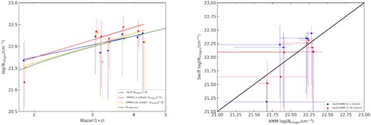
Comparing |$\mathit {N}\small {\rm HXIGM}$| and redshift results for Swift (blue), XMM−Newton (0.3–10keV)(red) and (0.16–13keV)(orange) from a sub-sample of seven blazars (varied slightly on the left-hand panel x-axis to enable error bar visibility). Left-hand panel is |$\mathit {N}\small {\rm HXIGM}$| and redshift. The green line is the simple IGM model using a mean IGM density. Right-hand panel is |$\mathit {N}\small {\rm HXIGM}$| for XMM−Newton on the x-axis (varied marginally for visibility) and Swift 0.3–10keV (blue) and 0.16–13keV (red) on the y-axis. The error bars are reported with a |$90{{\ \rm per\ cent}}$| confidence interval. The black line in the right-hand panel is parity.
In the right-hand panel of Fig. 8, we plot |$\mathit {N}\small {\rm HXIGM}$| for Swift on the x-axis and XMM−Newton 0.3–10 keV (blue) and 0.16–13keV (red) on the y-axis The black line in the right-hand panel is parity. We have varied the Swift|$\mathit {N}\small {\rm HXIGM}$| marginally to enable error bar visibility. All Swift and XMM − Newton data-points are proximate to the black parity line, with the possible exception of 3C 454.3 which has a reasonably higher |$\mathit {N}\small {\rm HXIGM}$| with Swift than XMM−Newton 0.3–10 keV, but consistent within the errors.
Fig. 9 show the MCMC integrated probability results for PKS0528+134 as a typical example of results for |$\mathit {N}\small {\rm HXIGM}$| and log-parabolic power law for Swift and XMM−Newton 0.3–10 keV, respectively. While the |$\mathit {N}\small {\rm HXIGM}$| best-fitting result is similar for both, due to the high resolution of XMM−Newton, the contours are much tighter.
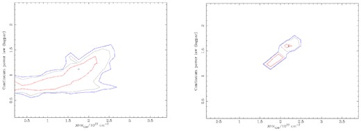
The left-hand and right-hand panels show the MCMC integrated probability results for PKS 0528+134 |$\mathit {N}_{\small {\rm HXIGM}}$| and log-parabolic power-law indices for Swift and XMM−Newton 0.3–10 keV, respectively. The red, grey, and blue contours represent |$68{{\ \rm per\ cent}}, 90{{\ \rm per\ cent}}$|, and |$95{{\ \rm per\ cent}}$| ranges.
Overall, our investigations demonstrate that our results are consistent for observations by both Swift and XMM−Newton. Further, they reinforce the findings from Section 5.2 that the IGM absorption results do not vary on a temporal basis.
5.4 Bulk comptonization
Some blazar spectra have a hump feature at soft X-rays, whose origin is still debated. Bulk Comptonization (BC) has been suggested as an explanation where cold electrons could up-scatter cooler extreme ultraviolet photons from the disk and/or BLR to soft X-ray energies (e.g. Sikora et al. 1994; Celotti, Ghisellini & Fabian 2007). This BC related excess emission over the blazar continuum would appear as a hump in soft X-ray. Depending on the energy peak of this hump, it could mimic or mask absorption. If the hump were to be in the region of ∼3 keV, the apparent deficit at softer energies can mimic absorption (and references therein Kammoun et al. 2018). This possible BC related feature has been modelled using a blackbody as a phenomenological representation (e.g Ricci et al. 2017).
Fig. 10 shows the spectrum of 3C 279 as an example of a FSRQ showing a second hump in soft X-ray where adding a blackbody component significantly improved the Cstat fit. All fits are with a broken power law that provided the best intrinsic curvature fit. The left-hand panel is with an IGM component (Cstat 992.1/933). The middle panel is with no IGM but an additional blackbody emission component (Cstat 917.06/934), where a slight visual improvement in fit can be seen at ∼0.6 keV. The right-hand panel is with both an IGM and blackbody component (Cstat 916.03/931).
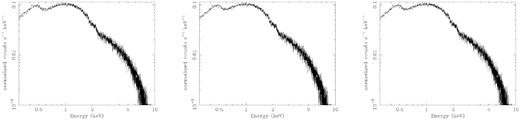
3C 279 as an example of FSRQ spectrum showing second hump in soft X-ray. All fits are with a broken power law, the best intrinsic curvature. The left-hand panel is with an IGM component. The middle panel is with a blackbody component. The right-hand panel is with both an IGM absorption component and a blackbody.
10 out of 40 in our blazar sample had a second soft X-ray hump where the Cstat was similar for both an IGM or blackbody component, and showed an improvement in Cstat with both components included. There was a large range in Cstat improvement for the model with both the IGM and blackbody components for the 10 blazars, with the average Cstat improvement per additional free blackbody parameter being 8.3, and 8 out of 10 blazars exceeding ΔCstat2 > 2.71.
In 8/10, there was a reduction in |$\mathit {N}\small {\rm HXIGM}$| in the combined IGM and BC model ranging up to one dex. 2/10 objects showed increased |$\mathit {N}\small {\rm HXIGM}$| from |$100{{\ \rm per\ cent}} \,{\rm to}\, 180{{\ \rm per\ cent}}$|. Given this large impact on |$\mathit {N}\small {\rm HXIGM}$|, we replotted the |$\mathit {N}\small {\rm HXIGM}$| redshift relation omitting the 10 blazars possibly impacted by a BC component. In Fig. 11, we can see the clear |$\mathit {N}\small {\rm HXIGM}$| redshift relation remains. In fact the power law fit to the |$\mathit {N}\small {\rm HXIGM}$| versus redshift trend for the FSRQ objects scales as (1 + z)2.4 ± 0.2 (p-value = 0.01, rms = 0.36) compared to (1 + z)1.8 ± 0.2 from the full sample (Section 4). The hydrogen equivalent density at z = 0 is similar at n0 = (3.5 ± 0.7) × 10−7 cm−3. Without the BC component, 5/10 favoured a log-parabolic power law over a broken power law. When the blackbody component was added, this changed to 9/10 favouring a broken power law.

Results for the IGM |${\it N}\small {\rm HX}$| parameter and redshift omitting the 10 blazars where adding a bulk Comptonization component improved the fit. The error bars are reported with a |$90{{\ \rm per\ cent}}$| confidence interval. The green line is the simple IGM model using a mean IGM density.
Based on our investigations, it appears possible that in some cases BC could mimic absorption. On the other hand, depending on where the energy peak of the blackbody-like feature occurs, it could also mask actual absorption, appearing as an excess at soft X-ray. BC itself is still not generally accepted as the cause of this feature. The majority of our sample show improved fit statistics for an IGM component. Further, the clear |$\mathit {N}\small {\rm HXIGM}$| redshift relation remains with the BC impacted blazars removed from the sample.
6 COMBINED BLAZAR AND GRB SAMPLE ANALYSIS
In this section, we combine the GRB sample from D21 with our full Swift blazar sample in a multiple tracer analysis across a redshift range 0.03 ≤ z ≤ 6.3. In this paper, we used D21 results from their fits using hotabs for CIE IGM for consistency. D21 isolated the IGM LOS contribution to the total absorption for the GRBs by assuming that the GRB host absorption was equal to ionized corrected intrinsic neutral column estimated from the Lyα host absorption. They used a realistic host metallicity, dust corrected where available, in generating the host absorption model.
As can be seen in Fig. 12, our results for blazars for a power law fit to the |$\mathit {N}\small {\rm HXIGM}$| versus redshift trend scaling as (1 + z)1.8 ± 0.2 (best cstat fit) is consistent with the GRBs in D21 which scale as (1 + z)1.9 ± 0.2 over the extended redshift. In the left-hand panel of Fig. 12, we use the best Cstat fit results for blazars and in the right-hand panel the log-parabolic only continuum results, in combination with the D21 GRB sample. The slopes of the χ2 fits for GRB and blazar best cstat |$\mathit {N}\small {\rm HXIGM}$| versus redshift are aligned, but the slope for the blazars using log-parabolic continuum power law in combination with the GRBs slightly better traces the simple IGM density curve over the full redshift.
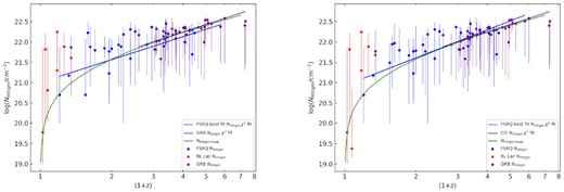
Results for the IGM |${\it N}\small {\rm HX}$| parameter and redshift using the combined GRB sample from D21 (purple) and our Blazar sample (FSRQ – blue and BL Lac – red) using the CIE (hotabs) model. The blue and purple lines are χ2 fits to the respective FSRQ and GRB samples. The error bars are reported with a |$90{{\ \rm per\ cent}}$| confidence interval. The green line is the simple IGM model using a mean IGM density. Left-hand panel is |${\it N}\small {\rm HX}$| and redshift selecting best Cstat results for blazars from all three power law intrinsic models. Right-hand panel is the full sample with the IGM component and a log-parabolic power law only (best fit for 26/40) for blazars.
The mean hydrogen density at z = 0 from the combined GRB and blazar samples is n0 = (2.2 ± 0.1) × 10−7 cm−3. This is marginally higher than the value of 1.7 × 10⁻⁷ cm−3 for the simple IGM model (green line in Fig 12) and for the GRB only sample in D21,n0 = (1.8 ± 0.1) × 10−7 cm−3. In Section 4, we reported the mean hydrogen density at z = 0 from the blazar FSRQ sample as n0 = (3.2 ± 0.5) × 10−7 cm−3. A possible explanation may be due to our assumption that there is no absorption in the blazar host due to the relativistic jet. In D21, it was also apparent that the lower redshift GRBs appeared to have higher |$\mathit {N}\small {\rm HXIGM}$| that the simple IGM curve. As speculated in Section 4.2, this may be a sign of CGM absorption from a hot phase as proposed by (Das et al. 2021). At higher redshift, the IGM contribution to |$\mathit {N}\small {\rm HXIGM}$| dominates any host contribution.
In Fig. 13, we show the combined GRB and blazar sample results for IGM temperature and metallicity. In the left-hand panel, we can see that there is no detectable overall trend with redshift. Some objects in the blazar sample, appear to have a higher maximum temperature than the GRB sample, up to log(T/K) ∼7.5. Das et al. (2021) have indicated that the Galaxy hot phase has a temperature of log(T/K) ∼7.5. The mean temperature over the full redshift range for the combined samples is log(T/K) =6.2 ± 0.1 under the assumption of a CIE scenario.
![IGM parameter results using the combined GRB sample from D21 (purple) and our Blazar sample (blue). The error bars are reported with a $90{{\ \rm per\ cent}}$ confidence interval. The left-hand panel is temperature and redshift and right-hand panel is the [X/H] and redshift. We do not include a χ2 curve in the temperature plot as the fit was poor due to a large scatter. In the right-hand panel, we show GRB and blazar combined χ2 curve for z > 0.9 showing a possible redshift relation above this redshift.](https://oup.silverchair-cdn.com/oup/backfile/Content_public/Journal/mnras/508/2/10.1093_mnras_stab2597/1/m_stab2597fig13.jpeg?Expires=1750496955&Signature=WerBl1nSBHMTCZSWLfTQtECXEHFski207BzWkAwP1p5UI92oHyr8H0VOAj1gsZz-FOzbNysNL-qFxp7-eOchXD5g7hjfVbbucdQiJBGHZo0VV8dZZ-lCPdrFFwgffzIbF1us5Ovy0DBsVu6J7mtRDPPgVvMjEwYFzmc3LQS8tCRIU0vHRwyV-msC6H2pLBS41BMtpxSbAKHrFQ2soh8e-9p8BMxnpwdglIAa61l3LS12Qund~JyADUpSqwFyarMxhvJE0NzMGDUcw8I9N9y3Bf2GdH1rKEiTjam6o01LCMq~ccoTtR5NToeh0kYPf92hrM-j4DrtZOYgeXbmnhvoQQ__&Key-Pair-Id=APKAIE5G5CRDK6RD3PGA)
IGM parameter results using the combined GRB sample from D21 (purple) and our Blazar sample (blue). The error bars are reported with a |$90{{\ \rm per\ cent}}$| confidence interval. The left-hand panel is temperature and redshift and right-hand panel is the [X/H] and redshift. We do not include a χ2 curve in the temperature plot as the fit was poor due to a large scatter. In the right-hand panel, we show GRB and blazar combined χ2 curve for z > 0.9 showing a possible redshift relation above this redshift.
In the right-hand panel of Fig. 13, we can see the IGM metallicity results for the combined GRB and blazar sample for 0.9 ≤ z ≤ 7. We omitted blazars with z < 0.9 as they showed very large scatter in best-fitting metallicity and with substantial errors. There appears to be a possible relation with redshift scaling as (1 + z)−2.9 ± 0.5 (orange χ2 line). The reduced χ2 is 1.9, with a p-value = 0.00014 and rms = 0.60, indicating a modestly statistical relation. Visually, the metallicity redshift relation, if any, is not clear, or may indicate that a linear model may not be appropriate. For the GRB only sample, D21 reported a power law fit to the [X/H] and redshift trend as (1 + z)−5.2 ± 1.0, ranging from [X/H] =−1 (Z = 0.1Z⊙) at z ∼ 2 to [X/H] ∼−3 (Z = 0.001Z⊙) at high redshift z > 4. They speculated that at low redshift, the higher metallicity warm-hot phase is dominant with Z ∼ 0.1 Z⊙, while at higher redshift the low metallicity IGM away from knots and filaments is dominant. In the combined blazar and GRB sample for z > 0.9, the possible redshift metallicity relation is less pronounced. While there is a large range in the lower error bars, some of the blazars at lower redshift have upper metallicity error bars approaching our upper limit of [X/H] = −0.7.
Overall, the IGM parameter results from our blazar sample are consistent with the GRB sample from D21. Therefore, the combined sample gives improved robustness to our reported results for the IGM.
7 DISCUSSION AND COMPARISON WITH OTHER STUDIES
The cause of spectral flattening seen in blazar spectra has been the subject of study and debate for some time. In early works, a cold local host absorber received favour (e.g. Cappi et al. 1997). Due to the low levels of optical-UV extinction seen in such blazars (e.g Elvis et al. 2021; Sikora et al. 1994), subsequent studies favoured an intrinsic curvature explanation with models including log-parabolic, broken power law and variations on this. We accommodated this element of intrinsic curvature by fitting our sample with best fit from a simple power law, log-parabolic and broken power law. Further, when adding the IGM component, we allowed all parameters to vary. In Section 5, we explored any possible relation between IGM absorption and both spectral flux and power-law hardening. No such relation was apparent.
Several studies have tentatively explored absorption scenarios, either neutral or a warm absorption component, as a minor part of their work, typically placing the absorber at the blazar redshift (e.g. Bottacini et al. 2010; Paliya et al. 2016; Ricci et al. 2017; Marcotulli et al. 2020; Haim et al. 2019). Bottacini et al. (2010) found they could not constrain their photo-ionized model parameter better than an upper limit. They used absori which is not as sophisticated as warmabs, the photoionized equivalent of our CIE model using hotabs. However, they reported that they found no evidence of absorption variability, consistent with our results. Ricci et al. (2017) used zxipcf, a photoionization model to test a scenario of a warm absorber in the blazar host with metallicity fixed to solar. They found that only a small number of fits improved with the added warm absorber component. This differs from our model where we allow both metallicity and temperature to vary, as solar metallicity is highly unlikely to occur in the diffuse IGM (e.g. Schaye et al. 2003; Aguirre et al. 2008; Shull et al. 2012, 2014), and we place the absorber at an intermediate redshift.
The relation between spectral flattening and redshift has been reported by several authors (e.g. Yuan et al. 2006; Behar et al. 2011). The hypothesis of discrete intervening absorbers (DLA, LLS, sLLS, etc.) has been investigated to explain this redshift relation (e.g. Wolf 1987). Several studies concluded that the absorption from such cool neutral intervening systems is rare and insufficient to be the cause of observed spectral curvature (and references therein Gianní et al. 2011), leaving the diffuse IGM as the alternative for non-localized intervening absorption.
Arguments against intervening IGM absorption are that intrinsic curvature is present in very low redshift blazars, or that absorption edges or lines are not observed in such very low redshift blazars (and references therein Watson & Jakobsson 2012), leading them to conclude that all the spectral flattening is due to intrinsic curvature at all redshifts. In general, most studies are focused on the blazar engine as the main or only cause of intrinsic curvature and leave out IGM absorption based on lack of significantly improved statistical fits. We would argue that it is highly likely that spectral curvature is due to a combination of both intrinsic factors as well as absorption, particularly at soft X-ray, given our findings for |$\mathit {N}{\small {\rm HXIGM}}$| and the redshift relation. If the apparent absorption was actually intrinsic to the blazars, then there would have to be some explanation of the relation to redshift which is absent.
Detection of the WHIM is proving very challenging due to very weak emission and absorption. Nicastro et al. (2018) claim to have observed the WHIM in absorption. However, with only 1 to 2 strong |$\rm{O\ \small {VII}}$| absorbers predicted to exist per unit redshift, the column densities they report are an order of magnitude lower than the simple IGM model, or the results for |$\mathit {N}{\small {\rm HXIGM}}$| reported by D21. Our results for the FSRQ sample |$\mathit {N}{\small {\rm HXIGM}}$| are consistent with the simple IGM model, though we note that many of the BL Lacs showed high |$\mathit {N}{\small {\rm HXIGM}}$|. Haim et al. (2019) searched for absorption lines as signals of localized IGM absorption in RBS 315 at z = 2.69, one of the brightest FSRQ known. They could find no such line absorption and concluded that, if blazar curvature is at least partly attributable to the IGM, it is not localized but smeared over redshift, consistent with our hypothesis and findings.
A18 is, to our knowledge, the only previous study that was dedicated to exploring the IGM as part of the cause of spectral flattening in blazar spectra, and to use blazars to investigate IGM properties. They used an absori based xpec model (igmabs) for the IGM absorption. They jointly fitted four blazars with IGM parameters of density, temperature and ionization tied together. They reported that excess absorption is the preferred explanation over intrinsic curvature and that it is related to redshift. They give an IGM average density of |$n_0 = 1.0^{+0.53}_{-0.72} \times 10^{-7}$| cm−3 and temperature log(T/K) |$= 6.45^{+0.51}_{-2.12}$|. Some caveats to their results are based on their solar metallicity assumption for the IGM and fixing the intrinsic power law parameters for some of their sample, which they adopted due to computational limits of their model which they noted would probably lead to upper limit measures for the IGM. Taking account of these factors, their results are broadly consistent with our results for IGM for n0 and T, but not for our mean IGM metallicity of [X/H] = −1.62 ± 0.04(∼ 0.02Z⊙). Their derived metallicity was |$Z_\rm {IGM} = 0.59^{+0.31}_{-0.42}Z\odot$|, obtained from the ratio of their n0 ∼ 1 result (based on solar metallicity) to the simple IGM model taken from (Behar et al. 2011) n0 = 1.7 × 10⁻⁷ cm−3. Campana et al. (2015) used simulations for intervening IGM absorption to AGN and GRBs. For GRBs, they reported log(T/K) ∼5 − 7. To calculate the metal column density of the intervening IGM material, 100 LOS to distant sources were used through a 100h−1 comoving Mpc Adaptive Mesh Refinement cosmological simulation (Pallottini, Ferrara & Evoli 2013). The contribution by each cell was summed, with an absorbing column density weighted for its effective temperature dependent value. Metallicity was obtained by requiring that only |$1{{\ \rm per\ cent}}$| of their GRB and AGN sample fall below the simulated hydrogen column density redshift curve. Their mean metallicity Z = 0.03Z⊙ is consistent with our results.
A18 combined their results for blazars with GRBs and AGN from other studies. However, all those studies were based on the assumption that all absorption in excess of our Galaxy was at the host redshift, neutral and at solar metallicity. Our combined tracer results in Section 6 are more realistic as we use the GRBs from D21 which more accurately isolate the IGM absorption assuming that the GRB host absorption was equal to ionized corrected intrinsic neutral column estimated from the Lyα host absorption. D21 also used more realistic host metallicity, dust corrected where available in generating the host absorption model as opposed to the conventional solar assumption.
8 CONCLUSIONS
We used blazars as tracers of the IGM with the main aim to probe the key parameters of column density, metallicity and temperature using a sophisticated software model for collisionally ionized plasma. We used co-added spectra from |$\mathit {Swift}$| for 40 blazars as our tracers with a redshift range of 0.03 ≤ z ≤ 4.7. Our focus is on FSRQ blazars, as they are available over a broad redshift range, and the rest-frame energy distribution of FSRQs is strongly peaked at low frequencies, below soft X-ray, unlike BL Lacs. We adopted a conservative approach to the blazar continuum model and use three different intrinsic power-law models. As blazars are thought to have a kpc-scale relativistic jet on our LOS, we excluded any host absorption in our models. We fixed the Galactic absorption to known values and attributed the excess to the IGM. We model the IGM assuming a thin uniform plane parallel slab geometry in CIE to represent a LOS through a homogeneous isothermal medium. We used xspec fitting with both the CIE IGM component and all power law parameters free to vary, and use steppar and MCMC to generate best fits to the blazar spectra.
We subjected our results to a number of robustness tests using a sub-sample: comparison of individual observation fit results with our co-added spectra for possible temporal absorption variability; testing for a relation between column density and flux; investigating spectral slope degeneracy with column density; comparing results from using XMM−Newton with energy range of 0.3–10 keV (as for Swift) and 0.16–13keV; and exploring the impact of using a blackbody like additional component to represent bulk comptonization that could mimic absorption.
Finally, we combined our sample with the GRB sample from D21 to report results for an extended redshift range using the two different types of tracers.
Our main findings and conclusions are:
the best-fitting Cstat results for our blazar sample were achieved using an IGM component with a log-parabolic power law (26/40 spectra) and appear to be more consistent with the simple model IGM curve than the selected best fits from both log-parabolic and broken power law.
Using blazars to model the IGM as being in highly ionized collisional equilibrium with free parameters for density, temperature, and metallicity (as well as continuum parameters) appears to give plausible IGM property results. A power-law fit to |$\mathit {N}\small {\rm HXIGM}$| versus redshift trend for the FSRQ objects scales as (1 + z)1.8 ± 0.2. The mean hydrogen density at z = 0 from the FSRQ sample is n0 = (3.2 ± 0.5) × 10−7 cm−3, higher than the value of 1.7 × 10⁻⁷ cm−3 for the simple IGM model (Fig 5). Nearly all blazar fits are proximate to both the χ2 fit and mean IGM density curve.
At low redshift, several blazars have higher |$\mathit {N}\small {\rm HXIGM}$| than the simple IGM model. BL Lacs dominate the sample at very low redshift and the majority appear have high fitted |$\mathit {N}\small {\rm HXIGM}$|. This may be due to CGM absorption.
The IGM temperature range is 5.0 < log(T/K) <8.0, with no apparent redshift relation in the left-hand panel of Fig. 6. The mean temperature over the full redshift range is log(T/K) =6.1 ± 0.1. These values are consistent with the generally accepted WHIM range indicating that very highly ionized metals are plausible absorbers over the LOS.
The right-hand panel of Fig. 6 shows no apparent relation of [X/H] with redshift (however, see Section 6 for possible metallicity redshift relation using combined blazar and GRB samples). The mean metallicity over the full redshift range is [X/H] = −1.62 ± 0.04(Z ∼ 0.02). Metallicity ranges from [X/H] − 0.7 (0.2Z⊙) to [X/H] − 3 (0.001Z⊙) with one outlier.
There was a large range in Cstat improvements across the sample, with the average Cstat improvement per free IGM parameter of 3.9. In our models the IGM contributes substantially to the total absorption seen in blazar spectra, and it rises with redshift. We provide evidence that a complete blazar model should also account for absorption by intervening IGM material.
In left-hand panel of Fig. 7, there is no apparent relation between |$\mathit {N}\small {\rm HXIGM}$| and flux across all the observations. All the individual results for |$\mathit {N}\small {\rm HXIGM}$| for each blazar are consistent with the mean result within the errors (Table A2).
There is no apparent relation between column density and power-law index. Further, there was no temporal variation in IGM parameter results per blazar using observations over time.
For Swift 0.3–10 keV, XMM−Newton 0.3–10 keV and 0.16–13 keV, respectively, the values for |$\mathit {N}\small {\rm HXIGM}$| using log-parabolic power laws are consistent for each blazar within the errors. All |$\mathit {N}\small {\rm HXIGM}$| are proximate to the simple IGM curve (the left-hand panel of Fig. 8). The slopes of both the XMM−Newton energy ranges are very similar. The slope of the χ2 fit for Swift is less steep but consistent with XMM−Newton within the error. The XMM−Newton results reinforce the findings that the IGM absorption results do not vary on a temporal basis.
Bulk Comptonization has been proposed as a cause of the hump feature at soft X-rays seen is some blazars. 10 out of 40 in our blazar sample had a second soft X-ray hump where the Cstat was similar for both an IGM or blackbody component. Based on our investigations, it appears possible that in some cases, BC could mimic absorption. On the other hand, depending on where the energy peak of the blackbody like feature occurs, it could also mask actual absorption, appearing as an excess at soft X-ray. We found that after omitting from the sample the blazars with possible BC, the |$\mathit {N}\small {\rm HXIGM}$| relation with redshift remains and the results are consistent with those from our full sample.
Combining our blazar sample with the GRB sample from D21 gives consistent results for the IGM properties over an extended redshift range from 0.03 ≤ z ≤ 6.3. The mean hydrogen density at z = 0 from the combined GRB and blazar samples is n0 = (2.2 ± 0.1) × 10−7 cm−3. This is marginally higher than the value of 1.7 × 10⁻⁷ cm−3 for the simple IGM model, but lower than the blazar only sample (n0 = (3.2 ± 0.1) × 10−7 cm−3), perhaps indicating that the blazar relativistic jet may not fully sweep out absorbing material in the host. Our blazar model assumes there is no host absorption which may be true for most FSRQ which are highly luminous, and hence probably more effective in removing host absorbing gas, but for the less luminous BL Lacs this may not completely happen. The mean temperature over the full redshift range is log(T/K) =6.1 ± 0.1, and the mean metallicity over the full redshift range is [X/H] = −1.62 ± 0.04(Z ∼ 0.02). These values are consistent with the generally accepted WHIM range indicating that very highly ionized metals are plausible absorbers over the LOS. There was no apparent temperature redshift relation. However, we found a possible relation for metallicity and redshift to be (1 + z)−2.9 ± 0.5.
This study is based on observations of blazar X-ray spectra, and provides results on the IGM parameters. The combination of blazars with the GRB sample gives consistent and more robust results for the IGM properties by using multiple tracer types. The IGM property constraints will only be validated when observations are available from instruments with large effective area, high-energy resolution, and a low-energy threshold in the soft X-ray energy band (e.g. Athena). We will continue our IGM exploration using other tracers in an upcoming paper and will combine the future results with those from this paper, D21 and D20.
ACKNOWLEDGEMENTS
We thank the anonymous referee for useful comments and suggestions. This work made use of data supplied by the UK Swift Science Data Centre at the University of Leicester; XMM–Newton, an ESA science mission with instruments and contributions directly funded by ESA member states and NASA. SLM also acknowledges support from STFC (ST/P000541/1). This project has received funding from the European Research Council (ERC) under the European Union’s Horizon 2020 research and innovation programme (grant no. 757535) and by Fondazione Cariplo (grant no. 2018-2329).
DATA AVAILABILITY
Supplementary data including spectra fit, parameter results for the continuum models and IGM, and MCMC integrated probability plots are available on request. Please contact Tony Dalton. Swift spectral data for blazars are available from https://www.swift.ac.uk/2SXPS.
Footnotes
Throughout this paper, logarithmic column densities are expressed in units of cm−2.
REFERENCES
APPENDIX: TABLES REPORTING FIT RESULTS FOR THE MAIN BLAZAR SAMPLE AND SUB-SAMPLES
Swift blazar sample. For each blazar, the columns give the name, type, redshift, IGM and continuum best cstat fitted parameter results: |$\mathit {N}\small {\rm HXIGM}$|, [X/H], temperature, log parabolic power law and β, or broken power law low-energy power law (PO1), energy break (Eb), and high-energy PO2, Cstat/dof.
| Blazar | Type | z | log|$\big(\frac{\mathit {N}\small {\rm HXIGM}}{\textrm {cm}^{-2}}\big)$| | [X/H] | log|$(\frac{\textrm {T}}{ K})$| | PO or PO1 | β or Eb | PO2 | Cstat/dof |
|---|---|---|---|---|---|---|---|---|---|
| Mrk 501 | BL Lac | 0.03 | |$19.78^{+2.07}_{-0.78}$| | |$-0.08^{+0.06}_{-0.07}$| | |$6.77^{+0.41}_{-0.17}$| | |$1.92^{+0.06}_{-0.05}$| | |$0.23^{+0.14}_{-0.16}$| | 474.61/525 | |
| PKS 0521−365 | BL Lac | 0.06 | |$21.82^{+0.40}_{-1.82}$| | |$-0.70^{+0.70}_{-0.19}$| | |$7.08^{+0.81}_{-0.05}$| | |$1.47^{+0.03}_{-0.03}$| | |$0.15^{+0.05}_{-0.08}$| | 752.59/759 | |
| BL Lac | BL Lac | 0.07 | |$20.81^{+1.07}_{-0.77}$| | |$-2.99^{+2.10}_{-0.05}$| | |$4.98^{+0.12}_{-0.01}$| | |$1.39^{+0.05}_{-0.06}$| | |$2.01^{+0.17}_{-0.23}$| | |$1.73^{+0.03}_{-0.04}$| | 874.68/917 |
| 1ES 0347−121 | BL Lac | 0.18 | |$21.30^{+0.90}_{-0.70}$| | |$-1.60^{+0.90}_{-0.70}$| | |$5.72^{+2.16}_{-0.56}$| | |$1.97^{+0.18}_{-0.11}$| | |$0.05^{+0.15}_{-0.21}$| | 375.95/443 | |
| 1ES 1216+304 | BL Lac | 0.18 | |$22.25^{+0.04}_{-0.79}$| | |$-2.92^{+1.25}_{-0.04}$| | |$5.46^{+1.50}_{-0.05}$| | |$1.54^{+0.06}_{-0.02}$| | |$0.65^{+0.03}_{-0.03}$| | 681.87/724 | |
| 4C +34.47 | FSRQ | 0.21 | |$20.70^{+1.19}_{-0.70}$| | |$-1.01^{+0.01}_{-0.91}$| | |$6.57^{+1.20}_{-0.93}$| | |$1.60^{+0.10}_{-0.06}$| | |$-0.15^{+0.08}_{-0.14}$| | 531.50/539 | |
| 1ES 0120+340 | BL Lac | 0.27 | |$21.89^{+0.34}_{-0.74}$| | |$-1.00^{+0.25}_{-0.75}$| | |$7.25^{+0.69}_{-0.23}$| | |$1.71^{+0.03}_{-0.03}$| | |$0.24^{+0.06}_{-0.06}$| | 589.57/698 | |
| S50716+714 | FSRQ | 0.31 | |$21.18^{+0.15}_{-0.01}$| | |$-2.00^{+0.20}_{-0.00}$| | |$5.11^{+0.15}_{-0.01}$| | |$1.87^{+0.03}_{-0.10}$| | |$0.13^{+0.11}_{-0.04}$| | 824.04/822 | |
| PKS 1510−089 | FSRQ | 0.36 | |$21.87^{+0.24}_{-0.12}$| | |$-1.82^{+0.64}_{-0.88}$| | |$5.14^{+0.42}_{-0.11}$| | |$2.10^{+0.20}_{-0.47}$| | |$0.98^{+0.10}_{-0.06}$| | |$1.33^{+0.02}_{-0.03}$| | 868.77/922 |
| J1031+5053 | BL Lac | 0.36 | |$21.63^{+0.54}_{-0.91}$| | |$-1.13^{+0.06}_{-0.08}$| | |$5.00^{+0.18}_{-0.05}$| | |$3.95^{+0.01}_{-1.42}$| | |$0.81^{+0.11}_{-0.11}$| | |$2.23^{+0.04}_{-0.11}$| | 463.45/525 |
| 3C 279 | FSRQ | 0.54 | |$20.70^{+1.37}_{-0.04}$| | |$-2.99^{+0.85}_{-0.01}$| | |$5.20^{+0.27}_{-0.04}$| | |$1.49^{+0.01}_{-0.02}$| | |$2.64^{+0.19}_{-0.26}$| | |$1.66^{+0.03}_{-0.03}$| | 992.21/933 |
| 1ES 1641+399 | FSRQ | 0.59 | |$22.23^{+0.27}_{-0.33}$| | |$-0.86^{+0.13}_{-0.96}$| | |$7.60^{+0.37}_{-0.21}$| | |$1.59^{+0.04}_{-0.03}$| | |$2.79^{+0.62}_{-0.37}$| | |$1.74^{+0.81}_{-0.47}$| | 681.57/739 |
| PKS 0637−752 | FSRQ | 0.64 | |$21.88^{+0.50}_{-0.97}$| | |$-1.50^{+0.74}_{-1.03}$| | |$6.40^{+1.50}_{-0.87}$| | |$2.08^{+0.31}_{-0.24}$| | |$1.10^{+0.33}_{-0.29}$| | |$1.63^{+0.09}_{-0.08}$| | 535.08/629 |
| PKS 0903−57 | FSRQ | 0.70 | |$21.80^{+0.54}_{-0.34}$| | |$-2.70^{+0.90}_{-0.30}$| | |$5.20^{+2.15}_{-0.26}$| | |$0.54^{+0.20}_{-0.18}$| | |$1.09^{+0.28}_{-0.24}$| | 371.01/433 | |
| 3C 454.3 | FSRQ | 0.86 | |$21.85^{+0.30}_{-0.24}$| | |$-2.92^{+0.28}_{-0.08}$| | |$5.03^{+0.22}_{-0.03}$| | |$1.29^{+0.03}_{-0.03}$| | |$2.30^{+0.18}_{-0.03}$| | |$1.54^{+0.03}_{-0.03}$| | 935.16/926 |
| PKS 1441+25 | FSRQ | 0.94 | |$21.77^{+0.33}_{-1.17}$| | |$-1.80^{+0.96}_{-0.43}$| | |$5.18^{+2.62}_{-0.11}$| | |$2.15^{+0.26}_{-0.16}$| | |$-0.03^{+0.29}_{-0.33}$| | 360.76/412 | |
| 4C +04.42 | FSRQ | 0.97 | |$21.23^{+0.68}_{-0.75}$| | |$-0.90^{+0.15}_{-0.95}$| | |$5.08^{+2.25}_{-0.07}$| | |$1.53^{+0.15}_{-0.24}$| | |$-0.30^{+0.30}_{-0.15}$| | 505.29/537 | |
| PKS 0208+512 | FSRQ | 1.00 | |$21.84^{+0.23}_{-0.11}$| | |$-1.13^{+0.07}_{-0.37}$| | |$6.65^{+0.15}_{-0.17}$| | |$1.60^{+0.02}_{-0.06}$| | |$3.28^{+0.35}_{-0.12}$| | |$1.84^{+0.02}_{-0.06}$| | 575.64/668 |
| PKS 1240−294 | FSRQ | 1.13 | |$21.93^{+0.22}_{-0.98}$| | |$-0.99^{+0.27}_{-0.90}$| | |$5.53^{+1.93}_{-0.34}$| | |$1.90^{+0.23}_{-0.75}$| | |$-0.31^{+0.84}_{-0.26}$| | 307.68/374 | |
| PKS 1127−14 | FSRQ | 1.18 | |$21.89^{+0.21}_{-0.98}$| | |$-1.51^{+0.75}_{-0.79}$| | |$5.00^{+0.16}_{-0.18}$| | |$2.37^{+1.59}_{-0.75}$| | |$0.59^{+0.27}_{-0.25}$| | |$1.41^{+0.05}_{-0.06}$| | 649.40/702 |
| NRAO 140 | FSRQ | 1.26 | |$22.19^{+0.15}_{-2.19}$| | |$-1.22^{+0.50}_{-0.78}$| | |$7.23^{+0.70}_{-0.80}$| | |$1.11^{+0.12}_{-0.08}$| | |$0.36^{+0.09}_{-0.17}$| | 724.79/696 | |
| OS 319 | FSRQ | 1.40 | |$21.59^{+0.51}_{-0.65}$| | |$-0.81^{+0.02}_{-0.40}$| | |$5.87^{+0.42}_{-0.08}$| | |$1.86^{+0.11}_{-0.41}$| | |$0.20^{+0.31}_{-0.14}$| | 366.43/384 | |
| PKS 2223−05 | FSRQ | 1.40 | |$22.31^{+0.18}_{-1.13}$| | |$-0.85^{+0.01}_{-1.30}$| | |$7.27^{+0.61}_{-1.39}$| | |$1.42^{+0.19}_{-0.09}$| | |$0.28^{+0.13}_{-0.32}$| | 433.27/484 | |
| PKS 2052−47 | FSRQ | 1.49 | |$22.26^{+0.17}_{-1.30}$| | |$-1.47^{+0.73}_{-0.93}$| | |$7.20^{+0.74}_{-0.98}$| | |$1.33^{+0.13}_{-0.11}$| | |$0.20^{+0.18}_{-0.21}$| | 374.12/451 | |
| 4C 38.41 | FSRQ | 1.81 | |$21.94^{+0.27}_{-0.96}$| | |$-0.76^{+0.04}_{-1.20}$| | |$7.22^{+0.16}_{-0.45}$| | |$1.37^{+0.03}_{-0.03}$| | |$0.17^{+0.04}_{-0.06}$| | 806.01/804 | |
| PKS 2134+004 | FSRQ | 1.93 | |$22.37^{+0.05}_{-1.32}$| | |$-1.59^{+0.84}_{-0.64}$| | |$7.32^{+0.07}_{-1.64}$| | |$1.45^{+0.16}_{-0.12}$| | |$0.25^{+0.16}_{-0.27}$| | 886.53/418 | |
| PKS 0528+134 | FSRQ | 2.06 | |$22.32^{+0.08}_{-0.64}$| | |$-1.60^{+0.47}_{-0.80}$| | |$6.92^{+0.25}_{-1.43}$| | |$0.88^{+0.33}_{-0.27}$| | |$1.59^{+0.28}_{-0.14}$| | |$1.52^{+0.08}_{-0.07}$| | 728.89/760 |
| 1ES 0836+710 | FSRQ | 2.17 | |$22.03^{+0.30}_{-0.11}$| | |$-2.38^{+1.26}_{-0.12}$| | |$5.18^{+1.80}_{-0.30}$| | |$1.15^{+0.03}_{-0.06}$| | |$2.15^{+0.15}_{-0.46}$| | |$1.35^{+0.03}_{-0.04}$| | 972.76/912 |
| PKS 2149+306 | FSRQ | 2.35 | |$22.11^{+0.12}_{-0.21}$| | |$-1.08^{+0.34}_{-0.39}$| | |$6.40^{+0.37}_{-0.49}$| | |$2.13^{+0.42}_{-0.66}$| | |$1.02^{+0.15}_{-0.12}$| | |$1.27^{+0.03}_{-0.06}$| | 858.87/825 |
| J1656−3302 | FSRQ | 2.40 | |$22.35^{+0.12}_{-0.03}$| | |$-0.72^{+0.02}_{-0.98}$| | |$7.19^{+0.65}_{-0.42}$| | |$0.12^{+0.46}_{-0.02}$| | |$1.50^{+0.62}_{-0.26}$| | |$1.36^{+0.13}_{-0.33}$| | 438.94/528 |
| PKS 1830−211a | FSRQ | 2.50 | |$22.20^{+0.10}_{-0.81}$| | |$-0.99^{+0.32}_{-0.55}$| | |$6.88^{+0.93}_{-1.84}$| | |$0.64^{+0.29}_{-0.23}$| | |$0.46^{+0.18}_{-0.25}$| | 784.65/858 | |
| TXS0222+185 | FSRQ | 2.69 | |$22.28^{+0.14}_{-0.96}$| | |$-1.59^{+0.64}_{-0.81}$| | |$7.00^{+0.88}_{-1.61}$| | |$0.99^{+0.18}_{-0.15}$| | |$0.36^{+0.15}_{-0.15}$| | 699.61/676 | |
| PKS 0834−20 | FSRQ | 2.75 | |$22.30^{+0.22}_{-0.74}$| | |$-0.95^{+0.22}_{-0.91}$| | |$7.03^{+0.73}_{-0.55}$| | |$0.88^{+0.40}_{-0.45}$| | |$0.54^{+0.47}_{-0.44}$| | 320.97/395 | |
| TXS0800+618 | FSRQ | 3.03 | |$22.37^{+0.06}_{-1.22}$| | |$-1.85^{+0.83}_{-0.54}$| | |$6.40^{+1.30}_{-1.98}$| | |$1.77^{+0.34}_{-0.80}$| | |$-0.61^{+0.87}_{-0.36}$| | 297.99/354 | |
| PKS 0537−286 | FSRQ | 3.10 | |$22.21^{+0.07}_{-1.02}$| | |$-2.99^{+2.21}_{-0.15}$| | |$5.13^{+2.65}_{-0.21}$| | |$1.16^{+0.13}_{-0.12}$| | |$0.04^{+0.16}_{-0.14}$| | 620.60/681 | |
| PKS 2126−158 | FSRQ | 3.27 | |$22.30^{+0.08}_{-1.38}$| | |$-2.30^{+1.54}_{-0.40}$| | |$5.51^{+1.60}_{-1.07}$| | |$1.10^{+0.15}_{-0.15}$| | |$0.34^{+0.18}_{-0.15}$| | 732.26/721 | |
| S50014+81 | FSRQ | 3.37 | |$21.70^{+0.76}_{-0.13}$| | |$-2.98^{+0.94}_{-0.00}$| | |$6.82^{+1.02}_{-1.62}$| | |$1.09^{+0.15}_{-0.11}$| | |$0.44^{+0.15}_{-0.18}$| | 492.23/582 | |
| J064632+445116 | FSRQ | 3.39 | |$22.45^{+0.09}_{-0.32}$| | |$-1.64^{+0.73}_{-0.66}$| | |$7.41^{+0.56}_{-1.35}$| | |$1.44^{+0.18}_{-0.17}$| | |$5.10^{+2.82}_{-1.20}$| | |$3.07^{+0.61}_{-1.65}$| | 289.92/309 |
| J013126−100931 | FSRQ | 3.51 | |$22.22^{+0.16}_{-0.69}$| | |$-1.37^{+0.34}_{-0.63}$| | |$5.06^{+2.53}_{-0.89}$| | |$1.24^{+0.28}_{-0.59}$| | |$0.01^{+0.65}_{-0.32}$| | 256.98/326 | |
| B3 1428+422 | FSRQ | 4.70 | |$22.51^{+0.01}_{-0.87}$| | |$-2.80^{+1.76}_{-0.09}$| | |$5.33^{+2.44}_{-1.09}$| | |$1.76^{+0.34}_{-0.80}$| | |$-0.63^{+1.04}_{-0.40}$| | 249.06/286 |
Intervening galaxy at z = 0.89 with |$\mathit {N}\small {\rm HX} = 1.94 \times 10^{22}$| included in fitting using ztbabs.
Swift 2SXPS Catalogue sub-sample for individual observation comparison with co-added spectra results. For each blazar, the columns give Observation ID, redshift, count rate/mean count rate, fitted IGM |$\mathit {N}\small {\rm HXIGM}$| and log-parabolic power law/ mean power law.
| Blazar | Observation ID | z | |$\frac{\rm{count\ rate}}{\rm{mean\ rate}}$| | log|$\big(\frac{\mathit {N}\small {\rm HXIGM}}{\textrm {cm}^{-2}}\big)$| | |$\frac{\rm {logpar\,\,power-law}}{\rm {mean\,\,power-law}}$| |
|---|---|---|---|---|---|
| 3C 454.3 | Mean | 0.86 | 1.00 | |$21.67^{+0.41}_{-1.19}$| | 1.00 |
| 00035030001 | 0.86 | 2.65 | |$22.06^{+0.22}_{-0.25}$| | 0.96 | |
| 00030024001 | 0.86 | 4.69 | |$21.76^{+0.47}_{-0.98}$| | 0.91 | |
| 00030024002 | 0.86 | 2.96 | |$21.86^{+0.23}_{-1.16}$| | 1.05 | |
| 00035030005 | 0.86 | 3.53 | |$22.30^{+0.17}_{-1.07}$| | 0.98 | |
| PKS 2149-306 | Mean | 2.35 | 1.00 | |$21.90^{+0.28}_{-1.12}$| | 1.00 |
| 00031404001 | 2.35 | 0.73 | |$21.90^{+0.53}_{-0.76}$| | 1.11 | |
| 00031404015 | 2.35 | 1.15 | |$22.03^{+0.13}_{-0.06}$| | 0.93 | |
| 00035242001 | 2.35 | 0.93 | |$22.30^{+0.20}_{-0.92}$| | 1.68 | |
| 00031404013 | 2.35 | 1.30 | |$22.36^{+0.11}_{-1.16}$| | 0.89 | |
| PKS 2126-158 | Mean | 3.26 | 1.00 | |$22.30^{+0.08}_{-1.38}$| | 1.00 |
| 00036356001 | 3.26 | 0.92 | |$22.37^{+0.07}_{-0.27}$| | 1.45 | |
| 00036356003 | 3.26 | 0.92 | |$22.37^{+0.01}_{-1.30}$| | 1.19 | |
| 00036356004 | 3.26 | 0.88 | |$22.44^{+0.00}_{-1.32}$| | 1.11 | |
| 00036356002 | 3.26 | 0.96 | |$21.70^{+0.61}_{-0.70}$| | 1.17 | |
| PKS 0537-286 | Mean | 3.10 | 1.00 | |$22.21^{+0.07}_{-1.02}$| | 1.00 |
| 00035240001 | 3.10 | 0.93 | |$22.15^{+0.33}_{-0.33}$| | 1.04 | |
| 00035240002 | 3.10 | 0.95 | |$22.34^{+0.17}_{-0.60}$| | 0.91 | |
| 00036783001 | 3.10 | 1.25 | |$22.31^{+0.18}_{-0.67}$| | 1.10 | |
| 00030816005 | 3.10 | 1.15 | |$22.00^{+0.46}_{-0.40}$| | 1.22 | |
| 1ES 0836+710 | Mean | 2.17 | 1.00 | |$21.85^{+0.36}_{-0.98}$| | 1.00 |
| 00035385001 | 2.17 | 1.16 | |$21.90^{+0.39}_{-0.76}$| | 1.16 | |
| 00036376012 | 2.17 | 0.93 | |$22.32^{+0.12}_{-0.10}$| | 1.66 | |
| 00080399002 | 2.17 | 1.30 | |$22.27^{+0.09}_{-1.31}$| | 0.95 | |
| 00036376005 | 2.17 | 0.83 | |$22.04^{+0.39}_{-1.26}$| | 1.21 | |
| TXS 0222+185 | Mean | 2.69 | 1.00 | |$22.28^{+0.13}_{-0.96}$| | 1.00 |
| 00080243001 | 2.69 | 1.15 | |$22.26^{+0.09}_{-0.04}$| | 1.38 | |
| 00080243002 | 2.69 | 0.91 | |$22.40^{+0.08}_{-0.14}$| | 1.18 | |
| 00030794003 | 2.69 | 0.95 | |$22.34^{+0.14}_{-0.85}$| | 1.33 | |
| 00030794002 | 2.69 | 0.99 | |$22.27^{+0.16}_{-0.97}$| | 1.01 | |
| 4C 38.41 | Mean | 1.81 | 1.00 | |$21.94^{+0.22}_{-0.76}$| | 1.00 |
| 00036389050 | 1.81 | 1.23 | |$22.29^{+0.21}_{-1.29}$| | 1.20 | |
| 00036389059 | 1.81 | 2.14 | |$21.89^{+0.22}_{-0.64}$| | 0.95 | |
| 00032894004 | 1.81 | 1.84 | |$21.99^{+0.31}_{-0.33}$| | 1.37 | |
| 00036389052 | 1.81 | 1.16 | |$22.35^{+0.12}_{-0.92}$| | 0.97 | |
| PKS 0528+134 | Mean | 2.06 | 1.00 | |$22.23^{+0.14}_{-0.86}$| | 1.00 |
| 00035384002 | 2.06 | 1.63 | |$22.35^{+0.05}_{-1.05}$| | 0.44 | |
| 00035384003 | 2.06 | 2.12 | |$22.20^{+0.28}_{-1.60}$| | 1.80 | |
| 00035384005 | 2.06 | 2.16 | |$22.30^{+0.14}_{-1.12}$| | 1.30 | |
| 00035384006 | 2.06 | 2.58 | |$22.26^{+0.15}_{-0.17}$| | 2.81 |
XMM–Newton, 0.3–10 keV and 0.16–13 keV, and Swift sub-sample IGM column density results. For each blazar, the columns give Blazar name, redshift, fitted IGM |$\mathit {N}\small {\rm HXIGM}$| for Swift, XMM−Newton 0.3–10 keV and 0.16–13 keV, respectively.
| Swift 0.3–10 keV | XMM−Newton 0.3–10 keV | XMM−Newton 0.16–13 keV | ||
|---|---|---|---|---|
| Blazar | z | log|$\big(\frac{\mathit {N}\small {\rm HXIGM}}{\textrm {cm}^{-2}}\big)$| | log|$\big(\frac{\mathit {N}\small {\rm HXIGM}}{\textrm {cm}^{-2}}\big)$| | log|$\big(\frac{\mathit {N}\small {\rm HXIGM}}{\textrm {cm}^{-2}}\big)$| |
| 3C 454.3 | 0.86 | |$21.67^{+0.41}_{-1.19}$| | |$21.18^{+0.95}_{-0.57}$| | |$21.52^{+0.04}_{-0.12}$| |
| PKS2149−306 | 2.35 | |$21.90^{+0.28}_{-1.12}$| | |$22.18^{+0.05}_{-0.68}$| | |$22.09^{+0.19}_{-0.91}$| |
| PKS2126−158 | 3.26 | |$22.30^{+0.08}_{-1.38}$| | |$22.10^{+0.13}_{-1.40}$| | |$22.11^{+0.11}_{-1.62}$| |
| PKS0537−286 | 3.10 | |$22.21^{+0.07}_{-1.02}$| | |$22.35^{+0.02}_{-0.37}$| | |$22.26^{+0.09}_{-0.39}$| |
| 1ES0836+710 | 2.17 | |$21.85^{+0.36}_{-0.98}$| | |$22.23^{+0.17}_{-1.19}$| | |$21.64^{+0.37}_{-0.87}$| |
| TXS0222+185 | 2.69 | |$22.28^{+0.13}_{-0.96}$| | |$22.44^{+0.04}_{-0.08}$| | |$22.18^{+0.04}_{-0.09}$| |
| PKS0528+134 | 2.06 | |$22.23^{+0.14}_{-0.86}$| | |$22.34^{+0.07}_{-0.12}$| | |$22.31^{+0.08}_{-0.14}$| |
