


ABSTRACT
Quantifying tensions – inconsistencies amongst measurements of cosmological parameters by different experiments – has emerged as a crucial part of modern cosmological data analysis. Statistically significant tensions between two experiments or cosmological probes may indicate new physics extending beyond the standard cosmological model and need to be promptly identified. We apply several tension estimators proposed in the literature to the dark energy survey (DES) large-scale structure measurement and Planck cosmic microwave background data. We first evaluate the responsiveness of these metrics to an input tension artificially introduced between the two, using synthetic DES data. We then apply the metrics to the comparison of Planck and actual DES Year 1 data. We find that the parameter differences, Eigentension, and Suspiciousness metrics all yield similar results on both simulated and real data, while the Bayes ratio is inconsistent with the rest due to its dependence on the prior volume. Using these metrics, we calculate the tension between DES Year 1 3 × 2pt and Planck, finding the surveys to be in ∼2.3σ tension under the ΛCDM paradigm. This suite of metrics provides a toolset for robustly testing tensions in the DES Year 3 data and beyond.
1 INTRODUCTION
Two experiments are generally expected to agree, roughly within the reported errors, on the measured values of cosmological parameters. A disagreement between such measurements – a tension – may be a sign of a mistake in one or both analyses, of unaccounted-for systematic errors, or perhaps of new physics. A prominent historical example of such tensions in cosmology is the disagreement between a variety of measurements of the matter density Ωm in the 1980s and 1990s that was vigorously debated at the time (Peebles 1984; Efstathiou, Sutherland & Maddox 1990; Krauss & Turner 1995; Ostriker & Steinhardt 1995) and eventually turned out to be explained by the discovery of the accelerating universe (Riess et al. 1998; Perlmutter et al. 1999).
Presently, the discrepancy between the measurements of the Hubble constant using the distance ladder, |$H_0 = (74.03 \pm 1.42) {\, \rm km\, s^{-1}\, Mpc^{-1}}$| (Riess et al. 2019), and those from Planck, |$H_0 = (67.4 \pm 0.5) {\, \rm km\, s^{-1}\, Mpc^{-1}}$| (Planck Collaboration 2018), is much discussed, as it may be a harbinger of new physics. Similarly, recent measurements of the parameter combination1S8 ≡ σ8(Ωm/0.3)0.5 from large-scale structure by the Dark Energy Survey (DES; Abbott et al. 2018) and the Kilo Degree Survey (Asgari et al. 2020; Heymans et al. 2020) differ from the cosmic microwave background (CMB) estimates from the Planck satellite at ∼2–3σ significance. These Nσ quantifications of tension are generally understood to correspond to probabilities equivalent to 1D normal distribution, so that 1σ corresponds to 68 per cent confidence that the measurements are discrepant, 2σ corresponds to 95 per cent, etc.
The challenge is how to convert constraints from two data sets into such a probabilistic measure of tension between them. There exist a variety of methods to do this, which are being actively used in the community. While these tension metrics are expected to give consistent messages in cases where the two data sets obviously agree or disagree, in more marginal cases the differences amongst them – including how much they depend on an analysis’ choice of priors, assumptions of posterior Gaussianity, and the higher dimensional shape of the posterior – have the potential to alter the assessment of whether or not two data sets are in agreement.
In the lead-up to cosmological results expected from the analysis of DES year 1 to year 3 data (henceforth; simply Y3) and to inform other future cosmological analyses, we wish to provide a comprehensive characterization of how several proposed methods compare to one another. We also wish to confront these results with our intuition for what these metrics ought to be telling us about the agreement or disagreement between measurements. We specifically apply the methods to assess the consistency of DES and Planck. This paper complements two earlier analyses that test the consistency of probes within DES (Doux et al. 2020; Miranda, Rogozenski & Krause 2020).
These metrics serve only as diagnostics for whether there is tension, and not as a solution. If tension exists, it would indicate either unaccounted-for systematic effects in one or both experiments, or that the underlying model is inadequate to explain the data.
Our basic approach is to create a suite of simulated DES data sets with a controlled level of induced tension relative to the best-fitting Planck 2018 cosmology. We then apply a number of methods to quantify this synthetic tension and assess their performance. Finally, we apply the same tension metrics to quantify any tension between the published constraints from the first year of DES data (DES Y1) and the Planck 2015 and 2018 data sets.
The paper is structured as follows: we discuss the difficulties of tension estimation, and present the motivation of the present problem in Section 2. We then describe our methodology in Section 3. The different tension metrics studied in this paper are presented in Section 4. We show results on simulated DES data in Section 5, apply the tension metrics to DES Y1 in Section 6, and present our conclusions in Section 7.
2 MOTIVATION
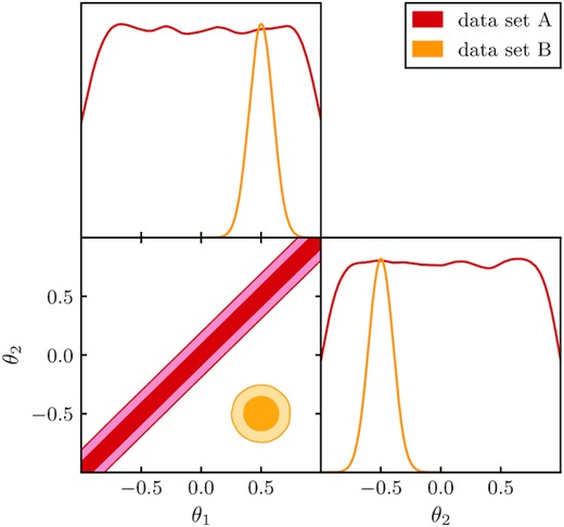
Toy model example of a set of 2D constraints, where the 1D projections hide the discrepancy between the two data sets. The darker and lighter shade correspond to the |$68{{\ \rm per\ cent}}$| and |$95{{\ \rm per\ cent}}$| confidence regions, respectively.
There is no unique, universally accepted method to quantify tension under these complicating circumstances. A variety of methods have been proposed, reviewed, and tested (Charnock, Battye & Moss 2017). Given this array of options, it is not obvious what the best choice is for a given analysis. In order to aid in this determination, in this paper, we will describe and study several of these methods in order to compare their performance when applied to DES data. In doing so, we distinguish between two kinds of tension:
Internal tensions, between different cosmological probes within one experiment (e.g. DES cosmic shear versus galaxy clustering within DES).
External tensions, between different experiments (e.g. DES versus Planck).
These must be treated differently because data-related systematic effects within the same experiment are often strongly correlated, necessitating use of more complex statistical tools when studying consistency. While our methodology can be applied to either type of tension, here we specifically apply it to the case of external tensions. In addition, we focus on quantifying the tension between the large-scale structure measurements (via the combination of galaxy clustering, galaxy–galaxy lensing and cosmic shear, or often referred to as the “3 × 2pt” probes) from DES, and the CMB measurements from Planck. Internal tension will be separately and additionally studied in Doux et al. (2020) using Posterior Predictive Distributions (PPDs; Gelman et al. 2004), which allow us to quantify tension in the presence of correlated systematic errors in the data, and to visualize the source of tension in the data vector. We do not consider the PPD in this work since it is not well suited to external tensions where there are many parameters that the two data sets do not share.
The challenge of accurately quantifying tension starts to become apparent as we investigate the expected performance of the tension metrics. Naïvely, one might think that shifting one parameter by a controlled number of marginalized N standard deviations would imply that the tension in the full-dimensional space would also be Nσ; or in other words, that the amount of tension in the full, N-dimensional space is equal to the tension projected2 to the original dimension. However, this is not the case, because of two effects:
Marginalization can hide tension that can only be seen in higher dimensions. This is caused by the fact that marginalization leads to loss of information. This means that the full-dimensional tension can be larger than that inferred by looking at 1D distributions of the parameters. This is illustrated with the simple 2D example shown in Fig. 1: there are two parameters θ1 and θ2, and they are highly correlated as measured by experiment 1, but largely uncorrelated as measured by experiment 2. Because experiment 1 determines both parameters separately quite poorly, 1D plots of the posterior show general agreement between measurements of the two experiments. Yet the 2D plot shows that the two contours are significantly separated. This is because the well-measured combination of θ1 and θ2 significantly differs between experiment 1 and experiment 2.
Relatedly, the number of dimensions of the problem also affects the inferred tension. The significance of a difference in parameter estimations between two experiments depends on the number of parameters constrained simultaneously by both experiments. Consider, for example, two experiments that measure the same parameter θ and obtain a 1D 3σ disagreement. The level of significance of this result is much higher if θ is the only parameter constrained by both experiments, than it is if the experiments also measure a hundred extra parameters, with no significant discrepancies between them. This common problem of the dilution of true tension with multiple comparisons is well known in statistics. For example, Heymans et al. (2020) report a ∼3σ tension with Planck in S8 alone, but a ∼2σ tension when considering the full multidimensional parameter space.
3 SETTING UP THE PROBLEM
The aim of this work is to compare and understand the performance of different metrics for measuring tension between DES and Planck constraints on cosmological parameters. If the two experiments report different values for some cosmological parameters, this might be an indicator that their results are not compatible. However, it is important to understand what this discrepancy means when considering the entire model. To do this, we use synthetic DES and Planck data sets that have been generated with different input cosmological parameters in order to produce varying levels of expected tension. By applying the various tension metrics to these synthetic data, we can study how they compare to one another and the known input parameter discrepancies. Note that we do not attempt to explain the origin of the possible incompatibility in cosmological parameters reported by two experiments.
We study tension in the context of the flat ΛCDM cosmological model. Our parameters are {Ωm, Ωb, H0, As, ns}, where Ωm and Ωb are the density parameters for matter and baryons, respectively; H0 is the Hubble constant; and As and ns are respectively the amplitude and slope of the primordial curvature power spectrum at a scale of k = 0.05 Mpc−1. We assume one massive and two massless neutrino species with the total mass equal to the minimum allowed by the oscillation experiments, mν = 0.06 eV. We do not vary the neutrino mass in our analysis in the simulated data sets, but we do in the reanalysis of tension between DES Y1 and Planck of Section 6, to be consistent with the DES Y1 3 × 2pt analysis choices (Krause et al. 2017). The data and prior choices are further described in Section A.
We use the CosmoSIS framework3 (Zuntz et al. 2015) to extract the best-fitting cosmological parameters from the Planck 2015 likelihood by sampling it using Nested Sampling (Skilling 2006), via the PolyChord algorithm4 (Handley, Hobson & Lasenby 2015a, b). From this chain, we infer the best-fitting values of the ΛCDM model parameters according to Planck data and use model predictions from these values to generate a baseline simulated DES-like 3 × 2pt data-vector under the Planck cosmology, henceforth referred to as the baseline cosmology. As previously mentioned, the simulated DES data are composed of galaxy clustering, cosmic shear, and galaxy–galaxy lensing correlation functions (Abbott et al. 2018).
3.1 Generating a priori tension
A convenient starting point in our analysis would be synthetically generated tension in two data sets, corresponding to data vectors generated at different values of cosmological parameters. Precisely how different these two sets of cosmological parameters are should be guided by some preliminary measure of tension. This starting point is henceforth referred to as the ‘a priori Gaussian tension’, and in this subsection, we provide a recipe to define it.
A shift in σ8 is obtained by changing the input value of As. Shifting Ωm, on the other hand, changes the history of structure growth and thereby σ8; we compensate for this collateral shift in σ8 by counter-shifting As. The DES constraints (shown in the Ωm–σ8 plane) from a representative subset of these shifted synthetic data are shown in Fig. 2.

Marginalized 2D posteriors for some of the simulated DES chains used in this work. The darker and lighter shades correspond to the |$68{{\ \rm per\ cent}}$| and |$95{{\ \rm per\ cent}}$| confidence regions, respectively.
Fig. 3 shows the distribution of shifted parameter combinations we describe above, as well as the baseline Planck + DES parameter constraints. Specifically, the contour shows the combined baseline Planck + DES constraints, while the markers show the best-fitting values of individual shifted DES-only constraints. We can immediately see that, in multiple dimensions, the tension that we attributed to a 1D shift is higher since Ωm and σ8 are correlated.
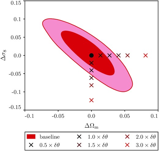
|$68 {{\ \rm per\ cent}}$| and |$95 {{\ \rm per\ cent}}$| confidence regions of the constraint on the differences in parameters as measured by DES and Planck, constructed as discussed in Section 3. The markers indicate the location of the synthetic input shifts. The corresponding a priori Gaussian tension is shown in Table 1.
The resulting evaluation of the a priori Gaussian tension is shown in Table 1. Here, the first column shows the parameter shift applied to DES data in the (Ωm, σ8) space, where each parameter is shifted by a half-integer multiple of its reported (marginalized) error. The second column shows the full-parameter-space tension calculated using Equation (4) as described above. Note that the ‘input shifts’ in Ωm lead to higher tension than those in σ8. This is because shifting Ωm while keeping σ8 fixed also leads to a shift in As, which increases the tension in the full-dimensional space.
Evaluation of a-priori Gaussian tension for controlled shifts in (σ8 and Ωm). The δθ by whose half-integer value we are shifting these parameters is referring to their respective 1D marginalized posterior as in equation (2). See equation (4) for the explanation how we convert these shifts into the “number of sigmas” in the full parameter space, shown in the second column.
| Evaluation of a priori Gaussian tension | |
|---|---|
| (Ωm, σ8) shift | full-par-space N-σ |
| |$\Delta \sigma _8 = -0.5\, \times \delta \sigma _8$| | |$0.02\, \sigma$| |
| |$\Delta \Omega _{\rm m} = +0.5\, \times \delta \Omega _{\rm m}$| | |$0.09\, \sigma$| |
| |$\Delta \sigma _8 = -1\, \times \delta \sigma _8$| | |$0.4\, \sigma$| |
| |$\Delta \Omega _{\rm m} = +1\, \times \delta \Omega _{\rm m}$| | |$1.0\, \sigma$| |
| |$\Delta \sigma _8 = -1.5\, \times \delta \sigma _8$| | |$1.1\, \sigma$| |
| |$\Delta \Omega _{\rm m} = +1.5\, \times \delta \Omega _{\rm m}$| | |$2.3\, \sigma$| |
| |$\Delta \sigma _8 = -2\, \times \delta \sigma _8$| | |$2.0\, \sigma$| |
| |$\Delta \Omega _{\rm m} = +2\, \times \delta \Omega _{\rm m}$| | |$3.8\, \sigma$| |
| |$\Delta \sigma _8 = -3\, \times \delta \sigma _8$| | |$3.7\, \sigma$| |
| |$\Delta \Omega _{\rm m} = +3\, \times \delta \Omega _{\rm m}$| | |$\gt 5 \, \sigma$| |
| |$\Delta \sigma _8 = -5\, \times \delta \sigma _8$| | |$\gt 5 \, \sigma$| |
| |$\Delta \Omega _{\rm m} = +5\, \times \delta \Omega _{\rm m}$| | |$\gt 5 \, \sigma$| |
Finally, let us note that the a priori tension, by its construction, does not contain stochastic noise, as it effectively measures the distance in the space of input cosmological parameters. This is in contrast with all of the tension metrics that we study below, which are applied to random realizations of data that do contain noise. The fact that the effectively noiseless input tension is being compared to tension measurements applied on noisy data are one reason why we do not expect a perfect match between the two. We will return to this point in Section 5.
4 TENSION METRICS
This section describes the tension metrics that we will be comparing in this work. Several metrics have been proposed for quantifying tension between cosmological data sets. In this work, we select a series of methods that we believe to be appropriate to our data, and which are distinct enough to highlight the strengths and failure modes of each metric. We separate the tension metrics into two subcategories, since while all methods aim to quantify tension between data sets, they answer slightly different questions:
Evidence-based methods seek to answer the question:
Given hypothesis H1: ‘The assumed model is capable of generating the data observed by both experiments’, and hypothesis H2: ‘The assumed model is not capable of generating the data observed by both experiments’, which hypothesis is preferred by the data under the assumed model’?
Parameter-space methods seek to answer the question:
What is the statistical significance of the differences between the posteriors for experiments A and B, within the parameter space analysed by both experiments?
All of the tension metrics that we consider solve the problems that we have discussed in Section 2 by considering all dimensions of parameter space. In addition, since they provide results in terms of probabilities, they are independent of the specific parametrizations that are used.
The remainder of this section describes these tension metrics. The results for these metrics will be shown in Section 5.
4.1 Bayesian evidence ratio
![Example of the prior-volume dependence of R. In amber and red are two Gaussians that are at a 3σ tension. The black dotted line is the prior (note that it is not normalized, to make it easier to visualize). When we use a uniform prior in the range [ − 10, 10] (left-hand panel), R is much smaller than one, which means the data sets are in tension. When we increase the prior to [ − 200, 200] (right-hand panel), R becomes greater than one, indicating agreement. This example, although extreme, illustrates a possible issue of the Bayes ratio as a tension metric.](https://oup.silverchair-cdn.com/oup/backfile/Content_public/Journal/mnras/505/4/10.1093_mnras_stab1670/2/m_stab1670fig4.jpeg?Expires=1749853717&Signature=CKFfXw6k1j8XzLBWV83xA0UMlPpU0MB0GGK281qtM5naSXdAu71mhuIwxq6xm8euYB6H2kyUnFzyIQk2583kta6s31lZ8oZc860VA-f1-0NYrAcLKp9lnsWumfPsGMFr6mGwqgunWQdo-wc1h3SX92Ea~P5oW0pzuOUk8kqNKGE9CNFXWium-JqSvgETA5LgMMIjz6vCoeEzXhMwdIBJYJkbJNl7rjzkNjNvmcmmejRdAc5HffU4n94P67Y1hE~p6PhhqzMHKiiVAsew0PutZdyff9CUqPfqLSgrfllo4tEOutqKJgFpSnlXv1l5NlLKoAEAiQNrKpaWVBHTYrPcww__&Key-Pair-Id=APKAIE5G5CRDK6RD3PGA)
Example of the prior-volume dependence of R. In amber and red are two Gaussians that are at a 3σ tension. The black dotted line is the prior (note that it is not normalized, to make it easier to visualize). When we use a uniform prior in the range [ − 10, 10] (left-hand panel), R is much smaller than one, which means the data sets are in tension. When we increase the prior to [ − 200, 200] (right-hand panel), R becomes greater than one, indicating agreement. This example, although extreme, illustrates a possible issue of the Bayes ratio as a tension metric.
A second concern about the Bayes ratio R is that its raw numerical value needs calibration. R is the ratio of probabilities (see equation 5) and one often uses the Jeffreys’ scale (Jeffreys (1939); see Table 2) to convert the different outcomes to interpretations about the presence of tension between data sets. However, the boundaries in Jeffreys’ scale are arbitrary, and they lack obvious interpretation as a statistical significance.
Both the interpretation and the calibration problem can be circumvented if another tension metric is used to calibrate the Bayes ratio. In this paper, we use the simulated data vectors described in Section 3 to calibrate the Bayes ratio outcomes (along with those from other tension metrics). Note, however, that this calibration is very specific to our choice of the problem, such as the observables, the parameter space, or the priors we employ. Our results would not be generalizable to an arbitrary cosmological analysis.
4.2 Bayesian suspiciousness
While the suspiciousness is according to our definition an evidence-based method, it has been recently shown (Heymans et al. 2020) that it can be reformulated as the difference of the log-likelihood expectation values of joint and individual data sets, leading to a relation between the suspiciousness and the goodness-of-fit loss introduced in Section 4.5 (Joudaki et al. 2020) through the Deviance Information Criterion (Spiegelhalter et al. ) This shows that despite them being defined very differently, there are fundamental relations between these statistics.
All the quantities discussed in this subsection can be simply obtained from a single nested sampling chain (in the case of the BMD, or even an MCMC chain), which means that their computational cost is the same as that of the Bayes ratio introduced in Section 4.1. Nested sampling can also give us an estimate of the sampling error by re-sampling the sample weights (Higson et al. 2018). Joachimi et al. (2020), noted that this method can lead to noise in the dimensionality calculation. This noise was included in this work, and contributes to the error in the estimate of the tension probability. All calculations are implemented in the python package anesthetic6 (Handley 2019); an example on how to calculate these quantities can be found athttps://github.com/pablo-lemos/suspiciousness-cosmosis.
4.3 Parameter differences
Equations (14 and 15) look straightforward, but their evaluation is greatly complicated in parameter spaces with a large number of dimensions. In such cases (which are typical in cosmological applications), the posterior samples cannot be easily smoothed or interpolated to a continuous function, and we are left to work exclusively with NA samples from the posterior PA and NB from PB, i.e. discrete representations of the posteriors of interest. Each one of the NANB pairs of samples corresponds to one term on the right-hand side of Equation (14; with Δθ = θA − θB, where θA and θB are the parameter values for that pair).7
To make progress, we perform the integral in Equation (15) with a Monte Carlo algorithm. One computes the Kernel Density Estimate (KDE) probability of Δθ = 0 and then the KDE probability of each of the samples of the parameter difference posterior. The number of samples with KDE probability above zero divided by the total number of samples is the Monte Carlo estimate of the integral in Equation (15) and the error can be estimated from the binomial distribution. This approach largely mitigates the need for an accurate estimate of the optimal KDE smoothing scale. In practice, we use a multivariate Gaussian kernel with smoothing scale fixed by the Silverman’s rule (Chacón & Duong 2018).
We use the implementation of this tension estimator in the tensiometer8 code.
4.4 Parameter differences in update form
There are two main advantages of using QUDM instead of non-update difference in mean statistics: parameter-space directions that can exhibit interesting tension are identified a priori, i.e. before explicitly measuring the tension, to aid physical interpretation; non-Gaussianities are mitigated since we can select the most constraining and Gaussian of two data sets.
We notice here that the procedure of identifying the KL modes can be performed a priori, before looking at the data, starting from the Fisher matrix. We also point out that the set of KL modes is invariant under linear parameter transformations while the principal-component decomposition is not.
In Fig. 5, we show the fractional contribution of different KL modes to the Planck Fisher matrix when it is updated with our simulated DES measurements. We also report in the figure the error improvement which is given by |$\sqrt{\lambda ^a}-1$| for each mode. We have a total of five modes, equal to the number of parameters that the data sets have in common and we have sorted them by error improvement of DES+Planck over Planck alone. The first data set – in this case Planck – is setting the parameter combinations that are updated for each mode, while the second data set is setting the improvement factor. For the first two modes, we can see that DES improves on the Planck determination of σ8 by almost a factor two (94 per cent) and the determination of Ωmh2 by 26 per cent. DES does not improve other modes significantly.
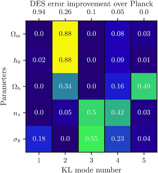
The fractional Fisher information on cosmological parameters for Planck computed using the KL modes from its update with simulated DES. Each line shows the fractional contribution of each KL mode to the total information on a given parameter. The sum of values in each row is one. The numbers on top of the figure show the fractional error improvement of DES over Planck for each KL mode.
We use the implementation of QUDM and related KL decomposition algorithms in the tensiometer code.
4.5 Goodness-of-fit loss
Notice that this estimator requires Gaussianity in both data space and parameter space. This is a stronger requirement than just approximate Gaussianity in parameter space, and limits its applicability in practice. Most of the likelihoods that we use here are Gaussian in data space with the exception of the large-scale CMB likelihood. This can be thought to be a prior on the optical depth of re-ionization, τ, which would not contribute to the tension budget since it is not shared with DES and hence allows us to use QDMAP.
We use the implementation of QDMAP in the tensiometer code.
4.6 Eigentension
The goal of the eigentension parameter-space method is to identify well-measured eigenmodes in the data and compare the parameter constraints of two experiments within the subspace spanned by the well-measured eigenmodes. Here, we briefly describe the steps taken to quantify the tension between the fiducial Planck and DES constraints in this paper, and refer the reader to Park & Rozo (2019) for a more detailed discussion and testing of the method.
We begin by identifying the well-measured parameter subspace by following these steps:
Obtain the parameter covariance matrix from a set of fiducial constraints for DES and identify the eigenvectors of this covariance matrix.
For each eigenvector, take the ratio of its variance in the prior to its variance in the posterior. If this ratio is above 102, identify the eigenvector as well-measured or robust.
Project the fiducial Planck constraints and the various DES constraints along the subspace spanned by the robust eigenvector(s), and create importance sampled chains of equal length for each constraint.
construct the chain of differences Δe = ei − ej between the importance sampled chains for i and j.
approximate the probability surface for Δe via KDE , and identify the iso-probability contour that crosses the origin, i.e. Δe = 0N, where N is the number of robust eigenvectors identified.
integrate the probability surface within the origin-crossing contour, and convert the integral to Gaussian sigmas.
For (ii), we use a Gaussian KDE with bandwidths determined from Silverman’s rule of thumb, and a straightforward Monte Carlo integration with 1.28 × 10⁷ random draws, which is sufficient to quantify tensions up to 5.4σ.
4.7 Other metrics
As mentioned in the introductions, a plethora of methods to quantify tension can be found in the cosmological literature. Our work does not investigate all of these methods, as this would make the analysis too wide in scope. For example, Hyperparameters (Hobson, Bridle & Lahav 2002; Luis Bernal & Peacock 2018) are more useful to construct a posterior from data sets in tension, by factoring in possible unknown systematic effects. The surprise (Seehars et al. 2016) is best suited for experiments that are an update from a previous version with less data. PPDs (Feeney et al. 2019) are similar in nature to the evidence ratio as shown in Lemos et al. (2020). Other methods are not considered as they closely resemble others, such as Amendola et al. (2013), Martin et al. (2014), and Joudaki et al. (2017) being based on the Bayesian Evidence ratio, and Lin & Ishak (2017a), Adhikari & Huterer (2019), and Lin & Ishak (2019) being different versions of parameter differences in update form.
5 RESULTS USING SIMULATED DES DATA
In this section, we apply the tension metrics described in Section 4 to the simulated vectors obtained as outlined in Section 3, and compare the results to our a priori expectation from Section 3. Our results are shown in Table 3 and graphically illustrated in Fig. 6.
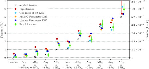
A graphical illustration of the main results of Table 3. Different points show the tension calculated by each tension metric as a function of the input shifts. The error bars in the green points correspond to sampling errors, which can be calculated for evidence-based methods by re-sampling the nested sampling weights.
We first note that our estimates of a priori Gaussian tension should be only used as an rough indication and are generally lower than the tension evaluated by the metrics that we study. This is because the a priori Gaussian tension does not have noise in the data vector while the tensions simulations do. This noise realization is the same for all the shifts, which explains the fact that the a priori tension is systematically lower in all results with respect to other tension estimators. We can see this in the baseline case, where in a noiseless case all metrics would obtain perfect agreement (a ‘0σ’ tension), but instead the noise leads to small discrepancies.
When applying parameter-shift estimators in both MCMC and update form we can see, from Table 3 and Fig. 6, that, for tensions measured up to 5σ, the two estimates agree very well, to within 0.3σ. This overall result is reassuring since these two estimators are measuring the same sense of tension between the two data sets. This agreement is also expected since the distributions that we consider are roughly Gaussian in the bulk of the distribution. At high statistical significance, MCMC results are lower in both cases and this suggests that the decay of the tails of the distribution is slower than a Gaussian distribution. For the parameter update, we observe that the two parameter combinations, discussed in Section 4.4, DES+Planck significantly improves over Planck-only do not appreciably change throughout the test cases.
In case of either fully informative or uninformative priors, the statistical significance of Goodness of Fit (GoF) loss is expected to match the one reported by parameter-shift estimators. As we can see from Table 3 that is the case at low statistical significance. Non-Gaussianities in the form of slowly decaying tails violate the assumptions used by the GoF loss estimator, while their impact can be mitigated by parameter shifts in update form. As a result, as statistical significance increases, in Table 3 the two estimates differ. In particular, as expected, GoF loss overestimates statistical significance since this estimator is assuming Gaussian decay in the tails.
For eigentension, we make use of the metric on the simulated vectors, making use of the robust DES eigenvector and the Monte Carlo sampling procedure discussed in Section 4.6. Note that the eigentension metrics are calculated only up to 5.4σ, or 1 in 1.28 × 10⁷; beyond this probability we simply quote that the tension is greater than 5.4σ and consider the tension to be definitive. The results are in good agreement with other tension metrics, in particular the two parameter shift estimators, with which eigentension shares the general approach of quantifying tensions at the parameter space level.
With suspiciousness, as shown in Table 3 and in Fig. 6, we obtain good agreement with the rest of tension metrics, especially when we consider the sampling error estimated from repeated re-samplings for the weights of the chain. To assign a tension probability, we need to calculate the Bayesian Model Dimensionality, for which we get d = 2.3 ± 0.1. At high statistical significance, suspiciousness seems to agree particularly well with GoF loss. This is reassuring since the two estimators coincide in the Gaussian limit with uninformative priors.
In Table 3, we also show the results for the Bayes ratio, interpreted with the Jeffreys’ scale as used by Abbott et al. (2018), and shown in Table 2. As we can see from the table, the interpretation of R transitions very quickly from ‘Strong Agreement’ to ‘Strong Tension’. To further investigate the relation between R and the other metrics, we plot them against each other in Fig. 7. This immediately highlights that the Jeffreys’ scale that we use to interpret the Bayes ratio results lacks granularity in how it quantifies physical tensions. Coherently across different estimators the interpretation of R goes from one extreme case to the other in a probability interval that covers about one standard deviation. Fig. 7 also clearly shows the bias of the evidence ratio toward agreement. The value of R = 1, which separates agreement and disagreement for our choice of priors is at a probability level that roughly corresponds to 3σ (i.e. a probability of the discrepancy occurring by chance of pT ∼ 0.003). We note that the offset between R = 1 and |$50{{\ \rm per\ cent}}$| probability events is set by the prior width and would hence change when changing the prior. Fig. 7 also shows that the evidence ratio, interpreted with the Jeffreys’ scale, would still signal a strong tension, if present, while lacking granularity in the discrimination of mildly statistically significant tensions.
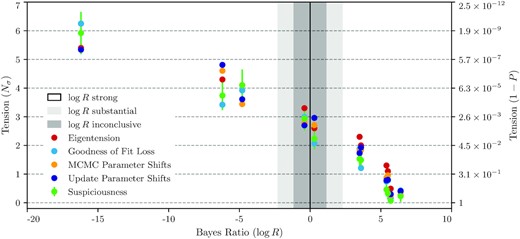
Tension estimates given by different metrics versus the corresponding Bayes ratio. Shaded regions highlight Jeffreys’ scale used to interpret the Bayes ratio, with the vertical line separating ‘Tension’ to the left and ‘Agreement’ to the right.
| log R | Interpretation |
|---|---|
| >2.3 | Strong agreement |
| (1.2,2.3) | Substantial agreement |
| (− 1.2, 1.2) | Inconclusive |
| (− 2.3, −1.2) | Substantial tension |
| <−2.3 | Strong tension |
| log R | Interpretation |
|---|---|
| >2.3 | Strong agreement |
| (1.2,2.3) | Substantial agreement |
| (− 1.2, 1.2) | Inconclusive |
| (− 2.3, −1.2) | Substantial tension |
| <−2.3 | Strong tension |
| log R | Interpretation |
|---|---|
| >2.3 | Strong agreement |
| (1.2,2.3) | Substantial agreement |
| (− 1.2, 1.2) | Inconclusive |
| (− 2.3, −1.2) | Substantial tension |
| <−2.3 | Strong tension |
| log R | Interpretation |
|---|---|
| >2.3 | Strong agreement |
| (1.2,2.3) | Substantial agreement |
| (− 1.2, 1.2) | Inconclusive |
| (− 2.3, −1.2) | Substantial tension |
| <−2.3 | Strong tension |
In Section 4, we made a distinction between parameter-space methods and evidence-based methods. We find that all our tension metrics agree well not only amongst themselves, but also qualitatively with the a priori Gaussian tension calculations described in Section 3. This is a non-trivial result, as both the calculations and the fundamental questions that the various methods are trying to address differ.
The only exceptions to this good agreement are given by the statistically significant σ8 shifts where the spread between the three parameter difference estimators is smaller than the difference between them GoF loss and suspiciousness; and the smaller a priori shifts in Ωm, for which the a priori Gaussian tension estimate is smaller than the results from eigentension and suspiciousness. Since the input calculation used a noiseless data vector and simulated DES data vectors had noise, these disagreements are expected. They are likely to be caused by the noise introduced in the chains used by the tension metrics, and will have a more significant impact on the small shifts.
Based on these results, we propose a methodology to quantify tension between data sets that exploits the strengths of all the different methods, summarized by Fig. 8. Within the parameter-based approach, we recommend to generate a Monte Carlo parameter difference distribution and observe where the zero-difference point stands provided we have enough samples of the posterior distribution in its tail, as this method has no problem with non-Gaussianities, and has the advantage of providing useful visualizations in the form of confidence regions generated directly from the difference chain itself. However, if the number of samples in the tension tail is insufficient, this parameter-difference distribution will not be reliable enough to make statements about tension. In this case, either Eigentension or parameter differences in update form provide reliable metrics of tension. These two methods are also useful in identifying the physics behind the tension, as they provide characteristic parameter combinations along with the identified tensions lie. Since it does not offer mitigation of non-Gaussianities, we do not recommend using goodness-of-fit loss on its own, but rather as a cross-check with other metrics.
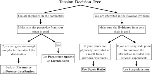
A practical ‘decision tree’ to measure tension, illustrating when each tension metric should be used.
For the evidence-based methods, if we have a well-motivated prior, such as the posterior from a previous experiment or a physically motivated one, we can calculate the tension using the Bayes ratio. However, as discussed in the text, experiments such as DES and Planck often choose wide priors in order to obtain posteriors that do not depend on previous experiments. The arbitrariness in the choice of width of those priors means that we cannot use the Bayes ratio, as discussed in Section 4.1, unless we calibrated R using Fig. 7, but that would require recalibration if any details of the analysis changed. In the case of wide and uninformative priors, the suspiciousness answers the same question as the Bayes ratio but correcting for the prior volume effect. We recommend its use over the Bayes ratio in general since it has the additional desirable property of having a ‘tension probability’ interpretation under a Gaussian approximation, without any need for calibration.
As pointed out in Fig. 8, different methods require reliable calculations of different quantities. Parameter-space methods require a good estimate of the posterior, and particularly of its mean and covariance matrix. Evidence-based methods require a calculation of the Bayesian evidence. Therefore, our choice of tension metric should inform our sampling choices, as further discussed in The Dark Energy Survey Collaboration (2020).
6 APPLICATION TO DES Y1 AND PLANCK
With a better understanding of the interpretation of each of the tension metrics, we now revisit the issue of consistency between the DES Y1 cosmology results and those obtained by the Planck collaboration (Planck Collaboration 2016, 2018). This also serves as a worked example on real data of how tension between experiments can be fully quantified.
We choose to investigate three different combinations of DES data sets: (1) weak lensing-only constraints from Troxel et al. (2018); (2) constraints from combining the auto and cross-correlation between weak lensing and galaxy clustering, referred to as the 3 × 2pt analysis; and (3) constraints from (2) plus cross-correlation with CMB lensing, referred as the 5 × 2pt analysis (Abbott et al. 2019). We particularly focus in the second combination, as it provided the most powerful constraints from large-scale structure measured by DES alone. For Planck 2015, we use the small-scale (ℓ > 30) measurements of the CMB temperature power spectrum and the joint large-scale temperature and polarization data. For Planck 2018, we use small-scale CMB temperature, polarization, and their cross-correlation measurements combined with large-scale temperature and and E-mode polarization data. In doing so, we follow the recommendations of the Planck collaboration in the two data releases.
The results of parameter estimation for these data sets are shown in Fig. 9 and the results of different tension estimators in Table 4. We highlight in the table the results that we focus our discussion on.9
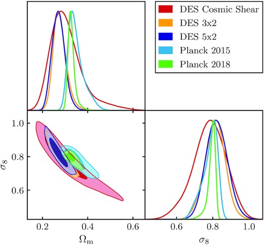
|$68 {{\ \rm per\ cent}}$| and |$95 {{\ \rm per\ cent}}$| confidence regions of the joint marginalized posterior probability distributions for DES Year 1 Cosmic Shear, 3 × 2pt and 5 × 2pt likelihoods, and for the Planck 2015 TTTEEE likelihood.
We start with MCMC parameter shifts, as it is the parameter-based method that can give the most accurate value for the tension, thanks to its ability to go beyond the Gaussian approximation. In Fig. 10, we can see the posterior of differences between the determination of σ8 and Ωm from different DES data sets and Planck that clearly shows a tension that is greater than 2σ. In Table 4, we see that in full parameter space this tension is at the 2.2σ level. We proceed with suspiciousness as our recommended evidence-based method which fully confirms the parameter-shift results, giving a 2.4 ± 0.2σ tension between Planck 2015 and DES 3 × 2pt. We note that applying both methods provides a useful cross-check of their respective results. This moderate tension remains when Planck is updated from the 2015 to the 2018 data and for DES 5 × 2pt. This shows that this tension is robust to the inclusion of CMB polarization data.
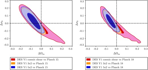
Joint marginalized posterior distribution of the parameter differences between different DES data selections and Planck 15/18. The distribution of parameter differences is used to compute the statistical significance of a parameter shift. The darker and lighter shading corresponds to the |$68{{\ \rm per\ cent}}$| and |$95{{\ \rm per\ cent}}$| C.L. regions, respectively.
To understand the physics behind these discrepancies, it is useful to consider other methods. Using eigentension, we identify a single well-measured eigenmode for each DES analysis: |$\sigma _8 \Omega _\mathrm{m}^{0.57}$| for the 3 × 2pt analysis, and |$\sigma _8 \Omega _\mathrm{m}^{0.58}$| in the 5 × 2pt case. Both eigenmodes are very similar to the widely used definition of S8 = σ8(Ωm/0.3)0.5, and can be interpreted as representing the ‘lensing strength’ arising from the large-scale structure of the late-time universe. After measuring tension exclusively along this direction in parameter space, we find results that are in agreement with other methods. This shows that the moderate tension between DES and Planck is found along a parameter space direction that we believe DES is robustly measuring. Studying parameter updates of DES with respect to Planck gives similar conclusions. As discussed in the previous section and shown in Fig. 5, combining DES improves the Planck determination of two parameters, the first mode projecting mostly on to σ8 and the second on to Ωmh2. The first mode drives most of the tension while the shift in the second is compatible with a statistical fluctuation. Decrease in goodness of fit agrees with other estimators.
The Bayes ratio interpreted on the Jeffreys’ scale reports no significant tension between all data combinations that we consider. Given the results of the previous section, we can understand this as the data tension not overcoming the bias of the Bayes ratio towards agreement. We note that the priors used for the fiducial analyses in the previous section do not coincide with the priors used in this section; we thus cannot use the previously derived calibration of the Bayes ratio.
The mild tension we obtain between Planck and DES, varying between 2σ and 3σ, should not be overlooked. While this level of tension could still be a statistical fluke, it is significant enough to warrant in-depth future investigations. The forthcoming DES Y3 analysis, incorporating a larger fraction of the sky, is expected to shed light on this matter.
7 CONCLUSIONS
In this work, we have explored different methods to quantify consistency between two uncorrelated data sets, focusing on the comparison between DES and Planck. The motivation is to decide on a metric of tension between these two surveys ahead of the DES Y3 data release. This was done by simulating a set of DES data sets with values of cosmological parameters chosen to introduce varying levels of discrepancy with Planck. We calculate the tension for each simulated DES data set, and compare to an a priori Gaussian tension expected based on the known true cosmologies for the simulated data sets. While this work has been performed for the specific case of DES and Planck, our findings about the different metrics described in Section 5 apply to any problem of tension quantification. However, if we wanted to apply the Bayes ratio to a different problem with uninformative priors, the exercise of calibrating the Bayes ratio would have to be repeated.
We have found that the Bayes’ ratio used in the Y1 analysis has several flaws that make it unsuitable for the quantitative comparison of DES and Planck. In particular, it is proportional to the width of the chosen uninformative prior; it relies on the Jeffreys’ scale to interpret the ratio of probabilities, which needs an unknown calibration that is problem-dependent (i.e. we would need to build a table such as Table 3 in every problem to calculate the overall calibration of the Bayes ratio); and the fact that we can only calculate logarithms of the probability ratio means that the Jeffreys’ scale used in the DES Y1 analysis (Table 2) will in most cases diagnose extreme agreement or extreme tension.
The tension between Planck and simulated DES chains for different shifts in σ8 and Ωm, calculated via the different tension metrics described in the main text. The first column refers to the number of 1D standard deviations by which each parameter is shifted, defined in equation (2). The a priori Gaussian tension is calculated as described in Section 3 and serves only as an order of magnitude approximation of expected results. The probability results of each of the tension metrics is converted to a number of effective sigmas using equation (4).
| 1D shift | a priori | Bayes ratio | Eigentension | GoF Loss | MCMC/Update | Suspiciousness | |
|---|---|---|---|---|---|---|---|
| Tension | log R | Interpretation | Param Diffs | ||||
| Baseline | |$0 \, \sigma$| | 5.7 ± 0.6 | Strong agreement | |$0.5\, \sigma$| | |$0.2\, \sigma$| | |$0.3/0.3\, \sigma$| | |$(0.1 \pm 0.1) \, \sigma$| |
| Δσ8 = −0.5 × δσ8 | |$0.0 \, \sigma$| | 6.4 ± 0.6 | Strong agreement | |$0.4\, \sigma$| | |$0.4\, \sigma$| | |$0.3/0.4\, \sigma$| | |$(0.2 \pm 0.2) \, \sigma$| |
| ΔΩm = 0.5 × δΩm | |$0.1 \, \sigma$| | 5.4 ± 0.6 | Strong agreement | |$1.3\, \sigma$| | |$0.7\, \sigma$| | |$0.9/0.8\, \sigma$| | |$(0.5 \pm 0.2) \, \sigma$| |
| Δσ8 = −1 × δσ8 | |$0.4 \, \sigma$| | 5.5 ± 0.6 | Strong agreement | |$1.1\, \sigma$| | |$0.8\, \sigma$| | |$1.0/0.8\, \sigma$| | |$(0.3 \pm 0.2) \, \sigma$| |
| ΔΩm = 1 × δΩm | |$1.0 \, \sigma$| | 3.5 ± 0.5 | Strong agreement | |$2.3\, \sigma$| | |$1.9\, \sigma$| | |$1.8/1.7\, \sigma$| | |$(1.5 \pm 0.3) \, \sigma$| |
| Δσ8 = −1.5 × δσ8 | |$1.1 \, \sigma$| | 3.6 ± 0.6 | Strong agreement | |$2.0\, \sigma$| | |$1.2\, \sigma$| | |$1.8/1.9\, \sigma$| | |$(1.5 \pm 0.3) \, \sigma$| |
| ΔΩm = 1.5 × δΩm | |$2.3 \, \sigma$| | −0.4 ± 0.6 | No evidence | |$3.3\, \sigma$| | |$3.0\, \sigma$| | |$2.8/2.7\, \sigma$| | |$(2.9 \pm 0.4) \, \sigma$| |
| Δσ8 = −2 × δσ8 | |$2.0 \, \sigma$| | 0.3 ± 0.6 | No evidence | |$2.6\, \sigma$| | |$2.1\, \sigma$| | |$2.7/3.0\, \sigma$| | |$(2.2 \pm 0.4) \, \sigma$| |
| ΔΩm = 2 × δΩm | |$3.8 \, \sigma$| | −4.8 ± 0.6 | Strong tension | |$4.1\, \sigma$| | |$3.9\, \sigma$| | |$3.4/3.6\, \sigma$| | |$(4.1 \pm 0.6) \, \sigma$| |
| Δσ8 = −3 × δσ8 | |$3.7 \, \sigma$| | −6.2 ± 0.6 | Strong tension | |$4.3\, \sigma$| | |$3.4\, \sigma$| | |$4.6/4.8\, \sigma$| | |$(3.7 \pm 0.5) \, \sigma$| |
| ΔΩm = 3 × δΩm | |$\gt 5 \, \sigma$| | −16.2 ± 0.6 | Strong tension | |$\gt 5.4\, \sigma$| | |$6.2\, \sigma$| | |$5.3/5.3\, \sigma$| | |$(5.9 \pm 0.7) \, \sigma$| |
| Δσ8 = −5 × δσ8 | |$\gt 5 \, \sigma$| | −26.3 ± 0.6 | Strong tension | |$\gt 5.4\, \sigma$| | |$5.8\, \sigma$| | |$6.8/8.8\, \sigma$| | |$(6.3 \pm 0.8) \, \sigma$| |
| ΔΩm = 5 × δΩm | |$\gt 5 \, \sigma$| | −47.0 ± 0.6 | Strong tension | |$\gt 5.4\, \sigma$| | |$10.0\, \sigma$| | |$6.6/8.1\, \sigma$| | |$(9.6 \pm 1.2) \, \sigma$| |
The tension between Planck and different data set combinations involving DES Y1 data, calculated via the different tension metrics described in the main text. In the first column, Planck refers to the combination of the TT, TE, and EE likelihoods. In bold font, we highlight the combinations of DES 3 × 2pt and Planck, as those are the main focus of this section. The horizontal line separates Planck 2015 and 2018 data set combinations.
| Data set | Bayes ratio | Eigentension | GoF Loss | MCMC/Update | Suspiciousness | |
|---|---|---|---|---|---|---|
| log R | Interpretation | Param Shifts | ||||
| DES cosmic shear versus Planck 15 | 2.2 ± 0.5 | Substantial agreement | |$1.8\, \sigma$| | |$1.3 \, \sigma$| | |$1.3/1.2 \, \sigma$| | |$(0.7 \pm 0.4) \, \sigma$| |
| DES 3 × 2pt versusPlanck15 | 1.0 ± 0.5 | No evidence | |$2.4\, \sigma$| | |$2.7\, \sigma$| | |$2.2/2.2 \, \sigma$| | |$(2.4 \pm 0.2) \, \sigma$| |
| DES 5 × 2pt versus Planck 15 | 1.1 ± 0.5 | Substantial agreement | |$2.4\, \sigma$| | |$2.8\, \sigma$| | |$2.1/2.3 \, \sigma$| | |$(2.2 \pm 0.3) \, \sigma$| |
| DES 5 × 2pt versus Planck 15 + lensing | 1.0 ± 0.6 | No evidence | |$2.4\, \sigma$| | |$2.5\, \sigma$| | |$2.1/2.3 \, \sigma$| | |$(2.2 \pm 0.4) \, \sigma$| |
| DES 5 × 2pt + Planck lensing versus Planck 15 | 6.1 ± 0.6 | Strong agreement | |$1.6\, \sigma$| | |$2.4\, \sigma$| | |$1.9/2.2 \, \sigma$| | |$(1.8 \pm 0.2) \, \sigma$| |
| DES cosmic shear versus Planck 18 | 3.3 ± 0.4 | Strong agreement | |$1.5\, \sigma$| | |$1.0\, \sigma$| | |$1.0/1.1 \, \sigma$| | |$(0.5 \pm 0.3) \, \sigma$| |
| DES 3 × 2pt versusPlanck18 | 2.2 ± 0.6 | Substantial agreement | |$2.2\, \sigma$| | |$1.6\, \sigma$| | |$2.0/2.3 \, \sigma$| | |$(2.4 \pm 0.2) \, \sigma$| |
As shown in Table 3, the other four tension metrics employed in this work – eigentension, GoF loss, parameter differences, and suspiciousness – agree with the a priori tension, as well as amongst themselves, with the exceptions of small shifts in Ωm and large shifts in σ8 discussed in Section 5, which are likely the result of noise introduced in the simulated data vectors. We conclude that any of the tension metrics can be used for the problem of quantifying tension between DES and Planck, as they produce similar results.
We use these tension metrics to re-assess the tension between DES Y1 and Planck 2015, as well as with the latest Planck 2018 results. We find, similar to our findings from the simulated analyses that the dependence of the evidence ratio on calibration causes the results to be inconsistent with what we see in the plots, and what all other tension metrics indicate. We find that there is a ∼2.3σ between DES and Planck, which remains when the Planck 2018 likelihood is used. It remains to be seen how this will evolve when the more powerful DES Y3 data are used. If the tension is reduced when more data are considered, we are likely looking at a statistical fluctuation. If the tension remains or increases, we could be looking at unexplained systematics in either of the surveys, or evidence of physics beyond the ΛCDM model.
ACKNOWLEDGEMENTS
Funding for the DES Projects has been provided by the U.S. Department of Energy, the U.S. National Science Foundation, the Ministry of Science and Education of Spain, the Science and Technology Facilities Council of the United Kingdom, the Higher Education Funding Council for England, the National Center for Supercomputing Applications at the University of Illinois at Urbana-Champaign, the Kavli Institute of Cosmological Physics at the University of Chicago, the Center for Cosmology and Astro-Particle Physics at the Ohio State University, the Mitchell Institute for Fundamental Physics and Astronomy at Texas A&M University, Financiadora de Estudos e Projetos, Fundação Carlos Chagas Filho de Amparo à Pesquisa do Estado do Rio de Janeiro, Conselho Nacional de Desenvolvimento Científico e Tecnológico and the Ministério da Ciência, Tecnologia e Inovação, the Deutsche Forschungsgemeinschaft and the Collaborating Institutions in the Dark Energy Survey.
The Collaborating Institutions are Argonne National Laboratory, the University of California at Santa Cruz, the University of Cambridge, Centro de Investigaciones Energéticas, Medioambientales y Tecnológicas-Madrid, the University of Chicago, University College London, the DES-Brazil Consortium, the University of Edinburgh, the Eidgenössische Technische Hochschule (ETH) Zürich, Fermi National Accelerator Laboratory, the University of Illinois at Urbana-Champaign, the Institut de Ciències de l’Espai (IEEC/CSIC), the Institut de Física d’Altes Energies, Lawrence Berkeley National Laboratory, the Ludwig-Maximilians Universität München and the associated Excellence Cluster Universe, the University of Michigan, NFS’s NOIRLab, the University of Nottingham, The Ohio State University, the University of Pennsylvania, the University of Portsmouth, SLAC National Accelerator Laboratory, Stanford University, the University of Sussex, Texas A&M University, and the OzDES Membership Consortium.
Based, in part, on observations at Cerro Tololo Inter-American Observatory at NSF’s NOIRLab (NOIRLab Prop. ID 2012B-0001; PI: J. Frieman) which is managed by the Association of Universities for Research in Astronomy (AURA) under a cooperative agreement with the National Science Foundation.
The DES data management system is supported by the National Science Foundation under grant numbers AST-1138766 and AST-1536171. The DES participants from Spanish institutions are partially supported by Ministerio de Ciencia e Innovación (MICINN) under grants ESP2017-89838, PGC2018-094773, PGC2018-102021, SEV-2016-0588, SEV-2016-0597, and MDM-2015-0509, some of which include ERDF funds from the European Union. IFAE is partially funded by the Centres de Recerca de Catalunya (CERCA) program of the Generalitat de Catalunya. Research leading to these results has received funding from the European Research Council under the European Union’s Seventh Framework Program (FP7/2007-2013) including ERC grant agreements 240672, 291329, and 306478. We acknowledge support from the Brazilian Instituto Nacional de Ciência e Tecnologia (INCT) do e-Universo (CNPq grant 465376/2014-2).
This manuscript has been authored by Fermi Research Alliance, LLC under Contract No. DE-AC02-07CH11359 with the U.S. Department of Energy, Office of Science, Office of High Energy Physics.
PL acknowledges the Science and Technology Facilities Council (STFC) Consolidated grants ST/R000476/1 and ST/T000473/1. We also thank the organizers of the DES Y3 workshop: “Probing Dark Energy Observations in the Nonlinear Regime” at the University of Michigan in Ann Arbor, where this project started.
DATA AVAILABILITY STATEMENT
The data underlying this article are available in the Dark Energy Survey Data Management platform, at https://des.ncsa.illinois.edu
Footnotes
Here, σ8 is the present-day linear theory root-mean-square amplitude of the matter fluctuations averaged in spheres of radius 8 h−1 Mpc.
In this paper, the terms ‘marginalized over’ and ‘projected’ both mean ‘integrated over the other parameters’.
As pointed out by Handley & Lemos (2019), non-Gaussian posteriors can be ‘Gaussianized’ using Box–Cox transformations (Box & Cox 1964; Joachimi & Taylor 2011; Schuhmann, Joachimi & Peiris 2016) that preserve the value of S. Therefore, the chi-squared interpretation of S derived in the Gaussian case can be approximately valid even for posteriors that do not look Gaussian, even if it is not guaranteed that both posteriors can be Gaussianized simultaneously.
In the case of weighted samples, the weight of the parameter difference sample is the product of the two weights.
The reader might notice that the values of the Bayes ratio reported in Table 4, in particular for the case DES 3 × 2pt versus Planck 15, differ from the values reported by Abbott et al. (2018; R = 6.6). This difference has been identified as originating from sampling issues in the DES Y1 analysis, as will be described in more detail in The Dark Energy Survey Collaboration (2020).
REFERENCES
APPENDIX A: DARK ENERGY SURVEY DATA
The DES (The Dark Energy Survey Collaboration 2005; Abbott et al. 2016) is a 6-yr survey that has observed over 5000 deg2 in five filters (grizY) and has probed redshifts up to z ∼1.3. It has also used time-domain to measure several thousand type Ia supernovae (SNe Ia). DES can constrain cosmological parameters in several ways: It can use these SNe Ia, and treat them as standarizable candles to constrain cosmology through their redshift–luminosity relation, usually referred to as Hubble Diagram (Hubble 1929; Kirshner 2004); it can use the distribution of galaxies to measure the Baryon Acoustic Oscillation (BAO) feature which was imprinted by sound waves at the recombination era (z ∼1100), and which serves as a standard ruler (Eisenstein, Seo & White 2007); it can use the abundance of galaxy clusters, the largest gravitationally bound structures in the Universe (Allen, Evrard & Mantz 2011); it can use the distribution of galaxies to measure the dark matter density distribution, under the assumption of some bias relating the two, called galaxy clustering; and it can measure the distortion of light by intervening matter along the line of sight, referred to as gravitational lensing (Mandelbaum 2018). When the matter distribution distorting the path of light is the large-scale structure of the Universe, the effect is called cosmic shear (Kilbinger 2015). Because in this case distortions are too small to be detected for individual galaxies, they are detected through correlations in the shapes and position of galaxies images.
Using data from the first year of observations (Y1), the DES collaboration has already reported constraints on cosmology from BAO (The Dark Energy Survey Collaboration 2017), galaxy clustering (Elvin-Poole et al. 2018), cosmic shear (Troxel et al. 2018), the cross-correlation of galaxy clustering and cosmic shear, referred to as galaxy–galaxy lensing (Prat et al. 2018), and as a main result, the combination of the two-point functions from cosmic shear, galaxy clustering, and galaxy–galaxy lensing, henceforth referred to as ‘3 × 2pt’ (Abbott et al. 2018). In addition, using data from 3 yr of observations (Y3), DES has also constrained cosmology from SNe Ia (Abbott et al. 2019a), and galaxy clusters (To et al. 2020). However, as described in Abbott et al. (2019b), the most powerful constraints from future DES data releases will come from combinations of the different probes, as these can break degeneracies in parameter constraints and significantly increase accuracy.
We adopt the same priors used in the DES Y1 analysis, shown in Table A1.
Cosmological and nuisance parameters and their priors used in this analysis.
| Parameter | Prior |
|---|---|
| Cosmology | |
| Ωm | flat (0.1, 0.9) |
| As | flat (5 × 10⁻¹⁰, 5 × 10⁻⁹) |
| ns | flat (0.87, 1.07) |
| Ωb | flat (0.03, 0.07) |
| h | flat (0.55, 0.90) |
| Ωνh2 | flat(5 × 10⁻⁴, 10−2) |
| Lens galaxy bias | |
| bi(i = 1, 5) | flat (0.8, 3.0) |
| Intrinsic alignment | |
| AIA | flat (−5, 5) |
| ηIA | flat (−5, 5) |
| Lens photo-z shift (red sequence) | |
| |$\Delta z^1_{\rm l}$| | Gauss (0.0, 0.007) |
| |$\Delta z^2_{\rm l}$| | Gauss (0.0, 0.007) |
| |$\Delta z^3_{\rm l}$| | Gauss (0.0, 0.006) |
| |$\Delta z^4_{\rm l}$| | Gauss (0.0, 0.01) |
| |$\Delta z^5_{\rm l}$| | Gauss (0.0, 0.01) |
| Source photo-z shift | |
| |$\Delta z^1_{\rm s}$| | Gauss (0.0, 0.016) |
| |$\Delta z^2_{\rm s}$| | Gauss (0.0, 0.013) |
| |$\Delta z^3_{\rm s}$| | Gauss (0.0, 0.011) |
| |$\Delta z^4_{\rm s}$| | Gauss (0.0, 0.022) |
| Shear calibration | |
| mi(i = 1, 4) | Gauss (0.0, 0.023) |
