


ABSTRACT
The amount of mass lost by stars during the red-giant branch (RGB) phase is one of the main parameters to understand and correctly model the late stages of stellar evolution. Nevertheless, a fully comprehensive knowledge of the RGB mass-loss is still missing. Galactic Globular Clusters (GCs) are ideal targets to derive empirical formulations of mass-loss, but the presence of multiple populations with different chemical compositions has been a major challenge to constrain stellar masses and RGB mass-losses. Recent work has disentangled the distinct stellar populations along the RGB and the horizontal branch (HB) of 46 GCs, thus providing the possibility to estimate the RGB mass-loss of each stellar population. The mass-losses inferred for the stellar populations with pristine chemical composition (called first-generation or 1G stars) tightly correlate with cluster metallicity. This finding allows us to derive an empirical RGB mass-loss law for 1G stars. In this paper, we investigate seven GCs with no evidence of multiple populations and derive the RGB mass-loss by means of high-precision Hubble-Space Telescope photometry and accurate synthetic photometry. We find a cluster-to-cluster variation in the mass-loss ranging from ∼0.1 to ∼0.3 M⊙. The RGB mass-loss of simple-population GCs correlates with the metallicity of the host cluster. The discovery that simple-population GCs and 1G stars of multiple population GCs follow similar mass-loss versus metallicity relations suggests that the resulting mass-loss law is a standard outcome of stellar evolution.
1 INTRODUCTION
A proper understanding of the late stages of stellar evolution depends on the precise knowledge of the law ruling mass-loss along the red giant branch (RGB). Hence, determining the RGB mass-loss law is a crucial step to fully understand stellar evolution.
To date, we still lack a conclusive theoretical description of RGB mass-loss, and we mostly rely on empirical determinations. Historically, the law by Reimers (1975) based on Population I stars has represented for decades the state of the art for describing RGB mass-loss (see also Fusi-Pecci & Renzini 1978; Catelan 2000, and references therein). More recently, new formulations, based on magnetohydrodynamics, have been proposed (see Schröder & Cuntz 2005, 2007; Cranmer & Saar 2011) either as new law or as modifications of the Reimers (1975) one. These new formulations tie mass-loss to the interactions between surface turbulence and the magnetic field of the stars which are most relevant in the last part of the RGB where, indeed, most of the mass-loss is predicted to take place.
A constantly updated observational framework is therefore crucial in the calibration and construction of the theoretical framework. Origlia et al. (2007, 2014) estimated the mass-loss of 47 Tucanae and other 14 GCs based on the excess of mid-infrared (IR) light and suggested that a fraction of stars can lose mass at any RGB luminosity. To do this, they exploited multiband photometry from the Spitzer space telescope and from near-infrared (NIR) ground-based facilities (but see Boyer et al. 2010; McDonald et al. 2011a, for a different interpretation of the photometric results by Origlia and collaborators). Momany et al. (2012) on the other hand did not detect any NIR excess among RGB stars of 47 Tucanae. Mass-loss has been also estimated by using Spitzer Infrared Spectrograph spectra of RGB stars, a technique adopted by McDonald, Johnson & Zijlstra (2011b) to investigate the brightest RGB stars in ω Centauri.
The comparison between the stellar mass of horizontal branch (HB) and RGB stars may provide an efficient approach to infer the RGB mass-loss in a simple stellar population. Indeed, after reaching their tip luminosity, RGB stars undergo the so-called helium flash, namely an abrupt ignition of their degenerate helium core. After this violent process, HB stars reach their position along the branch with different effective temperatures. The total mass deficit of the resulting stars with respect to the RGB progenitors represents the sought-after mass-loss. Based on this idea, Gratton et al. (2010) estimated the RGB mass-loss of 98 Galactic GCs, but the presence of multiple stellar populations with different chemical composition provides a significant challenge to their conclusions.
Indeed, in addition to mass-loss, the colour and the magnitude of a star along the HB depend on its age, metallicity, and helium content. While the majority of GCs hosts stars with the same age and metallicity, the majority of them are composed of two or more stellar populations with different helium content (e.g. D’Antona et al. 2002, 2005; Lagioia et al. 2018; Milone et al. 2018). As a consequence, different parameters with degenerate effects determine the effective temperature of an HB star. In particular, increased helium and RGB mass-loss would both increase the star temperature.
Recent work has introduced an innovative approach to infer the mass-loss of the distinct stellar populations in GCs (Tailo et al. 2019a, b). These papers are based on the theoretical and empirical evidence that stellar populations with different helium content populate distinct HB regions (e.g. D’Antona et al. 2002; Gratton et al. 2011; Marino et al. 2011, 2014; Dondoglio et al. 2020). Once stellar populations are identified along the HB and their helium content is independently constrained from the MS and RGB (Milone et al. 2018), it is possible to disentangle the effect of helium and mass-loss along the HB.
Tailo et al. (2020, hereafter T20) has extended this method to a large sample of 46 GCs. They identified their stellar population with pristine helium abundance (hereafter first-generation or 1G) along the RGB and the HB and inferred the RGB mass-loss by using appropriate theoretical models. Similarly, they estimated the mass-loss of stars with extreme helium content (hereafter extreme second generation or 2Ge). Tailo and collaborators found that the mass-loss of 1G stars changes from one cluster to another and is tightly correlated with the cluster metallicity. Based on these results they defined an empirical mass-loss law for 1G stars.
In this work, we analyse seven clusters with no evidence of multiple populations, namely NGC 6426, Palomar 12, Palomar 15, Pyxis, Ruprecht 106, Terzan 7, and Terzan 8. Hence, they are either simple stellar populations or host stars with very small internal helium variations. We compare the RGB mass-losses inferred from these clusters and from 1G and 2Ge stars of the multiple-population clusters studied by T20. The main goal is to shed light on whether the mass-loss law by T20 describes 1G stars of multiple-population GC alone or is a universal property of stellar evolution.
The paper is organized as follows: in Section 2, we present the photometric catalogues and the stellar evolution models. In Section 3, we describe the method to infer mass-loss and provide the results for all clusters, in Section 5. Finally, we compare the results from this paper and from T20 and summarize the main findings of the paper in Section 6.
2 DATA, DATA REDUCTION, AND SIMULATED PHOTOMETRY
The clusters studied in this paper are seven Galactic GCs older than ∼9 Gyr, whose HB stars exhibit short colour extensions as expected from simple populations. The sample includes Ruprecht 106, which is considered the prototype of simple-population clusters as neither high-resolution spectroscopy nor multiband photometry show evidence of internal variations in chemical composition (Villanova et al. 2012; Dotter et al. 2018; Lagioia et al. 2019). Pyxis and Palomar 12 are candidate simple-population clusters because their HB span a short colour range (Milone et al. 2014). Terzan 7 is considered a simple-population GC based on the spectroscopic analysis by Sbordone et al. (2005). In the case of Terzan 8 high-resolution spectroscopy has revealed that 19 out of 20 analysed stars are consistent with 1G stars (Carretta et al. 2014). These five clusters have all initial masses (Baumgardt & Hilker 2018; Baumgardt et al. 2019) smaller that ∼2 × 10⁵ M⊙, which is considered the mass threshold to form multiple populations in GCs (Milone et al. 2020). In this work, we consider these clusters as SSP GC candidates. We included in the sample Palomar 15 and NGC 6426, whose HBs have short colour extension but are more massive than ∼2 × 10⁵ M⊙. Despite there is no evidence that these two clusters have homogeneous chemical composition, the small colour extensions of their HBs suggest that their 2G stars, if present, would not exhibit extreme chemical compositions.
In addition, we analysed the CMDs of the candidate simple-population GCs AM 4, E 3, Palomar 1, and Palomar 13 (Monaco et al. 2018; Milone et al. 2020). By using literature photometric catalogues (Sarajedini et al. 2007; Anderson et al. 2008; Dotter, Sarajedini & Anderson 2011; Milone et al. 2016), we verified that no HB stars are present in these last four clusters. Nevertheless, we used their photometry to derive other quantities that are relevant for our analysis, including cluster age and the stellar mass at the tip of the RGB.
In the following, we summarize the photometric data-set and the stellar models that we employ to derive the RGB mass-loss in the seven clusters with HB stars.
2.1 Photometric data set
To infer the RGB mass-loss, we derived stellar photometry and proper motions by using two-epoch images collected through the F606W and F814W filters of the Wide Field Channel of the Advanced Camera for Surveys (WFC/ACS) on board HST. The main properties of the images are provided in Table 1.
Description of the HST images used in the paper.
| ID | Filter | date | N × Exptime | Program | PI |
|---|---|---|---|---|---|
| NGC 6426 | F606W | Aug 04 2009 | 45s+4 × 500s | 11586 | A. Dotter |
| NGC 6426 | F814W | Aug 04 2009 | 50s+4 × 540s | 11586 | A. Dotter |
| NGC 6426 | F606W | Aug 09 2016 | 50s+3 × 780s+3 × 781s | 14235 | S. Sohn |
| Palomar 12 | F606W | May 21 2006 | 60s+5 × 340s | 10775 | A. Sarajedini |
| Palomar 12 | F814W | May 21 2006 | 50s+5 × 340s | 10775 | A. Sarajedini |
| Palomar 12 | F606W | Jun 11 2016 | 65s+2 × 544s+2 × 545s+548s+3 × 549s | 14235 | S. Sohn |
| Palomar 15 | F606W | Oct 16 2009 | 10s+65s+8 × 550s | 11586 | A. Dotter |
| Palomar 15 | F814W | Oct 16 2009 | 10s+25s+55s+4 × 500s+4 × 525s+4 × 560s | 11586 | A. Dotter |
| Palomar 15 | F606W | Oct 09 2015 | 555s | 14235 | S. Sohn |
| Palomar 15 | F814W | Oct 09 2015 | 545s+3 × 546s+3 × 555s | 14235 | S. Sohn |
| Pixys | F606W | Oct 11 2009 | 50s+4 × 517s | 11586 | A. Dotter |
| Pixys | F814W | Oct 11 2009 | 55s+4 × 547s | 11586 | A. Dotter |
| Pixys | F606W | Oct 09 2015 | 50s+3 × 799s+3 × 800s | 14235 | S. Sohn |
| Ruprecht 106 | F606W | Jul 04 2010 | 55s+4 × 550s | 11586 | A. Dotter |
| Ruprecht 106 | F814W | Jul 10 2010 | 60s+3 × 585s+586s | 11586 | A. Dotter |
| Ruprecht 106 | F606W | Jul 12 2016 | 60s+841s+2 × 842s+845 + 2 × 845s | 14235 | S. Sohn |
| Terzan 7 | F606W | Jun 03 2006 | 40s+5 × 345s | 10775 | A. Sarajedini |
| Terzan 7 | F814W | Jun 03 2006 | 40s+5 × 345s | 10775 | A. Sarajedini |
| Terzan 7 | F606W | May 04 2016 | 45s+2 × 554s+2 × 555s+4 × 556s | 14235 | S. Sohn |
| Terzan 8 | F606W | Jun 03 2006 | 40s+5 × 345s | 10775 | A. Sarajedini |
| Terzan 8 | F814W | Jun 03 2006 | 40s+5 × 345s | 10775 | A. Sarajedini |
| Terzan 8 | F606W | Apr 28 2016 | 45s+2 × 554s+2 × 555s+4 × 556s | 14235 | S. Sohn |
Stellar magnitudes and positions have been derived for each exposure separately by using the img2xym|$\_$|WFC computer program from Anderson & King (2006). In a nutshell, we identified as a candidate star every point-like source whose central pixel has more than 50 counts within its 3 × 3 pixels and with no brighter pixels within a radius of 0.2 arcsec. The fluxes and positions of all candidate stars have been measured in each exposure by fitting the appropriate effective-PSF model. The stellar magnitudes of all exposures collected through the same filter are then averaged together to provide the best estimates of the instrumental F606W and F814W magnitudes. Instrumental magnitudes are then calibrated to the Vega system by using the photometric zero-points provided by the Space Telescope Science Institute website.1
Stellar position has been corrected for geometrical distortion by using the solution by Anderson & King (2006) and transformed into a common reference frame based on Gaia early data release 3 (Gaia EDR3; Gaia Collaboration 2020). Stellar coordinates derived from images collected at different epochs are then averaged together and these average positions have been compared with each other to derive the stellar proper motions relative to the average cluster motion (see Anderson & King 2003; Piotto et al. 2012, for details).
These relative proper motions have been transformed into an absolute reference frame by adding to the relative proper motion of each star the average motion of cluster members. The absolute GC proper motions are listed in Table 2 and are derived from stars where both Gaia DR3 absolute proper motions and HST relative proper motions are available. Finally, photometry has been corrected for differential reddening by following the procedure by Milone et al. (2012).2
Parameters of the GCs analysed in this work. The values of iron abundances, reddening, and distance modulus are taken from the 2010 version of the Harris (1996) catalogue. The average GC proper motions are derived in this paper based on Gaia EDR3 motions. Cluster age, mass at the RGB tip, RGB mass-loss, mass-loss spread, and average HB mass are derived in this paper. Sources for [α/Fe]: (a) Sbordone et al. (2005), (b) Dias et al. (2015), (c) Monaco et al. (2018), (d) Cohen (2004), (e) Brown, Wallerstein & Zucker (1997), (f) Dotter et al. (2018, and references therein), (g) Pritzl, Venn & Irwin (2005), (h) Jahandar et al. (2017), (i) Koch & Côté (2019), and (l) from the indications in Kirby et al. (2008).
| ID | [Fe/H] | [α/Fe] | E(B − V) (mag) | (m − M)V (mag) | Age (Gyr) | |$\rm \mathit{ M}^{Tip}/\mathit{ \mathrm{ M}}_\odot$| | |$\rm \mu /M_\odot$| | δ/M⊙ | |$\rm \bar{\mathit{ M}}^{HB}/M_\odot$| | μα cosδ (mas yr−1) | μδ (mas yr−1) |
|---|---|---|---|---|---|---|---|---|---|---|---|
| NGC 6426 | −2.15 | 0.4b | 0.36 | 17.68 | 13.50 ± 1.00 | 0.782 | 0.096 ± 0.029 | 0.008 ± 0.002 | 0.693 ± 0.029 | −1.85 ± 0.02 | −2.98 ± 0.02 |
| PALOMAR 12 | −0.85 | 0.0d, e | 0.02 | 16.46 | 10.00 ± 0.50 | 0.909 | 0.226 ± 0.035 | 0.003 ± 0.001 | 0.683 ± 0.035 | −3.14 ± 0.04 | −3.33 ± 0.03 |
| PALOMAR 15 | −2.07 | 0.4l | 0.40 | 19.51 | 13.25 ± 0.75 | 0.783 | 0.126 ± 0.030 | 0.005 ± 0.002 | 0.657 ± 0.030 | −0.60 ± 0.19 | −1.24 ± 0.20 |
| PYXIS | −1.20 | 0.2l | 0.21 | 18.63 | 11.00 ± 0.75 | 0.860 | 0.186 ± 0.045 | 0.002 ± 0.001 | 0.674 ± 0.045 | 1.04 ± 0.05 | 0.18 ± 0.06 |
| RUPRECHT 106 | −1.68 | 0.0e, f | 0.20 | 17.25 | 11.00 ± 0.50 | 0.831 | 0.113 ± 0.035 | 0.004 ± 0.002 | 0.718 ± 0.035 | −1.24 ± 0.02 | 0.34 ± 0.02 |
| TERZAN7 | −0.60 | 0.0a | 0.07 | 17.01 | 9.00 ± 0.50 | 0.954 | 0.276 ± 0.045 | 0.006 ± 0.002 | 0.678 ± 0.045 | −2.90 ± 0.02 | −1.66 ± 0.02 |
| TERZAN8 | −2.16 | 0.4b | 0.12 | 17.47 | 13.50 ± 0.50 | 0.782 | 0.110 ± 0.022 | 0.005 ± 0.002 | 0.672 ± 0.022 | −2.42 ± 0.02 | −1.59 ± 0.02 |
| AM4 | −1.30 | 0.2l | 0.05 | 17.69 | 12.25 ± 0.75 | 0.829 | – | – | – | – | – |
| E03 | −0.83 | 0.2c | 0.30 | 15.47 | 11.50 ± 1.00 | 0.899 | – | – | – | – | – |
| PALOMAR 1 | −0.65 | 0.0h | 0.15 | 15.70 | 9.50 ± 1.25 | 0.926 | – | – | – | – | – |
| PALOMAR 13 | −1.88 | 0.4i | 0.05 | 17.23 | 11.00 ± 0.50 | 0.836 | – | – | – | – | – |
The vector-point diagrams of proper motions and the mF606W versus mF606W − mF814W CMDs corrected for differential reddening of the seven GCs in our sample are plotted in Figs 1 and 2, where we indicated cluster members, selected on the basis of their proper motions (e.g. Cordoni et al. 2020), with black points and field stars with grey crosses.
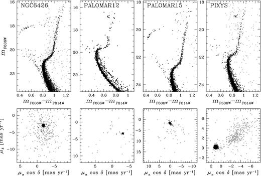
mF606W versus mF606W − mF814W CMDs (upper panels) and vector-point diagrams of proper motions (lower panels) of NGC 6426, Palomar 12, Palomar 15, and Pyxis. Candidate cluster members and field stars are coloured black and grey, respectively.
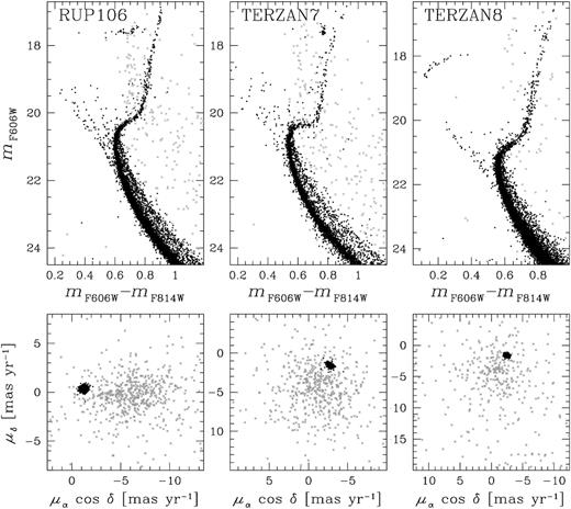
As in Fig. 1 but for Ruprecht 106, Terzan 7, and Terzan 8.
2.2 Stellar models
We exploited the stellar-evolution models and the isochrones used by T20, which have been computed with the stellar-evolution program aton 2.0 (Ventura et al. 1998; Mazzitelli, D’Antona & Ventura 1999). The grid of models used in this paper includes different ages, metallicity (Z), and helium mass fractions (Y). Specifically, the iron abundance ranges from [Fe/H] = −2.44 to −0.45 and the adopted values for [|$\rm \alpha$|/Fe] are 0.0, +0.2, and +0.4. In particular, the models with [|$\rm \alpha$|/Fe] = +0.0 have been calculated specifically for this work. The HB models include a small correction to their helium mass fraction to account for the first dredge up effects. The HB evolution is followed until the end of the helium-burning phase. Gravitational settling of helium and metals is not included.
To derive the RGB mass-loss of each cluster we compare the CMD of the observed HB stars with a grid of synthetic CMDs, obtained following the recipes of D’Antona et al. (2005, and references therein). Briefly, the mass of the each HB star (|$\rm \mathrm{ \mathit{ M}}^{HB}$|) in each simulation is obtained as: |$\rm \mathit{ M}^{HB}=\mathit{ M}^{Tip}(\mathit{ Z}, \mathit{ Y}, \mathit{ A}) - \Delta \mathit{ M}(\mu ,\delta)$|. Here, |$\rm \mathit{ M}^{Tip}$| is the stellar mass at the RGB tip, which depends on age (A), metallicity (Z), and helium content (Y); |$\rm \Delta \mathit{ M}$| is the mass lost by the star and described by a Gaussian profile with central value μ and standard deviation δ.
Once the value of |$\rm \mathit{ M}^{HB}$| is obtained, the star is placed on its HB track via a series of random extraction and interpolation procedures. Each simulation in the grid is composed of few thousands star to avoid problems due to high variance. The values of |$\rm \mathit{ M}^{Tip}$| are obtained from the isochrones that provide the best fit with the observed CMD. We refer to D’Antona et al. (2005), Tailo et al. (2016), and T20 for additional details on the procedure.
3 CONSTRAINING THE RGB MASS-LOSS
In this section, we summarize the procedure to derive the RGB mass-loss in simple-population clusters, using Palomar 15 as a template. After extending the same analysis to the other analysed GCs, we will discuss the results.
3.1 Example case: Palomar 15
To infer the RGB mass- loss experienced by HB stars we follow the procedure introduced by T20 (see also Tailo et al. 2019a, b) and illustrated in Fig. 3 for Palomar 15. This procedure is based on the comparison between the observed HB stars and a grids of simulated HBs.
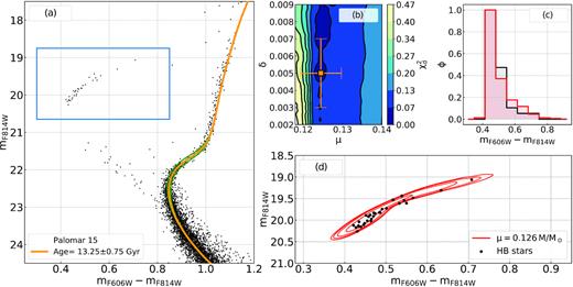
Summary of the procedure we follow to obtain the RGB mass-loss for Palomar 15. In the panel (a), we compare the observed CMD of cluster member with the best-fitting isochrone (yellow line) and the isochrones with ages of ±1σ Gyr from the best age estimate (green line). The blue rectangle highlights HB stars. Panel (b) shows the |$\rm \chi ^2_d$| density plot in the mass-loss dispersion versus mass-loss plane. The best-fitting values are marked by the orange square. The histograms of the colour distribution of observed (black) and simulated HB stars are shown in panel (c), while panel (d) shows the observed HB and contours corresponding to the best-fitting simulated HB (see text for details).
At odds with T20, who studied clusters with multiple populations, our sample consists in candidate simple-population GCs. Hence, we assumed that all their stars have the same chemical composition and adopted pristine helium mass fraction for all clusters.
The first step is to evaluate the age of the population, needed as input to generate the synthetic HB grids. We do that via the isochrone fitting of the turn-off region. We produce an array of isochrones with [Fe/H] = −2.07, [|$\rm \alpha$|/Fe] = + 0.4 (following the indication by Kirby, Guhathakurta & Sneden 2008), and Y = 0.25, with age ranging from 8.0 to 14.0 Gyr in steps of 0.25 Gyr. We adopt E(B− V) = 0.40 and (m− M)V = 19.51 from the 2010 version of the Harris (1996) catalogue.3
The isochrone that provides the best match with the turn-off region in the |$\rm \mathit{ m}_{\mathit{ F}814\mathit{ W}}$| versus |$\rm \mathit{ m}_{\mathit{ F}606\mathit{ W}}-\mathit{ m}_{\mathit{ F}814\mathit{ W}}$| CMD (orange isochrone in Fig. 3a) gives us the best estimate for cluster age, in this case 13.25 ± 0.75 Gyr. The uncertainty corresponds to the age range that allows the isochrones to envelope 68.27 per cent of stars in the turn-off region.
We verified that our age estimate is not significantly affected by unresolved binaries and blue stragglers (BSS). To investigate the possible effect of binaries and BSSs on the inferred cluster ages, we simulated two mock CMDs of Palomar 15 with the same age and metallicity values adopted here, but different fraction of binaries and BSSs. In the first CMD, we assumed no binaries and BSSs, while in the second one, the same fraction of binaries derived by Milone et al. (2016) and the same number of BSSs as observed in the actual CMD. We derive the GC age of both simulated CMDs by using the same methods described above and we obtain that the age values are consistent within 0.25 Gyr. Hence, we conclude that binaries and BSSs do not affect our age determination.
Our second step is to identify, by eye, the HB stars in the cluster. The selected HB stars of Palomar 15 are enclosed in the blue rectangle of Fig. 3(a). We take extra care to verify that the stars are identified on the HB in both |$\rm \mathit{ m}_{\mathit{ F}814\mathit{ W}}$| versus |$\rm \mathit{ m}_{\mathit{ F}606\mathit{ W}}-\mathit{ m}_{\mathit{ F}814\mathit{ W}}$| and |$\rm \mathit{ m}_{\mathit{ F}606\mathit{ W}}$| versus |$\rm \mathit{ m}_{\mathit{ F}606\mathit{ W}}-\mathit{ m}_{\mathit{ F}814\mathit{ W}}$| CMDs.
The selected HB stars are compared with appropriate grids of simulated HBs corresponding to different values of mass-loss (μ) and mass-loss dispersion (δ; see T20 for details). In the case of Palomar 15 |$\rm \mu$| varies from 0.010 to 0.180 |$\rm M_\odot$| in steps of 0.003 |$\rm M_\odot$|, and δ ranges from 0.002 to 0.009 |$\rm M_\odot$| in steps of 0.001 |$\rm M_\odot$|.
For each simulation in the grid, we compare the normalized histogram of the colour distribution of observed and simulated stars. To quantify the goodness of the fit, we calculate the χ-squared distance between the two histograms, |$\rm \chi ^2_d$| (see Dodge 2008 and T20). The resulting density map of |$\rm \chi ^2_d$| values in the |$\rm \mu$| versus δ plane is plotted in Fig. 3(b). The best-fitting simulation is then the one that minimizes the |$\rm \chi ^2_d$| and is indicated with the orange square on the map of Fig. 3(b).
We evaluate the uncertainty on our estimates of mass-loss and mass-loss dispersion by means of bootstrapping. We generated 5000 realizations of the HB in Palomar 15 and performed the comparison with the grid of simulated HBs on each iteration. To estimate the uncertainties on mass-loss and mass-loss dispersion we first considered the standard deviation of the results.
Moreover, we added the contribution to the error from the uncertainties on cluster age, metallicity, and reddening. To do this, we derived mass-loss by using the same procedure above but by changing cluster age by 0.75 Gyr, iron abundance by 0.10 dex, and reddening by E(B− V) = 0.015 mag. In clusters without spectroscopic determination of α-element abundance, we also accounted for the effect of a variation in [α/Fe] by 0.2 dex. By adding in quadrature all the contributions to the total error, we obtain the final estimate for the mass-loss of Palomar 15: |$\rm \mu =0.126\pm 0.030 \,M_\odot$|.
The best-fitting isochrone provides the mass at the RGB tip, |$\rm \mathit{ M}^{Tip} = 0.783\, M_\odot$| and for the HB stars (|$\rm \mathit{ M}^{HB} = 0.674 \pm 0.030\, M_\odot$|). The complete list of parameters inferred from the procedure illustrated for Palomar 15 are listed in in Table 2 for all studied clusters.
For completeness, we compare the histogram of the colour distribution of the best-fitting simulation, i.e. the one whose values of |$\rm \mu$| and |$\rm \delta$| minimize |$\rm \chi ^2_{d}$|, with the corresponding histogram from observed HB stars (Fig. 3c). Finally, in the panel (d) of Fig. 3, we superimposed on the observed CMD, the contours of the best-fitting simulation. In the panel 3(d), the contour lines delimit the regions of the simulated CMD including (starting from the outermost region) 98, 95, 80, and 60 per cent of stars.
4 MASS-LOSS AND HB MASS IN CANDIDATE SIMPLE-POPULATION GCs
The procedure from T20, summarized in the previous section, has been extended to the entire sample of 11 Galactic GCs that are candidate to host a simple stellar population.
The analysed GCs are listed in Table 2, together with the values of [Fe/H], [|$\rm \alpha$|/Fe], E(B− V), and (m− M)V used for their analysis. Specifically, the values of reddening and distance modulus are from the 2010 version of the Harris (1996) catalogue, while the values of [Fe/H] and [|$\rm \alpha$|/Fe] are taken from various literature sources and are derived from spectroscopy (see Table 2 for the complete list of references).
Since no spectroscopic determination for α elements are available for AM 4, Palomar 15, and Pyxis, we fixed the [α/Fe] values based on their metallicity as suggested by Kirby et al. (2008). Hence, we assumed [α/Fe] = 0.2 for AM 4, [α/Fe] = 0.4 for Palomar 15 and [α/Fe] = 0.2 for Pyxis. We also include in the error budget for these clusters the effects of a possible shift of 0.2 in [α/Fe] that stems from the results of Kirby et al. (2008).
The complete showcase of examined HBs with their best-fitting simulations is plotted in Fig. 4, while the values of |$\rm \mu$|, |$\rm \delta$|, and |$\rm \mathit{ M}^{HB}$| derived from the analysis described in Section 3.1 are listed in Table 2.
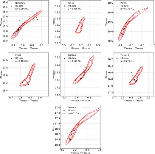
The analysed GCs in alphabetical order. We report in each panel, the |$\rm \mathit{ m}_{\mathit{ F}814\mathit{ W}}$| versus |$\rm \mathit{ m}_{\mathit{ F}606\mathit{ W}}-\mathit{ m}_{\mathit{ F}814\mathit{ W}}$| CMD of the HB stars together with the contour plot of the best-fitting simulation. The average mass-losses of the best-fitting simulations are quoted in the insets.
![Mass-loss ($\rm \mu$) of the HB stars in the simple population GCs as function of their [Fe/H] values. The red line is the best-fitting straight line. In the background, we plot as orange and blue points the mass-loss of the 1G stars for the M3- and M13-like GCs from T20, respectively, and their best-fitting lines. The black dashed line is the general relation from T20.](https://oup.silverchair-cdn.com/oup/backfile/Content_public/Journal/mnras/503/1/10.1093_mnras_stab568/1/m_stab568fig5.jpeg?Expires=1750444504&Signature=rhed3qw8TYVKiSamoMu2UtrYfp~QE1hlh-3Yq2OokLhvF5kbgn3clJMW2VzRzXl4ypRy8U45KhHJa9jp~IsCIihATw~MKKMJVPdnPw7xxrWcZN4umv0WbsSNZ-VtNbSz-1pePECF6FXdk9H4j7mMa-h5I3YKJxJ-ohBdZJCCIe7xHfDFeNnu1QYOMT6w5TQK7G5Fz0COwUDWLC-B9jMdin7wzUJ5uusPaWi~R9msih9jJQuokEJTI7DqFkP0jeLDswjtNJGTSQi7rocR4fazAgVQXi3Inm85IHR1yf0xx21JUyOTeSBS01T0z8N-5~MuP84XShIxilTHo4U1tn4e6A__&Key-Pair-Id=APKAIE5G5CRDK6RD3PGA)
Mass-loss (|$\rm \mu$|) of the HB stars in the simple population GCs as function of their [Fe/H] values. The red line is the best-fitting straight line. In the background, we plot as orange and blue points the mass-loss of the 1G stars for the M3- and M13-like GCs from T20, respectively, and their best-fitting lines. The black dashed line is the general relation from T20.
Linear fits in the form |$\rm \alpha \times [Fe/H] + \beta$| derived in this paper for candidate simple-population GCs and by combining the results of T20 on mass-loss of 1G stars in 46 GCs and those of this paper. We also provide the Pearson rank coefficient, |$\rm \mathit{ R}_P$|, and the r.m.s of the residuals with respect to the best-fitting line.
| Var. | |$\rm \alpha$| | |$\rm \beta$| | |$\rm \mathit{ R}_P$| | Scatter |
|---|---|---|---|---|
| Simple-population GCs | ||||
| |$\rm \mu$| | 0.090 ± 0.013 | 0.301 ± 0.026 | 0.93 | 0.019 |
| |$\rm \mathit{ M}^{HB}$| | 0.002 ± 0.013 | 0.688 ± 0.022 | -0.89 | 0.027 |
| Entire sample | ||||
| |$\rm \mu$| | 0.095 ± 0.006 | 0.312 ± 0.011 | 0.89 | 0.029 |
| |$\rm \mathit{ M}^{HB}$| | −0.026 ± 0.007 | 0.619 ± 0.013 | -0.33 | 0.034 |
5 A UNIVERSAL MASS-LOSS LAW FOR POPULATION II STARS?
In their recent paper, T20 constrained the RGB mass-loss of the distinct stellar populations of 46 galactic GCs with multiple populations. In particular, they investigated the mass-loss of 1G stars and find a linear relation between the RGB mass-loss and the iron abundance of the host GC. The comparison between the findings of our paper and the results from Tailo and collaborators for 1G stars (Fig. 5) reveals that simple-population clusters follow a similar distribution in the mass-loss metallicity plane as 1G stars of multiple-population GCs. In particular, the best-fitting line of simple-population GCs described by equation (1) is almost coincident with the corresponding relation discovered by T20 for the entire sample of 1G stars, |$\rm \mu = (0.095\pm 0.006) \times [Fe/H] + (0.313\pm 0.011)\, M_\odot$|, black dashed line of Fig. 6. In contrast, the RGB mass-loss of simple-populations clusters do not match that of 2G stars with extreme helium contents in GCs with similar metallicities.
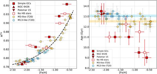
Stellar mass at the tip of the RGB (|$\rm \mathit{ M}^{Tip}$|, left-hand panel) and cluster age (right-hand panel) against iron abundance. Clusters with no HB stars are indicated with open squares, while the other symbols are the same as in Fig. 5. The black dashed line plotted in the right-hand panel is the least-square fit for all T20 clusters, whereas the orange and azure dashed horizontal lines in the right-hand panel indicate the average ages of M 3 and M 13-like GCs, respectively. The corresponding 1 − σ age intervals are indicated by the shaded areas.
This evidence suggests that the relation between mass-loss and metallicity by T20 does not depend on the presence of multiple populations in GCs but may be a standard stellar evolutionary property. This conclusion is corroborated by the results by Salaris et al. (2013) and Savino et al. (2019) who found a similar mass-loss law in dwarf galaxies. By combining the results by T20 for 1G stars in 46 GCs and those in this paper for simple-population clusters we derive the improved relation: |$\rm \mu = (0.095\pm 0.006) \times [Fe/H] + (0.312 \pm 0.011)\, M_{\odot }$|, where the dispersion is ∼0.03 |$\rm M_\odot$| and the correlation coefficients are |$\rm \mathit{ R}_s \sim \mathit{ R}_p\sim 0.89$|. As a matter of fact this is equal to the general relation in T20 (black-dashed line in Fig. 5). We report this general relation in Table 3.
Recent works, based on asteroseismology, provide mass-loss estimates in star clusters. Miglio et al. (2016) used Kepler data of seven RGB and one red-HB stars of the GC M 4 to derive stellar masses. The resulting mass-loss, estimated as the mass difference between HB and RGB stars, ranges from ∼0.0 to ∼0.2 M⊙, depending on the adopted scaling relation. The latter value alone is consistent with the mass-loss inferred by T20 for the 1G stars of M 4.
On the other hand, similar studies on the old, metal-rich open cluster NGC 6791 suggest a moderate RGB mass-loss for this Galactic open cluster (μ = 0.09 ± 0.03 (random) ±0.04 (systematic), Miglio et al. 2012, and references therein), whereas RGB and red clump stars of the ∼2.5 Gyr old cluster NGC 6819 are consistent with sharing the same masses (see also Handberg et al. 2017).
Both NGC 6791 and NGC 6819 ([Fe/H]≥ + 0.3 and [Fe/H]∼0.0, respectively) are more metal rich than the GCs studied in this paper, thus preventing us from a proper comparison. However, we note that the mass-losses inferred by Miglio and collaborators for NGC 6791 and NGC 6819 are much smaller than those of most metal-rich GCs. This difference may imply that the relation between mass-loss and metallicity inferred for GCs cannot be extrapolated to Population I stars, being valid up to [Fe/H] ∼ −0.5. As an alternative, uncertainties in stellar evolution models and/or in asteroseismology scale relations can contribute to the discrepancy between the results based on Kepler data and those of this paper.
5.1 Mass-loss as second parameter of the HB morphology
T20 identified two groups of GCs with different HB morphology: a group of GCs, that, similarly to M 3, exhibit the red HB (M 3-like GCs) and the group of M 13-like GCs with the blue-HB alone (see also Milone et al. 2014). M 3-like and M 13-like GCs are represented with orange and azure colours, respectively, in Fig. 5. The two groups of M 3-like and M 13-like GCs define distinct trends in the μ versus [Fe/H] plane, with M 13-like clusters having higher values of μ1G than M 3-like clusters with similar iron content.
Clearly, the best-fitting line of simple-population clusters is in agreement within 1σ with the corresponding relation of M 3-like GCs [|$\rm \mu = (0.094\pm 0.007) \times [Fe/H] + (0.302\pm 0.011)$|, orange line], but exhibits a different slope than the best-fitting line defined by M 13-like GCs.
To further investigate HB stars in simple-population GCs we show in the left-hand panel of Fig. 6 the stellar mass at the RGB inferred from the best-fitting isochrone against metallicity. In this figure, we also included the studied clusters with no HB stars. Clearly, candidate-simple population GCs exhibit higher values of Mtip than GCs of similar metallicity.
The large RGB-tip stellar masses are mostly due to the fact that the majority of the simple-population clusters are younger than the bulk of GCs studied by T20. This is illustrated in the right-hand panel of Fig. 6 where we show the age–metallicity relation for the clusters studied in this paper (squares) and by T20 (circles).
We confirm previous result by Dotter et al. (2010, 2011, and references therein) and Leaman, VandenBerg & Mendel (2013, and references therein) of two main branches of clusters in the age versus [Fe/H] diagram, with simple population GCs populating the younger branch. From the comparison between observed GC ages and simulations of Milky Way formation, Dotter and collaborators suggested that the distinct branches of clusters in the age–metallicity plane may originate from two different phases of Galaxy formation, including a rapid collapse followed by a prolonged accretion (see also Kruijssen et al. 2019). Similarly, based on the integrals of motions by Massari, Koppelman & Helmi (2019) and Milone et al. (2020) suggested that simple-population GCs may form in dwarf galaxies that have been later accreted by the Milky Way. The possibility in situ and accreted clusters shows similar mass-loss–metallicity relations further corroborates the evidence of a universal mass-loss law.
Candidate simple-population GCs share similar HB masses as shown in Fig. 7, where we plot |$\rm \mathit{ M}^{HB}$| against [Fe/H]. The HB-mass range of candidate simple-population GCs is comparable with that of 1G stars in M 3-like GCs and significantly differs from the behaviour of M 13-like GCs.
![Average HB mass ($\rm \bar{\mathit{ M}}^{HB}$) as a function of [Fe/H] values for clusters studied in this paper and by T20. The symbols and the colour coding are the same as in Fig. 5. Red, orange, and azure continuous lines are the straight lines that provide the best fit with simple-population candidate, M 3 like and M 13-like GCs. The black-dashed line refers to all clusters studied by T20.](https://oup.silverchair-cdn.com/oup/backfile/Content_public/Journal/mnras/503/1/10.1093_mnras_stab568/1/m_stab568fig7.jpeg?Expires=1750444504&Signature=isQJ7KNDOjcjmT95sd62ukZJDH9v84mRUin6ZOltpOhij9lXH5Uco0ZvQVzY9iZQw2at--TOCCL5ZgQClLRKJnKTYKVA~LlAL8yETl29wUT9SyUW2wRcpYOGfVkH6UFs3aArLSfupHe5iT8I0SICCzdBp5PWF8yiaUnp8GkQPTEeaYWrJ-7DTgIyyfyTKfeEZF0kjEaZ50RL~6OZHDOK2SV~HT5HJQD1igcCtvO~h-7H0xAyIFwZi3KWYdTnISZUQWVsxK0JZYQdfQ2AIIAIkHtMQnYZq4PnNyiM3i0jg5Ssm7wNAXRDSEfMiupxLYR68Q4HgNqoPPxXPZynVfx-Bw__&Key-Pair-Id=APKAIE5G5CRDK6RD3PGA)
Average HB mass (|$\rm \bar{\mathit{ M}}^{HB}$|) as a function of [Fe/H] values for clusters studied in this paper and by T20. The symbols and the colour coding are the same as in Fig. 5. Red, orange, and azure continuous lines are the straight lines that provide the best fit with simple-population candidate, M 3 like and M 13-like GCs. The black-dashed line refers to all clusters studied by T20.
The evidence that M 13-like GCs exhibit different patterns than simple-population star clusters in both the μ versus [Fe/H] and the |$\rm \mathit{ M}^{HB}$| versus [Fe/H] planes indicates that their 1G stars behave differently than the bulk of stars with similar metallicity. As a consequence, in addition to metallicity, some second parameter is responsible for the different mass-loss required in their 1G stars. Although M 13-like GCs are, on average, older than M 3-like GCs, age difference alone is not able to account for the different HB shapes. Results of this paper, and from T20, indicate that either mass-loss is the second parameter of the HB morphology or 1G stars of all GCs share the same mass-loss, but the reddest stars of M 13-like GCs are enhanced by 0.01–0.03 in helium mass fraction with respect to M 3-like ones. In this case, as suggested by D’Antona & Caloi (2008), M 13-like GCs could have lost all 1G stars and their red HB tails are populated by 2G stars with moderate helium enhancement.
6 SUMMARY AND CONCLUSIONS
We derived high-precision ACS/WFC photometry in the F606W and F814W of seven GCs that are candidates simple stellar populations. We identified probable cluster members by means of stellar proper motions and corrected the photometry for the effects of differential reddening. The resulting CMDs have been used to infer the RGB mass-loss by comparing the observed HB stars with appropriate simulated CMDs. The main results can be summarized as follows:
The RGB mass-loss in candidate simple-population GCs varies from cluster to cluster and strongly correlates with the cluster metallicity.
The mass-loss versus [Fe/H] relation is consistent with a similar relation inferred by T20 for 1G stars of 46 GCs. We combined the results from this paper and those derived from 1G stars by T20 to derive an improved mass-loss metallicity relation. Moreover, our relation matches the values of mass-loss inferred by Savino et al. (2019) for dwarf galaxies but is not consistent with the mass-losses values inferred for 2G stars by T20.
For a fixed metallicity, the mass-losses and the average HB masses of 1G stars in a subsample of GCs with the blue HB alone (M 13-like GCs) significantly differ from those inferred from simple-population GCs and from 1G stars of the remaining GCs (M 3-like GCs).
These results suggest that the tight correlation between the amount of RGB mass-loss and [Fe/H] that we observed both in simple-population GCs and in 1G stars of multiple-population GCs does not depend on the multiple-population phenomenon and is a good candidate as a general property of Populations II stars. Moreover, the finding that M 13-like GCs exhibit different mass-loss versus metallicity relation than simple-population clusters suggests that mass-loss is one of the main second parameters that govern the HB morphology of GCs.
ACKNOWLEDGEMENTS
This work has received funding from the European Research Council (ERC) under the European Union’s Horizon 2020 research innovation programme (Grant Agreement ERC-StG 2016, No 716082, ‘GALFOR’, PI: Milone, http://progetti.dfa.unipd.it/GALFOR). MT, APM, and ED acknowledge support from MIUR through the FARE project R164RM93XW SEMPLICE (PI: Milone). MT, APM, and ED have been supported by MIUR under PRIN program 2017Z2HSMF (PI: Bedin). EV acknowledges support from NSF grant AST-2009193.
DATA AVAILABILITY
The images analysed in this work are publicly available one the Space Telescope Science Institute HST web page (https://www.stsci.edu/hst) and on the Mikulski Archive for Space Telescopes portal (MAST, https://archive.stsci.edu/). The photometric and astrometric catalogs underlying this article will be released on the Galfor project web page (http://progetti.dfa.unipd.it/GALFOR/) and on the CDS site. The models obtained via the aton 2.0 code are not yet available to the public but they can be provided upon request.
Footnotes
The photometric and astrometric catalogues will be available at the http://progetti.dfa.unipd.it/GALFOR web page and at the CDS (cdsarc.u-strasbg.fr).
