


ABSTRACT
We present the results of numerically solving the rate equations for the first 31 rotational states of CS in the ground vibrational state to determine the conditions under which the J = 1 − 0, J = 2 − 1, and J = 3 − 2 transitions are inverted to produce maser emission. The essence of our results is that the CS(|$\upsilon \!=\!0$|) masers are collisionally pumped and that, depending on the spectral energy distribution, dust emission can suppress the masers. Apart from the J = 1 − 0 and J = 2 − 1 masers, the calculations also show that the J = 3 − 2 transition can be inverted to produce maser emission. It is found that beaming is necessary to explain the observed brightness temperatures of the recently discovered CS masers in W51 e2e. The model calculations suggest that a CS abundance of a few times 10−5 and CS(|$\upsilon \!=\!0$|) column densities of the order of |$10^{16}\, \mathrm{cm^{-2}}$| are required for these masers. The rarity of the CS masers in high-mass star-forming regions might be the result of a required high CS abundance as well as due to attenuation of the maser emission inside as well as outside of the hot core.
1 INTRODUCTION
Molecular maser emission has always been a fascinating phenomenon associated with various astrophysical environments such as evolved stars, star-forming regions, and supernova remnants. As for high-mass star-forming regions, this has been particularly emphasized over the last two decades through the discovery of periodic class II methanol, formaldehyde, and OH masers associated with high-mass star-forming regions (see eg. Goedhart, Gaylard & van der Walt 2003, 2004; Araya et al. 2010; Goedhart et al. 2014, 2019; Szymczak, Wolak & Bartkiewicz 2015; Szymczak et al. 2016, 2018; Sugiyama et al. 2017; Olech et al. 2019). More recently water and methanol maser flaring events associated with high-mass star-forming regions attracted significant attention as such flaring events might be associated with episodic accretion outbursts (Brogan et al. 2018; Szymczak et al. 2018). The periodic masers and maser flaring events are just two examples which illustrate how masers can reveal changes in the star-forming environment which otherwise would not be detected with thermal line emission.
While widespread masers such as e.g. H2O and CH3OH are useful in studying some aspects of high-mass star-forming regions, rare masers, on the other hand, must reveal something special about the star-forming regions with which they are associated. Amongst those masers for which until recently only a single detection has been reported is that of CS. In the course of studying vibrationally excited emission from the carbon-rich giant IRC +10216, Highberger et al. (2000) noted that the CS(|$\upsilon \!=\!1$|) J = 3 − 2 transition has two components with exceptionally small linewidths of, respectively, 1.1 and 2.5 |$\mathrm{km\, s^{-1}}$| compared to other lines they detected. In contrast, the linewidths for other molecules reflect the full expansion velocity of 14.5 |$\mathrm{km\, s^{-1}}$| of the gas in IRC+10216. In addition to the small linewidths, the brightness temperature of the CS(|$\upsilon \!=\!1$|) J = 3 − 2 transition was found to be 526 K compared to significantly smaller values for the other transitions of CS. This led Highberger et al. (2000) to conclude that non-LTE conditions affect the CS (|$\upsilon \!=\!1$|) J = 3 − 2 transition and that it might be a weak maser.
Recently, Ginsburg & Goddi (2019) reported the first discovery of maser emission for the CS(|$\upsilon \!=\!0$|) J = 1 − 0 and J = 2 − 1 transitions associated with a high-mass young stellar object, viz. W51 e2e. Although the observed linewidths for the two masers of, respectively, 7.3 and 5.3 |$\mathrm{km\, s^{-1}}$| were determined by the experimental velocity resolution, both transitions have brightness temperatures of about 6700 K which rules out local thermodynamic equilibrium (LTE) excitation. The two masers were found to be spatially separated by about 190 au and spectrally by about 30 |$\mathrm{km\, s^{-1}}$|. Ginsburg & Goddi (2019) also imaged all three hot cores in the W51 A region in the CS(|$\upsilon \!=\!1$|) J = 1 − 0 transition with a sensitivity of 1.1 mJy beam−1 but did not detect it. This suggests that the physical environment of the CS(|$\upsilon \!=\!0$|) J = 1 − 0 and J = 2 − 1 masers in W51 e2e is such that excitation to the |$\upsilon \!=\!1$| state is either weak or completely absent.
This detection of CS maser emission associated with a very young high-mass star raises the questions of what the pumping mechanism is and why these masers are so rare. The aim of this paper is first to investigate the pumping mechanism and based on that consider why these masers seem to be rare. We restrict our investigation here to the CS(|$\upsilon \!=\!0$|) masers in W51 e2e, leaving the case of the |$\upsilon \!=\!1$| masers, as in IRC +10216, for later follow-up work.
2 NUMERICAL METHOD AND MOLECULAR DATA
The maser region is assumed to be embedded in or surrounded by a layer of warm dust at temperature Td. We assume that the dust radiation field is given by Iν = τd(ν)Bν(Td) with Bν(Td) the Planck function and τd(ν) = τd(ν0)(ν/ν0)p the dust optical depth where we have set |$\tau _\mathrm{ d}(\nu _0=10^{13}\, \mathrm{Hz}) = 1$| (see e.g. Pavlakis & Kylafis 1996; Sobolev, Cragg & Godfrey 1997; Cragg, Sobolev & Godfrey 2002). We note that for dust emission Sobolev et al. (1997) and Cragg et al. (2002) used Iν ∝ [1 − exp (− τd)]Bν(Td) which, in the optically thin case is equivalent to (ν/ν0)pBν(Td).
We solve the rate equations using a fourth-order Runge–Kutta method, which is more accurate and stable than Heun’s method which was used in van der Walt (2014). The initial distribution of the level populations was a Boltzmann distribution with a temperature equal to the average of the dust and kinetic temperatures. For a given |$\mathrm{n_{H_2}}$|, the calculation started with a small CS specific column density such that the system is completely optically thin in all transitions. An equilibrium solution for this initial specific column density was then found by letting the system evolve in time-steps of 0.5 s till the convergence condition |Ni(tj + 1) − Ni(tj)|/Ni(tj) < 10−6 is reached for all levels i. The specific column density is then increased by a small amount with the equilibrium solution for the previous value of the specific column density being used as the initial distribution. The process is repeated until the required specific column density is reached.
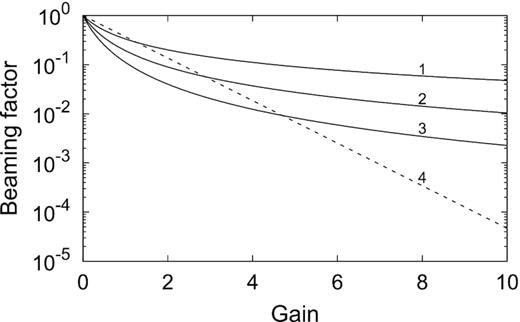
Comparison of the variation of the beaming factor for the four different dependencies of Ω/4|$\pi$| on the gain: (1) (2τ + 1)−1, (2) (2τ + 1)−1.5, (3) (2τ + 1)−2, and (4) 10−0.433τ.
The Einstein-A and collisional rate coefficients of the first 31 levels of CS were taken from the Leiden Atomic and Molecular Database (Schöier et al. 2005). The collisional rate coefficients were extrapolated from 300 to 500 K using equation (13) of Schöier et al. (2005) to allow also for the possibility of higher gas kinetic temperatures than what is given on the Leiden Atomic and Molecular Database.
3 RESULTS
As explained in the previous section, the calculational procedure to find the equilibrium solution for a given combination of |$\mathrm{n_{H_2}}$|, Tk, Td, and CS specific column density is to start at a small specific column density where the system is optically thin, and to evolve the system in small steps in specific column density. Fig. 2 shows some examples of the variation of the optical depth as the specific column density is increased in steps of 0.01 dex when excitation is through collisions and internal generated radiation only, i.e. the dust radiation field is switched off. All calculations started at a specific column density of |$10^6\, \mathrm{cm^{-3}\, s}$| and ended at |$2\times 10^{12}\, \mathrm{cm^{-3}\, s}$|.
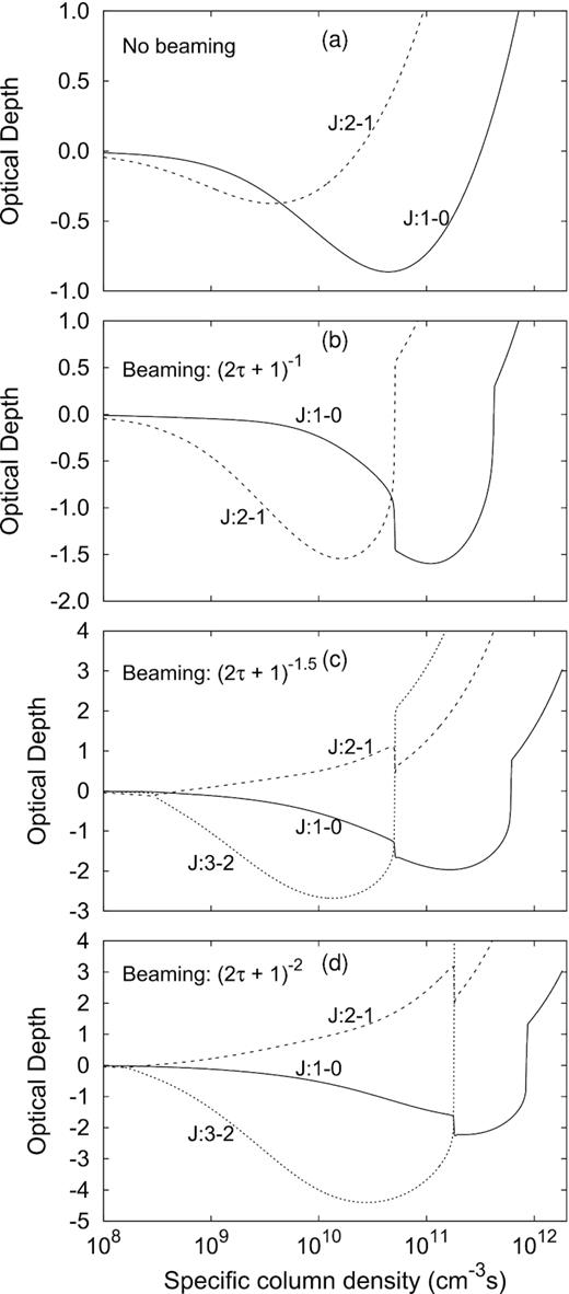
Figure to illustrate how the optical depth changes with specific column density as well as the effect of increased beaming. In all four panels, only collisional excitation was considered. Note in (b) how the J = 1 − 0 transition is affected when the inversion of the J = 2 − 1 transition is lifted. Similar behaviour can also be seen in (c) and (d) where it is shown that the J = 3 − 2 transition is also inverted. Lifting of the inversion in the J = 3 − 2 transition affects both the J = 2 − 1 and J = 1 − 0 transitions. Inversion of the J = 3 − 2 transition occurs only when collisional excitation is the dominant mechanism. Parameter values used: |$\mathrm{n_{H_2}}$| = |$3.7\times 10^{5}\, \mathrm{cm^{-3}}$|, Tk = 300 K.
Panel (a) shows the optical depth as a function of specific column density for the J = 1 − 0 and J = 2 − 1 transitions when there is no beaming. For both transitions, the optical depth decreases toward a minimum value (maximum gain) after which it increases to eventually become positive. While both transitions can be inverted at the same specific column density, the maximum gain for the J = 2 − 1 transition is seen to occur at a smaller specific column density than for the J = 1 − 0 transition. As will be shown later, it is generally the case that the maximum gain for the two masers does not occur at the same specific column density.
Panels (b)–(d) show how the behaviour of the optical depth changes when beaming is introduced. Comparison with panel (a) shows that beaming has a marked effect on how the optical depth changes with specific column density. Panel (b) shows that the specific column density where maximum gain occurs has shifted to larger specific column densities. Also, the maximum gain has increased. Perhaps the most interesting and noteworthy difference with Panel (a) is that the lifting of the inversion for the J = 2 − 1 transition occurs over one step in specific column density. When this happens the gain of the J = 1 − 0 maser increases since population in the J = 1 state ‘suddenly’ increases. This behaviour is quite general since the two masers share the J = 1 state in a single ladder of rotational states.
A further interesting result of increasing the beaming is that the J = 3 − 2 transition also becomes inverted as is seen in panels (c) and (d). Note how now three masers are linked through the J = 1, and J = 2 states. Thus, when the inversion of the J = 3 − 2 transition is lifted, it affects the J = 2 − 1 and the J = 1 − 0 transitions. The inversion of the J = 3 − 2 transition occurs only when collisions dominate the excitation and does not occur at all combinations of |$\mathrm{n_{H_2}}$| and Tk. For most of what follows the focus will be on the J = 1 − 0 and J = 2 − 1 masers in the ground vibrational state.
The results presented in Fig. 2 show that inversion of the J = 1 − 0 and J = 2 − 1 transitions can be accomplished with collisions as the primary excitation mechanism which implies that the masers are collisionally pumped. An infrared radiation field, however, permeates the star formation environment and it is necessary to examine what the effect of the presence of such a radiation field is. In addition to the temperature of the dust, it is also necessary to consider the effect of geometric dilution. Instead of considering the maser gain, we will henceforth consider the maser brightness temperature, calculated from equation (7), which is more relevant for comparison with observations. The effect of the dust temperature on the brightness temperature is shown in Fig. 3 and that of the geometric dilution in Fig. 4 when the dust spectral energy distribution is that of a blackbody. Increasing the dust temperature results in a decrease in the maser brightness temperature with a similar behaviour when the dilution factor is increased. Note that a dilution factor of zero implies collisions only and a value of one means that the dust emission originates inside the masing region. These results imply that both masers are affected negatively when the dust emission becomes stronger. The case when the dust emissivity is of the more general form (ν/ν0)pBν(Td) will be presented later.
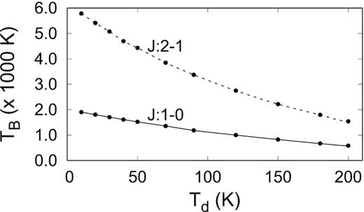
Graph showing how the brightness temperature changes with dust temperature for |$\mathrm{n_{H_2} = 2.5\times 10^5\, \mathrm{cm^{-3}}}$|, Tk = 360 K, and a geometric dilution factor of 0.4. The emissivity of the dust was assumed to be that of a blackbody. The black dots indicate the dust temperatures at which the calculations were done. The solid and dashed lines are smooth fits to the points. The same applies to Fig. 4.
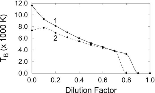
Graph showing how the brightness temperature changes with the geometric dilution of the dust radiation field. (1) For the J = 1 − 0 transition when |$\mathrm{n_{H_2}}$| = |$5 \times 10^4\, \mathrm{cm^{-3}}$|, Tk = 360 K, and Td = 100 K. (2) For the J = 2 − 1 transition when |$\mathrm{n_{H_2}}$| = |$1.6 \times 10^5\, \mathrm{cm^{-3}}$|, Tk = 460 K, and Td = 100 K. For both transitions, the brightness temperatures are only a few Kelvin at the larger dilution factors.
A different representation, which gives a better overall view of the behaviour of the two masers can be obtained by considering the variation of the brightness temperature in the |$\mathrm{n_{H_2}}$|−Tk plane. For this, we considered H2 densities in the range 104 to |$10^6\, \mathrm{cm^{-3}}$| with intervals of 0.1 dex. The kinetic temperature ranged between 30 and 500 K in steps of 10 K between 30 and 300 K and steps of 20 K between 300 and 500 K. This gives a total of 798 samplings in the |$\mathrm{n_{H_2}}$|−Tk plane. Unless stated otherwise, a dust temperature of 100 K and a geometric dilution factor of 0.2 were used. Presenting the model results in this way requires that a single brightness temperature be associated with each combination of |$\mathrm{n_{H_2}}$| and Tk. In what follows, it is therefore assumed that the masers operate at maximum gain, i.e. where the optical depth has its largest negative value. The brightness temperature was calculated using the corresponding level populations at maximum gain for the particular transition. The brightness temperature was set equal to zero when there was no inversion.
In Fig. 5, we show the variation of the brightness temperature when collisions are the only excitation mechanism (infrared radiation field switched off) and with no beaming. It is seen that an inversion can obtained with collisions as the only pumping mechanism over a significant part of the |$\mathrm{n_{H_2}}$|−Tk plane. Both panels suggest that inversions occur also outside the ranges used for |$\mathrm{n_{H_2}}$| and Tk, i.e. for densities greater than 106 cm−3 and Tk > 500 K. For the J = 1 − 0 transition the maximum brightness temperature is 114 and 91 K for the J = 2 − 1 transition. The brightness temperatures for both transitions are significantly smaller than what has been observed by Ginsburg & Goddi (2019). Although the region over which there is an inversion in the J = 2 − 1 transition is completely overlapped by the region over which there is inversion of the J = 1 − 0 transition, it is again noted that the inversions do not occur at the same CS specific column densities as will be discussed later.
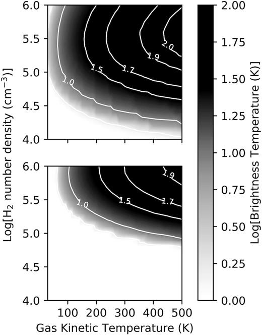
Although radiative excitation alone does not result in inversion for any of the two transitions, the presence of a dust radiation field does have an effect on the inverted level populations as was shown in Figs 3 and 4. Fig. 6 shows the variation of the brightness temperature when the radiation field is that of a 100 K blackbody modified according to the wavelength-dependent escape probability. Comparison with Fig. 5 shows that in the presence of such a radiation field the brightness temperature at a specific (|$\mathrm{n_{H_2}}$|,Tk) point is reduced for both transitions. Also, for both transitions, the region in the |$\mathrm{n_{H_2}}$|−Tk plane where inversion occurs is smaller and is shifted to higher H2 densities.
Contour and grey scale plot of the brightness temperature for the J = 1 − 0 transition (upper panel) and the J = 2 − 1 transition (lower panel) in the |$\mathrm{n_{H_2}}$|−Tk plane in the presence of a blackbody dust radiation field with |$T_{\rm d} = 100\, {\rm K}$| and with no beaming.
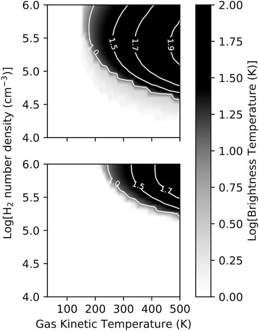
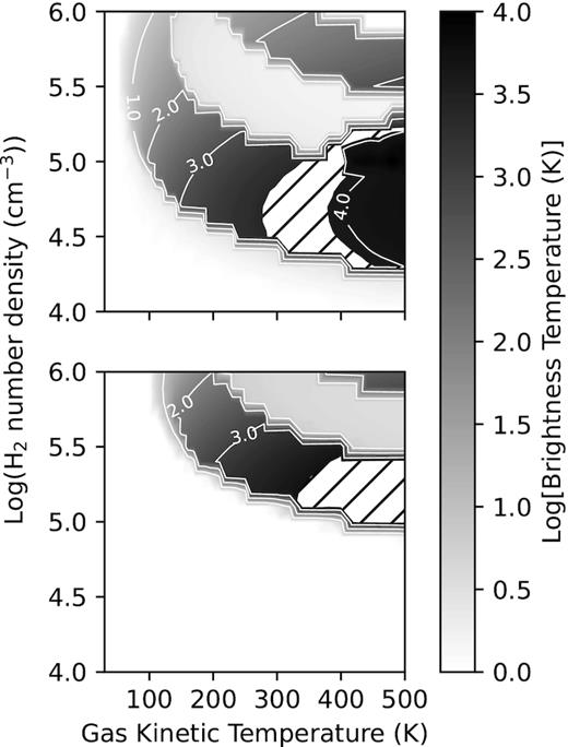
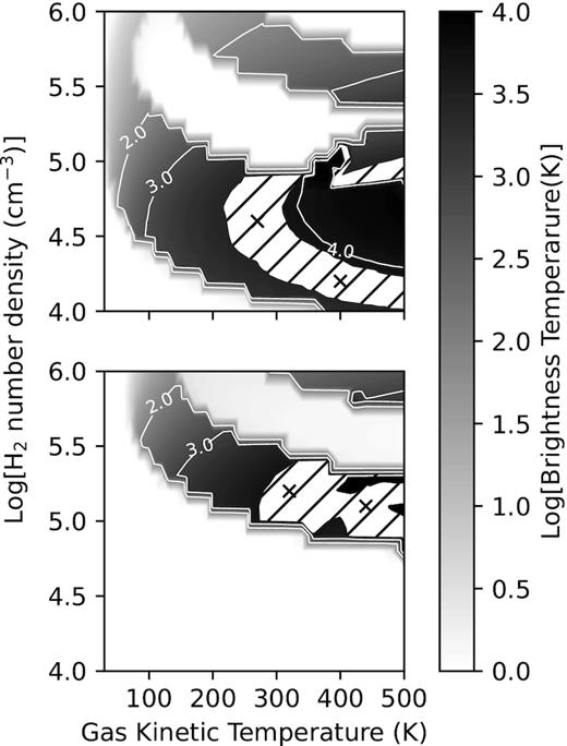
In Figs 7–9, we show the effect of beaming on the maser brightness temperature when Ωij/4|$\pi$| = (2τij + 1)−η. Comparison of Fig. 7 (η = 1) with Fig. 6 shows that not only is the region over which inversion occurs now larger but the brightness temperatures are also higher. However, the maximum brightness temperatures of 593 and 346 K for the J = 1 − 0 and J = 2 − 1 masers, respectively, are still significantly less than what has been observed for W51 e2e. Increasing the beaming further (Fig. 8, η = 1.5) results in significant changes in the shape of the region in the |$\mathrm{n_{H_2}}$|−Tk plane where inversion occurs. In this case, the maximum brightness temperatures for the J = 1 − 0 and J = 2 − 1 masers are 2550 and 1400 K, respectively, which are still too low to explain the observed brightness temperatures of the masers in W51 2e2.
Contour and grey scale plot of the brightness temperature of the J = 1 − 0 transition (upper panel) and the J = 2 − 1 transition (lower panel) in the |$\mathrm{n_{H_2}}$|−Tk plane with beaming factor given by (2τij + 1)−1 for Td = 100 K and a geometric dilution factor of 0.2.
Same as for Fig. 7 but now with the beaming factor given by (2τij + 1)−1.5.
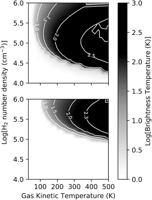
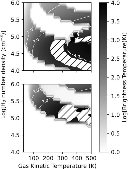
Same as for Fig. 8 but now with the beaming factor given by (2τij + 1)−2. The white filled region indicates the region where the maser brightness temperature lies between 6000 and 8000 K.
The result when Ωij/4|$\pi$| = (2τij + 1)−2 is shown in Fig. 9. The maximum brightness temperatures for the J = 1 − 0 and J = 2 − 1 masers are respectively 24700 K and 8580 K. The white hatched regions show where the brightness temperature for each maser lies between 5000 and 9000 K. For the J = 1 − 0 transition, the region has an arch-like shape and lies more or less between kinetic temperatures 300 and 400 K and |$10^{4.5} \lesssim \mathrm{n_{H_2}} \lesssim 10^5\, \mathrm{cm^{-3}}$|. For the J = 2 − 1 transition, the corresponding values are Tk ≳ 350 K and |$10^5 \lesssim \mathrm{n_{H_2}} \lesssim 10^{5.5}\, \mathrm{cm^{-3}}$|. Fig. 9 shows that with stronger beaming the regions in the |$\mathrm{n_{H_2}}$|−Tk plane where the one maser is significantly brighter than the other become separated. Closer comparison of the upper and lower panels shows that the J = 2 − 1 transition is not inverted over most of the region where the J = 1 − 0 transition is inverted. The J = 1 − 0 transition, on the other hand, is inverted over most of the region where the J = 2 − 1 maser occur but has brightness temperature which is significantly less than that of the J = 2 − 1 maser. Only at the very high1 temperatures is there a small region where there is overlap. It is also seen that there are two regions where the J = 1 − 0 maser can occur, one at H2 densities smaller and one at densities greater than where the J = 2 − 1 maser occur.
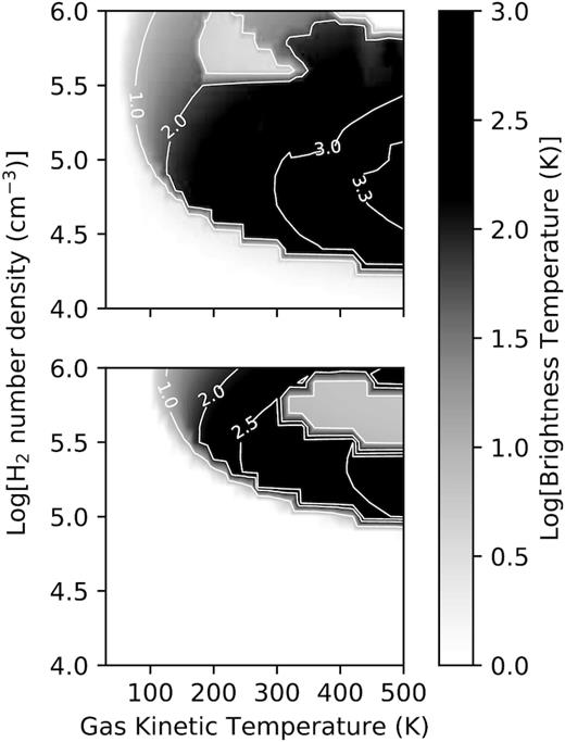
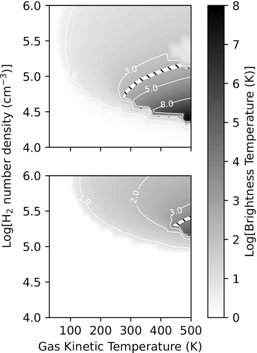
We also considered the case when the dust emissivity has the form (ν/ν0)Bν(Td) with ν0 = 1013 Hz. Fig. 10 shows the result for the same values of the other parameters as for Fig. 9. It is interesting to note that the region over which the J = 1 − 0 transition is inverted is significantly larger compared to the case when it is assumed that the dust emissivity behaves like a blackbody. The arch-like region where 5000 < TB < 9000 for the J = 1 − 0 transition in Fig. 9, now extends down to lower H2 densities and higher kinetic temperatures. To understand this change note that the largest energy difference amongst the 31 levels, i.e. between J = 30 and 29, is equivalent to a frequency of about 1.5 × 10¹² Hz. Having a dust emissivity that varies as (ν/ν0)Bν(Td) with ν0 = 1013 Hz means that the energy density in the radiation field at those frequencies that can affect the level populations, is reduced by more than 15 per cent compared to that of a blackbody emissivity. The effect of this change in the spectral energy distribution is that collisions and spontaneous emission are effectively the only mechanisms that affect the level populations. To confirm this, we also performed calculations when collisions are the only excitation mechanism and with the beaming factor given by (2τij + 1)−2. The result is shown in Fig. 11. The similarity with Fig. 10 is obvious and implies that dust emissivities of the form (ν/ν0)pBν(Td) with 1 ≤ p ≤ 2, which is often used (e.g. Pavlakis & Kylafis 1996, 2000; Cragg et al. 2002), will result in the J = 1 − 0 and J = 2 − 1 masers having the same behaviour as that in Fig. 11.
Same as for Fig. 9 but for a dust emissivity given by (ν/ν0)Bν(Td). The hatched white region indicates the region where the maser brightness temperature lies between 6000 and 8000 K. The four crosses indicate the combinations of Tk and |$\mathrm{n_{H_2}}$| used to estimate CS column densities and abundances.
Same as for Fig. 9 but with no radiation field included. Excitation is therefore purely collisional.
A noticeable feature in Figs 9–11 is the stair-step behaviour which needs some explanation. Closer inspection of the model results shows that at a given kinetic temperature, the brightness temperatures of the J = 1 − 0 and J = 2 − 1 transitions increase significantly with an increase of 0.1 or 0.2 dex from the density where there first is an inversion. For example, in the case of Fig. 11, at Tk = 200 K the J = 1 − 0 transition already has a very weak inversion at H2 densities of 104 and |$10^{4.1}\, \mathrm{cm^{-3}}$| with brightness temperatures of 0.5 and 1.0 K, respectively. Increasing the density to |$10^{4.2}\, \mathrm{cm^{-3}}$| raises the brightness temperature to 2833 K. The same behaviour occurs at 180 K where the brightness temperature changes from 0.8 K at an H2 density of |$10^{4.1}\, \mathrm{cm^{-3}}$| to 2215 K at |$10^{4.2}\, \mathrm{cm^{-3}}$|. At 240 K the increase is from 1.3 to 3300 K. Although there is an increase of about 1000 K in the brightness temperature from Tk = 180 to 240 K at |$\mathrm{n_{H_2}}$| = |$10^{4.2}\, \mathrm{cm^{-3}}$|, such a change is not visible on the contour plots. A contour level of, say, 2000 K for the brightness temperature will therefore occur at the same H2 density for kinetic temperatures between 180 and 240 K in this particular example. The same explanation applies to other kinetic temperature intervals, e.g. from 250 to 340 K, where the maser brightness temperature, as represented by the contours, seems to stay constant. The stair-step effect is therefore a consequence of the 0.1 dex step size in |$\mathrm{n_{H_2}}$| and would have been smaller if a smaller step size was used. We note that such a rapid increase in brightness temperature with a small change in |$\mathrm{n_{H_2}}$| is also seen in the results of Pavlakis & Kylafis (2000) on OH masers.
Considering the results presented in Panels (c) and (d) of Fig. 2 as well as that in Figs 10 and 11, we examined over what region in the |$\mathrm{n_{H_2}}$|−Tk plane the J = 3 − 2 transition is inverted. The result is shown in Fig. 12. Since the inversion occurs only at higher densities the calculations were done for H2 densities greater than 105 cm−3 only and Tk ≥ 100 K. In this particular case, the step size in density was 0.05 dex. Comparison of the two panels shows that the region where the J = 3 − 2 transition is inverted is basically the same as the higher density region (there is also a region at lower densities not shown in this Figure) where the J = 1 − 0 transition is inverted but not the J = 2 − 1 transition. However, as was shown in Fig. 2, the specific column density where the J = 3 − 2 transition has maximum gain is smaller than where the J = 1 − 0 transition has maximum gain. The second point to note is that the brightness temperature of the J = 3 − 2 maser is comparable with that of the J = 1 − 0 and J = 2 − 1 masers observed in W51 e2e, i.e. in excess of several thousand Kelvin. Thus, at least theoretically, these results suggest that, based on the brightness temperature, the J = 3 − 2 maser should be detectable in W51 e2e depending on the presence of gas with densities ∼105.4 to ∼105.8 cm−3 and with kinetic temperatures greater than about 250 K.
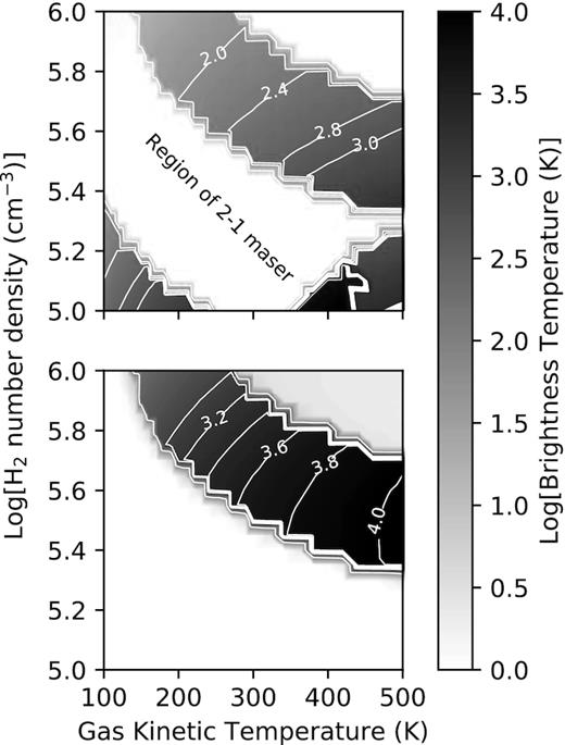
Contour and grey scale plot of the brightness temperature for the J = 1 − 0 transition (upper panel) and the J = 3 − 2 transition (lower panel) in the |$\mathrm{n_{H_2}}$|−Tk plane. The dust temperature was taken as 100 K with the emissivity given by (ν/ν0)1.5Bν(Td) where ν0 = 1013. The beaming factor used was the same as in Fig. 9.
We also considered the case when beaming is taken to be the same as that used by Sobolev et al. (1997). The result is shown in Fig. 13. While to a large extent the distribution in the |$\mathrm{n_{H_2}}$|−Tk plane of where inversion occurs is the same as for the other cases considered, it seen that the maximum brightness temperatures for the J = 1 − 0 and J = 2 − 1 transitions are much higher. In the case of the J = 1 − 0 transition, it exceeds 108 K! For both the J = 1 − 0 and J = 2 − 1 transitions the regions where 5000 ≤ TB ≤ 9000 K are two narrow strips.
Contour and grey scale plot of the brightness temperature for the J = 1 − 0 transition (upper panel) and the J = 2 − 1 transition (lower panel) in the |$\mathrm{n_{H_2}}$|−Tk plane with beaming factor given by |$10^{-0.433\tau _{ij}}$| for Td = 100 K, and geometric dilution factor of 0.2.
It was already noted briefly with regard to Fig. 5, that although there is overlap in the |$\mathrm{n_{H_2}}$|−Tk plane where the J = 1 − 0 and J = 2 − 1 masers occur, these masers have their maximum gains at different specific column densities. This is illustrated in the upper panel of Fig. 14 where the specific column density where the J = 2 − 1 maser has maximum gain is plotted against the specific column density where the J = 1 − 0 maser has maximum gain for those instances where both transitions are inverted. All the points are seen to be located well below the y = x line. Thus, for the case when collisions are the only excitation mechanism and with no beaming, the specific column density where the J = 2 − 1 maser has maximum gain is always less than the specific column density where the J = 1 − 0 maser as its maximum gain. In the bottom panel of Fig. 14 we show the same graph but for the case of Fig. 11, i.e. with the beaming factor of the form (2τij + 1)−2 and collisions as the only excitation mechanism. Refering to Fig. 11, this is the case where there are rather well-defined regions in the |$\mathrm{n_{H_2}}$|−Tk plane where one of the masers is strong and the other one weak or absent or both masers are strong. From the bottom panel of Fig. 14, it is seen that now there are three clearly distinct groups of points. Group A is for the case when the maximum gain and the brightness temperature of the J = 1 − 0 maser are significantly greater than that of the J = 2 − 1 maser. Typically, for group A the brightness temperature of the J = 1 − 0 maser is greater than 100 K while for the J = 2 − 1 maser it is only about 1 or 2 K. Group B is just the opposite of group A, viz. the J = 2 − 1 maser is bright and the J = 1 − 0 maser very weak. For group C both masers have brightness temperatures greater than 1000 K. The location of the three groups relative to the y = x line shows that generally the J = 1 − 0 and J = 2 − 1 masers do not have their respective maximum gains at the same CS specific column density.

Plot of the specific column density where the J = 2 − 1 maser has its maximum gain against the specific column density where the J = 1 − 0 maser has its maximum gain. Upper panel: for collisions only and no beaming (see Fig. 5). Bottom panel: for collisions only and with the beaming factor given by (2τij + 1)−2 (see Fig. 11).
4 DISCUSSION
4.1 General comments
One of the first questions asked about a particular astronomical maser is how it is pumped. In the case of the CS masers the results of the numerical calculations presented above clearly suggest that these masers are pumped collisionally. It was shown that the J = 1 − 0, J = 2 − 1, and J = 3 − 2 transitions can be inverted in the absence of an external radiation field or when the dust emissivity is of the form (ν/ν0)pBν(Td) with 1 ≤ p ≤ 2 and ν0 = 1013 Hz, in which case the emission below 1013 Hz is strongly reduced relative to that of a blackbody. On the other hand, dust emission with a blackbody spectral energy distribution below about 1013 Hz negatively affects the population inversion of these three transitions. Considering all of these results it can be concluded that the CS masers are collisionally pumped.
We also note that there is some qualitative agreement with the observations of Ginsburg & Goddi (2019). These authors found that the J = 1 − 0 and J = 2 − 1 masers are clearly separated spatially and kinematically. Considering the cases where the brightness temperatures of the two masers fall between 5000 and 9000 K (Figs 9 and 10) as well as that the two masers do not have maximum gain at the same specific column densities (Fig. 14) very strongly suggests that the J = 1 − 0 and J = 2 − 1 masers will observationally not be found to be co-spatial.
As pointed out by Ginsburg & Goddi (2019), the newly discovered CS J = 1 − 0 and J = 2 − 1 masers associated with W51 e2e form part of a group of rare masers which raises the question of why these masers are so rare. These authors speculate that W51 e2e may have unique characteristics regarding the infrared radiation field, chemistry, geometry or any other unique aspect that favours CS masers. As for the radiation field, we already noted that brighter masers are produced in an environment with a dust emissivity of the form (ν/ν0)pBν(Td) rather than with a blackbody dust emissivity. However, such a dust emissivity is not unique and cannot be considered as a reason why these masers are rare. Another factor may be the geometry of the masing region which can affect the beaming and therefore the brightness of the masers. It was found that beaming which is stronger than that given by Elitzur (1992) but similar to that found by Spaans & van Langevelde (1992) is needed to explain the observed brightness temperatures of the masers. However, it should not be as strong as that used by Sobolev et al. (1997). On the other hand, W51 e2e also has associated class II methanol masers, which quite generally have very high brightness temperatures and which requires strong beaming. Why a different behaviour of the beaming factor is required for CS and CH3OH masers is not clear.
4.2 Column densities
Two other factors that can play a role in explaining the uniqueness of W51 e2e for favouring CS masers are the CS abundance and column density. We first consider the column density (cm−2) which is found from the CS specific column density where the inversion is maximum and the linewidth. The linewidths given by Ginsburg & Goddi (2019) are basically instrumental linewidths and it can therefore be expected that the real maser linewidths are smaller. Here, we use a linewidth of 1.0 |$\mathrm{km\, s^{-1}}$| for both masers which can be considered as a lower limit. For illustrative purposes, CS column densities were calculated for both masers at two combinations of kinetic temperature and H2 density as indicated by the crosses in Fig. 10. For the J = 1 − 0 maser at Tk = 270 K and |$\mathrm{n_{H_2}}$| = |$10^{4.6}\, \mathrm{cm^{-3}}$|, the column density is found to be log NCS = 15.9. For Tk = 400 K and |$\mathrm{n_{H_2}}$| = |$10^{4.2}\, \mathrm{cm^{-3}}$| the column density is log NCS = 16.1 which, for practical purposes, is the same as for the lower temperature case. For the two combinations for the J = 2 − 1 maser, the CS column density was found to be the same viz. log NCS = 15.6.
These values can be compared with column densities derived by a number of authors using LVG model fitting of observations of high-mass star-forming regions. For 11 northern cores Zinchenko et al. (1994) found 〈log NCS〉 = 13.6. Juvela (1996) did a multitransition study toward 33 southern H2O maser sources and found 〈log NCS〉 = 13.62. Plume et al. (1997) also did a multitransition CS study of 150 high-mass star-forming regions with associated H2O masers. These authors found 〈log NCS〉 = 14.36 for 71 of these regions. Larionov et al. (1999) did a survey of 158 bipolar outflow and methanol maser sources in the Northern sky and give CS column densities for 50 of these sources with 〈log NCS〉 = 14.47. Simply taken at face value, these column densities are at least an order of magnitude less than what is derived from the model calculations. However, it has to be noted that all four of these studies were using single-dish telescopes and that the derived column densities are averages over significantly large regions of the individual star-forming regions observed. For example, the beam size for the observations by Plume et al. (1997) range between 10 and 30 arcsec and for W51 included many unresolved cores for which the CS column densities certainly are higher than the beam averaged values.
4.3 Abundances
As in the case for the column densities, a quantitative comparison of abundances derived from observations with that from the model is not simple for two reasons. First, abundances determined from single-dish observations are, like column densities, averages along the line of sight as well as beam averaged and therefore do not take source structure into account (Wakelam et al. 2004). Secondly, abundances derived from the model results are calculated from the relation |$X_{\mathrm{CS}} \mathrm{n_{H_2}} \ell = \mathrm{N_{CS}}$|, where XCS is the CS abundance relative to H2, ℓ the maser path-length and, NCS is the CS column density calculated from the product of the specific column density where the maser gain is maximum and the maser linewidth (taken as 1 |$\mathrm{km\, s^{-1}}$|). The maser path-length is unknown and the derived CS abundance will therefore depend on the assumed maser path-length. In spite of these limitations, it is nevertheless useful to compare the abundances inferred from the model calculations with some observationally derived values. We first consider CS abundances derived from observations and then maser path-lengths used by other authors.
Dickens et al. (2000) derived CS abundance ranges between 7 × 10⁻¹⁰ and 7 × 10⁻⁹ for the dark cloud L134N. Such low abundance is expected for dark clouds. For the Orion hot core, Chandler & Wood (1997) derived a CS abundance of 1.2 × 10⁻⁸, which is only slightly higher than the maximum CS abundance for L134N. Similar abundances were also found for W43MM1, IRAS18264-1152, IRAS05358+3543, IRAS18162-2048 (Herpin et al. 2009) and AFGL2591 (van der Tak et al. 2003). Bergin et al. (1997) derived CS abundances relative to CO of between 2 × 10⁻⁵ and 1 × 10⁻⁴ for M17 and Cepheus, respectively, which gives CS abundances relative to H2 of the order of 10−8−10−9 using [CO]/[H2] = 10−4 (Kruegel 2003). More recently Barr et al. (2018) derived a CS fractional abundance relative to H2 of 2 × 10⁻⁶ for the hot molecular core associated with the massive protostar AFGL 2591 using mid-infrared spectroscopy. These observations probed the hot gas (∼700 K) which strongly points a higher CS abundance closer to the protostar.
As for maser path-lengths, we note the following. Based on an angular diameter of 0.005 arcsec for OH masers in W3(OH), Moran et al. (1978) inferred a total maser path-length of about 1015 cm for unsaturated OH masers. Reid et al. (1980) similarly concluded that gain lengths of the order of 2 × 1015 cm are required to explain very bright OH masers in W3(OH). Also considering OH masers, Gray, Field & Doel (1992) concluded that long maser path-lengths, i.e. greater than 1014 cm may be composed of a series of regions along the line of sight having similar velocities. These authors also conclude that for OH masers, path-lengths as short as 1013 cm may be adequate to explain observed maser brightness temperatures. Pavlakis & Kylafis (1996) and Pavlakis & Kylafis (2000) used a maser path-length of 5 × 1015 cm for OH masers in star-forming regions. On the other hand, Sobolev et al. (1997) and Cragg et al. (2002) assumed a path-length of 1017 cm in their models for class II CH3OH masers.
In spite of the fact that deriving a CS abundance from the model results depends on an assumed maser path-length, some constraints can be used to put limits on the maser path-length and therefore on the CS abundance. As already noted earlier, the J = 2 − 1 maser is pumped at a higher H2 density compared to the J = 1 − 0 maser which might suggest that the J = 2 − 1 masing region is closer to the exciting star and that the kinetic temperature is also higher than in the masing region of the J = 1 − 0 maser. To take such a scenario approximately into account, we calculated |$\langle \mathrm{N_{CS}/n_{H_2}}\rangle$| over selected regions of the |$\mathrm{n_{H_2}}$|−Tk plane where the brightness temperature for the J = 1 − 0 and J = 2 − 1 masers lie between 5000 and 9000 K. For the J = 1 − 0 maser, we considered H2 densities greater than 104.6 cm−3 and kinetic temperature between 220 and 290 K. For the J = 2 − 1 maser, we assumed the kinetic temperature to be between 300 and 400 K. (see Figs 10 and 11). Maser path-lengths can then be calculated using abundances based on observations.
Thus, assuming a CS abundance of, say, 10−8, path-lengths for the J = 1 − 0 and J = 2 − 1 masers of, respectively, 1.5 × 10⁶ and 2.6 × 10⁵ au are found which, obviously, are completely unrealistic. The implication is that the CS abundance associated with the two masing regions must be greater than 10−8. Increasing the abundance to 10−6 means that the corresponding maser path-lengths become 1.5 × 10⁴ and 2.6 × 10³ au, respectively. A path-length of 1.5 × 10⁴ au for the J = 1 − 0 maser is also doubtful since it implies a maser path-length significantly larger than the outflows and the dust continuum emission associated with W51 e2e (see fig. 1 of Goddi et al. 2018). The J = 1 − 0 and J = 2 − 1 masers are projected at the base of the outflow and may be associated with a disc or other rotating structure. Given the size of a possible disc as shown by Goddi et al. (2018), it seems reasonable to argue that the longest path-length should be less than the diameter of the disc, i.e. |$\lt \, \sim \,$|720 au. For example, a CS abundance of 2.5 × 10⁻⁵ results in path-lengths of ∼670 and ∼120 au for the J = 1 − 0 and J = 2 − 1 masers, respectively. The path-lengths may even be smaller due to radial-velocity gradients in a rotating structure which means that the CS abundance may also be higher. However, the CS abundance is expected to be less than the general CO abundance of ∼10−4 which requires the path-length for the J = 1 − 0 maser to be greater than about 150 au and greater than about 26 au for the J = 2 − 1 maser. Even though it is not possible to fix the maser path-length, it is rather clear that the model calculations require the CS abundance in W51 e2e to be at least two orders and maybe even three orders of magnitude higher than the CS abundances based on single-dish observations. The higher CS abundance suggested by the model calculations is at least qualitatively in agreement with the observational results of Barr et al. (2018).
4.4 Maser amplification or attenuation in the surrounding medium?
The results in Figs 9–11 show the regions in the H2−Tk plane where the brightness temperatures for J = 1 − 0 and J = 2 − 1 masers corresponds to that observed by Ginsburg & Goddi (2019). Considering the H2 densities and kinetic temperatures where the masers occur it follows that the maser emission has to propagate through considerable molecular material before ‘emerging’ from the star-forming region. The question therefore arises whether there is additional amplification or attenuation of the masers in the surrounding molecular envelope.
Further amplification of the maser emission will take place if it propagates through regions where a population inversion also exists. Our calculations do not take such a scenario explicitly into account. Consider, however, for example the solutions at Tk = 270 K and |$\mathrm{n_{H_2}}$| = 104.6 cm−3 for the J = 1 − 0 maser and for the J = 2 − 1 maser at Tk = 320 K and |$\mathrm{n_{H_2}}$| = 105.2 cm−3 as indicated by the crosses in the upper and lower panels of Fig. 10. Quite generally it can be assumed that maser emission produced under these conditions, when propagating radially outward, will encounter a density and temperature gradient such that the density and kinetic temperature decreases. If it is further assumed that no beaming occurs outside of the masing region and that excitation is dominated by collisions, the situation as shown in Fig. 5 applies. Fig. 15 shows the variation of the amplification factor (e−τ) corresponding to the brightness temperature as shown in Fig. 5. It is seen that without any beaming further amplification outside the masing region is rather small for both the J = 1 − 0 and J = 2 − 1 masers and that it decreases toward lower densities and kinetic temperatures.
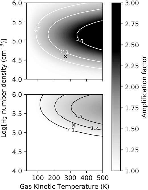
Contour and grey scale plot of the amplification factor (e−τ) for the J = 1 − 0 transition (upper panel) and the J = 2 − 1 transition (lower panel) in the |$\mathrm{n_{H_2}}$|−Tk plane when only collisions are included and with no beaming.
In equations (8) and (9), nℓ(r) is the radial dependent CS number density, Z(r) the partition function, |$\Delta \upsilon (r)$| the radial dependent velocity dispersion of the absorbing gas, XCS the CS abundance, and Eℓ, 0 = Eℓ − E0, with E0 the ground-state energy.
The radial dependence of the velocity dispersion was related to the kinetic temperature according to |$\Delta \upsilon (r) = 8.0\, \mathrm{km\, s^{-1}} (\mathrm{T_k}(r)/700\, \mathrm{K})^{0.31}$| which gives |$\Delta \upsilon \sim 3.0\, \mathrm{km\, s^{-1}}$| at 0.1 pc and beyond which it stayed constant at |$3.0\, \mathrm{km\, s^{-1}}$|. The velocity dispersion of 8.0 |$\mathrm{km\, s^{-1}}$| at 700 K follows from the work Barr et al. (2018). For the radial dependence of the CS fractional abundance, the result by Bruderer, Doty & Benz (2009) (see their Fig. 6) was modified to account for a higher CS fractional abundance as was argued earlier. The fractional abundance was therefore set at 2 × 10⁻⁵ at the position of the J = 2 − 1 maser and to decrease as a power law to 1.0 × 10⁻⁷ at 2 × 1016 cm. For r > 2 × 1016 cm, the fractional abundance was set at 5 × 10⁻⁹.
Using these radial dependencies in equations (8) and (9) and integrating up to rmax = 1 parsec gives τ = 0.6 for the J = 1 − 0 maser and τ = 1.4 for the J = 2 − 1 maser. The difference in optical depth between the two transitions is mainly due to the smaller radial position of the J = 2 − 1 maser and therefore also the increased density. It is also worth noting that ∼60 per cent of the optical depth for the J = 2 − 1 maser originates inside the hot core region while for the J = 1 − 0 maser ∼77 per cent of the optical depth is due to the cold gas outside the hot core. Since the radial dependencies used the calculation may not reflect the real situation for W51 e2e and does not consider any clumpiness, these values should only be used as a rough estimate. In spite of the uncertainties, these results suggest that attenuation of the J = 1 − 0 and J = 2 − 1 masers might be non-negligible. The implication is that such attenuation may result in completely obscuring the masers and be a contributing factor to the rarity of these masers. For W51 e2e, the implication is that the detection of the masers might be due to a ‘hole’ in the surrounding molecular material as suggested by Ginsburg & Goddi (2019).
5 CONCLUSIONS
We solved the rate equations for the first 31 rotational states of CS in the ground vibrational state and considered the effect of collisions, radiation and beaming on the level populations to determine the conditions under which the J = 1 − 0, J = 2 − 1, and J = 3 − 2 transitions are inverted. The main result from this study is that the three transitions can be inverted with collisions as the only excitation mechanism. To reproduce the brightness temperatures of the J = 1 − 0 and J = 2 − 1 masers in W51 e2e, a beaming factor of the form (2τ + 1)−2 is required. Brightness temperatures between 5000 and 9000 K can be obtained for the J = 1 − 0 maser for H2 densities between 105 and 104 cm−3 and corresponding kinetic temperatures from about 250 to 500 K, respectively. For the J = 2 − 1 maser, similar brightness temperatures occur for H2 densities between 105 and 105.5 cm−3 and corresponding kinetic temperatures between about 250 and 500 K. A significant further result is that the two masers never have their maximum gain at the same CS specific column density.
No clear conclusion can be made at this time on why the CS masers are rare. It is, however, remarkable that the CS abundance derived by Highberger et al. (2000) for the |$\upsilon \!=\!1$|, J = 3 − 2 maser in IRC+10216 is very similar to what is inferred from the model calculations for the |$\upsilon \!=\!0$|, J = 1 − 0, and J = 2 − 1 masers. Since the CS abundance is IRC+10216 is abnormally high, it might also be the case for W51 e2e and be the reason why CS masers are rare. On the other hand, Barr et al. (2018) have shown that a high CS abundance is also present in AFGL 2591 implying that W51 e2e might not be unique in this regard. It will be useful to also try to determine the CS abundance observationally in W51 e2e in the region where the two masers operate. We also conclude that attenuation of the maser emission inside and outside of the hot core might be a contributing factor for the non-detection of the masers.
The detection of the CS(J = 1 − 0) and CS(J = 2 − 1) masers in W51 e2e raises other questions as well. For example, since the pumping of the 6.7-GHz methanol masers require the kinetic temperature to be less than the dust temperature (∼100 K) (Sobolev et al. 1997; Cragg et al. 2002), what is the relation between the CS J = 1 − 0 and the 6.7-GHz methanol masers that are in projection rather close to each other? Furthermore, if the 6.7-GHz methanol masers indeed require maser path-lengths of about 1017 cm (6700 au), what physical structure are they associated with? A second question is that if a high CS abundance is not the reason for the rarity of the CS masers, what else can be the reason? If the rarity of the CS masers in high-mass star-forming regions is indeed due to a required high CS abundance, why is it that this requirement is met in W51 e2e and not in the other high-mass young stellar objects in W51?
DATA AVAILABILITY
No new data were generated or analysed in support of this research. The code used to obtain the numerical results will be shared on reasonable request to the corresponding author.
