


ABSTRACT
Subdwarf B stars are core-helium-burning stars located on the extreme horizontal branch (EHB). Extensive mass loss on the red giant branch is necessary to form them. It has been proposed that substellar companions could lead to the required mass loss when they are engulfed in the envelope of the red giant star. J08205+0008 was the first example of a hot subdwarf star with a close, substellar companion candidate to be found. Here, we perform an in-depth re-analysis of this important system with much higher quality data allowing additional analysis methods. From the higher resolution spectra obtained with ESO-VLT/XSHOOTER, we derive the chemical abundances of the hot subdwarf as well as its rotational velocity. Using the Gaia parallax and a fit to the spectral energy distribution in the secondary eclipse, tight constraints to the radius of the hot subdwarf are derived. From a long-term photometric campaign, we detected a significant period decrease of |$-3.2(8)\times 10^{-12} \, \rm dd^{-1}$|. This can be explained by the non-synchronized hot subdwarf star being spun up by tidal interactions forcing it to become synchronized. From the rate of period decrease we could derive the synchronization time-scale to be 4 Myr, much smaller than the lifetime on EHB. By combining all different methods, we could constrain the hot subdwarf to a mass of |$0.39\!-\!0.50\, \rm M_\odot$| and a radius of |$R_{\rm sdB}=0.194\pm 0.008\, \rm R_\odot$|, and the companion to |$0.061\!-\!0.071\rm \, M_\odot$| with a radius of |$R_{\rm comp}=0.092 \pm 0.005\, \rm R_\odot$|, below the hydrogen-burning limit. We therefore confirm that the companion is most likely a massive brown dwarf.
1 INTRODUCTION
Subluminous B stars (subdwarf B stars or sdBs) are stars with thin hydrogen envelopes, currently undergoing helium-core burning, which are found on the extreme horizontal branch (EHB). Their masses were determined to be around 0.47 M⊙ (Heber 2009, 2016). About half of the known single-lined sdB stars are found to be members of short-period binaries (P ≲ 30 d, most even with P ≲ 10 d, Maxted et al. 2001; Napiwotzki et al. 2004a; Kupfer et al. 2015). A large mass loss on the red giant branch (RGB) is required to form these stars, which can be caused by mass transfer to the companion, either via stable Roche lobe overflow or the formation and eventual ejection of a common envelope (Han et al. 2002, 2003). For the existence of apparently single sdB stars binary evolution might play an important role as well, as such stars could be remnants of helium white dwarf (WD) mergers (Webbink 1984; Iben & Tutukov 1984) or from engulfing a substellar object, which might get destroyed in the process (Soker 1998; Nelemans & Tauris 1998).
Eclipsing sdB+dM binaries (HW Vir systems) having short orbital periods (|$0.05\!-\!1\, {\rm d}$|) and low companion masses between 0.06 and 0.2 M⊙ (see Schaffenroth et al. 2018, 2019, for a summary of all known HW Vir systems) have been known for decades (Menzies & Marang 1986) and illustrate that objects close to the nuclear-burning limit of ∼0.070–0.076 M⊙ for an object of solar metallicity and up to |$0.09\, \rm M_{\rm \odot }$| for metal-poor objects (see Dieterich et al. 2014, for a review) can eject a common envelope and lead to the formation of an sdB. The light traveltime technique was used to detect substellar companion candidates to sdB stars (e.g. Beuermann et al. 2012; Kilkenny & Koen 2012, and references therein). However, in these systems the substellar companions have wide orbits and therefore cannot have influenced the evolution of the host star.
The short-period eclipsing HW Vir type binary SDSS J082053.53+000843.4, hereafter J08205+0008, was discovered as part of the MUCHFUSS project (Geier et al. 2011a, b). Geier et al. (2011c) derived an orbital solution based on time-resolved medium resolution spectra from Sloan Digital Sky Survey (SDSS) (Abazajian et al. 2009) and ESO-NTT/EFOSC2. The best-fitting orbital period was |$P_{\rm orb}=P=0.096\pm 0.001\, {\rm d}$| and the radial velocity (RV) semi-amplitude |$K=47.4\pm 1.9\, {\rm km\, s^{-1}}$| of the sdB. An analysis of a light curve taken with Merope on the Mercator telescope allowed them to constrain the inclination of the system to 85.8° ± 0.16.
The analysis resulted in two different possible solutions for the fundamental parameters of the sdB and the companion. As the sdB sits on the EHB the most likely solution is a core-He-burning object with a mass close to the canonical mass for the He flash of |$0.47 \, \rm M_\odot$|. Population synthesis models (Han et al. 2002, 2003) predict a mass range of |$M_{\rm sdB}=0.37\!-\!0.48\, \rm M_\odot$|, which is confirmed by asteroseismological measurements (Fontaine et al. 2012). A more massive (|$2\!-\!3\, \rm M_\odot$|) progenitor star would ignite the He core under non-degenerate conditions and lower masses down to |$0.3\, \rm M_\odot$| are possible. Due to the shorter lifetime of the progenitors such lower mass hot subdwarfs would also be younger. Higher masses for the sdB were ruled out as contemporary theory did not predict that. By a combined analysis of the spectrum and the light curve, the companion was derived to have a mass of |$0.068\pm 0.003\, \rm M_\odot$|. However, the derived companion radius for this solution was significantly larger than predicted by theory.
The second solution that was consistent with the atmospheric parameters was a post-RGB star with an even lower mass of only |$0.25\, \rm M_\odot$|. Such an object can be formed whenever the evolution of the star on the RGB is interrupted due to the ejection of a common envelope before the stellar core mass reaches the mass, which is required for helium ignition. Those post-RGB stars, also called pre-helium WDs, cross the EHB and evolve directly to WDs. In this case, the companion was determined to have a mass of |$0.045\pm 0.003\, \rm M_\odot$| and the radius was perfectly consistent with theoretical predictions.
The discovery of J08205+0008 was followed by the discovery of two more eclipsing systems with brown dwarf (BD) companions, J162256+473051 (Schaffenroth et al. 2014a) and V2008−1753 (Schaffenroth et al. 2015), both with periods of less than 2 h. Two non-eclipsing systems were also discovered by Schaffenroth et al. (2014b), and a subsequent analysis of a larger population of 26 candidate binary systems by Schaffenroth et al. (2018) suggests that the fraction of sdB stars with close substellar companions is as high as 3 per cent, much higher than the 0.5 ± 0.3 per cent that is estimated for BD companions to WDs (e.g. Steele et al. 2011). Seven of the nine known WD–BD systems have primary masses within the mass range for an He-core-burning hot subdwarf and might therefore have evolved through this phase before.
In this paper, we present new phase-resolved spectra of J08205+0008 obtained with ESO-VLT/UVES and XSHOOTER and high cadence light curves with ESO-NTT/ULTRACAM (ULTRAfast CAMera). Combining these data sets, we have refined the RV solution and light-curve fit. We performed an in-depth analysis of the sdB atmosphere and a fit of the spectral energy distribution (SED) using the ULTRACAM secondary eclipse measurements to better constrain the radius and mass of the sdB primary and the companion. We also present our photometric campaign using the South African Astronomical Observatory (SAAO)/1-m telescope and Bonn University Simultaneous CAmera (BUSCA) mounted at the Calar Alto/2.2m telescope which has been underway for more than 10 yr now, and which has allowed us to derive variations of the orbital period.
2 SPECTROSCOPIC AND PHOTOMETRIC DATA
2.1 UVES spectroscopy
We obtained time-resolved, high-resolution (|$R\simeq 40\, 000$|) spectroscopy of J08205+0008 with ESO-VLT/UVES (Dekker et al. 2000) on the night of 2011 April 05 as part of program 087.D-0185(A). In total 33 single spectra with exposure times of |$300\, {\rm s}$| were taken consecutively to cover the whole orbit of the binary. We used the 1 arcsec slit in seeing of ∼1 arcsec and airmass ranging from 1.1. to 1.5. The spectra were taken using cross dispersers CD nos 2 and 3 on the blue and red chips, respectively, to cover a wavelength range from 3300 to 6600 Å with two small gaps (≃100 Å) at 4600 and 5600 Å.
The data reduction was done with the UVES reduction pipeline in the midas package (Banse et al. 1983). In order to ensure an accurate normalization of the spectra, two spectra of the DQ-type white dwarf WD 0806−661 were also taken (Subasavage et al. 2009). Since the optical spectrum of this carbon-rich WD is featureless, we divided our data by the co-added and smoothed spectrum of this star.
The individual spectra of J08205+0008 were then RV corrected using the derived RV of the individual spectra as described in Section 3.6 and co-added for the atmospheric analysis. In this way, we increased the signal-to-noise ratio to S/N ∼ 90, which was essential for the subsequent quantitative analysis.
2.2 XSHOOTER spectroscopy
We obtained time resolved spectra of J08205+0008 with ESO-VLT/XSHOOTER (Vernet et al. 2011) as part of programme 098.C-0754(A). The data were observed on the night of 2017 February 17 with 300 s exposure times in nod mode and in seeing of 0.5–0.8 arcsec. We obtained 24 spectra covering the whole orbital phase (see Fig. B1) in each of the UVB (R ∼ 5400), VIS (R ∼ 8900), and NIR (R ∼ 5600) arms with the 0.9–1.0 arcsec slits. The spectra were reduced using the ESO reflex package (Freudling et al. 2013) and the specific XSHOOTER routines in nod mode for the NIR arm, and in stare mode for the UVB and VIS arms.
To correct the astronomical observations for atmospheric absorption features in the VIS and NIR arms, we did not require any observations of telluric standard stars, as we used the molecfit software, which is based on fitting synthetic transmission spectra calculated by a radiative transfer code to the astronomical data (Smette et al. 2015; Kausch et al. 2015). The parameter set-up (fitted molecules, relative molecular column densities, degree of polynomial for the continuum fit, etc.) for the telluric absorption correction evaluation of the NIR-arm spectra were used according to table 3 of Kausch et al. (2015). Unfortunately, the NIR arm spectra could not be used after the telluric corrections since the S/N ratio and the fluxes are too low. Fig. A1 shows an example comparison between the original and the telluric absorption corrected XSHOOTER VIS arm spectra. The quality of the telluric correction is sufficient to allow us to make use of the hydrogen Paschen series for the quantitative spectral analysis.
Accurate RV measurements for the single XSHOOTER spectra were performed within the analysis program spas (Spectral Analysis Software) (Hirsch 2009), whereby selected sharp metal lines listed in Table D1 were used. We used a combination of Lorentzian, Gaussian, and straight line (in order to model the slope of the continuum) function to fit the line profiles of the selected absorption lines. After having corrected all single spectra by the averaged RVs, a co-added spectrum was created in order to achieve S/N ∼ 460/260 in the UVB and VIS channels, respectively.
The co-added spectrum then was normalized also within spas. Numerous anchor points were set where the stellar continuum to be normalized was assumed. In this way, the continuum was approximated by a spline function. To obtain the normalized spectrum, the original spectrum was divided by the spline.
2.3 ULTRACAM photometry
Light curves in the SDSS u′g′r′ filters were obtained simultaneously using the ULTRACAM instrument (Dhillon et al. 2007) on the 3.5-m-ESO-NTT at La Silla. The photometry was taken on the night of 2017 March 19 with airmass 1.15–1.28 as part of programme 098.D-679 (PI: Schaffenroth). The data were taken in full frame mode with 1 × 1 binning and the slow readout speed with exposure times of 5.75 s resulting in 1755 frames obtained over the full orbit of the system. The dead-time between each exposure was only 25 ms. We reduced the data using the HiperCam pipeline (http://deneb.astro.warwick.ac.uk/phsaap/hipercam/docs/html). The flux of the sources was determined using aperture photometry with an aperture scaled variably according to the full width at half-maximum. The flux relative to a comparison star within the field of view (08:20:51.941 +00:08:21.64) was determined to account for any variations in observing conditions. This reference star has SDSS magnitudes of u′=15.014 ± 0.004, g′=13.868 ± 0.003, and r′=13.552 ± 0.003 which were used to provide an absolute calibration for the light curve.
2.4 SAAO photometry
All the photometry was obtained on the 1-m (Elizabeth) telescope at the Sutherland site of the SAAO. Nearly all observations were made with the STE3 CCD, except for the last two (Table G1), which were made with the STE4 camera. The two cameras are very similar with the only difference being the pixel size as the STE3 is 512 × 512 pixels in size and the STE4 is 1024 × 1024. We used a 2 × 2 pre-binned mode for each CCD resulting in a read-out time of around 5 and 20 s, respectively, so that with typical exposure times around 10–12s, the time resolution of STE4 is only about half as good as STE3. Data reduction and eclipse analysis were carried out as outlined in Kilkenny (2011); in the case of J08205+008, there are several useful comparison stars, even in the STE3 field, and – given that efforts were made to observe eclipses near the meridian – usually there were no obvious ‘drifts’ caused by differential extinction effects. In the few cases where such trends were seen, these were removed with a linear fit to the data from just before ingress and just after egress. The stability of the procedures (and the SAAO time system over a long time base) is demonstrated by the constant-period system AA Dor (fig. 1 of Kilkenny 2014) and by the intercomparisons in fig. 8 of Baran et al. (2018), for example.
2.5 BUSCA photometry
Photometric follow-up data were also taken with the BUSCA (see Reif et al. 1999), which is mounted to the 2.2-m telescope located at the Calar Alto Observatory in Spain. This instrument observes in four bands simultaneously giving a very accurate eclipse measurement and good estimate of the errors. The four different bands we used in our observation are given solely by the intrinsic transmission curve given by the beam splitters (UB, BB, RB, IB, http://www.caha.es/CAHA/Instruments/BUSCA/bands.txt) and the efficiency of the CCDs, as no filters where used to ensure that all the visible light is used most efficiently.
The data were taken during one run on 2011 February 25 and March 1. We used an exposure time of 30 s. Small windows were defined around the target and four comparison stars to decrease the read-out time from 2 min to 15 s. As comparison stars we used stars with similar magnitudes (Δm < 2 mag) in all SDSS bands from u to z, which have been pre-selected using the SDSS DR 9 skyserver (http://skyserver.sdss.org/dr9/en/). The data were reduced using iraf;1 a standard CCD reduction was performed using the iraf tools for bias- and flat-field corrections. Then, the light curves of the target and the comparison stars were extracted using the aperture photometry package of daophot. The final light was constructed by dividing the light curve of the target by the light curves of the comparison stars.
3 ANALYSIS
3.1 The hybrid LTE/NLTE approach and spectroscopic analysis
Both the co-added UVES and XSHOOTER (UVB and VIS arm) spectra were analysed using the same hybrid local thermodynamic equilibrium (LTE)/non-LTE (NLTE) model atmospheric approach. This approach has been successfully used to analyse B-type stars (see, for instance, Przybilla, Nieva & Edelmann 2006a; Przybilla et al. 2006b; Nieva & Przybilla 2007, 2008; Przybilla, Nieva & Butler 2011) and is based on the three generic codes atlas12 (Kurucz 1996), detail, and surface (Giddings 1981; Butler & Giddings 1985, extended and updated).
Based on the mean metallicity for hot subdwarf B stars according to Naslim et al. (2013), metal-rich and line-blanketed, plane-parallel and chemically homogeneous model atmospheres in hydrostatic and radiative equilibrium were computed in LTE within atlas12. Occupation number densities in NLTE for hydrogen, helium, and for selected metals (see Table B1) were computed with detail by solving the coupled radiative transfer and statistical equilibrium equations. The emergent flux spectrum was synthesized afterwards within surface, making use of realistic line-broadening data. Recent improvements to all three codes (see Irrgang et al. 2018, for details) with regard to NLTE effects on the atmospheric structure as well as the implementation of the occupation probability formalism (Hubeny, Hummer & Lanz 1994) for H i and He ii and new Stark broadening tables for H (Tremblay & Bergeron 2009) and He i (Beauchamp, Wesemael & Bergeron 1997) are considered as well. For applications of these models to sdB stars, see Schneider et al. (2018).
We included spectral lines of H and |$\mathrm{He\,{\small I}}$|, and in addition, various metals in order to precisely measure the projected rotational velocity (vsin i), RV (vrad), and chemical abundances of J08205+0008. The calculation of the individual model spectra is presented in detail in Irrgang et al. (2014). In Table B2, the covered effective temperatures, surface gravities, helium, and metal abundances for the hybrid LTE/NLTE model grid used are listed.
The quantitative spectral analysis followed the methodology outlined in detail in Irrgang et al. (2014), that is, the entire useful spectrum and all 15 free parameters (Teff, log g, vrad, vsin i, |$\log {n(\text{He})}:=\log {\left[\frac{\text{N(He)}}{\text{N(all elements)}}\right]}$|, plus abundances of all metals listed in Table B1) were simultaneously fitted using standard χ2 minimization techniques. Macroturbulence ζ and microturbulence ξ were fixed to zero because there is no indication for additional line-broadening due to these effects in sdB stars (see, for instance, Geier & Heber 2012; Schneider et al. 2018).
3.2 Effective temperature, surface gravity, helium content, and metal abundances
The excellent match of the global best-fitting model spectrum to the observed one is demonstrated in Fig. 1 for selected spectral ranges in the co-added XSHOOTER spectrum of J08205+0008 (UVB + VIS arm).
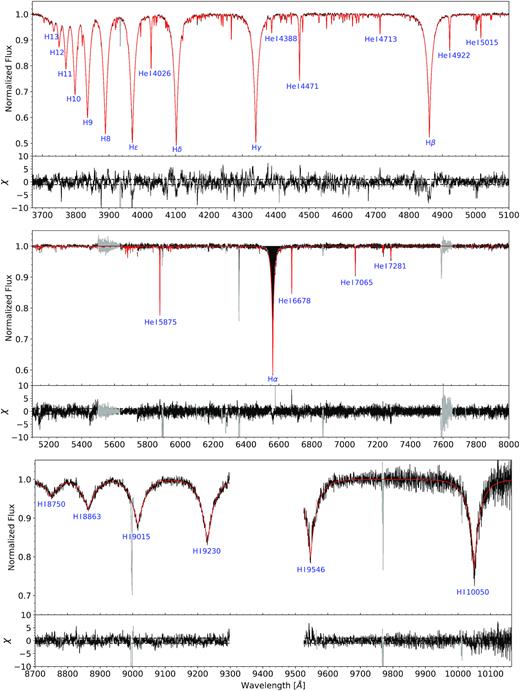
Comparison between observation (solid black line) and global best fit (solid red line) for selected spectral ranges in the co-added XSHOOTER spectrum of J08205+0008. Prominent hydrogen and |$\mathrm{He\,{\small I}}$| lines are marked by blue labels and the residuals for each spectral range are shown in the bottom panels, whereby the dashed horizontal lines mark mark deviations in terms of ±1σ, that is, values of χ = ±1 (0.2 per cent in UVB and 0.4 per cent in VIS, respectively). Additional absorption lines are caused by metals (see Fig. 4). Spectral regions, which have been excluded from the fit, are marked in grey (observation) and dark red (model), respectively. Since the range between H i 9230 Å and H i 9546 Å strongly suffers from telluric lines (even after the telluric correction with molecfit), it is excluded from the figure.
The wide spectral range covered by the XSHOOTER spectra allowed, besides the typical hydrogen Balmer series and prominent |$\mathrm{He\,{\small I}}$| lines in the optical, Paschen lines to be included in the fit, which provides additional information that previously could not be used in sdB spectral analysis, but provides important consistency checks.
In the framework of our spectral analysis, we also tested for variations of the atmospheric parameters over the orbital phase as seen in other reflection effect systems (e.g. Heber et al. 2004; Schaffenroth et al. 2013). As expected, due to the relatively weak reflection effect of less than 5 per cent, the variations were within the total uncertainties given in the following and can therefore be neglected (see also Fig. B1 for details).
The resulting effective temperatures, surface gravities, and helium abundances derived from XSHOOTER and UVES are listed in Table 3. The results include 1σ statistical errors and systematic uncertainties according to the detailed study of Lisker et al. (2005), which has been conducted in the framework of the ESO Supernova Ia Progenitor Survey. For stars with two exposures or more, Lisker et al. (2005) determined a systematic uncertainty of ±374 K for Teff, ± 0.049 dex for log (g), and ± 0.044 dex for log n(He) (see table 2 in Lisker et al. 2005 for details).
Fig. 2 shows the Teff–log (g) diagram, where we compare the UVES and XSHOOTER results to predictions of evolutionary models for the horizontal branch for a canonical mass sdB with different envelope masses from Dorman et al. (1993), as well as evolutionary tracks assuming solar metallicity and masses of 0.50 and 0.55 M⊙ (Han et al. 2002). With |$T_{\text{eff}}=26\, 000\pm 400$| K and log (g) = 5.54 ± 0.05 (XSHOOTER, statistical and systematic errors) and |$T_{\text{eff}}=25\, 600\pm 400$| K and log (g) = 5.51 ± 0.05 (UVES, statistical and systematic errors), J08205+0008 lies within the EHB, as expected. Our final result (|$T_{\text{eff}}=25\, 800\pm 290$| K, log (g) = 5.52 ± 0.04), the weighted average of the XSHOOTER and UVES parameters, is also in good agreement with the LTE results of Geier et al. (2011c), which are |$T_{\text{eff}}=26\, 700\pm 1000$| K and log (g) = 5.48 ± 0.10, respectively.
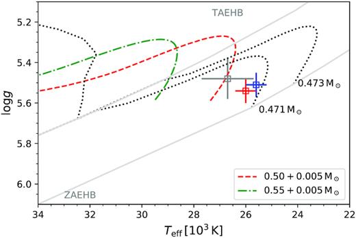
Teff–log (g) diagram for J08205+0008. While the blue square represents the UVES solution, the red square results from XSHOOTER. The grey square marks the LTE solution of Geier et al. (2011c). The ZAEHB and terminal-age horizontal branch (TAEHB) for a canonical mass sdB are shown in grey as well as evolutionary tracks for a canonical mass sdB with different envelope masses from Dorman, Rood & O’Connell (1993) with black dotted lines. Additionally, we show evolutionary tracks with solar metallicity for different sdB masses with hydrogen layers of |$0.005\rm \, M_\odot$|, according to Han et al. (2002) to show the mass dependence of the EHB. The error bars include 1σ statistical and systematic uncertainties as presented in the text (see Section 3.2 for details).
The determined helium content of J08205+0008 is log n(He) = −2.06 ± 0.05 (XSHOOTER, statistical and systematic errors) and log n(He) = −2.07 ± 0.05 (UVES, statistical and systematic errors), hence clearly subsolar (see Asplund et al. 2009 for details). The final helium abundance (log n(He) = −2.07 ± 0.04), the weighted average of XSHOOTER and UVES, therefore is comparable with Geier et al. (2011c), who measured log n(He) = −2.00 ± 0.07, and with the mean helium abundance for sdB stars from Naslim et al. (2013), which is log n(He) = −2.34 (see also Fig. 3).
![The chemical abundance pattern of J08205+0008 (red: XSHOOTER and blue: UVES) relative to solar abundances of Asplund et al. (2009), represented by the black horizontal line. The orange solid line represents the mean abundances for hot subdwarf B stars according to Naslim et al. (2013) used as the metallicity for our quantitative spectral analysis. Upper limits are marked with downward arrows and $\left[\frac{{N}({X})}{{N}(\text{total})}\right]:=\log _{10}{ \left\lbrace \frac{{N}({X})}{{N}(\text{total})}\right\rbrace }-\log _{10}{\left\lbrace \frac{{N}({X(\mathrm{ solar})})}{{N}(\text{total})}\right\rbrace }$.](https://oup.silverchair-cdn.com/oup/backfile/Content_public/Journal/mnras/501/3/10.1093_mnras_staa3661/1/m_staa3661fig3.jpeg?Expires=1750006254&Signature=xHerUsDuGH0-p9Wh9vf4RCqYJy9~Vc8sfSCZduLSJ0ld9CZlg3nTW9Xq7dSujkrN8QqowcqhkGmTjGew~pWkgsJ4k3YNolCXhpl7iZMpRAWBaervqVeGwooDXSC2OZRY1PpWX8t-~2buXxZh33TiuTaR4fPdSSz0XKr6lKIbVJeihEOVPy9UcxkhFqqx~WWiy9LXUewGIf2gNctdLd5TY-f3HiXuh~lbK7vUKlYXuiWdDXmo4038K2FoXVeh~Gk6ShSP79EzATuGL7rzJfLLte-hVdHYQP3VJMFoZmhx2-pXfKKSr9wudhoNb4z5lZBbUt1XqqDEOSeTRziRyRSI6A__&Key-Pair-Id=APKAIE5G5CRDK6RD3PGA)
The chemical abundance pattern of J08205+0008 (red: XSHOOTER and blue: UVES) relative to solar abundances of Asplund et al. (2009), represented by the black horizontal line. The orange solid line represents the mean abundances for hot subdwarf B stars according to Naslim et al. (2013) used as the metallicity for our quantitative spectral analysis. Upper limits are marked with downward arrows and |$\left[\frac{{N}({X})}{{N}(\text{total})}\right]:=\log _{10}{ \left\lbrace \frac{{N}({X})}{{N}(\text{total})}\right\rbrace }-\log _{10}{\left\lbrace \frac{{N}({X(\mathrm{ solar})})}{{N}(\text{total})}\right\rbrace }$|.
Moreover, it was possible to identify metals of various different ionization stages within the spectra (see Table D1 and Fig. 4) and to measure their abundances. Elements found in more than one ionization stage are oxygen (|$\mathrm{O\,{\small I/II}}$|), silicon (|$\mathrm{Si\,{\small II/III}}$|), and sulfur (|$\mathrm{S\,{\small II/III}}$|), whereas carbon (|$\mathrm{C\,{\small II}}$|), nitrogen (|$\mathrm{N\,{\small II}}$|), magnesium (|$\mathrm{Mg\,{\small II}}$|), aluminum (|$\mathrm{Al\,{\small III}}$|), argon (|$\mathrm{Ar\,{\small II}}$|), and iron (|$\mathrm{Fe\,{\small III}}$|) are only detected in a single stage. We used the model grid in Table B2 to measure the individual metal abundances in both the co-added XSHOOTER and the UVES spectrum. We were able to fit the metal lines belonging to different ionization stages of the same elements similarly well (see Fig. 4). The corresponding ionization equilibria additionally constrained the effective temperature.
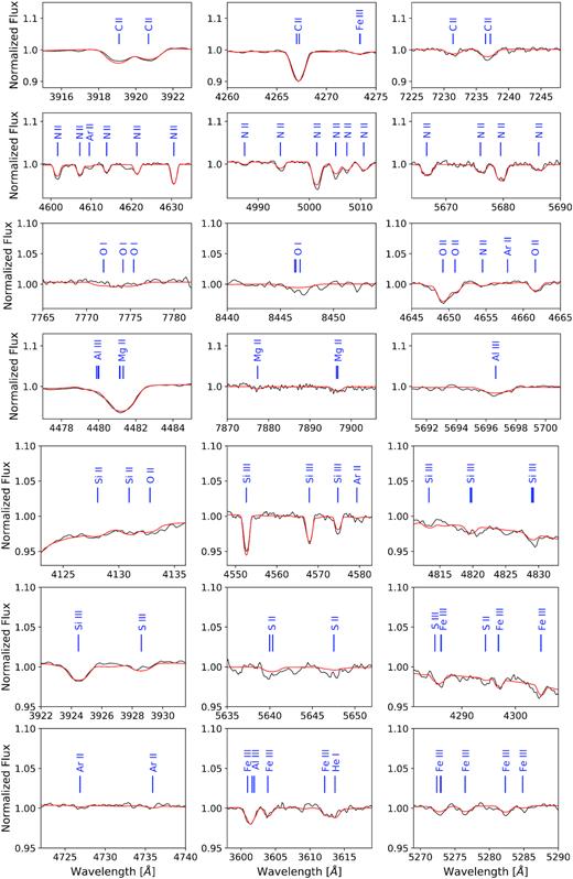
Selected metal lines in the co-added XSHOOTER spectrum of J08205+0008. The observed spectrum (solid black line) and the best fit (solid red line) are shown. Solid blue vertical lines mark the central wavelength positions and the ionization stages of the individual metal lines according to Table D1.
All metal abundances together with their total uncertainties are listed in Table 1. Systematic uncertainties were derived according to the methodology presented in detail in Irrgang et al. (2014) and cover the systematic uncertainties in effective temperature and surface gravity as described earlier.
Metal abundances of J08205+0008 derived from XSHOOTER and UVES.†
| Parameter | XSHOOTER | UVES |
|---|---|---|
| log n(C) | −4.38 ± 0.05 | |$-4.39^{+0.04}_{-0.03}$| |
| log n(N) | |$-4.00^{+0.03}_{-0.02}$| | −3.98 ± 0.03 |
| log n(O) | |$-4.01^{+0.05}_{-0.06}$| | |$-3.86^{+0.07}_{-0.06}$| |
| log n(Ne) | ≤−6.00 | ≤−6.00 |
| log n(Mg) | |$-4.98^{+0.05}_{-0.04}$| | −5.03 ± 0.05 |
| log n(Al) | −6.20 ± 0.03 | ≤−6.00 |
| log n(Si) | −5.13 ± 0.04 | |$-5.17^{+0.07}_{-0.08}$| |
| log n(S) | |$-5.31^{+0.11}_{-0.10}$| | |$-5.12^{+0.06}_{-0.08}$| |
| log n(Ar) | |$-5.54^{+0.15}_{-0.27}$| | |$-5.32^{+0.19}_{-0.23}$| |
| log n(Fe) | −4.39 ± 0.04 | |$-4.41^{+0.04}_{-0.05}$| |
Notes:†Including 1σ statistical and systematic errors.
|$\log {n({X})}:=\log {\left[\frac{{N(X)}}{{N(\mathrm{ all\,elements})}}\right]}$|
The results of XSHOOTER and UVES are in good agreement, except for the abundances of oxygen, sulfur, and argon, where differences of 0.15, 0.19, and 0.22 dex, respectively, are measured. However, on average these metals also have the largest uncertainties, in particular argon, such that the abundances nearly overlap if the corresponding uncertainties are taken into account. According to Fig. 3, J08205+0008 is underabundant in carbon and oxygen, but overabundant in nitrogen compared to solar (Asplund et al. 2009), showing the prominent CNO signature as a remnant of the star’s hydrogen core-burning through the CNO cycle. Aluminum and the alpha elements (neon, magnesium, silicon, and sulfur) are underabundant compared to solar. With the exception of neon, which is not present, the chemical abundance pattern of J08205+0008 generally follows the metallicity trend of hot subdwarf B stars (Naslim et al. 2013), even leading to a slight enrichment in argon and iron compared to solar. The latter may be explained by radiative levitation, which occurs in the context of atomic transport, that is, diffusion processes in the stellar atmosphere of hot subdwarf stars (Greenstein 1967; see Michaud, Alecian & Richer 2015 for a detailed review).
Due to the high resolution of the UVES (and XSHOOTER) spectra, we were also able to measure the projected rotational velocity of J08205+0008 from the broadening of the spectral lines, in particular from the sharp metal lines, to |$v\sin {i}=66.0\pm 0.1\, {\rm km\, s^{-1}}$| (UVES, 1σ statistical errors only) and |$v\sin {i}=65.8\pm 0.1\, {\rm km\, s^{-1}}$| (XSHOOTER, 1σ statistical errors only).
3.3 Search for chemical signatures of the companion
Although HW Vir type systems are known to be single-lined, traces of the irradiated and heated hemisphere of the cool companion have been found in some cases. Wood & Saffer (1999) discovered the Hα absorption component of the companion in the prototype system HW Vir (see also Edelmann 2008).
Metal lines in emission were found in the spectra of the hot sdOB star AA Dor by Vučković et al. (2016) moving in antiphase to the spectrum of the hot sdOB star indicating an origin near the surface of the companion. After the removal of the contribution of the hot subdwarf primary, which is dominating the spectrum, the residual spectra showed more than 100 shallow emission lines originating from the heated side of the secondary, which show their maximum intensity close to the phases around the secondary eclipse. They analysed the residual spectrum in order to model the irradiation of the low-mass companion by the hot subdwarf star. The emission lines of the heated side of the secondary star allowed them to determine the RV semi-amplitude of the centre of light. After the correction to the centre of mass of the secondary they could derive accurate masses of both components of the AA Dor system, which is consistent with a canonical sdB mass of |$0.46\, \rm M_\odot$| and a companion of |$0.079\pm 0.002\rm \, M_\odot$| very close to the hydrogen-burning limit. They also computed a first generation atmosphere model of the low mass secondary including irradiation effects.
J08205+0008 is significantly fainter and cooler than AA Dor but with a much shorter period. We searched the XSHOOTER spectra for signs of the low-mass companion of J08205+0008. This was done by subtracting the spectrum in the secondary minimum where the companion is eclipsed from the spectra before and after the secondary eclipse where most of the heated atmosphere of the companion is visible. However, no emission or absorption lines from the companion were detected (see Figs E1 and E2). Also, in the XSHOOTER NIR arm spectra, no emission lines could be found.
3.4 Photometry: angular diameter and interstellar reddening
The angular diameter of a star is an important quantity, because it allows the stellar radius to be determined, if the distance is known, for example, from trigonometric parallax. The angular diameter can be determined by comparing observed photometric magnitudes to those calculated from model atmospheres for the stellar surface. Because of contamination by the reflection effect the apparent magnitudes of the hot subdwarf can be measured only during the secondary eclipse, where the companion is completely eclipsed by the larger subdwarf. We performed a least-squares fit to the flat bottom of the secondary eclipse in the ULTRACAM light curves to determine the apparent magnitudes and derived u′ = 14.926 ± 0.009 mag, g′ = 15.025 ± 0.004 mag, and r′ = 15.450 ± 0.011 mag (1σ statistical errors).
Because the star lies at low Galactic latitude (b = 19°) interstellar reddening is expected to be significant. Therefore, both the angular diameter and the interstellar colour excess have to be determined simultaneously. We used the reddening law of Fitzpatrick et al. (2019) and matched a synthetic flux distribution calculated from the same grid of model atmospheres that where also used in the quantitative spectral analysis (see Section 3.1) to the observed magnitudes as described in Heber, Irrgang & Schaffenroth (2018). The χ2 based fitting routine uses two free parameters: the angular diameter θ, which shifts the fluxes up and down according to f(λ) = θ2F(λ)/4, where f(λ) is the observed flux at the detector position and F(λ) is the synthetic model flux at the stellar surface, and the colour excess.2 The final atmospheric parameters and their respective uncertainties derived from the quantitative spectral analysis (see Section 3.2) result in an angular diameter of |$\theta = 6.22\, (\pm 0.15) \times 10^{-12}\, \rm rad$| and an interstellar reddening of E(B − V) = 0.041 ± 0.013 mag. The latter is consistent with values from reddening maps of Schlegel, Finkbeiner & Davis (1998) and Schlafly & Finkbeiner (2011): 0.039 and 0.034 mag, respectively.
In addition, ample photometric measurements of J08205+0008 are available in different filter systems, covering the spectral range all the way from the ultraviolet (GALEX) through the optical (e.g. SDSS) to the infrared (2MASS, UKIDDS, and WISE, see Fig. 5). However, those measurements are mostly averages of observations taken at multiple epochs or single epoch measurements at unknown orbital phase. Therefore, those measurements do not allow us to determine the angular diameter of the sdB because of the contamination by light from the heated hemisphere of the companion. However, an average SED of the system can be derived. This allows us to redetermine the interstellar reddening and to search for an infrared excess caused by light from the cool companion.
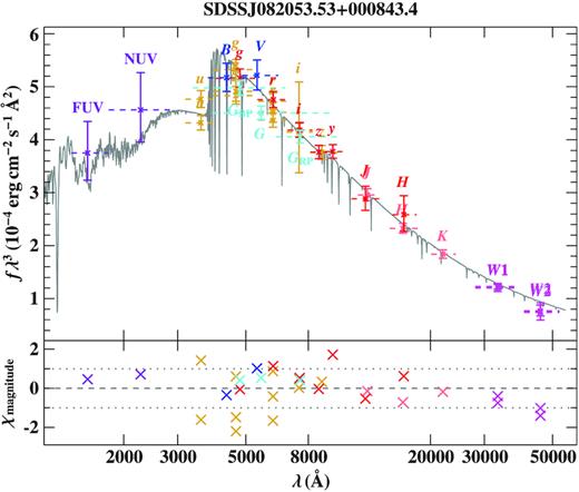
Comparison of synthetic and observed photometry: top panel: SED: filter-averaged fluxes converted from observed magnitudes are shown in different colours. The respective full width at tenth maximum are shown as dashed horizontal lines. The best-fitting model, degraded to a spectral resolution of 6 Å is plotted in grey. In order to reduce the steep SED slope the flux is multiplied by the wavelength cubed. Bottom panel: difference between synthetic and observed magnitudes divided by the corresponding uncertainties (residual χ). The following colour code is used for the different photometric systems: GALEX (violet, Bianchi, Shiao & Thilker 2017), SDSS (golden, Alam et al. 2015), Pan-STARRS1 (dark red, Flewelling et al. 2020), Johnson (blue, Henden et al. 2015), Gaia (cyan, Evans et al. 2018, with corrections and calibrations from Maíz Apellániz & Weiler 2018), 2MASS (red, Cutri et al. 2003), UKIDSS (pink, Lawrence et al. 2007), and WISE (magenta, Cutri et al. 2014; Schlafly, Meisner & Green 2019).
The same fitting technique is used in the analysis of the SED as described above for the analysis of the ULTRACAM magnitudes. Besides the sdB grid, a grid of synthetic spectra of cool stars (|$2300\, {\rm K} \le T_{\rm eff} \le 15 000\, \rm K$|, Husser et al. 2013) is used. In addition to the angular diameter and reddening parameter, the temperature of the cool companion as well as the surface ratio are free parameters in the fit. The fit results in E(B − V) = 0.040 ± 0.010 mag, which is fully consistent with the one derived from the ULTRACAM photometry as well as with the reddening map. The apparent angular diameter is larger than that from ULTRACAM photometry by 2.8 per cent, which is caused by the contamination by light from the companion’s heated hemisphere. The effective temperature of the companion is unconstrained and the best match is achieved for the surface ratio of zero, which means there is no signature from the cool companion. In a final step we allow the effective temperature of the sdB to vary and determine it along with the angular diameter and the interstellar reddening, which results in Teff= 26900|$^{+1400}_{-1500}$| K in agreement with the spectroscopic result (see Fig. 5 for the comparison of synthetic and observed photometry).
3.5 Stellar radius, mass, and luminosity
Since Gaia data release 2 (DR2; Gaia Collaboration 2018), trigonometric parallaxes are available for a large sample of hot subdwarf stars, including J08205+0008 for which 10 per cent precision has been reached. We corrected for the Gaia DR2 parallax zero-point offset of −0.029 mas (Lindegren et al. 2018).
The respective uncertainties of the stellar parameters are derived by Monte Carlo error propagation. The uncertainties are dominated by the error of the parallax measurement. Results are summarized in Table 3. Using the gravity and effective temperature derived by the spectroscopic analysis, the mass for the sdB is |$M= 0.48^{+0.12}_{-0.09}$| M⊙ and its luminosity is |$L=16^{+3.6}_{-2.8}$| L⊙ in agreement with canonical models for EHB stars (see fig. 13 of Dorman et al. 1993). The radius of the sdB is calculated by the angular diameter and the parallax to |$R = 0.200^{+0.021}_{-0.018}$| R⊙.
3.6 Radial velocity curve and orbital parameters
The RVs of the individual XSHOOTER spectra were measured by fitting all spectral features simultaneously to synthetic models as described in Section 3.1.
Due to lower S/N of the individual UVES spectra, which were observed in poor conditions, only the most prominent features in the spectra are suitable for measuring the Doppler shifts. After excluding very poor quality spectra, RVs of the remaining 28 spectra were measured using the fitsb2 routine (Napiwotzki et al. 2004b) by fitting a set of different mathematical functions to the hydrogen Balmer lines as well as He i lines. The continuum is fitted by a polynomial, and the line wings and line core by a Lorentzian and a Gaussian function, respectively. The barycentrically corrected RVs together with formal 1σ errors are summarized in Table F1.
The orbital parameters T0, period P, system velocity γ, and RV semi-amplitude K as well as their uncertainties were derived with the same method described in Geier et al. (2011a). To estimate the contribution of systematic effects to the total error budget additional to the statistic errors determined by the fitsb2 routine, we normalized the χ2 of the most probable solution by adding systematic errors to each data point enorm until the reduced χ2 reached ≃1.0.
Combining the UVES and XSHOOTER RVs, we derived |$T_{0}=57801.54954\pm 0.00024\, {\rm d}$|, |$P=0.096241\pm 0.000003\, {\rm d}$|, K = 47.9 ± 0.4 km s−1, and the system velocity γ = 26.5 ± 0.4 km s−1. No significant systematic shift was detected between the two data sets and the systematic error added in quadrature was therefore very small enorm = 2.0 km s−1. The gravitational redshift is significant at |$1.6_{+0.05}^{-0.02}$| km s−1 and might be important if the orbit of the companion could be measured by future high-resolution measurements (see e.g. Vos et al. 2013).
To improve the accuracy of the orbital parameters even more we then tried to combine them with the RV data set from Geier et al. (2011c), medium-resolution spectra taken with ESO-NTT/EFOSC2 and SDSS. A significant, but constant systematic shift of +17.4 km s−1 was detected between the UVES+XSHOOTER and the SDSS+EFOSC2 data sets. Such zero-point shifts are common between low- or medium-resolution spectrographs. It is quite remarkable that both medium-resolution data sets behave in the same way. However, since the shift is of the same order as the statistical uncertainties of the EFOSC2 and SDSS individual RVs we refrain from interpreting it as real.
Adopting a systematic correction of +17.4 km s−1 to the SDSS+EFOSC2 data set, we combined it with the UVES+XSHOOTER data set and derived |$T_{0}\, (\rm BJD_{TDB})=$| 2457801.59769 ± 0.00023 d, |$P=0.09624077\pm 0.00000001\, {\rm d}$|, which is in perfect agreement with the photometric ephemeris, K = 47.8 ± 0.4 km s−1 and γ = 26.6 ± 0.4 km s−1. This orbital solution is consistent with the solution from the XSHOOTER+UVES data sets alone. Due to the larger uncertainties of the SDSS+EFOSC2 RVs, the uncertainties of γ and K did not become smaller. The uncertainty of the orbital period on the other hand improved by two orders of magnitude due to the long timebase of 11 yr between the individual epochs. Although this is still two orders of magnitude larger than the uncertainty derived from the light curve (see Section 3.7), the consistency with the light-curve solution is remarkable. The RV curve for the combined solution phased to the orbital period is given in Fig. 6. Around phase 0, the Rossiter–McLaughin effect (Rossiter 1924; McLaughlin 1924) is visible. This effect is an RV deviation that occurs as parts of a rotating star are blocked out during the transit of the companion. The effect depends on the radius ratio and the rotational velocity of the primary. We can derive both parameters much more precisely with the spectroscopic and photometric analyses, but we plotted a model of this effect using our system parameters on the residuals of the RV curve to show that is consistent.
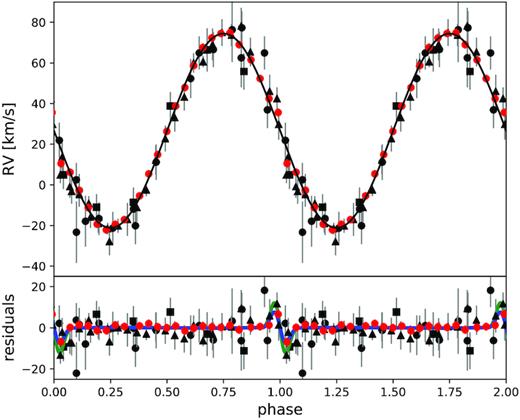
RV of J08205+0008 folded on the orbital period. The residuals are shown together with a prediction of the Rossiter–McLaughlin effect using the parameters derived in this paper in blue and a model with a higher rotational velocity assuming bound rotation in green. The RVs were determined from spectra obtained with XSHOOTER (red circles), UVES (black triangles), EFOSC2 (black circles), and SDSS (black rectangles). The EFOSC2 and SDSS RVs have been corrected by a systematic shift (see the text for details).
Except for the corrected system velocity, the revised orbital parameters of J08205+0008 are consistent with those determined by Geier et al. (2011c) (|$P=0.096\pm 0.001\, {\rm d}$|, K = 47.4 ± 1.9 km s−1), but much more precise.
3.7 Eclipse timing
Since the discovery that J08205+00008 is an eclipsing binary in 2009 November, we have monitored the system regularly using BUSCA mounted at the 2.2-m telescope in Calar Alto, Spain, ULTRACAM and the 1 m in Sutherland Observatory (SAAO), South Africa. Such studies have been performed for several post-common envelope systems with sdB or WD primaries and M dwarf companions (see Lohr et al. 2014, for a summary). In many of those systems period changes have been found.
Together with the discovery data observed with Merope at the Mercator telescope on La Palma (Geier et al. 2011c), it was possible to determine timings of the primary eclipse over more than 10 yr, as described in Sections 2.4 and 2.5. All measured mid-eclipse times can be found in Table G1.
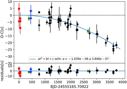
(O–C) diagram for J08205+0008 using eclipse times observed with Merope (red squares), BUSCA (blue diamonds), ULTRACAM (green triangles), and the SAAO-1-m/1.9-m telescope (black circles). The solid line represents a fit of a parabola to account for the period change of the orbital period. The derived quadratic term is given in the legend. The parameters of the fit are provided in the legend. In the lower panel, the residuals between the observations and the best fit are shown.
3.8 Light-curve modelling
With the new very high-quality ULTRACAM u′g′r′ light curves, we repeated the light-curve analysis of (Geier et al. 2011c) obtaining a solution with much smaller errors. For the modelling of the light curve we used lcurve, a code written to model detached and accreting binaries containing a WD (for details, see Copperwheat et al. 2010). It has been used to analyse several detached WD–M dwarf binaries (e.g. Parsons et al. 2010). Those systems show very similar light curves with very deep, narrow eclipses and a prominent reflection effect, if the primary is a hot WD. Therefore, lcurve is ideally suited for our purpose.
The code calculates monochromatic light curves by subdividing each star into small elements with a geometry fixed by its radius as measured along the line from the centre of one star towards the centre of the companion. The flux of the visible elements is always summed up to get the flux at a certain phase. A number of different effects that are observed in compact and normal stars are considered, for example, Roche distortions observed when a star is distorted from the tidal influence of a massive, close companion, as well as limb-darkening and gravitational darkening. Moreover, lensing and Doppler beaming, which are important for very compact objects with close companions, can be included. The Roemer delay, which is a light traveltime effect leading to a shift between primary and secondary eclipse times due to stars of different mass orbiting each other and changing their distance to us, and asynchronous orbits can be considered. The latter effects are not visible in our light curves and can hence be neglected in our case.
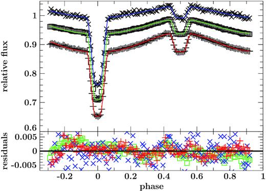
ULTRACAM u′g′r′ light curves of J08205+0008 together with the best fit of the most consistent solution. The light curves in the different filters have been shifted for better visualization. The lower panel shows the residuals. The deviation of the light curves from the best fit is probably due to the fact that the comparison stars cannot completely correct for atmospheric effects due to the different colour and the crude reflection effect model used in the analysis is insufficient to correctly describe the shape of the reflection effect.
As the light-curve model contains many parameters, not all of them independent, we fixed as many parameters as possible (see Table 2). The temperature of the sdB was fixed to the temperature determined from the spectroscopic fit. We used the values determined by the co-added XSHOOTER spectra, as they have higher S/N. The gravitational limb-darkening coefficients were fixed to the values expected for a radiative atmosphere for the primary (von Zeipel 1924) and a convective atmosphere for the secondary (Lucy 1967) using a blackbody approximation to calculate the resulting intensities. For the limb darkening of the primary we adopted a quadratic limb-darkening law using the tables by Claret & Bloemen (2011). As the tables include only surface gravities up to log g = 5 we used the values closest to the parameters derived by the spectroscopic analysis.
Parameters of the light-curve fit of the ULTRACAM u’g’r’ band light curves.
| Band | u’ | g’ | r’ |
|---|---|---|---|
| Fixed parameters | |||
| q | 0.147 | ||
| P | 0.09624073885 | ||
| Teff, sdB | 25800 | ||
| x1, 1 | 0.1305 | 0.1004 | 0.0788 |
| x1, 2 | 0.2608 | 0.2734 | 0.2281 |
| g1 | 0.25 | ||
| g2 | 0.08 | ||
| Fitted parameters | |||
| i | 85.3 ± 0.6 | 85.6 ± 0.2 | 85.4 ± 0.3 |
| r1/a | 0.2772 ± 0.0029 | 0.2734 ± 0.0010 | 0.2748 ± 0.0014 |
| r2/a | 0.1322 ± 0.0018 | 0.1297 ± 0.0006 | 0.1304 ± 0.0008 |
| Teff, comp | 3000 ± 500 | 2900 ± 500 | 3200 ± 560 |
| Absorb | 1.54 ± 0.08 | 1.58 ± 0.03 | 2.08 ± 0.05 |
| x2 | 0.70 | 0.78 | 0.84 |
| T0 (MJD) | 57832.0355 | 57832.0354 | 57832.0354 |
| slope | -0.000968 | -0.002377 | 0.00013417 |
| |$\frac{L_1}{L_1+L_2}$| | 0.992578 | 0.98735 | 0.97592 |
As it is a well-separated binary, the two stars are approximately spherical, which means the light curve is not sensitive to the mass ratio. Therefore, we computed solutions with different, fixed mass ratios. To localize the best set of parameters, we used a simplex algorithm (Press et al. 1992) varying the inclination, the radii, the temperature of the companion, the albedo of the companion (absorb), the limb darkening of the companion, and the time of the primary eclipse to derive additional mid-eclipse times. Moreover, we also allowed for corrections of a linear trend, which is often seen in the observations of hot stars, as the comparison stars are often redder and so the correction for the airmass is often insufficient. This is given by the parameter ‘slope’. The model of the best fit is shown in Fig. 8 together with the observations and the residuals.
To get an idea about the degeneracy of parameters used in the light-curve solutions, as well as an estimation of the errors of the parameters we performed Markov Chain Monte Carlo (MCMC) computations with emcee (Foreman-Mackey et al. 2013) using the best solution we obtained with the simplex algorithm as a starting value varying the radii, the inclination, the temperature of the companion as well as the albedo of the companion. As a prior we constrained the temperature of the cool side of the companion to 3000 ± 500 K. Due to the large luminosity difference between the stars the temperature of the companion is not significantly constrained by the light curve. The computations were done for all three light curves separately.
For the visualization, we used the python package corner (see Fig. 9 Foreman-Mackey 2016). The results of the MCMC computations of the light curves of all three filters agree within the error (see Table 2). A clear correlation between both radii and the inclination is visible as well as a weak correlation of the albedo of the companion (absorb) and the inclination. This results from the fact that the companion is only visible in the combined flux due to the reflection effect and the eclipses and the amplitude of the reflection effect depends on the inclination, the radii, the separation, the albedo, and the temperatures. Looking at the χ2 of the temperature of the companion we see that all temperatures give equally good solutions showing that the temperature can indeed not be derived from the light-curve fit. The albedo we derived has, moreover, a value > 1, which has been found in other HW Vir systems as well and is due to the simplistic modelling of the reflection effect. The reason for the different distribution in the inclination is not clear to us. However, it is not seen in the other bands. It might be related to the insufficient correction of atmospheric effects by the comparison stars.
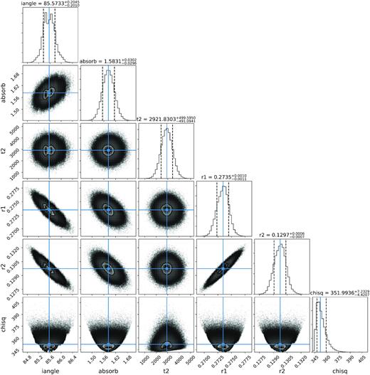
MCMC calculations showing the distributions of the parameter of the analysis of the ULTRACAM g’-band light curve.
3.9 Absolute parameters of J08205+00008
As explained before, we calculated solutions for different mass ratios (q = 0.11–0.20). We obtain equally good χ2 for all solutions, showing that the mass ratio cannot be constrained by the light-curve fit as expected. Hence, the mass ratio needs to be constrained differently. However, the separation, which can be calculated from the mass ratio, period, semi-amplitude of the RV curve and the inclination, is different for each mass ratio. The masses of both companions can then be calculated from the mass function. From the relative radii derived from the light-curve fit together with the separation, the absolute radii can be calculated. This results in different radii and masses for each mass ratio.
As stated before, the previous analysis of Geier et al. (2011c) resulted in two possible solutions: A post-RGB star with a mass of 0.25 |$\rm M_\odot$| and a core helium-burning star on the EHB with a mass of |$\rm 0.47\, M_\odot$|. From the analysis of the photometry together with the Gaia magnitudes (see Section 3.5), we get an additional good constraint on the radius of the sdB. Moreover, the surface gravity was derived from the fit to the spectrum. This can be compared to the mass and radius of the sdB (and a photometric log g: g = GM/R2) derived in the combined analysis of RV and light curves. This is shown in Fig. 10. We obtain a good agreement for of all three methods (spectroscopic, photometric, and parallax-based) for an sdB mass between 0.39 and 0.60 |$\rm M_\odot$|. This means that we can exclude the post-RGB solution. The position of J0820 in the Teff–log g diagram, which is shown in Fig. 2, gives us another constraint on the sdB mass. By comparing the atmospheric parameters of J08205+0008 to theoretical evolutionary tracks calculated by Han et al. (2002), it is evident that the position is not consistent with sdB masses larger than |$\sim 0.50\, \rm M_\odot$|, which we, therefore, assume as the maximum possible mass for the sdB.
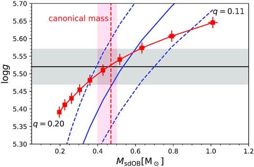
Mass of the sdB versus the photometric log g for J08205+0008 for different mass ratios from 0.11 to 0.20 in steps of 0.01 (red solid line). The parameters were derived by combining the results from the analysis of the light and RV curves. The grey area marks the spectroscopic log g that was derived from the spectroscopic analysis. The blue dashed lines indicate the log g derived by the radius from the SED fitting and the Gaia distance for different sdB masses. The red area marks the mass range for the sdB for which we get a consistent solution by combining all different methods. The red vertical line represents the solution for a canonical mass sdB.
Accordingly, we conclude that the solution that is most consistent with all different analysis methods is an sdB mass close to the canonical mass (|$0.39\!-\!0.50\, \rm M_\odot$|). For this solution, we have an excellent agreement of the parallax radius with the photometric radius only, if the parallax offset of −0.029 mas suggested by Lindegren et al. (2018) is used. Otherwise the parallax-based radius is too large. The companion has a mass of |$0.061\!-\!0.71\, \rm M_\odot$|, which is just below the limit for hydrogen-burning. Our final results can be found in Table 3. The mass of the companion is below the hydrogen-burning limit and the companion is hence most likely a massive BD.
Parameters of J08205+0008.
| Spectroscopic parameters | ||
|---|---|---|
| γ | (|${\rm km\, s^{-1}}$|) | 26.5 ± 0.4 |
| K1 | (|${\rm km\, s^{-1}}$|) | 47.8 ± 0.4 |
| f(M) | (M⊙) | 0.0011 ± 0.0001 |
| Teff, sdB | (K) | 25800 ± 290* |
| log g, sdB | 5.52 ± 0.04* | |
| log n(He) | −2.07 ± 0.04* | |
| vsin i | (|${\rm km\, s^{-1}}$|) | 65.9 ± 0.1† |
| a | (|$\rm R_\odot$|) | 0.71 ± 0.02 |
| M1 | (M⊙) | 0.39–0.50 |
| M2 | (M⊙) | 0.061–0.071 |
| Photometric parameters | ||
| T0 | (BJDTDB) | 2455165.709211(1) |
| P | (d) | 0.09624073885(5) |
| |$\dot{P}$| | dd−1 | −3.2(8) × 10−12 |
| i | (°) | 85.6 ± 0.3 |
| R1 | (R⊙) | 0.194 ± 0.008 |
| R2 | (R⊙) | 0.092 ± 0.005 |
| log g | 5.52 ± 0.03 | |
| SED fitting | ||
| ϖGaia | (mas) | 0.6899 ± 0.0632† |
| E(B − V) | (mag) | 0.040 ± 0.010† |
| θ | (10−12 rad) | 6.22 ± 0.15* |
| RGaia | (R⊙) | 0.200|$^{+0.021\ast }_{-0.018}$| |
| MGaia | (M⊙) | 0.48|$^{+0.12\ast }_{-0.09}$| |
| log (LGaia/L⊙) | 16|$^{+3.6\ast }_{-2.8}$| | |
We also investigated the mass and radius of the companion and compared it to theoretical calculations by Baraffe et al. (2003) and Chabrier & Baraffe (1997) as shown in Fig. 11. It is usually assumed that the progenitor of the sdB was a star with about |$1\!-\!2\, \rm M_\odot$| (Heber 2009, 2016). Therefore, we expect that the system is already quite old (5–10 Gyr). For the solutions in our allowed mass range the measured radius of the companion is about 20 per cent larger than expected from theoretical calculations. Such an effect, called inflation, has been observed in different binaries and also planetary systems with very close Jupiter-like planets. A detailed discussion will be given later. This effect has already been observed in other hot subdwarf close binary systems (e.g. Schaffenroth et al. 2015).
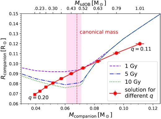
Comparison of theoretical mass–radius relations of low-mass stars (Baraffe et al. 2003; Chabrier & Baraffe 1997) to results from the light-curve analysis of J08205+0008. We used tracks for different ages of 1 Gyr (dashed), 5 Gyr (dotted–dashed), and 10 Gyr (dotted). Each red square together with the errors represents a solution from the light-curve analysis for a different mass ratio (q = 0.11–0.20 in steps of 0.01). The red vertical line represents the solution for a canonical mass sdB. The red area marks the mass range of the companion corresponding to the mass range we derived for the sdB.
However, if the system would still be quite young with an age of about 1 Gyr, the companion would not be inflated. We performed a kinematic analysis to determine the Galactic population of J08205+0008. As seen in Fig. 12, the sdB binary belongs to the thin disc where star formation is still ongoing and could therefore indeed be as young as 1 Gyr, if the progenitor was a |$2\, \rm M_\odot$| star. About half of the sdO/Bs at larger distances from the Galactic plane (0.5 kpc) are found in the thin disc (Martin et al. 2017). However, it is unclear whether a BD companion can eject the evelope from such a massive 2 |$\rm M_{\odot }$| star. Hydrodynamical simulations performed by Kramer et al. (2020) indicate that a BD companion of |$\sim\! 0.05\!-\!0.08\, \rm M_\odot$| might just be able to eject the CE of a lower mass (|$1\, \rm M_\odot$|) red giant.
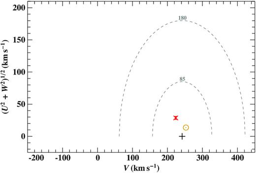
Toomre diagram of J08205+0008: the quantity V is the velocity in direction of Galactic rotation, U towards the Galactic centre, and W perpendicular to the Galactic plane. The two dashed ellipses mark boundaries for the thin (85 km s−1) and thick disc (180 km s−1) following Fuhrmann (2004). The red cross marks J08205+0008, the yellow circled dot the Sun, and the black plus the local standard of rest. The location of J08205+0008 in this diagram clearly hints at a thin disc membership.
4 DISCUSSION
4.1 Tidal synchronization of sdB+dM binaries
In close binaries, the rotation of the components is often assumed to be synchronized to their orbital motion. In this case, the projected rotational velocity can be used to put tighter constraints on the companion mass. Geier et al. (2010) found that assuming tidal synchronization of the subdwarf primaries in sdB binaries with orbital periods of less than |$\simeq 1.2\, {\rm d}$| leads to consistent results in most cases. In particular, all the HW Vir type systems analysed in the Geier et al. (2010) study turned out to be synchronized.
Due to the short period of this binary, the sdB should spin with |$v_{\rm syncro}\simeq 102\, {\rm km\, s^{-1}}$| similar to the other known systems (see Geier et al. 2010, and references therein).
Other observational results in recent years also indicate that tidal synchronization of the sdB primary in close sdB+dM binaries is not always established in contrast to the assumption made by Geier et al. (2010). New theoretical models for tidal synchronization (Preece, Tout & Jeffery 2018, 2019) even predict that none of the hot subdwarfs in close binaries should rotate synchronously with the orbital period.
From the observational point of view, the situation appears to be rather complicated. Geier et al. (2010) found the projected rotational velocities of the two short-period (|$P=0.1\!-\!0.12\, {\rm d}$|) HW Vir systems HS 0705+6700 and the prototype HW Vir to be consistent with synchronization. Charpinet et al. (2008) used the splitting of the pulsation modes to derive the rotation period of the pulsating sdB in the HW Vir-type binary PG 1336−018 and found it to be consistent with synchronized rotation. This was later confirmed by the measurement of the rotational broadening (Geier et al. 2010).
However, the other two sdBs with BD companions J162256+473051 and V2008−1753 (Schaffenroth et al. 2014a, 2015) have even shorter periods of only 0.07 d and both show subsynchronous rotation with 0.6 and 0.75 of the orbital period, respectively, just like J0820+0008. AA Dor on the other hand, which has a companion very close to the hydrogen-burning limit and a longer period of 0.25 d, seems to be synchronized (Vučković et al. 2016, and references therein), but it has already evolved beyond the EHB and is therefore older and has had more time to synchronize.
Pablo, Kawaler & Green (2011) and Pablo et al. (2012) studied three pulsating sdBs in reflection effect sdB+dM binaries with longer periods and again used the splitting of the pulsation modes to derive their rotation periods (|$P\simeq 0.39\!-\!0.44\, {\rm d}$|). All three sdBs rotate much slower than synchronized. But also in this period range the situation is not clear, since a full asteroseismic analysis of the sdB+dM binary Feige 48 (|$P\simeq 0.38\, {\rm d}$|) is consistent with synchronized rotation.
Since synchronization time-scales of any kind (Geier et al. 2010) scale dominantely with the orbital period of the close binary, these results seem puzzling. Especially since the other relevant parameters such as mass and structure of the primary or companion mass are all very similar in sdB+dM binaries. They all consist of core-helium-burning stars with masses of |$\sim 0.5\, \mathrm{ M}_{\odot }$| and low-mass companions with masses of |$\sim 0.1\, \mathrm{ M}_{\odot }$|. And yet five of the analysed systems appear to be synchronized, while six rotate slower than synchronized without any significant dependence on companion mass or orbital period. This fraction, which is of course biased by complicated selection effects, might be an observational indication that the synchronization time-scales of such binaries are of the same order as the evolutionary time-scales.
It has to be pointed out that although evolutionary tracks of EHB stars exist, the accuracy of the derived observational parameters (usually Teff and log g) is not high enough to determine their evolutionary age on the EHB by comparison with those tracks as accurate as it can be done for other types of stars (see Fig. 2). As shown in Fig. 2, the position of the EHB is also dependent on the core and envelope mass and so it is not possible to find a unique track to a certain position in the Teff–log g diagram and in most sdB systems the mass of the sdB is not constrained accurately enough.
Lisker et al. (2005) showed that sdB stars move at linear speed over the EHB and so the distance from the zero-age EHB (ZAEHB) represents how much time the star already spent on the EHB. If we look at the position of the non-synchronized against the position of the synchronized systems in the Teff–log g diagram (Fig. 13), it is obvious that all the systems, which are known to be synchronized, appear to be older. There also seems to be a trend that systems with a higher ratio of rotational to orbital velocity are further away from the ZAEHB. This means that the fraction of rotational to orbital period might even allow an age estimate of the sdB.
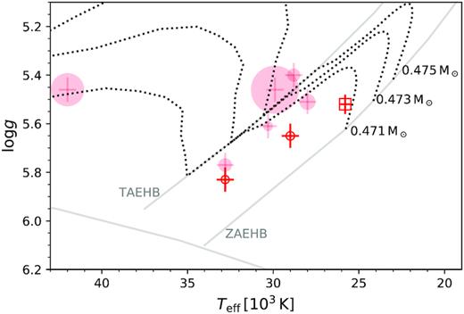
Teff–log (g) diagram for the sdB+dM systems with known rotational periods mentioned in Section 4.1. The filled symbols represent synchronized systems, the open symbols, systems which are known to be non-synchronized. The square marks the position of J08205+0008. The sizes of the symbols scale with the orbital period, with longer periods having larger symbols. Plotted error bars are the estimated parameter variations due to the reflection effect, as found, for example, in Schaffenroth et al. (2013). The ZAEHB and TAEHB for a canonical mass sdB as well as evolutionary tracks for a canonical mass sdB with different envelope masses from Dorman et al. (1993) are also shown.
The fact that the only post-EHB HW Vir system with a candidate substellar companion in our small sample (AA Dor) appears to be synchronized, while all the other HW Vir stars with very low-mass companions and shorter periods are not, fits quite well in this scenario. This could be a hint to the fact that for sdB+dM systems the synchronization time-scales are comparable to or even smaller than the lifetime on the EHB. Hot subdwarfs spend |$\sim 100\, {\rm Myr}$| on the EHB before they evolve to the post-EHB stage lasting |$\sim 10\, {\rm Myr}$|. So we would expect typical synchronization time-scales to be of the order of a few tens of millions of years, as we see both synchronized and unsynchronized systems.
4.2 A new explanation for the period decrease
There are different mechanisms of angular momentum loss in close binaries leading to a period decrease: gravitational waves, mass transfer (which can be excluded in a detached binary), or magnetic braking (see Qian et al. 2008). Here, we propose that tidal synchronization can also be an additional mechanism to decrease the orbital period of a binary.
From the rotational broadening of the stellar lines (see Section 4.1), we derived the rotational velocity of the subdwarf to be about half of what would be expected from the sdB being synchronized to the orbital period of the system. This means that the sdB is currently spun up by tidal forces until synchronization is reached causing an increase in the rotational velocity. As the mass of the companion is much smaller than the mass of the sdB, we assume synchronization for the companion.
From this equation, we can clearly see that rotational velocity change depends on the masses of both stars, the radius of the primary, the orbital velocity change, and the current orbital velocity. An increasing rotational velocity causes an increasing orbital velocity and hence a period decrease.
4.3 Synchronization time-scale
This means that this effect could significantly add to the observed period decrease. The fact that the synchronized systems appear to be older than the non-synchronized ones confirms that the synchronization time-scale is of the expected order of magnitude and it is possible that we might indeed measure the synchronization time-scale.
As mentioned before, Preece et al. (2018) predict that the synchronization time-scales are much longer than the lifetime on the EHB and that none of the HW Vir systems should be synchronized. Preece et al. (2019) investigated also the special case of NY Vir, which was determined to be synchronized from spectroscopy and asteroseismolgy, and came to the conclusion that they cannot explain, why it is synchronized. They proposed that maybe the outer layers of the sdB were synchronized during the common envelope phase. However, observations show that synchronized sdB+dM systems are not rare, but that synchronization occurs most likely during the phase of helium-burning, which shows that synchronization theory is not yet able to predict accurate synchronization time-scales.
4.4 Orbital period variations in HW Vir systems
As mentioned before, there are several mechanisms that can explain period changes in HW Vir systems. The period change due to gravitational waves is usually very small in HW Vir systems and would only be observable after observations for many decades (e.g. Kilkenny 2014). Using the equation given in Kupfer et al. (2020) with the system parameters derived in this paper, we predict an orbital period decay due to gravitational waves of |$\dot{P}=\rm- 4.5e{-}14\, \rm ss^{-1}$|. The observed change in orbital period is hence about 100 times higher than expected by an orbital decay due to gravitational waves.
HW Vir and NY Vir have also been observed to show a period decrease of the same order of magnitude (Qian et al. 2008; Kilkenny 2014) but have been found to rotate (nearly) synchronously. Both also show additionally to the period decrease a long-period sinusoidal signal (Lee et al. 2009, 2014). These additional variations in the O–C diagram have been interpreted as caused by circumbinary planets in both cases, however the solutions were not confirmed with observations of longer baselines. Observations of more than one orbital period of the planet would be necessary to confirm it. The period decrease was explained to be caused by angular momentum loss due to magnetic stellar wind braking.
Following the approach of Qian et al. (2007), we calculated the relation between the mass-loss rate and the Alfvén radius that would be required to account for the period decrease in J08205+0008 due to magnetic braking. This is shown in Fig. 14. Using the tidally enhanced mass-loss rate of Tout & Eggleton (1988) we derive that an Alfvén radius of |$75\, \rm R_\odot$| would be required to cause the period decrease we measure, much larger than the Alfvén radius of the Sun. This shows that, as expected, the effect of magnetic braking in a late M dwarf or massive BD is very small at best and cannot explain the period decrease we derive.
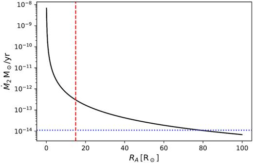
Correlation between the Alfvén radius and the mass-loss rate for the companion of J08205+0008. The red dashed line marks the Alfvén radius for the Sun, the blue dotted line indicates the tidally enhanced mass-loss rate determined using the parameters of the sdB using the formula of Tout & Eggleton (1988).
Bours et al. (2016) made a study of close WD binaries and observed that the amplitude of eclipse arrival time variations in K dwarf and early M dwarf companions is much larger than in late M dwarf, BD or WD companions, which do not show significant orbital period variations. They concluded that these findings are in agreement with the so-called Applegate mechanism, which proposes that variability in the binary orbits can be driven by magnetic cycles in the secondary stars. In all published HW Vir systems with a longer observational baseline of several years quite large period variations on the order of minutes have been detected (see Zorotovic & Schreiber 2013; Pulley et al. 2018, for an overview), with the exception of AA Dor (Kilkenny 2014), which still shows no sign of period variations after a baseline of about 40 yr. Also the orbital period decrease in J08205+0008 is on the order of seconds and has only been found after 10 yr of observation and no additional sinusoidal signals have been found as seen in many of the other systems. This confirms that the findings of Bours et al. (2016) apply to close hot subdwarf binaries with cool companions. The fact that the synchronized HW Vir system AA Dor does not show any period variations also confirms our theory that the period variations in HW Vir systems with companions close to the hydrogen-burning limit might be caused by tidal synchronization. In higher mass M dwarf companions, the larger period variations are likely caused by the Applegate mechanism and the period decrease can be caused dominantly by magnetic braking and additionally tidal synchronization.
It seems that orbital period changes in HW Vir systems are still poorly understood and have also not been studied observationally to the full extent. More observations over long time spans of synchronized and non-synchronized short-period sdB binaries with companions of different masses will be necessary to understand synchronization and orbital period changes of hot subdwarf binaries. Most likely it cannot be explained with just one effect and is likely an interplay of different effects.
4.5 Inflation of brown dwarfs and low-mass M dwarfs in eclipsing WD or sdB binaries
Close BD companions that eclipse main-sequence stars are rare, with only 23 known to date (Carmichael et al. 2020). Consequently, BD companions to the evolved form of these systems are much rarer with only three (including J08205+0008) known to eclipse hot subdwarfs, and three known to eclipse WDs. These evolved systems are old (> 1 Gyr), and the BDs are massive, and hence not expected to be inflated (Thorngren & Fortney 2018).
Surprisingly, of the three hot subdwarfs with BD companions, J08205+0008 is the one that receives the least irradiation – almost half that received by V2008−1753 and SDSSJ162256.66+473051.1, both of which have hotter primaries (32000 K, 29000 K) and shorter periods (∼1.6 h) than J08205+0008. This suggests that more irradiation, and more irradiation at shorter wavelengths does not equate to a higher level of inflation of a BD. Indeed this finding is consistent with that for BDs irradiated by WDs, where the most irradiated object with a measured radius is SDSS J1205-0242B, in a 71.2 min orbit around a 23681 K WD and yet the BD is not inflated (Parsons et al. 2017). The BD in this system only receives a hundredth of the irradiation that J08205+0008 does. However, WD1032+011, an old WD (Teff ∼ 10 000 K) with a high-mass BD companion (0.0665 M⊙) does appear to be inflated (Casewell et al. 2020). As can be seen from Fig. 15, the majority of the low-mass BDs (M < 35 MJup) are inflated, irrelevant of how much irradiation they receive. For the few old (5–10 Gyr), higher mass inflated BDs, the mechanism leading to the observed inflation is not yet understood.
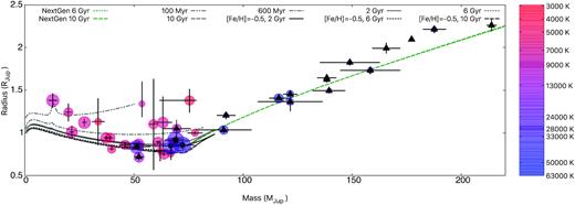
All known eclipsing binary WDs with detached BD (triangles: Parsons et al. 2017; Littlefair et al. 2014) and late M dwarf companions (triangles) from Parsons et al. (2018), hot subdwarfs with eclipsing BD companions (circles: Schaffenroth et al. 2014b, 2015), and all known eclipsing BD companions to main-sequence stars (+: Carmichael et al. 2020). J08205+0008 is plotted as the filled square. The colour is proportional to the effective temperature of the primary in each system and the coloured circle size is proportional to the amount of total incident radiation the secondary receives. Also shown are the Sonora Bobcat BD evolutionary models3 of Marley et al. (in preparation) for solar and subsolar metallicity and the NextGen models (Baraffe et al. 1997).
4.6 Previous and future evolution of the system
As stated before, stars with a cool, low-mass companion sitting on the EHB are thought to have formed by a common-envelope phase from a progenitor of up to two solar mass on the RGB. Due to the large mass ratio only unstable mass transfer is possible. If the mass transfer happened at the tip of the RGB, a core-helium-burning object with about |$0.5\, \rm M_\odot$| will be formed. If the mass transfer happened earlier then the core of the progenitor has not enough mass to start He-core-burning and the pre-He WD will move to the WD cooling track crossing the EHB. Our analysis of J08205+0008 showed that a low-mass solution (|$0.25\, \mathrm{ M}_\odot$|, as discussed previously) can be excluded and that the primary star is indeed currently a core He-burning object.
Systems with a mass ratio q = M2/M1 < 2/3, with M1 being the mass of the accretor, are assumed to be able to undergo stable mass transfer. Our system has a mass ratio of 0.147 ≪ 2/3. The subdwarf will already have evolved to a WD and a cataclysmic variable will be formed. It is expected that the period of an accreting binary with a hydrogen-rich donor star will decrease until a minimum period of ≃70 min is reached at a companion mass around |$0.06\, \mathrm{ M}_\odot$| and the period will increase again afterwards (Nelson et al. 2018). Such systems are called period bouncers. Our system comes into contact already close to the minimum period and should hence increase the period when the mass transfer starts.
The future of the system depends completely on the period evolution. A longer baseline of observations of this system is necessary to confirm that the period decrease is indeed stable and caused by the tidal synchronization.
5 CONCLUSION AND SUMMARY
The analysis of J08205+0008 with higher quality data from ESO-VLT/XSHOOTER, ESO-VLT/UVES, and ESO-NTT/ULTRACAM allowed us to constrain the masses of the sdB and the companion much better by combining the analysis of the RV and the light curves. We determine an sdB mass of |$0.39\!-\!0.50\, \rm M_\odot$| consistent with the canonical mass and a companion mass of |$0.061-0.071\, \rm M_\odot$| close to the hydrogen-burning limit. Therefore, we confirm that the companion is likely be a massive BD.
The atmospheric parameters and abundances show that J08205+0008 is a typical sdB and comparison with stellar evolution tracks suggest that the mass has to be less than |$0.50\, \mathrm{ M}_\odot$| consistent with our solution and also the mass derived by a spectrophotometric method using Gaia parallaxes and the SED derived in the secondary eclipse, where the companion is not visible.
If the sdB evolved from a |$1\, \rm M_\odot$| star, the age of the system is expected to be around 10 Gyr. In this case, the radius of the BD companion is about 20 per cent inflated compared to theoretical calculations. Such an inflation is observed in several sdB/WD+dM/BD systems but not understood yet. However, the inflation seems not to be caused by the strong irradiation. The sdB binary belongs to the thin disc, as do about half of the sdB at this distance from the Galactic plane. This means that they also could be young, if they have evolved from a more massive progenitor. Then, we get a consistent solution without requiring inflation of the companion. However, a BD companion might not be able to remove the envelope of a more massive progenitor.
We detected a significant period decrease in J0820+0008. This can be explained by the spin-up of the sdB due to tidal sychronization. We calculated the synchronization time-scale to 4 Myr well within the lifetime on the EHB. The investigation of the parameters of all known Vir systems with rotational periods (see Section 4.1) shows that the synchronized systems tend to be older, showing that the synchronization time-scale seems to be comparable but smaller than the lifetime on the EHB in contrast to current synchronization theories.
By investigating the known orbital period variations in HW Vir systems, we can confirm the findings by Bours et al. (2016) that period variations in systems with higher mass M dwarf companions seem to be larger. Hence, we conclude that the large period variations in those systems are likely caused by the Applegate mechanism and the observed period decreases dominantly by magnetic braking. In lower mass companions close to the hydrogen-burning limit, on the other hand, tidal synchronization spinning up the sdB could be responsible for the period decrease, allowing us to derive a synchronization time-scale.
The results of our analysis are limited by the precision of the available trigonometric parallax. As the Gaia mission proceeds, the precision and accuracy of the trigonometric parallax will improve, which will narrow down the uncertainties of the stellar parameters. A very important goal is to detect spectral signatures from the companion and to measure the RV curve of the companion. We failed to do so, because the infrared spectra at hand are of insufficient quality. The future IR instrumentation on larger telescopes, such as the ESO-ELT, will be needed. A high precision measurement of the RV curves of both components will then allow us to derive an additional constraint on mass and radius from the difference of the stars’ gravitational redshifts (Vos et al. 2013). Such measurements will give an independent determination of the nature of the companion and will help to test evolutionary models for low mass star near the hydrogen-burning limit via the mass–radius relation.
The combination of many different methods allowed us to constrain the masses of both components much better without having to assume a canonical mass for the sdB. This is only the fourth HW Vir system for which this is possible.
ACKNOWLEDGEMENTS
DS is supported by the Deutsche Forschungsgemeinschaft (DFG) under grant HE 1356/70-1 and IR190/1-1. VS is supported by the Deutsche Forschungsgemeinschaft, DFG through grant GE 2506/9-1. SLC is supported by an STFC (Science and Technology Facilities Council) Ernest Rutherford Fellowship ST/R003726/1. DK thanks the SAAO for generous allocations of telescope time and the National Research Foundation of South Africa and the University of the Western Cape for financial support. VSD, SPL, and ULTRACAM are supported by the STFC. We thank J. E. Davis for the development of the slxfig module, which has been used to prepare figures in this work. matplotlib (Hunter 2007) and numpy (van der Walt, Colbert & Varoquaux 2011) were used in order to prepare figures in this work. This work has made use of data from the European Space Agency (ESA) mission Gaia (https://www.cosmos.esa.int/gaia), processed by the Gaia Data Processing and Analysis Consortium (DPAC, https://www.cosmos.esa.int/web/gaia/dpac/consortium). Funding for the DPAC has been provided by national institutions, in particular the institutions participating in the Gaia Multilateral Agreement. Based on observations at the Cerro Paranal Observatory of the European Southern Observatory (ESO) in Chile under the program IDs 087.D-0185(A), and 098.C-0754(A). Based on observations at the La Silla Observatory of the ESO in Chile under the program IDs 082.D-0649(A), 084.D-0348(A), and 098.D-679. This paper uses observations made at the South African Astronomical Observatory. We made extensive use of NASAs Astrophysics Data System Abstract Service (ADS) and the SIMBAD and VizieR database, operated at CDS, Strasbourg, France.
DATA AVAILABILITY STATEMENT
Most data are incorporated into the article and its appendix. All other data (light curves and spectra) are available on request.
Footnotes
Fitzpatrick et al. (2019) use E(44 − 55), the monochromatic equivalent of the usual E(B − V) in the Johnson system, using the wavelengths λ = 4400 and 5000 Å, respectively. In fact, E(44 − 55) is identical to E(B − V) for high effective temperatures as determined for J08205+0008.
REFERENCES
APPENDIX A: TELLURIC CORRECTION
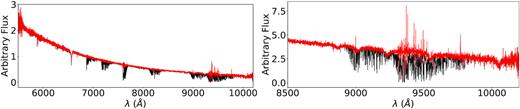
Left-hand panel: quality of telluric absorption correction for a full example spectrum of J08205+0008 taken with the VIS arm of the XSHOOTER spectrograph. The telluric absorption corrected spectrum (red) is shown in comparison with the original spectrum (black). Note that fluxes were scaled for illustrative purposes. Right-hand panel: same as left-hand panel, but for the spectral range of the hydrogen Paschen series.
APPENDIX B: ATMOSPHERIC MODEL PARAMETERS
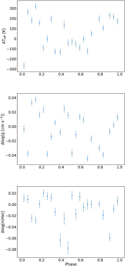
Change of the atmospheric parameters determined from the single XSHOOTER spectra plotted against the orbital phase. While the differences plotted on the y axes result from the subtraction of the best-fitting parameters derived from the co-added XSHOOTER spectrum from the determined parameters for the single spectra, the orbital phase was calculated based on the photometric solutions of T0 and P (see Table 3 for details). Due to the relatively weak reflection effect of less than 5 per cent, the variations measured for effective temperature (upper panel), surface gravity (middle panel), and helium abundance (lower panel) are of the order of the total uncertainties listed in Table 3 and therefore are not significant.
Model atoms for NLTE calculations used for the hybrid LTE/NLTE approach.
| Ion | Model atom |
|---|---|
| |$\mathrm{H\,{\small I}}$| | Przybilla & Butler (2004) |
| |$\mathrm{He\,{\small I}}$| | Przybilla (2005) |
| |$\mathrm{C\,{\small II}}$| | Nieva & Przybilla (2006), Nieva & Przybilla (2008) |
| |$\mathrm{N\,{\small II}}$| | Przybilla & Butler (2001)† |
| |$\mathrm{O\,{\small I/II}}$| | Przybilla et al. (2000), Becker & Butler (1988)† |
| |$\mathrm{Ne\,{\small I/II}}$| | Morel & Butler (2008)† |
| |$\mathrm{Mg\,{\small II}}$| | Przybilla et al. (2001) |
| |$\mathrm{Al\,{\small III}}$| | Przybilla (in prep.) |
| |$\mathrm{Si\,{\small II/III/IV}}$| | Przybilla & Butler (in prep.) |
| |$\mathrm{S\,{\small II/III}}$| | Vrancken, Butler & Becker (1996)† |
| |$\mathrm{Ar\,{\small II}}$| | Butler (in prep.) |
| |$\mathrm{Fe\,{\small II/III}}$| | Becker (1998), Morel et al. (2006)† |
Note:†Updated and corrected as described by Nieva & Przybilla (2012).
Hybrid LTE/NLTE model grid used for the quantitative spectral analysis of J08205+0008.
| Parameter | Grid size | Step size |
|---|---|---|
| Teff | 25 000 to 30 000 K | 1000 K |
| log (g) | 5.2 to 5.8 | 0.2 |
| log n(He) | −2.2 to −1.6 | 0.2 |
| log n(C) | −4.6 to −4.0 | 0.2 |
| log n(N) | −4.2 to −3.6 | 0.2 |
| log n(O) | −4.4 to −3.8 | 0.2 |
| log n(Ne) | −7.0 to −6.0 | 0.2 |
| log n(Mg) | −5.4 to −4.4 | 0.2 |
| log n(Al) | −7.0 to −6.0 | 0.2 |
| log n(Si) | −5.4 to −5.0 | 0.2 |
| log n(S) | −6.0 to −5.2 | 0.2 |
| log n(Ar) | −5.8 to −5.4 | 0.2 |
| log n(Fe) | −4.8 to −4.2 | 0.2 |
APPENDIX C: LINE FITS
APPENDIX D: LIST OF METAL LINES
List of selected metal lines in the co-added XSHOOTER and UVES spectra of J08205+0008.
| El. + ion. stage | λ (Å) | El. + ion. stage | λ (Å) | El. + ion. stage | λ (Å) | El. + ion. stage | λ (Å) |
|---|---|---|---|---|---|---|---|
| |$\mathrm{C\,{\small II}}$| | 3918.97 | |$\mathrm{N\,{\small II}}$| | 5686.21 | |$\mathrm{Al\,{\small III}}$| | 4512.565 | |$\mathrm{Fe\,{\small III}}$| | 3600.943 |
| |$\mathrm{C\,{\small II}}$| | 3920.68 | |$\mathrm{N\,{\small II}}$| | 5710.77 | |$\mathrm{Al\,{\small III}}$| | 5696.604 | |$\mathrm{Fe\,{\small III}}$| | 3603.890 |
| |$\mathrm{C\,{\small II}}$| | 4267.00 | |$\mathrm{N\,{\small II}}$| | 5927.81 | |$\mathrm{Al\,{\small III}}$| | 5722.730 | |$\mathrm{Fe\,{\small III}}$| | 3611.736 |
| |$\mathrm{C\,{\small II}}$| | 4267.26 | |$\mathrm{N\,{\small II}}$| | 5931.78 | |$\mathrm{Si\,{\small II}}$| | 3856.018 | |$\mathrm{Fe\,{\small III}}$| | 3999.325 |
| |$\mathrm{C\,{\small II}}$| | 5132.95 | |$\mathrm{N\,{\small II}}$| | 5940.24 | |$\mathrm{Si\,{\small II}}$| | 3862.595 | |$\mathrm{Fe\,{\small III}}$| | 4000.518 |
| |$\mathrm{C\,{\small II}}$| | 5133.28 | |$\mathrm{N\,{\small II}}$| | 5941.65 | |$\mathrm{Si\,{\small II}}$| | 4128.067 | |$\mathrm{Fe\,{\small III}}$| | 4005.573 |
| |$\mathrm{C\,{\small II}}$| | 5145.16 | |$\mathrm{N\,{\small II}}$| | 5952.39 | |$\mathrm{Si\,{\small II}}$| | 4130.893 | |$\mathrm{Fe\,{\small III}}$| | 4137.130 |
| |$\mathrm{C\,{\small II}}$| | 6151.265 | |$\mathrm{N\,{\small II}}$| | 5954.28 | |$\mathrm{Si\,{\small II}}$| | 6347.103 | |$\mathrm{Fe\,{\small III}}$| | 4139.350 |
| |$\mathrm{C\,{\small II}}$| | 6151.534 | |$\mathrm{N\,{\small II}}$| | 6150.75 | |$\mathrm{Si\,{\small II}}$| | 6371.359 | |$\mathrm{Fe\,{\small III}}$| | 4140.482 |
| |$\mathrm{C\,{\small II}}$| | 6461.95 | |$\mathrm{N\,{\small II}}$| | 6482.05 | |$\mathrm{Si\,{\small III}}$| | 3590.465 | |$\mathrm{Fe\,{\small III}}$| | 4164.916 |
| |$\mathrm{C\,{\small II}}$| | 6578.05 | |$\mathrm{N\,{\small II}}$| | 6610.56 | |$\mathrm{Si\,{\small III}}$| | 3806.526 | |$\mathrm{Fe\,{\small III}}$| | 4194.051 |
| |$\mathrm{C\,{\small II}}$| | 6582.88 | |$\mathrm{O\,{\small I}}$| | 7771.94 | |$\mathrm{Si\,{\small III}}$| | 3806.7 | |$\mathrm{Fe\,{\small III}}$| | 4210.674 |
| |$\mathrm{C\,{\small II}}$| | 6779.94 | |$\mathrm{O\,{\small I}}$| | 7774.17 | |$\mathrm{Si\,{\small III}}$| | 3806.779 | |$\mathrm{Fe\,{\small III}}$| | 4222.271 |
| |$\mathrm{C\,{\small II}}$| | 6780.59 | |$\mathrm{O\,{\small I}}$| | 7775.39 | |$\mathrm{Si\,{\small III}}$| | 3924.468 | |$\mathrm{Fe\,{\small III}}$| | 4248.773 |
| |$\mathrm{C\,{\small II}}$| | 6783.91 | |$\mathrm{O\,{\small I}}$| | 8446.25 | |$\mathrm{Si\,{\small III}}$| | 4552.622 | |$\mathrm{Fe\,{\small III}}$| | 4261.391 |
| |$\mathrm{C\,{\small II}}$| | 6791.47 | |$\mathrm{O\,{\small I}}$| | 8446.36 | |$\mathrm{Si\,{\small III}}$| | 4567.84 | |$\mathrm{Fe\,{\small III}}$| | 4273.372 |
| |$\mathrm{C\,{\small II}}$| | 6800.69 | |$\mathrm{O\,{\small I}}$| | 8446.76 | |$\mathrm{Si\,{\small III}}$| | 4574.757 | |$\mathrm{Fe\,{\small III}}$| | 4273.409 |
| |$\mathrm{C\,{\small II}}$| | 7231.33 | |$\mathrm{O\,{\small II}}$| | 3390.21 | |$\mathrm{Si\,{\small III}}$| | 4716.654 | |$\mathrm{Fe\,{\small III}}$| | 4286.091 |
| |$\mathrm{C\,{\small II}}$| | 7236.42 | |$\mathrm{O\,{\small II}}$| | 3712.74 | |$\mathrm{Si\,{\small III}}$| | 4813.333 | |$\mathrm{Fe\,{\small III}}$| | 4286.128 |
| |$\mathrm{C\,{\small II}}$| | 7237.17 | |$\mathrm{O\,{\small II}}$| | 3727.32 | |$\mathrm{Si\,{\small III}}$| | 4819.631 | |$\mathrm{Fe\,{\small III}}$| | 4286.164 |
| |$\mathrm{N\,{\small II}}$| | 3328.72 | |$\mathrm{O\,{\small II}}$| | 3911.96 | |$\mathrm{Si\,{\small III}}$| | 4819.712 | |$\mathrm{Fe\,{\small III}}$| | 4296.814 |
| |$\mathrm{N\,{\small II}}$| | 3329.70 | |$\mathrm{O\,{\small II}}$| | 3912.12 | |$\mathrm{Si\,{\small III}}$| | 4819.814 | |$\mathrm{Fe\,{\small III}}$| | 4296.851 |
| |$\mathrm{N\,{\small II}}$| | 3330.32 | |$\mathrm{O\,{\small II}}$| | 4069.62 | |$\mathrm{Si\,{\small III}}$| | 4828.95 | |$\mathrm{Fe\,{\small III}}$| | 4304.748 |
| |$\mathrm{N\,{\small II}}$| | 3331.31 | |$\mathrm{O\,{\small II}}$| | 4069.88 | |$\mathrm{Si\,{\small III}}$| | 4829.03 | |$\mathrm{Fe\,{\small III}}$| | 4304.767 |
| |$\mathrm{N\,{\small II}}$| | 3437.14 | |$\mathrm{O\,{\small II}}$| | 4072.16 | |$\mathrm{Si\,{\small III}}$| | 4829.111 | |$\mathrm{Fe\,{\small III}}$| | 4310.355 |
| |$\mathrm{N\,{\small II}}$| | 3995.00 | |$\mathrm{O\,{\small II}}$| | 4075.86 | |$\mathrm{Si\,{\small III}}$| | 4829.214 | |$\mathrm{Fe\,{\small III}}$| | 4419.596 |
| |$\mathrm{N\,{\small II}}$| | 4035.08 | |$\mathrm{O\,{\small II}}$| | 4132.80 | |$\mathrm{Si\,{\small III}}$| | 5696.49 | |$\mathrm{Fe\,{\small III}}$| | 4649.271 |
| |$\mathrm{N\,{\small II}}$| | 4041.31 | |$\mathrm{O\,{\small II}}$| | 4185.44 | |$\mathrm{Si\,{\small III}}$| | 5739.73 | |$\mathrm{Fe\,{\small III}}$| | 5063.421 |
| |$\mathrm{N\,{\small II}}$| | 4043.53 | |$\mathrm{O\,{\small II}}$| | 4189.58 | |$\mathrm{S\,{\small II}}$| | 3613.03 | |$\mathrm{Fe\,{\small III}}$| | 5073.903 |
| |$\mathrm{N\,{\small II}}$| | 4176.16 | |$\mathrm{O\,{\small II}}$| | 4189.79 | |$\mathrm{S\,{\small II}}$| | 5201.027 | |$\mathrm{Fe\,{\small III}}$| | 5086.701 |
| |$\mathrm{N\,{\small II}}$| | 4199.98 | |$\mathrm{O\,{\small II}}$| | 4366.89 | |$\mathrm{S\,{\small II}}$| | 5201.379 | |$\mathrm{Fe\,{\small III}}$| | 5194.160 |
| |$\mathrm{N\,{\small II}}$| | 4227.74 | |$\mathrm{O\,{\small II}}$| | 4395.93 | |$\mathrm{S\,{\small II}}$| | 5212.267 | |$\mathrm{Fe\,{\small III}}$| | 5272.369 |
| |$\mathrm{N\,{\small II}}$| | 4237.05 | |$\mathrm{O\,{\small II}}$| | 4414.46 | |$\mathrm{S\,{\small II}}$| | 5212.62 | |$\mathrm{Fe\,{\small III}}$| | 5272.900 |
| |$\mathrm{N\,{\small II}}$| | 4241.76 | |$\mathrm{O\,{\small II}}$| | 4414.90 | |$\mathrm{S\,{\small II}}$| | 5345.712 | |$\mathrm{Fe\,{\small III}}$| | 5272.975 |
| |$\mathrm{N\,{\small II}}$| | 4432.74 | |$\mathrm{O\,{\small II}}$| | 4452.38 | |$\mathrm{S\,{\small II}}$| | 5346.084 | |$\mathrm{Fe\,{\small III}}$| | 5276.476 |
| |$\mathrm{N\,{\small II}}$| | 4433.48 | |$\mathrm{O\,{\small II}}$| | 4590.97 | |$\mathrm{S\,{\small II}}$| | 5428.655 | |$\mathrm{Fe\,{\small III}}$| | 5282.297 |
| |$\mathrm{N\,{\small II}}$| | 4447.03 | |$\mathrm{O\,{\small II}}$| | 4595.96 | |$\mathrm{S\,{\small II}}$| | 5432.797 | |$\mathrm{Fe\,{\small III}}$| | 5284.827 |
| |$\mathrm{N\,{\small II}}$| | 4601.48 | |$\mathrm{O\,{\small II}}$| | 4596.18 | |$\mathrm{S\,{\small II}}$| | 5639.977 | |$\mathrm{Fe\,{\small III}}$| | 5288.887 |
| |$\mathrm{N\,{\small II}}$| | 4601.69 | |$\mathrm{O\,{\small II}}$| | 4638.86 | |$\mathrm{S\,{\small II}}$| | 5640.346 | |$\mathrm{Fe\,{\small III}}$| | 5289.304 |
| |$\mathrm{N\,{\small II}}$| | 4607.15 | |$\mathrm{O\,{\small II}}$| | 4649.13 | |$\mathrm{S\,{\small II}}$| | 5647.02 | |$\mathrm{Fe\,{\small III}}$| | 5290.071 |
| |$\mathrm{N\,{\small II}}$| | 4613.87 | |$\mathrm{O\,{\small II}}$| | 4650.84 | |$\mathrm{S\,{\small III}}$| | 3632.024 | |$\mathrm{Fe\,{\small III}}$| | 5293.780 |
| |$\mathrm{N\,{\small II}}$| | 4621.39 | |$\mathrm{O\,{\small II}}$| | 4661.63 | |$\mathrm{S\,{\small III}}$| | 3662.008 | |$\mathrm{Fe\,{\small III}}$| | 5295.027 |
| |$\mathrm{N\,{\small II}}$| | 4630.54 | |$\mathrm{O\,{\small II}}$| | 4676.23 | |$\mathrm{S\,{\small III}}$| | 3717.771 | |$\mathrm{Fe\,{\small III}}$| | 5298.114 |
| |$\mathrm{N\,{\small II}}$| | 4643.09 | |$\mathrm{O\,{\small II}}$| | 4698.44 | |$\mathrm{S\,{\small III}}$| | 3928.595 | |$\mathrm{Fe\,{\small III}}$| | 5299.926 |
| |$\mathrm{N\,{\small II}}$| | 4654.53 | |$\mathrm{O\,{\small II}}$| | 4699.01 | |$\mathrm{S\,{\small III}}$| | 4253.589 | |$\mathrm{Fe\,{\small III}}$| | 5302.602 |
| |$\mathrm{N\,{\small II}}$| | 4779.72 | |$\mathrm{O\,{\small II}}$| | 4699.22 | |$\mathrm{S\,{\small III}}$| | 4284.979 | |$\mathrm{Fe\,{\small III}}$| | 5306.757 |
| |$\mathrm{N\,{\small II}}$| | 4780.44 | |$\mathrm{O\,{\small II}}$| | 4941.07 | |$\mathrm{S\,{\small III}}$| | 4294.402 | |$\mathrm{Fe\,{\small III}}$| | 5310.337 |
| |$\mathrm{N\,{\small II}}$| | 4781.19 | |$\mathrm{O\,{\small II}}$| | 4943.01 | |$\mathrm{Ar\,{\small II}}$| | 3603.904 | |$\mathrm{Fe\,{\small III}}$| | 5340.535 |
| |$\mathrm{N\,{\small II}}$| | 4788.14 | |$\mathrm{Mg\,{\small II}}$| | 4481.126 | |$\mathrm{Ar\,{\small II}}$| | 4013.856 | |$\mathrm{Fe\,{\small III}}$| | 5363.764 |
| |$\mathrm{N\,{\small II}}$| | 4803.29 | |$\mathrm{Mg\,{\small II}}$| | 4481.15 | |$\mathrm{Ar\,{\small II}}$| | 4072.004 | |$\mathrm{Fe\,{\small III}}$| | 5375.566 |
| |$\mathrm{N\,{\small II}}$| | 4987.38 | |$\mathrm{Mg\,{\small II}}$| | 4481.325 | |$\mathrm{Ar\,{\small II}}$| | 4072.325 | |$\mathrm{Fe\,{\small III}}$| | 5535.475 |
| |$\mathrm{N\,{\small II}}$| | 4994.36 | |$\mathrm{Mg\,{\small II}}$| | 7877.054 | |$\mathrm{Ar\,{\small II}}$| | 4072.384 | |$\mathrm{Fe\,{\small III}}$| | 5573.424 |
| |$\mathrm{N\,{\small II}}$| | 5001.13 | |$\mathrm{Mg\,{\small II}}$| | 7896.04 | |$\mathrm{Ar\,{\small II}}$| | 4372.095 | |$\mathrm{Fe\,{\small III}}$| | 5813.302 |
| |$\mathrm{N\,{\small II}}$| | 5001.47 | |$\mathrm{Mg\,{\small II}}$| | 7896.366 | |$\mathrm{Ar\,{\small II}}$| | 4372.490 | |$\mathrm{Fe\,{\small III}}$| | 5833.938 |
| |$\mathrm{N\,{\small II}}$| | 5005.15 | |$\mathrm{Al\,{\small III}}$| | 3601.630 | |$\mathrm{Ar\,{\small II}}$| | 4545.052 | |$\mathrm{Fe\,{\small III}}$| | 5848.744 |
| |$\mathrm{N\,{\small II}}$| | 5007.33 | |$\mathrm{Al\,{\small III}}$| | 3601.927 | |$\mathrm{Ar\,{\small II}}$| | 4579.349 | |$\mathrm{Fe\,{\small III}}$| | 5920.394 |
| |$\mathrm{N\,{\small II}}$| | 5010.62 | |$\mathrm{Al\,{\small III}}$| | 3612.355 | |$\mathrm{Ar\,{\small II}}$| | 4609.567 | |$\mathrm{Fe\,{\small III}}$| | 6032.673 |
| |$\mathrm{N\,{\small II}}$| | 5045.10 | |$\mathrm{Al\,{\small III}}$| | 4149.913 | |$\mathrm{Ar\,{\small II}}$| | 4657.901 | |$\mathrm{Fe\,{\small III}}$| | 7320.230 |
| |$\mathrm{N\,{\small II}}$| | 5073.59 | |$\mathrm{Al\,{\small III}}$| | 4149.968 | |$\mathrm{Ar\,{\small II}}$| | 4726.868 | |$\mathrm{Fe\,{\small III}}$| | 7920.559 |
| |$\mathrm{N\,{\small II}}$| | 5495.65 | |$\mathrm{Al\,{\small III}}$| | 4150.173 | |$\mathrm{Ar\,{\small II}}$| | 4735.905 | |$\mathrm{Fe\,{\small III}}$| | 7920.872 |
| |$\mathrm{N\,{\small II}}$| | 5666.63 | |$\mathrm{Al\,{\small III}}$| | 4479.885 | |$\mathrm{Ar\,{\small II}}$| | 4806.020 | |$\mathrm{Fe\,{\small III}}$| | 7921.186 |
| |$\mathrm{N\,{\small II}}$| | 5676.02 | |$\mathrm{Al\,{\small III}}$| | 4479.971 | |$\mathrm{Ar\,{\small II}}$| | 4965.079 | |$\mathrm{Fe\,{\small III}}$| | 7921.500 |
| |$\mathrm{N\,{\small II}}$| | 5679.56 | |$\mathrm{Al\,{\small III}}$| | 4480.000 | |$\mathrm{Ar\,{\small II}}$| | 6643.697 | |$\mathrm{Fe\,{\small III}}$| | 7921.814 |
APPENDIX E: COMPARISON OF THE SPECTRA WITH AND WITHOUT COMPANION VISIBLE
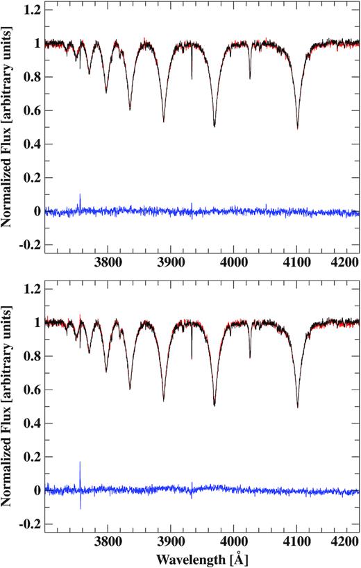
Subtraction of the XSHOOTER UVB spectrum in the secondary eclipse (black, orbital phase: 0.018) from the spectra before and after the secondary eclipse (red, orbital phases: 0.978 and 0.058). The residuals are given in blue.
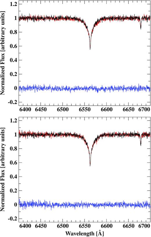
Same figure as Fig. E1, but for the VIS arm around Hα.
APPENDIX F: RADIAL VELOCITIES
Radial velocities.
| mid−BJDTBD | RV (|${\rm km\, s^{-1}}$|) | Instrument |
|---|---|---|
| |$-2\, 450\, 000$| | ||
| 3816.608090 | −12.5 ± 6.8 | SDSS† |
| 3816.622170 | −28.4 ± 6.2 | |
| 3816.637894 | −26.0 ± 7.1 | |
| 3816.653623 | 21.4 ± 6.7 | |
| 3816.669271 | 49.0 ± 10.5 | |
| 3816.684919 | 38.4 ± 8.8 | |
| 4755.79740 | 58.9 ± 15.8 | EFOSC2† |
| 4755.80127 | 45.1 ± 14.4 | |
| 4757.84839 | −40.7 ± 15.0 | |
| 4757.85225 | −35.4 ± 12.4 | |
| 5146.80965 | 47.5 ± 8.0 | |
| 5146.82778 | 59.9 ± 8.0 | |
| 5146.83743 | 47.5 ± 8.0 | |
| 5147.80109 | 19.5 ± 8.9 | |
| 5147.81597 | −14.9 ± 8.1 | |
| 5147.82562 | −34.0 ± 7.9 | |
| 5147.84031 | −29.3 ± 8.9 | |
| 5147.84997 | −6.2 ± 8.6 | |
| 5147.86465 | 34.9 ± 9.5 | |
| 5147.87430 | 49.2 ± 8.5 | |
| 5148.77113 | 4.5 ± 8.5 | |
| 5148.77964 | −20.1 ± 7.9 | |
| 5148.79388 | −38.7 ± 7.8 | |
| 5148.80354 | −37.5 ± 9.0 | |
| 5657.49252374 | 42.5 ± 5.3 | UVES |
| 5657.49654962 | 4.9 ± 3.7 | |
| 5657.50057560 | −0.9 ± 5.2 | |
| 5657.50461775 | −4.8 ± 5.6 | |
| 5657.50866197 | −9.1 ± 3.1 | |
| 5657.51270167 | −19.0 ± 4.2 | |
| 5657.51674196 | −21.5 ± 2.3 | |
| 5657.52107057 | −20.1 ± 3.0 | |
| 5657.52509622 | −17.0 ± 7.9 | |
| 5657.52912257 | −11.1 ± 6.9 | |
| 5657.53316028 | −2.5 ± 2.5 | |
| 5657.53720219 | 12.2 ± 6.8 | |
| 5657.54124410 | 22.8 ± 6.1 | |
| 5657.54528808 | 33.1 ± 6.7 | |
| 5657.54932975 | 43.2 ± 6.5 | |
| 5657.55337328 | 60.0 ± 4.5 | |
| 5657.55741668 | 60.6 ± 2.2 | |
| 5657.56145535 | 69.1 ± 7.6 | |
| 5657.56549517 | 74.9 ± 6.4 | |
| 5657.56953256 | 73.7 ± 5.2 | |
| 5657.57357041 | 78.2 ± 8.8 | |
| 5657.57760966 | 65.4 ± 6.9 | |
| 5657.58569149 | 46.0 ± 8.0 | |
| 5657.58973698 | 29.8 ± 7.4 | |
| 5657.59377830 | 13.7 ± 6.7 | |
| 5657.59782484 | −3.2 ± 5.8 | |
| 5657.60590841 | −15.8 ± 5.1 | |
| 5657.61398712 | −27.9 ± 6.5 | |
| 7801.53891733 | 61.5 ± 1.6 | XSHOOTER |
| 7801.54280358 | 52.3 ± 1.0 | |
| 7801.54661453 | 42.4 ± 0.9 | |
| 7801.55049162 | 35.6 ± 1.3 | |
| 7801.55428555 | 10.5 ± 1.2 | |
| 7801.55816729 | 6.2 ± 1.0 | |
| 7801.56197835 | −2.7 ± 1.1 | |
| 7801.56585983 | −11.2 ± 1.0 | |
| 7801.56967460 | −19.3 ± 1.1 | |
| 7801.57356027 | −22.1 ± 1.2 | |
| 7801.57736624 | −19.4 ± 0.9 | |
| 7801.58125282 | −17.1 ± 0.9 | |
| 7801.58774688 | −5.4 ± 0.9 | |
| 7801.59163370 | 5.4 ± 1.0 | |
| 7801.59543481 | 14.9 ± 1.0 | |
| 7801.59932441 | 26.3 ± 1.0 | |
| 7801.60313072 | 38.8 ± 0.8 | |
| 7801.60701615 | 47.9 ± 1.0 | |
| 7801.61081599 | 58.7 ± 1.0 | |
| 7801.61851422 | 72.3 ± 1.3 | |
| 7801.62238622 | 74.5 ± 0.9 | |
| 7801.62620191 | 74.8 ± 1.1 | |
| 7801.63009857 | 69.0 ± 1.2 |
Note:†Geier et al. (2011c).
APPENDIX G: TIMES OF PRIMARY ECLIPSES
Times of the primary eclipse of J08205+0008.
| Eclipse number | Time of primary eclipse | Source |
|---|---|---|
| [BJDTDB] | ||
| 0 | 2455165.709266 ± 0.000050 | Merope† |
| 31 | 2455168.692622 ± 0.000050 | Merope† |
| 465 | 2455210.461047 ± 0.000050 | Merope† |
| 466 | 2455210.557368 ± 0.000050 | Merope† |
| 467 | 2455210.653586 ± 0.000050 | Merope† |
| 3980 | 2455548.747324 ± 0.000020 | ULTRACAM |
| 4704 | 2455618.425621 ± 0.000050 | BUSCA |
| 4745 | 2455622.371553 ± 0.000050 | BUSCA |
| 8071 | 2455942.468130 ± 0.000050 | SAAO |
| 8072 | 2455942.564480 ± 0.000010 | SAAO |
| 11179 | 2456241.584370 ± 0.000020 | SAAO |
| 12103 | 2456330.510900 ± 0.000030 | SAAO |
| 12113 | 2456331.473260 ± 0.000020 | SAAO |
| 12164 | 2456336.381490 ± 0.000030 | SAAO |
| 12165 | 2456336.477810 ± 0.000040 | SAAO |
| 12537 | 2456372.279310 ± 0.000010 | SAAO |
| 12568 | 2456375.262750 ± 0.000080 | SAAO |
| 12973 | 2456414.240300 ± 0.000050 | SAAO |
| 13035 | 2456420.207310 ± 0.000040 | SAAO |
| 15822 | 2456688.430140 ± 0.000020 | SAAO |
| 15832 | 2456689.392530 ± 0.000050 | SAAO |
| 15863 | 2456692.376020 ± 0.000020 | SAAO |
| 16101 | 2456715.281300 ± 0.000050 | SAAO |
| 16132 | 2456718.264780 ± 0.000100 | SAAO |
| 16703 | 2456773.218230 ± 0.000050 | SAAO |
| 16724 | 2456775.239280 ± 0.000030 | SAAO |
| 18567 | 2456952.610940 ± 0.000020 | SAAO |
| 19459 | 2457038.457650 ± 0.000020 | SAAO |
| 19470 | 2457039.516330 ± 0.000030 | SAAO |
| 19490 | 2457041.441110 ± 0.000030 | SAAO |
| 19739 | 2457065.405120 ± 0.000030 | SAAO |
| 19780 | 2457069.350940 ± 0.000040 | SAAO |
| 20413 | 2457130.271420 ± 0.000030 | SAAO |
| 20444 | 2457133.254870 ± 0.000020 | SAAO |
| 20714 | 2457159.239800 ± 0.000030 | SAAO |
| 20724 | 2457160.202340 ± 0.000030 | SAAO |
| 23179 | 2457396.473170 ± 0.000080 | SAAO |
| 23210 | 2457399.456640 ± 0.000030 | SAAO |
| 23459 | 2457423.420580 ± 0.000010 | SAAO |
| 23490 | 2457426.404090 ± 0.000020 | SAAO |
| 27710 | 2457832.53995 ± 0.000020 | ULTRACAM |
| 28330 | 2457892.209190 ± 0.000050 | SAAO |
| 31179 | 2458166.399050 ± 0.000080 | SAAO |
| 31480 | 2458195.367510 ± 0.000030 | SAAO |
| 34868 | 2458521.431060 ± 0.000030 | SAAO |
| 35469 | 2458579.271780 ± 0.000030 | SAAO |
| 37872 | 2458810.538190 ± 0.000030 | SAAO |
| 37883 | 2458811.596860 ± 0.000030 | SAAO |
| 37893 | 2458812.559230 ± 0.000030 | SAAO |
| 39034 | 2458922.369960 ± 0.000010 | SAAO |
| 39117 | 2458930.357940 ± 0.000030 | SAAO |
Note:†Geier et al. (2011c).
