Analysis of eclipsing binaries in multiple stellar systems: the case of V1200 Centauri

Marcadon, F; Hełminiak, K G; Marques, J P; Pawłaszek, R; Sybilski, P; Kozłowski, S K; Ratajczak, M; Konacki, M

doi:10.1093/mnras/staa3040

ABSTRACT

We present a new analysis of the multiple-star V1200 Centauri based on the most recent observations for this system. We used the photometric observations from the Solaris network and the Transiting Exoplanet Survey Satellite telescope, combined with the new radial velocities from the CHIRON spectrograph and those published in the literature. We confirmed that V1200 Cen consists of a 2.5-d eclipsing binary orbited by a third body. We derived the parameters of the eclipsing components, which are |$M_{\mathrm{ Aa}} = 1.393\pm 0.018\,$|M_⊙, |$R_{\mathrm{ Aa}} = 1.407\pm 0.014\,$|R_⊙, and |$T_{{\rm eff},\mathrm{ Aa}} = 6588\pm 58\,$|K for the primary, and |$M_{\mathrm{ Ab}} = 0.8633\pm 0.0081\,$|M_⊙, |$R_{\mathrm{ Ab}} = 1.154\pm 0.014\,$|R_⊙, and |$T_{{\rm eff},\mathrm{ Ab}} = 4475\pm 68\,$|K for the secondary. Regarding the third body, we obtained significantly different results than those previously published. The period of the outer orbit is found to be 180.4 d, implying a minimum mass of |$M_\mathrm{ B} = 0.871\pm 0.020\,$|M_⊙. Thus, we argue that V1200 Cen is a quadruple system with a secondary pair composed of two low-mass stars. Finally, we determined the ages of each eclipsing component using two evolution codes, namely mesa and cestam. We obtained ages of 16–18.5 and 5.5–7 Myr for the primary and the secondary, respectively. In particular, the secondary appears larger and hotter than that predicted at the age of the primary. We concluded that dynamical and tidal interactions occurring in multiples may alter the stellar properties and explain the apparent non-coevality of V1200 Centauri.

binaries: eclipsing, binaries: spectroscopic, stars: fundamental parameters, stars: individual: V1200 Cen

1 INTRODUCTION

Binary or multiple stellar systems are very common in our Galaxy. Over the past century, stellar duplicity has been reported using different techniques from ground- and space-based instruments (e.g. spectroscopy, interferometry, and photometry). Depending on the nature of the observations, these systems are referred to as spectroscopic, visual, eclipsing, or astrometric binaries. More recently, asteroseismology has allowed the discovery of binary stars showing solar-like oscillations in both components of the system, that is seismic binaries (see e.g. Marcadon, Appourchaux & Marques 2018, for a review). For such systems, a model-dependent approach is required to determine their stellar parameters. In this context, eclipsing binaries (EBs) that are also double-lined spectroscopic binaries provide a direct determination of the stellar parameters through their dynamics. The stellar masses and radii can then be measured with exquisite precision below ∼1–3|${{\ \rm per\ cent}}$| (Torres, Andersen & Giménez 2010). Precise stellar parameters are actually crucial for calibrating theoretical models of stars, mainly during the pre-main-sequence (PMS) phase, where evolution is more rapid.

EBs with low-mass PMS stars represent a real challenge for theoretical models due to the complexity of the stellar physics involved (Stassun, Feiden & Torres 2014). These kinds of systems are therefore valuable test cases for models at early stages of stellar evolution. Unfortunately, there are only few systems with such features reported in the literature. Gómez Maqueo Chew et al. (2019) listed 14 known EBs with masses, radii, and ages below 1.4|$\, {\rm M}_\odot$|⁠, 2.4|$\, {\rm R}_\odot$|⁠, and 17 Myr, respectively (see references therein). Another system was identified as a possible candidate by Coronado et al. (2015), namely V1200 Centauri. However, the precision on the derived parameters, in particular stellar radii, did not allow the authors to properly determine the individual ages of the eclipsing components (⁠|${\sim} 30\,$|Myr). In this work, we propose to re-analyse V1200 Cen using the most recent observations of the system. From their radial-velocity (RV) analysis, Coronado et al. (2015) claimed that V1200 Cen is a hierarchical triple-star system with an outer period of almost 1 yr. Here, we argue that the third body is itself a binary system, making V1200 Cen a quadruple-star system with a 180-d outer period.

Due to its multiplicity, V1200 Cen appears to be an interesting target for studying the dynamical evolution of multiple-star systems. In particular, the dynamics of hierarchical quadruple systems is a difficult problem that has been investigated by a number of authors (see Hamers 2019, and references therein). For triple and quadruple systems, it has notably been shown that the period distributions of inner orbits present an enhancement at a few to several tens of days (Tokovinin 2008). In the case of triple systems, the formation of a short-period binary can be explained by Lidov–Kozai (Kozai 1962; Lidov 1962) cycles with tidal friction (see e.g. Toonen, Hamers & Portegies Zwart 2016, for a review). A legitimate question is whether this mechanism extends to quadruple-star systems, especially for those with PMS stars in a close orbit. Hamers (2019) suggested that others processes occurring during the stellar formation may produce such quadruple systems with close inner pairs. It is widely accepted that stars belonging to a binary or multiple system are formed at the same time from the same interstellar material (Tohline 2002). However, this hypothesis needs to be tested in the case of specific systems such as V1200 Cen.

This article is organized as follows: Section 2 describes the observational data used in this work, including Solaris and Transiting Exoplanet Survey Satellite (TESS) photometry as well as RV measurements of V1200 Cen. Section 3 presents the light-curve and RV analysis of the system leading to the determination of the stellar masses and radii for the two eclipsing components. In Section 4, we discuss the implications of the main features of V1200 Cen on its evolutionary status. Finally, the conclusions of this work are summarized in Section 5.

2 OBSERVATIONS

2.1 Solaris photometry

We collected photometric data for V1200 Cen during three main campaigns of observation between 2017 February and August (∼75 nights), between 2018 March and August (∼55 nights), and between 2019 February and April (∼25 nights) with Solaris, a network of four autonomous observatories in the Southern hemisphere (Kozłowski et al. 2014, 2017). The Solaris network aims to detect exoplanets around binaries and multiple stars such as V1200 Cen using high-cadence and high-precision photometric observations of these systems (Konacki et al. 2012). This global network allows a continuous night-time coverage from the end of March until mid-September due to the location of the four stations: Solaris-1 and Solaris-2 in the South African Astronomical Observatory¹ in South Africa, Solaris-3 in Siding Spring Observatory² in Australia, and Solaris-4 in Complejo Astronómico El Leoncito³ in Argentina. Each station is equipped with a 0.5-m diameter reflecting telescope. Solaris-3 is a Schmidt–Cassegrain f/9 optical system equipped with a field corrector whereas the other telescopes are Ritchey–Chrétien f/15 optical systems. All four telescopes utilize Andor iKon-L CCD cameras thermoelectrically cooled to −70^○ Celsius during observations.

Solaris telescopes allow multicolour photometry in 10 bands using Johnson (UBVRI) and Sloan (u^′g^′r^′i^′z^′) filters. Following the work of Coronado et al. (2015) on V1200 Cen, we observed this system both in the V and I bands in order to obtain a better signal-to-noise ratio in the infrared for the secondary eclipse. The image acquisition process of Solaris is described in detail in Kozłowski et al. (2017; their fig. 13) and includes the typical calibration steps, i.e. bias and dark frame acquisition as well as flat-fielding for all the different filters considered. For the data reduction, we adopted a custom photometric pipeline based on the Photutils⁴ package of Astropy (Bradley et al. 2019). Each raw science image was then bias subtracted and corrected for CCD inhomogeneities using dedicated flat-field frames. In this work, we employed the differential photometry method in order to limit the variability of the signal due to atmospheric conditions. As comparison star, we used the closer and brightest target around V1200 Cen in the Solaris field of view (13–21 arcmin), namely TYC 7790-1580-1. This latter has a V magnitude of 10.632 (Munari et al. 2014). Aperture photometry was performed by defining fixed star apertures and sky background annulus for both the target and the comparison star.

Finally, we applied the Wōtan⁵ detrending algorithm developed by Hippke et al. (2019) to the light curves obtained from our photometric pipeline. Among the proposed methods, we adopted a sum-of-(co)sines approach associated with an iterative sigma-clipping technique. In order to avoid distortions in the eclipse profiles, Wōtan offers the possibility of masking them during detrending. However, at the time of writing, this feature was implemented only for the sum-of-(co)sines approach in Wōtan. The final light curves were then obtained by applying the Wōtan detrending algorithm with two filters of different widths. Indeed, we took into account both the long-term variability of the comparison star using a 2-d filter and the short-term atmospheric fluctuations using a 2-h filter. The resulting light curves consist in total of |${\sim} 30\, 000$| data points in V and I, respectively.

2.2 TESS photometry

V1200 Cen was observed by the TESS (Ricker et al. 2015) in 2-min cadence mode for 27.1 d during sector 11,⁶ that is between 2019 April 23 and 2019 May 20. In this work, we analysed the high-precision photometric data collected by TESS for V1200 Cen (TIC 166624433), in addition to the Solaris light curves. These data were generated by the TESS Science Processing Operations Center (Jenkins et al. 2016) and made available on the Mikulski Archive for Space Telescopes (MAST).⁷ In particular, we used the Pre-search Data Conditioning Simple Aperture Photometry (PDCSAP; Smith et al. 2012; Stumpe et al. 2012, 2014) version of the light curve, which has been corrected for instrumental effects and contamination by nearby stars. As seen in Fig. 1, there are five additional stars identified as TESS targets within the optimal aperture used to extract the light curve of V1200 Cen: TIC 166624435, TIC 166624434, TIC 166624431, TIC 166624443, and TIC 166624426. Their corresponding magnitudes in the TESS band are 16.56, 18.18, 17.07, 17.50, and 18.15 mag, respectively. Given that V1200 Cen has a TESS magnitude of 7.93 mag, we estimated the contribution of the contaminant stars to the total flux measured by TESS to be lower than 0.1 per cent. Fig. 2 shows the comparison between the SAP and PDCSAP light curves of V1200 Cen.

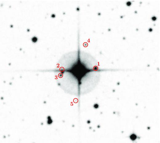
$A $4 \times 4\,$arcmin2 image centred on V1200 Cen. The five stars shown by open red circles are located within the optimal aperture as defined in the Data Validation (DV) Report for V1200 Cen. For these five stars, the contribution to the total flux is very small (<0.1 per cent). There are three other stars (not outlined in the picture) that lie within the optimal aperture. However, even taking them into account, the flux excess due to contaminant stars will not be larger than about 0.2–0.3 per cent.$

Figure 1.

A |$4 \times 4\,$|arcmin² image centred on V1200 Cen. The five stars shown by open red circles are located within the optimal aperture as defined in the Data Validation (DV) Report for V1200 Cen. For these five stars, the contribution to the total flux is very small (<0.1 per cent). There are three other stars (not outlined in the picture) that lie within the optimal aperture. However, even taking them into account, the flux excess due to contaminant stars will not be larger than about 0.2–0.3 per cent.

Open in new tab Download slide

Figure 2.

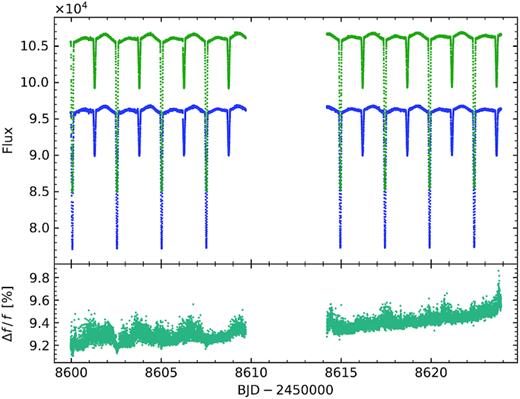
SAP (blue) and PDCSAP (green) light curves of V1200 Cen. The relative flux difference is plotted in the lower panel. The linear trend seen in the flux difference was taken into account when fitting the SAP and PDCSAP light curves. Furthermore, the variability of the flux difference does not exceed 0.2 per cent.

Open in new tab Download slide

The TESS observations of sector 11 correspond to orbits 29 and 30 of the spacecraft around the Earth. At the start of both orbits, camera 1 that observed V1200 Cen was disabled due to strong scattered light signals affecting the systematic error removal in PDC.⁸ A consequence is the presence of two gaps in the time series, which contains |$13\, 887$| flux measurements, implying a degraded duty cycle of |${\sim} 71{{\ \rm per\ cent}}$|⁠. Despite this, the orbital period of the eclipsing pair, namely ∼2.5 d, is short enough to distinguish a total of 16 eclipse events in the TESS light curve (8 primary and 8 secondary). For each measurement, we converted the flux f into magnitude using the simple relation |$m = -2.5\log(f/\tilde{f})+m_T$|, where |$\tilde{f}$| corresponds to the median flux value in the out-of-eclipse portions of the light curve and |$m_\mathrm{ T} = 7.93\,$|mag is the TESS magnitude of V1200 Cen.

2.3 New spectroscopy

In this work, we utilize the data gathered by Coronado et al. (2015), who calculated radial velocities of V1200 Cen from spectra taken with PUCHEROS and CORALIE spectrographs. However, in order to refine the parameters of the system, and better constrain the outer orbit, we made additional spectroscopic observations of V1200 Cen with the CHIRON instrument (Schwab et al. 2012; Tokovinin et al. 2013), attached to the 1.5-m telescope of the SMARTS consortium, located in the Cerro Tololo Inter-American Observatory (CTIO) in Chile. We monitored the target between 2019 May and September, taking six spectra in the ‘fibre’ mode, which provides high efficiency and spectral resolution of R ≃ 28 000. The exposure time was set to 600 s for the first four observations and 867 s for the remaining two. The resulting signal-to-noise ratio S/N varied between 110 and 170, with the exception of the fourth spectrum (S/N ≃ 25). We aimed for the S/N higher than that in previous PUCHEROS and CORALIE observations in order to search for signatures of the third body, but we have found nothing conclusive (see Section 3.4).

Data reduction and spectra extraction were performed onsite with the dedicated pipeline (Tokovinin et al. 2013), and barycentric corrections to time and velocity were calculated with the bcvcor task of the rvsao package under iraf. The RVs were calculated with our own implementation of the TODCOR method (Mazeh & Zucker 1994), for which we used two synthetic ATLAS9 template spectra: T_eff = 6300 K, v_rot = 25 km s⁻¹ for the primary, and T_eff = 4700 K, v_rot = 20 km s⁻¹ for the secondary. Measurement errors were estimated with a bootstrap procedure (Hełminiak et al. 2012), sensitive to S/N and rotational broadening of spectral lines.

3 ANALYSIS

3.1 Light-curve modelling

For the light-curve analysis of the TESS and Solaris data, we used the latest version (v34) of the jktebop ⁹ code (Southworth, Maxted & Smalley 2004a; Southworth et al. 2004b), which is based on the Eclipsing Binary Orbit Program (ebop; Popper & Etzel 1981). We chose to fit the TESS and Solaris light curves using the same code as Coronado et al. (2015) in order to compare and combine the results from different surveys. Although the current version of jktebop allows for fitting both the light curve and the RV curves simultaneously, we did not use the RV data for the modelling. Indeed, the RV modulation of the eclipsing pair by a third body cannot be reproduced using the version 34 of jktebop. Moreover, the code is not designed to fit multiband light curves. In this model, the components are approximated as biaxial spheroids for the calculation of the reflection and ellipsoidal effects, and as spheres for the eclipse shapes. In addition, the jktebop code implements a Levenberg–Marquardt minimization method that allows us to find the best-fitting model parameters, including period P, time of primary minimum T₀, eccentricity e, argument of periastron ω, inclination i, central surface brightness ratio J, sum of the fractional radii r₁ + r₂ (in units of semimajor axis a), and their ratio k = r₂/r₁. We also fitted the limb-darkening (LD) coefficients by adopting the logarithmic LD law proposed by Klinglesmith & Sobieski (1970). Initial values of the LD coefficients were taken from the tables of van Hamme (1993). We did not find evidence of a third light during the preliminary analysis of the TESS and Solaris data. As a result, the term l₃/l_tot was kept equal to zero when fitting the light curves.

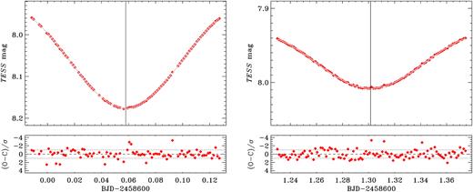
First, using jktebop, we performed the LC modelling of the high-precision TESS photometric data. In addition to the model prescriptions detailed above, we also fitted the linear trend observed in the PDCSAP light curve as well as three sinusoidal curves with respective periods of ∼P, ∼P/2, and ∼P/3. For both the SAP and PDCSAP light curves, we identified the frequencies corresponding to ∼P, ∼P/2, and ∼P/3 in the Lomb–Scargle periodogram (Lomb 1976; Scargle 1982). We performed an initial fit of the light curves without sinusoidal modulation. Three sine waves with periods derived from the periodogram were then added, one by one, to the light curves. This allows us to take the contribution of stellar activity, such as spots, into account. In this way, periodic variations with a semi-amplitude higher than about 0.7 mmag were removed from the TESS light curve, which is shown in Fig. 3. For each model, we checked that the derived parameters are still consistent within their error bars. In contrast to the previous analysis of Coronado et al. (2015), the orbital eccentricity was found to be slightly different from zero. Indeed, a value of e = 0.01 is required to properly fit the high-precision TESS light curve. We then kept the eccentricity fixed to this value when modelling the Solaris light curves. Furthermore, using TESS photometry, we reduced by a factor of ∼7 the uncertainty on the orbital inclination such as derived by Coronado et al. (2015). This can be seen in Fig. 4 where we plotted the distribution of the inclination as a function of r₁ + r₂ and k (for a comparison, see fig. 3 of Coronado et al. 2015). Again, we adopted the value derived from TESS photometry, i = 81.38^○ ± 0.18^○, as a fixed parameter in the model fitting of the Solaris light curves. In Fig. 3, we presented the observed TESS and Solaris light curves associated with their best-fitting models derived from our analysis. The root mean squares (rms) of the residuals are |$0.6$| and |$12.0\,$|mmag, respectively.

Figure 3.

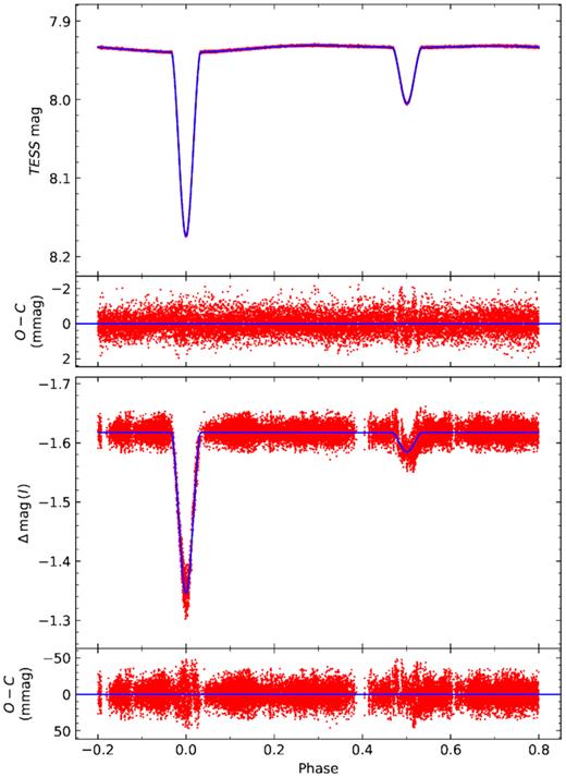
Phase-folded light curves of V1200 Cen from TESS (top) and Solaris in theI band (bottom). Red dots denote the observations while the blue line corresponds to the best-fitting model obtained with jktebop. Fitting residuals are shown in lower panels. The I-band light curve was detrended before fitting in order to remove the long-term variability of the comparison star and the short-term atmospheric fluctuations. We used a detrending algorithm, namely Wōtan, which offers the possibility of masking the eclipses during the procedure. For the TESS light curve, we proceeded in the way described in Section 3.1. For graphical clarity, we removed the linear trend and the three sine waves from the TESS data before plotting them.

Open in new tab Download slide

Figure 4.

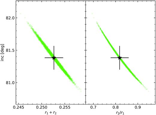
Results of the Monte Carlo analysis performed with jktebop on the TESS data. Both plots present the distribution of the best-fitting models in the i versus r₁ + r₂ (left) and i versus k = r₂/r₁ (right) planes. Black stars with error bars indicate the mean values of the different parameters with their corresponding 1σ uncertainties.

Open in new tab Download slide

In order to derive reliable uncertainties, we performed Monte Carlo simulations on the TESS and Solaris light curves, with |$10\, 000$| runs each, as implemented in jktebop (Southworth et al. 2005). For the Solaris light curves, the model parameters that were held fixed during the fitting procedure, i.e. e and i, were then perturbed in the Monte Carlo error analysis. Thus, the correlation between the fitted parameters can be assessed (see Fig. 4). In Table 1, we summarized the results derived in this work, as well as those obtained by Coronado et al. (2015) from the All-Sky Automated Survey (ASAS; Pojmanski 2002; Paczyński et al. 2006) and Wide Angle Search for Planets (SuperWASP; Pollacco et al. 2006) surveys. We obtained very consistent results between the four surveys, based on various approaches. The main difference concerns the fractional radius of the secondary star, r₂, for which our estimate is about |$4{{\ \rm per\ cent}}$| higher than the value adopted by Coronado et al. (2015). This is consistent with the correlations shown in Fig. 4, where a lower inclination implies larger values of r₁ + r₂ and k, and thus a larger fractional secondary radius. Thanks to the high precision of the TESS photometry, we also significantly improved the precision on the fractional radii (⁠|${\sim }1{{\ \rm per\ cent}}$|⁠). From the fit of the SAP light curve, adopting the same approach as for the PDCSAP light curve, we obtained consistent results within their error bars, i.e. |$r_1 = 0.137\, 9\pm 0.002\, 9$|⁠, |$r_2 = 0.116\, 1\pm 0.005\, 6$|⁠, and i = 81.27^○ ± 0.25^○. Thus, the use of either the SAP or PDCSAP light curves does not change our conclusions. The implications of these results will be discussed in detail in Section 4.

Table 1.

Open in new tab

Parameters obtained from our analysis of the TESS and Solaris light curves and from the previous analysis of the ASAS and SuperWASP (SW) light curves by Coronado et al. (2015). The Solaris values correspond to the I-band light curve shown in Fig. 3. The values without error bars were held fixed during the fitting procedure. The adopted values are weighted means.

Parameter	TESS value	Solaris value	ASAS value	SW value	Adopted value
P (d)	2.482 7327(69)	2.482 9615(44)	2.482 8778(43)	2.482 8752(25)	2.482 8811(19)
T₀ (JD\|$-245\,0000$\|⁠)	1883.864 432(39)	1883.860 791(91)	1883.8789(31)	1883.8827(24)	1883.863 863(36)
T (JD\|$-245\,0000$\|⁠)	1883.807 765(39)	1883.804 266(91)	1883.8789(31)	1883.8827(24)	1883.807 212(36)^a
e	0.010 1080(25)	0.010 1080	0	0	0.010 1080(25)^b
i (^○)	81.38\|$\, \pm \,$\|0.18	81.38	81.9\|$^{+2.8}_{-1.3}$\|	81.6\|$^{+1.6}_{-1.3}$\|	81.38\|$\, \pm \, 0.18^{\it b}$\|
r₁	0.1389\|$\, \pm \,$\|0.0019	0.1391\|$\, \pm \,$\|0.0018	0.137\|$^{+0.014}_{-0.015}$\|	0.138\|$^{+0.025}_{-0.034}$\|	0.1390\|$\, \pm \,$\|0.0013
r₂	0.1137\|$\, \pm \,$\|0.0038	0.1141\|$\, \pm \,$\|0.0014	0.107\|$^{+0.024}_{-0.039}$\|	0.110\|$^{+0.038}_{-0.026}$\|	0.1140\|$\, \pm \,$\|0.0013^c

Parameter	TESS value	Solaris value	ASAS value	SW value	Adopted value
P (d)	2.482 7327(69)	2.482 9615(44)	2.482 8778(43)	2.482 8752(25)	2.482 8811(19)
T₀ (JD\|$-245\,0000$\|⁠)	1883.864 432(39)	1883.860 791(91)	1883.8789(31)	1883.8827(24)	1883.863 863(36)
T (JD\|$-245\,0000$\|⁠)	1883.807 765(39)	1883.804 266(91)	1883.8789(31)	1883.8827(24)	1883.807 212(36)^a
e	0.010 1080(25)	0.010 1080	0	0	0.010 1080(25)^b
i (^○)	81.38\|$\, \pm \,$\|0.18	81.38	81.9\|$^{+2.8}_{-1.3}$\|	81.6\|$^{+1.6}_{-1.3}$\|	81.38\|$\, \pm \, 0.18^{\it b}$\|
r₁	0.1389\|$\, \pm \,$\|0.0019	0.1391\|$\, \pm \,$\|0.0018	0.137\|$^{+0.014}_{-0.015}$\|	0.138\|$^{+0.025}_{-0.034}$\|	0.1390\|$\, \pm \,$\|0.0013
r₂	0.1137\|$\, \pm \,$\|0.0038	0.1141\|$\, \pm \,$\|0.0014	0.107\|$^{+0.024}_{-0.039}$\|	0.110\|$^{+0.038}_{-0.026}$\|	0.1140\|$\, \pm \,$\|0.0013^c

Notes. ^aThe term T corresponds to the time of periastron passage, which is different to the time of primary minimum T₀ when e ≠ 0. The adopted value of T was thus computed as the weighted mean of only the TESS and Solaris values. The values were shifted by |$n\bar{P}$|⁠, where n is an integer and |$\bar{P}$| corresponds to the mean period derived from the different surveys.

^bFor e and i, we adopted the well-constrained values from TESS.

^cThe adopted value of r₂ was computed as the weighted mean of the TESS and Solaris values (see the text).

Table 1.

Open in new tab

Parameters obtained from our analysis of the TESS and Solaris light curves and from the previous analysis of the ASAS and SuperWASP (SW) light curves by Coronado et al. (2015). The Solaris values correspond to the I-band light curve shown in Fig. 3. The values without error bars were held fixed during the fitting procedure. The adopted values are weighted means.

Parameter	TESS value	Solaris value	ASAS value	SW value	Adopted value
P (d)	2.482 7327(69)	2.482 9615(44)	2.482 8778(43)	2.482 8752(25)	2.482 8811(19)
T₀ (JD\|$-245\,0000$\|⁠)	1883.864 432(39)	1883.860 791(91)	1883.8789(31)	1883.8827(24)	1883.863 863(36)
T (JD\|$-245\,0000$\|⁠)	1883.807 765(39)	1883.804 266(91)	1883.8789(31)	1883.8827(24)	1883.807 212(36)^a
e	0.010 1080(25)	0.010 1080	0	0	0.010 1080(25)^b
i (^○)	81.38\|$\, \pm \,$\|0.18	81.38	81.9\|$^{+2.8}_{-1.3}$\|	81.6\|$^{+1.6}_{-1.3}$\|	81.38\|$\, \pm \, 0.18^{\it b}$\|
r₁	0.1389\|$\, \pm \,$\|0.0019	0.1391\|$\, \pm \,$\|0.0018	0.137\|$^{+0.014}_{-0.015}$\|	0.138\|$^{+0.025}_{-0.034}$\|	0.1390\|$\, \pm \,$\|0.0013
r₂	0.1137\|$\, \pm \,$\|0.0038	0.1141\|$\, \pm \,$\|0.0014	0.107\|$^{+0.024}_{-0.039}$\|	0.110\|$^{+0.038}_{-0.026}$\|	0.1140\|$\, \pm \,$\|0.0013^c

Parameter	TESS value	Solaris value	ASAS value	SW value	Adopted value
P (d)	2.482 7327(69)	2.482 9615(44)	2.482 8778(43)	2.482 8752(25)	2.482 8811(19)
T₀ (JD\|$-245\,0000$\|⁠)	1883.864 432(39)	1883.860 791(91)	1883.8789(31)	1883.8827(24)	1883.863 863(36)
T (JD\|$-245\,0000$\|⁠)	1883.807 765(39)	1883.804 266(91)	1883.8789(31)	1883.8827(24)	1883.807 212(36)^a
e	0.010 1080(25)	0.010 1080	0	0	0.010 1080(25)^b
i (^○)	81.38\|$\, \pm \,$\|0.18	81.38	81.9\|$^{+2.8}_{-1.3}$\|	81.6\|$^{+1.6}_{-1.3}$\|	81.38\|$\, \pm \, 0.18^{\it b}$\|
r₁	0.1389\|$\, \pm \,$\|0.0019	0.1391\|$\, \pm \,$\|0.0018	0.137\|$^{+0.014}_{-0.015}$\|	0.138\|$^{+0.025}_{-0.034}$\|	0.1390\|$\, \pm \,$\|0.0013
r₂	0.1137\|$\, \pm \,$\|0.0038	0.1141\|$\, \pm \,$\|0.0014	0.107\|$^{+0.024}_{-0.039}$\|	0.110\|$^{+0.038}_{-0.026}$\|	0.1140\|$\, \pm \,$\|0.0013^c

Notes. ^aThe term T corresponds to the time of periastron passage, which is different to the time of primary minimum T₀ when e ≠ 0. The adopted value of T was thus computed as the weighted mean of only the TESS and Solaris values. The values were shifted by |$n\bar{P}$|⁠, where n is an integer and |$\bar{P}$| corresponds to the mean period derived from the different surveys.

^bFor e and i, we adopted the well-constrained values from TESS.

^cThe adopted value of r₂ was computed as the weighted mean of the TESS and Solaris values (see the text).

3.2 Radial velocities and spectroscopic orbit

In this section, we present the methodology employed to process the RV measurements of V1200 Cen. Our analysis is based on the previously published RVs from the PUCHEROS¹⁰ and CORALIE¹¹ spectrographs (Coronado et al. 2015), supplemented by our own measurements collected with CHIRON (see Section 2.3). All previous and new RV measurements are provided in Table A1 in the appendix.

Recently, Marcadon et al. (2018) derived the orbit of the Kepler target HD 188753 by applying a Bayesian analysis to the astrometric and RV measurements of the system. We adapted this Bayesian approach in order to fit a double-Keplerian orbit using the available RV data for V1200 Cen. Thus, we defined the likelihood of the RV data given the orbital parameters as

$$\begin{eqnarray*} \ln {\cal L}_{\rm RV} = -\frac{1}{2}\, \sum ^{N_{\rm RV}}_{i=1} \, \left(\frac{V_i^{\rm mod}-V_i^{\rm obs}}{\sigma _{V,i}} \right)^2, \end{eqnarray*}$$

(1)

where N_RV denotes the number of observed radial velocities (V^obs) and σ_V refers to the associated uncertainties. Here, the term V^mod corresponds to the RV values computed using an adapted version of the observable model described in Marcadon et al. (2018). This new version takes into account the third-body perturbation by considering the orbital parameters |$\mathcal {P}_{\rm orb} = (K_{\mathrm{ Aa}},K_{\mathrm{ Ab}},P_\mathrm{ A},T_\mathrm{ A},e_\mathrm{ A},\omega _\mathrm{ A},K_{\mathrm{ A}},P_{\mathrm{ AB}},T_{\mathrm{ AB}},e_{\mathrm{ AB}},\omega _{\mathrm{ AB}},\gamma _{\mathrm{ AB}})$|⁠, where subscripts Aa and Ab refer, respectively, to the primary and secondary components and subscript AB refers to the relative orbit between the eclipsing pair A and the third body B. We use this notation from now on, which is more adequate to describe a possible quadruple-star system. For the derivation of these orbital parameters, we employed a Markov chain Monte Carlo (MCMC) method using the Metropolis–Hastings algorithm (Metropolis et al. 1953; Hastings 1970) as explained in Marcadon et al. (2018). Briefly, the procedure consists of setting 10 chains of 10 million points each with starting points taken randomly from appropriate distributions. The new set of orbital parameters is here computed using a random walk as follows:

$$\begin{eqnarray*} {\cal P}_{\rm orb}^{t^{\prime }}={\cal P}_{\rm orb}^{t}+\alpha _{\rm rate} \, \Delta {\cal P}_{\rm orb}, \end{eqnarray*}$$

(2)

where |$\Delta {\cal P}_{\rm orb}$| is given by a multinomial normal distribution with independent parameters and α_rate is an adjustable parameter that is reduced by a factor of 2 until the rate of acceptance of the new set exceeds 25|${{\ \rm per\ cent}}$|⁠. We then derived the posterior probability of each parameter from the chains after rejecting the initial burn-in phase (i.e. the first 10|${{\ \rm per\ cent}}$| of each chain). For all parameters, we computed the median and the credible intervals at 16|${{\ \rm per\ cent}}$| and 84|${{\ \rm per\ cent}}$|⁠, corresponding to a 1σ interval for a normal distribution. An essential aspect when fitting data from different instruments is the determination of a proper relative weighting. To this end, we performed a preliminary set of fits and calculated the rms of the residuals for stars Aa and Ab. We obtained rms values of 0.76 and 1.80 km s⁻¹, respectively, which were adopted as weights for the final fit. We then checked that the rms values from our best solution are equal to the weights used during the fitting procedure.

Finally, the best-fitting RV solution for the whole system is shown in Fig. 5. We also indicated the corresponding orbital parameters derived from our Bayesian analysis of the RV data in Table 2. We fitted two additional terms to take into account the zero-point differences, i.e. E/C−5/P and C/C−5/P. Here, we assumed that the shift is the same for the two stars. We then obtained E/C−5/P = −0.23 ± 0.67 km s⁻¹ and C/C−5/P = −0.27 ± 0.73 km s⁻¹. The new values of the orbital and physical parameters are, within the error bars, in agreement with those presented in Table 2. Therefore, in the following, we adopted as reference the solution where E/C−5/P and C/C−5/P are equal to zero. Thanks to the new RV measurements from CHIRON, we obtained a more precise and robust solution than that of Coronado et al. (2015). Indeed, we found that the AB system has a 180-d orbital period and is almost circular with an eccentricity of 0.088. For comparison, Coronado et al. (2015) derived an orbital period of 351.5 d and an eccentricity of 0.42 for the AB system. Such a difference is due to the fact that the authors did not have enough RV data points to uniformly cover the orbit of the AB system due to uneven sampling, while the time span of our CHIRON observations is comparable to P_AB, and sampling was relatively regular. The new orbit implies a more massive third body than in the previous study, namely |$M_\mathrm{ B} = 0.871\, {\rm M}_\odot$| instead of 0.662|$\, {\rm M}_\odot$| (minimum mass for the third body, corresponding to i_AB = 90^○), whose implications will be further discussed in Section 4.

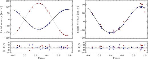
$RV curves of V1200 Cen described by a double-Keplerian orbital model using radial velocities of stars Aa (blue) and Ab (red). Upper-left panel: Best-fitting solutions for stars Aa (black) and Ab (grey) after having removed the 180-d modulation induced by the third body. The curve is phase folded at the orbital period $P_\mathrm{ A}\!\simeq 2.5\,$d, where phase 0 is set for the time of primary minimum T0. Upper-right panel: Best-fitting solution for the centre of mass of the eclipsing pair after having removed the orbital motion of stars Aa and Ab. The curve is phase folded at the orbital period $P_{\mathrm{ AB}}\!\simeq 180\,$d, where phase 0 is set for the time of periastron passage TAB. Lower panels: Residuals of the fitting procedure.$

Figure 5.

RV curves of V1200 Cen described by a double-Keplerian orbital model using radial velocities of stars Aa (blue) and Ab (red). Upper-left panel: Best-fitting solutions for stars Aa (black) and Ab (grey) after having removed the 180-d modulation induced by the third body. The curve is phase folded at the orbital period |$P_\mathrm{ A}\!\simeq 2.5\,$|d, where phase 0 is set for the time of primary minimum T₀. Upper-right panel: Best-fitting solution for the centre of mass of the eclipsing pair after having removed the orbital motion of stars Aa and Ab. The curve is phase folded at the orbital period |$P_{\mathrm{ AB}}\!\simeq 180\,$|d, where phase 0 is set for the time of periastron passage T_AB. Lower panels: Residuals of the fitting procedure.

Open in new tab Download slide

Table 2.

Open in new tab

Orbital parameters and derived quantities for the best-fitting model of the RV data.

Parameter	Median	84 per cent interval	16 per cent interval
K_Aa (km s⁻¹)	78.02	+0.28	−0.28
K_Ab (km s⁻¹)	125.89	+0.70	−0.71
P_A (d)	2.482 8811^a	±0.000 0019
T_A (JD\|$-245\,0000$\|⁠)	1883.807 212^a	±0.000 036
e_A	0.010 1080^a	±0.000 0025
ω_A (^○)	81.616^a	±0.096
K_A (km s⁻¹)	15.41	+0.27	−0.27
P_AB (d)	180.374	+0.093	−0.094
T_AB (JD\|$-245\,0000$\|⁠)	5818.7	+7.1	−6.8
e_AB	0.088	+0.018	−0.019
ω_AB (^○)	32	+13	−13
γ_AB (km s⁻¹)	1.16	+0.22	−0.22
a_Aabsin i_A (R_⊙)^b	10.006	+0.037	−0.037
q	0.6197	+0.0042	−0.0042
M_Aasin ³i_A (M_⊙)	1.346	+0.017	−0.017
M_Absin ³i_A (M_⊙)	0.8344	+0.0078	−0.0078
a_Asin i_AB (au)^b	0.2544	+0.0044	−0.0045
f(M_B) (M_⊙)	0.0675	+0.0036	−0.0035
\|$M_\mathrm{ B} \, (i_{\mathrm{ AB}}\!=90^\circ$\|⁠) (M_⊙)	0.871	+0.020	−0.020

Parameter	Median	84 per cent interval	16 per cent interval
K_Aa (km s⁻¹)	78.02	+0.28	−0.28
K_Ab (km s⁻¹)	125.89	+0.70	−0.71
P_A (d)	2.482 8811^a	±0.000 0019
T_A (JD\|$-245\,0000$\|⁠)	1883.807 212^a	±0.000 036
e_A	0.010 1080^a	±0.000 0025
ω_A (^○)	81.616^a	±0.096
K_A (km s⁻¹)	15.41	+0.27	−0.27
P_AB (d)	180.374	+0.093	−0.094
T_AB (JD\|$-245\,0000$\|⁠)	5818.7	+7.1	−6.8
e_AB	0.088	+0.018	−0.019
ω_AB (^○)	32	+13	−13
γ_AB (km s⁻¹)	1.16	+0.22	−0.22
a_Aabsin i_A (R_⊙)^b	10.006	+0.037	−0.037
q	0.6197	+0.0042	−0.0042
M_Aasin ³i_A (M_⊙)	1.346	+0.017	−0.017
M_Absin ³i_A (M_⊙)	0.8344	+0.0078	−0.0078
a_Asin i_AB (au)^b	0.2544	+0.0044	−0.0045
f(M_B) (M_⊙)	0.0675	+0.0036	−0.0035
\|$M_\mathrm{ B} \, (i_{\mathrm{ AB}}\!=90^\circ$\|⁠) (M_⊙)	0.871	+0.020	−0.020

Notes. ^aDuring the fitting procedure, these four parameters are drawn from a normal distribution centred on the values derived using jktebop, with a dispersion equal to their 1σ uncertainties.

^bFor the eclipsing pair, we differentiate the semimajor axis a_Aab = a_Aa + a_Ab of the relative orbit from the semimajor axis a_A = a_AB − a_B of the barycentric orbit. Their respective inclinations are i_A = 81.38^○ (see Table 1) and i_AB = 90^○ (assumed).

Table 2.

Open in new tab

Orbital parameters and derived quantities for the best-fitting model of the RV data.

Parameter	Median	84 per cent interval	16 per cent interval
K_Aa (km s⁻¹)	78.02	+0.28	−0.28
K_Ab (km s⁻¹)	125.89	+0.70	−0.71
P_A (d)	2.482 8811^a	±0.000 0019
T_A (JD\|$-245\,0000$\|⁠)	1883.807 212^a	±0.000 036
e_A	0.010 1080^a	±0.000 0025
ω_A (^○)	81.616^a	±0.096
K_A (km s⁻¹)	15.41	+0.27	−0.27
P_AB (d)	180.374	+0.093	−0.094
T_AB (JD\|$-245\,0000$\|⁠)	5818.7	+7.1	−6.8
e_AB	0.088	+0.018	−0.019
ω_AB (^○)	32	+13	−13
γ_AB (km s⁻¹)	1.16	+0.22	−0.22
a_Aabsin i_A (R_⊙)^b	10.006	+0.037	−0.037
q	0.6197	+0.0042	−0.0042
M_Aasin ³i_A (M_⊙)	1.346	+0.017	−0.017
M_Absin ³i_A (M_⊙)	0.8344	+0.0078	−0.0078
a_Asin i_AB (au)^b	0.2544	+0.0044	−0.0045
f(M_B) (M_⊙)	0.0675	+0.0036	−0.0035
\|$M_\mathrm{ B} \, (i_{\mathrm{ AB}}\!=90^\circ$\|⁠) (M_⊙)	0.871	+0.020	−0.020

Parameter	Median	84 per cent interval	16 per cent interval
K_Aa (km s⁻¹)	78.02	+0.28	−0.28
K_Ab (km s⁻¹)	125.89	+0.70	−0.71
P_A (d)	2.482 8811^a	±0.000 0019
T_A (JD\|$-245\,0000$\|⁠)	1883.807 212^a	±0.000 036
e_A	0.010 1080^a	±0.000 0025
ω_A (^○)	81.616^a	±0.096
K_A (km s⁻¹)	15.41	+0.27	−0.27
P_AB (d)	180.374	+0.093	−0.094
T_AB (JD\|$-245\,0000$\|⁠)	5818.7	+7.1	−6.8
e_AB	0.088	+0.018	−0.019
ω_AB (^○)	32	+13	−13
γ_AB (km s⁻¹)	1.16	+0.22	−0.22
a_Aabsin i_A (R_⊙)^b	10.006	+0.037	−0.037
q	0.6197	+0.0042	−0.0042
M_Aasin ³i_A (M_⊙)	1.346	+0.017	−0.017
M_Absin ³i_A (M_⊙)	0.8344	+0.0078	−0.0078
a_Asin i_AB (au)^b	0.2544	+0.0044	−0.0045
f(M_B) (M_⊙)	0.0675	+0.0036	−0.0035
\|$M_\mathrm{ B} \, (i_{\mathrm{ AB}}\!=90^\circ$\|⁠) (M_⊙)	0.871	+0.020	−0.020

Notes. ^aDuring the fitting procedure, these four parameters are drawn from a normal distribution centred on the values derived using jktebop, with a dispersion equal to their 1σ uncertainties.

^bFor the eclipsing pair, we differentiate the semimajor axis a_Aab = a_Aa + a_Ab of the relative orbit from the semimajor axis a_A = a_AB − a_B of the barycentric orbit. Their respective inclinations are i_A = 81.38^○ (see Table 1) and i_AB = 90^○ (assumed).

3.3 Eclipse timing variations

It is well known that EBs can exhibit period changes as a result of the gravitational attraction of a third body through the light-traveltime effect (LTTE; Mayer 1990), also known as the Rømer delay. Furthermore, since the orbital motion is not purely Keplerian in a multibody case, the EB undergoes a number of dynamical perturbations (Rappaport et al. 2013; Borkovits et al. 2015, 2016), of which the strongest are those with time-scales of P_AB. Both effects result in eclipse timing variations (ETVs), with amplitudes dependent on the parameters of the outer body. In the following, we will take advantage of the high-precision photometric data collected by TESS to perform the ETV analysis of V1200 Cen.

3.3.1 O − C eclipse times

As a first step of the ETV analysis, we determined the times of minima of the primary and secondary eclipses from the TESS PDCSAP light curve shown in Fig. 2. To this end, we adopted the formalism of Mikulášek (2015) that describes the morphology of the eclipse profile. The corresponding model is defined as

$$\begin{eqnarray*} f(t_i,\theta) = \alpha _0 + \alpha _1 \, \psi (t_i,t_0,d,\Gamma), \end{eqnarray*}$$

(3)

where α₀ is the magnitude zero-point shift and α₁ is a multiplicative constant of the eclipse profile function, which is written as

$$\begin{eqnarray*} \psi (t_i,t_0,d,\Gamma) = 1-\bigg \lbrace 1-\exp \bigg [ 1-\cosh \bigg (\frac{t_i-t_0}{d} \bigg) \bigg ] \bigg \rbrace ^\Gamma . \end{eqnarray*}$$

(4)

Here, t₀, d, and Γ are the time of minimum, the eclipse width, and the kurtosis, respectively. Each eclipse is thus described by the following parameters θ = (α₀, α₁, t₀, d, Γ). We then performed an MCMC fit of each eclipse using the model from equations (3) and (4). The best-fitting solutions obtained for two consecutive eclipses (primary and secondary) are shown in Fig. 6. The rms of the residuals for the different fits is between 0.5 and 0.7 mmag, consistent with the value from the global fit (see Section 3.1). Table 3 summarizes the times of minima derived from our fitting procedure. The associated uncertainties are of the order of 2 and 6 s for the primary and secondary eclipses, respectively.

Figure 6.

TESS photometry of the primary (left) and secondary (right) eclipses of V1200 Cen. Red diamonds denote the observations while the grey line corresponds to the best-fitting model determined for each eclipse using the procedure described in Section 3.3.1. The vertical line indicates the time of minimum light associated with the best-fitting model (see Table 3). Fitting residuals are shown in lower panels.

Open in new tab Download slide

Table 3.

Open in new tab

Times of minima of the primary and secondary eclipses from the TESS light curve of V1200 Cen.

Time	Cycle	1σ error
BJD\|$-2450$\|000	no.	(d)
8600.057939	0.0	0.000 026
8601.301580	0.5	0.000 082
8602.540706	1.0	0.000 023
8603.784187	1.5	0.000 074
8605.023414	2.0	0.000 026
8606.266815	2.5	0.000 082
8607.506084	3.0	0.000 019
8608.749451	3.5	0.000 062
8614.954306	6.0	0.000 028
8616.197696	6.5	0.000 072
8617.437034	7.0	0.000 021
8618.680392	7.5	0.000 074
8619.919768	8.0	0.000 021
8621.163152	8.5	0.000 069
8622.402544	9.0	0.000 029
8623.645822	9.5	0.000 067

Time	Cycle	1σ error
BJD\|$-2450$\|000	no.	(d)
8600.057939	0.0	0.000 026
8601.301580	0.5	0.000 082
8602.540706	1.0	0.000 023
8603.784187	1.5	0.000 074
8605.023414	2.0	0.000 026
8606.266815	2.5	0.000 082
8607.506084	3.0	0.000 019
8608.749451	3.5	0.000 062
8614.954306	6.0	0.000 028
8616.197696	6.5	0.000 072
8617.437034	7.0	0.000 021
8618.680392	7.5	0.000 074
8619.919768	8.0	0.000 021
8621.163152	8.5	0.000 069
8622.402544	9.0	0.000 029
8623.645822	9.5	0.000 067

Notes. Half-integer cycle numbers refer to secondary eclipses. There are no eclipses observed for cycle nos. from 4.0 to 5.5 (see the text).

Table 3.

Open in new tab

Times of minima of the primary and secondary eclipses from the TESS light curve of V1200 Cen.

Time	Cycle	1σ error
BJD\|$-2450$\|000	no.	(d)
8600.057939	0.0	0.000 026
8601.301580	0.5	0.000 082
8602.540706	1.0	0.000 023
8603.784187	1.5	0.000 074
8605.023414	2.0	0.000 026
8606.266815	2.5	0.000 082
8607.506084	3.0	0.000 019
8608.749451	3.5	0.000 062
8614.954306	6.0	0.000 028
8616.197696	6.5	0.000 072
8617.437034	7.0	0.000 021
8618.680392	7.5	0.000 074
8619.919768	8.0	0.000 021
8621.163152	8.5	0.000 069
8622.402544	9.0	0.000 029
8623.645822	9.5	0.000 067

Time	Cycle	1σ error
BJD\|$-2450$\|000	no.	(d)
8600.057939	0.0	0.000 026
8601.301580	0.5	0.000 082
8602.540706	1.0	0.000 023
8603.784187	1.5	0.000 074
8605.023414	2.0	0.000 026
8606.266815	2.5	0.000 082
8607.506084	3.0	0.000 019
8608.749451	3.5	0.000 062
8614.954306	6.0	0.000 028
8616.197696	6.5	0.000 072
8617.437034	7.0	0.000 021
8618.680392	7.5	0.000 074
8619.919768	8.0	0.000 021
8621.163152	8.5	0.000 069
8622.402544	9.0	0.000 029
8623.645822	9.5	0.000 067

Notes. Half-integer cycle numbers refer to secondary eclipses. There are no eclipses observed for cycle nos. from 4.0 to 5.5 (see the text).

The second step of the ETV analysis consists of computing the O − C residuals between the observed and calculated times of minima, i.e.

$$\begin{eqnarray*} \Delta = T_{\rm o}(E) - T_{\rm c}(E) = T_{\rm o}(E) - T_0 - P E, \end{eqnarray*}$$

(5)

where T_o(E) and T_c(E) refer to the observed and calculated times of minima at epoch E, respectively. The values of T₀ and P are taken from Table 1. For secondary eclipses, the term |$-\, (T_2-T_1)$| has to be added to the right-hand side of equation (5). It corresponds to the time interval between the primary and secondary eclipses (Kopal 1959; Hilditch 2001):

$$\begin{eqnarray*} \frac{2 \pi \, (T_2-T_1)}{P} = \pi + 2 \tan ^{-1} \frac{e \cos \omega }{(1-e^2)^{1/2}} + \frac{2 e \cos \omega \, (1-e^2)^{1/2}}{(1-e^2 \sin ^2 \omega)}, \nonumber\\ \end{eqnarray*}$$

(6)

where e and ω are the eccentricity and the argument of periastron of the eclipsing pair, respectively (see Tables 1 and 2). Tran et al. (2013) showed that the primary and secondary times of minimum light can be affected differently by star-spots, making their respective ETVs to be out of phase with each other. As suggested by these authors, we adopted the averaged O − C values between each pair of consecutive primary and secondary minima in order to better reproduce the contribution of the third body.

3.3.2 LTTE ETV solution

According to Irwin (1952), the semi-amplitude of the LTTE ETV is given by

$$\begin{eqnarray*} A_{\rm LTTE} = \frac{a_{\mathrm{ A}}\sin i_{\mathrm{ AB}}}{c}, \end{eqnarray*}$$

(7)

where c is the speed of light. In the case of V1200 Cen, we have |$a_{\mathrm{ A}}\sin i_{\mathrm{ AB}} = 0.2544\,$|au (see Table 2), implying that ETVs can be seen with a semi-amplitude of about 127 s. It is worth mentioning that the RVs of the centre of mass of the inner EB are simple time derivatives of the Rømer delay in ETVs, only multiplied by the speed of light c (Hełminiak et al. 2016).

As it will be shown in the next section, the LTTE can no longer be considered as the only source of the ETV signal observed for V1200 Cen. Nevertheless, for completeness, we chose to present the LTTE model without additional effects. We then modelled the ETV in the following mathematical form (Borkovits et al. 2015, 2016):

$$\begin{eqnarray*} \Delta = c_0 + c_1 E - \frac{a_{A}\sin i_2}{c} \, \frac{\big (1-e_2^2\big)\sin (\nu _2+\omega _2)}{1+e_2\cos \nu _2}, \end{eqnarray*}$$

(8)

where c₀ and c₁ are factors that correct the respective values of T₀ and P for the ETV effect. Here, the subscript ‘2’ refers to the outer orbit, namely the AB system. We then searched for the values of c₀ and c₁ that best fit the averaged O − C residuals, as defined above, using an MCMC procedure. During the fitting process, the outer orbital parameters were fixed at their values determined from the RV measurements and listed in Table 2. The model ETV curve is shown in Fig. 7 with the observed O − C residuals overplotted. The rms of the fit is 1.5 s. Finally, the correction factors were found to be |$c_0 = 69.9\pm 1.4\,$|s and |$c_1 = -4.5\pm 0.3\,$|s.

Figure 7.

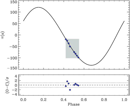
ETV curve of V1200 Cen. Blue diamonds denote the time residuals, derived as explained in Section 3.3.1, while the black line corresponds to the best-fitting solution of the ETV model described by equation (8), considering only the LTTE. The corrections were applied to the measurements, for clarity purpose. The grey area indicates the phase range covered by TESS observations. Fitting residuals are shown in the lower panel.

Open in new tab Download slide

3.3.3 Combined dynamical and LTTE ETV solution

The ETV semi-amplitude of the second effect, very often called ‘physical’ or ‘dynamical’ in the literature, for circular EB orbits is given by (Borkovits et al. 2016)

$$\begin{eqnarray*} A_{\rm phys} = \frac{3}{4\pi } \frac{M_\mathrm{ B}}{M_\mathrm{ A}+M_\mathrm{ B}} \frac{P_1^2}{P_2} \left (1-e_2^2\right)^{-3/2}, \end{eqnarray*}$$

(9)

where the subscripts ‘1’ and ‘2’ refer to the inner and outer orbits, respectively. We have the lower mass limit of M_B (0.871 M_⊙). Thus, we can estimate that A_phys is not smaller than 197 s, making it also a non-negligible effect. Furthermore, if we consider that the B sub-system is composed of two stars with masses lower than |$M_{\mathrm{ Ab}} = 0.8633\,$|M_⊙ (see Section 3.4), then we can put an upper limit to its total mass of 1.727 M_⊙, corresponding to a maximum amplitude of 309 s.

The exact formula for the physical delay in time includes the mutual inclination angle between outer and inner orbits (Rappaport et al. 2013; Borkovits et al. 2015, 2016), which is unknown in our case. Also, on the contrary to the LTTE, this effect cannot be directly derived from the RVs. However, the time coverage of the TESS observations is long enough to see the ETVs manifest in the light curve, as shown in the right-hand panel of Fig. 8. The ETV contribution of the dynamical perturbations takes the following form (Borkovits et al. 2016):

$$\begin{eqnarray*} \Delta _{\rm phys} = A_{\rm phys} \bigg [ \bigg (\frac{2}{3}-\sin ^2 i_{\rm m} \bigg) {\cal M} + \frac{1}{2} \sin ^2 i_{\rm m} {\cal S} \bigg ], \end{eqnarray*}$$

(10)

where

$$\begin{eqnarray*} {\cal M} = 3 e_2 \sin \nu _2 - \frac{3}{4} e_2^2 \sin 2\nu _2 + \frac{1}{3} e_2^3 \sin 3\nu _2 + {\cal O}\left(e_2^4\right), \end{eqnarray*}$$

(11)

and

$$\begin{eqnarray*} {\cal S} = \sin (2\nu _2+2g_2) +e_2 \bigg [ \sin (\nu _2+2g_2) + \frac{1}{3} \sin (3\nu _2+2g_2) \bigg ]. \end{eqnarray*}$$

(12)

Equations (10) to (12) are defined for a circular inner orbit. This approximation appears reasonable here since the eccentricity is small (e₁ = 0.01). In addition, we only need to have a rough estimate of the correction factor to apply to the inner period and thus to the masses of the eclipsing components. By adopting the value of |$M_\mathrm{ B} = 1.727\,$|M_⊙, we can determine the inclination of the outer orbit from the mass function, which we found to be i_AB = 36.3^○. The mutual inclination, i_m, between the two orbital planes is given by (Batten 1973; Fekel 1981):

$$\begin{eqnarray*} \cos i_{\rm m} = \cos i_1 \cos i_2+ \sin i_1 \sin i_2 \cos (\Omega _1-\Omega _2), \end{eqnarray*}$$

(13)

where Ω₁ and Ω₂ are the position angles of the line of nodes of the inner and outer orbits, respectively. In the case of V1200 Cen, these two angles are unknown and thus the mutual inclination i_m cannot be determined. However, it is easy to show from equation (13) that i_A − i_AB ≤ i_m ≤ i_A + i_AB. From the derived values of i_A and i_AB, we then obtain a mutual inclination of 45.1^○ ≤ i_m ≤ 117.7^○. The mutual inclination was set in equation (10) to these limit values during the fit. The only unknown parameter is the dynamical argument of periastron (g₂), which was arbitrarily fixed at zero. We checked that varying this parameter does not change the order of magnitude of the corrections.

Figure 8.

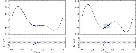
Same as Fig. 7, but taking into account both the LTTE and dynamical perturbation effects for two different values of the mutual inclination, namely i_m = 45.1^○ (left) and i_m = 117.7^○ (right). More details are given in the text.

Open in new tab Download slide

In order to take the dynamical effect into account, the dynamical perturbation term defined in equation (10) was added to equation (8). For each of the two values of i_m, we searched for the values of c₀ and c₁ that best fit the O − C eclipse times, as detailed in Section 3.3.2. The corresponding ETV curves are shown in Fig. 8. When both effects are simultaneously considered, we obtain |$c_0 = 119.8\pm 1.4\,$|s and |$c_1 = -13.1\pm 0.3\,$|s for i_m = 45.1^○, and |$c_0 = 161.4\pm 1.7\,$|s and |$c_1 = -20.3\pm 0.3\,$|s for i_m = 117.7^○. The rms are 1.7 and 2.2 s, respectively. It results that, in the less favourable case, the period value adopted in Table 1 for the eclipsing pair has to be shifted by |$-20.3\,$|s to account for ETVs. Such corrections represent a very small fraction of the period of the eclipsing pair. Thus, the systematic error on the masses M_Aa and M_Ab due to an incorrect estimation of the period should be of |$\Delta P/P = 0.009{{\ \rm per\ cent}}$|⁠, which is largely below the precision claimed in this work (⁠|${\sim }1{{\ \rm per\ cent}}$|⁠).

3.4 Third body in the spectra

The high value of M_B, higher that M_Ab, suggests that the outer body should be easily detectable in the spectra. However, during the RV calculations we have not noticed any prominent third peak in the cross-correlation functions, nor in the TODCOR maps. In order to verify this, we used the formalism of Broadening Function (BF; Rucinski 1992, 2002), and applied it to five CHIRON spectra that have the highest S/N. As a template, we used a spectrum of T_eff = 5200 K, v_rot = 20 km s⁻¹ generated with ATLAS9. A single BF was generated for each of the Echelle orders, and all the single-order BFs were then added in velocity domain, forming the final BF for a given observation. Additionally, we have calculated the expected RVs of the third star, if it had a mass of 0.871 M_⊙ (lower limit of mass, corresponding to the lowest flux contribution). Finally, to check if our approach would recover a small third-light flux, we took one of the spectra (from 2019 August 22) and injected artificial signals at the level of 1 and 3 per cent of the combined brightness of the inner binary. Results are shown in Fig. 9.

Figure 9.

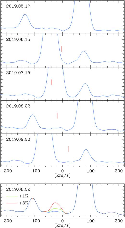
BF analysis of CHIRON spectra. Upper panels show the BFs of five observations with the highest S/N, zoomed so that the secondary peak and background are well visible (primary is out of scale). Red markers indicate velocities of a putative single star of mass equal to the minimum mass of the third body in the system, as found in the orbital solution. No prominent maxima are found on these positions. The lowest panel shows the BFs for one of the spectra, with artificially added third (single star) body that contributes about 1 per cent (green) and 3 per cent (red) to the total flux. Such contribution would have been detected.

Open in new tab Download slide

Two strong peaks, coming from the primary and secondary components, are clearly visible at positions corresponding to their RVs measured with TODCOR. However, no prominent third peak can be seen at positions expected for a 0.871 M_⊙ single star. One can also see that the 3 per cent additional signal is easily detectable, and the 1 per cent signal produces a distinctive peak as well. We therefore conclude that in our CHIRON spectra we would be able to detect the third light of at least 1 per cent level, and that a single star as massive as the secondary is not visible.

Furthermore, at no other RV value we see any indication of a star as bright as the secondary, suggesting that the outer body, even if it is a binary, probably is not composed of such a star. Therefore, we can securely put a conservative upper limit to the total mass of the component B to be 2 × M_Ab = 1.727 M_⊙.

4 DISCUSSION

4.1 Physical parameters of V1200 Cen

From our LC and RV analysis of V1200 Cen, we determined the stellar masses and radii of the eclipsing pair with a better precision than in Coronado et al. (2015). In Table 4, we presented the stellar parameters of each star Aa and Ab, along with their uncertainties, such as derived in this work.

Table 4.

Open in new tab

Stellar parameters and distance of V1200 Cen.

Parameter	Median	84 per cent interval	16 per cent interval
a_Aab (R_⊙)	10.121	+0.037	−0.038
M_Aa (M_⊙)	1.393	+0.018	−0.018
M_Ab (M_⊙)	0.8633	+0.0081	−0.0081
R_Aa (R_⊙)	1.407	+0.014	−0.014
R_Ab (R_⊙)	1.154	+0.014	−0.014
log g_Aa	4.2855	+0.0082	−0.0081
log g_Ab	4.2496	+0.0099	−0.0098
Fe/H	−0.18^a
T_{eff, Aa} (K)	6266^a	±94
T_{eff, Ab} (K)	4650^b	±900
L_Aa [(⁠\|$\log \, (L$\|/L_⊙)]	0.438	+0.026	−0.027
L_Ab [\|$\log \, (L$\|/L_⊙)]	−0.25	+0.30	−0.36
d (pc)	95.7	+5.8	−4.3
π (mas)	10.45	+0.50	−0.60

Parameter	Median	84 per cent interval	16 per cent interval
a_Aab (R_⊙)	10.121	+0.037	−0.038
M_Aa (M_⊙)	1.393	+0.018	−0.018
M_Ab (M_⊙)	0.8633	+0.0081	−0.0081
R_Aa (R_⊙)	1.407	+0.014	−0.014
R_Ab (R_⊙)	1.154	+0.014	−0.014
log g_Aa	4.2855	+0.0082	−0.0081
log g_Ab	4.2496	+0.0099	−0.0098
Fe/H	−0.18^a
T_{eff, Aa} (K)	6266^a	±94
T_{eff, Ab} (K)	4650^b	±900
L_Aa [(⁠\|$\log \, (L$\|/L_⊙)]	0.438	+0.026	−0.027
L_Ab [\|$\log \, (L$\|/L_⊙)]	−0.25	+0.30	−0.36
d (pc)	95.7	+5.8	−4.3
π (mas)	10.45	+0.50	−0.60

Notes. ^aFrom Holmberg, Nordström & Andersen (2009).

^bFrom temperature ratio obtained by Coronado et al. (2015) using phoebe.

Table 4.

Open in new tab

Stellar parameters and distance of V1200 Cen.

Parameter	Median	84 per cent interval	16 per cent interval
a_Aab (R_⊙)	10.121	+0.037	−0.038
M_Aa (M_⊙)	1.393	+0.018	−0.018
M_Ab (M_⊙)	0.8633	+0.0081	−0.0081
R_Aa (R_⊙)	1.407	+0.014	−0.014
R_Ab (R_⊙)	1.154	+0.014	−0.014
log g_Aa	4.2855	+0.0082	−0.0081
log g_Ab	4.2496	+0.0099	−0.0098
Fe/H	−0.18^a
T_{eff, Aa} (K)	6266^a	±94
T_{eff, Ab} (K)	4650^b	±900
L_Aa [(⁠\|$\log \, (L$\|/L_⊙)]	0.438	+0.026	−0.027
L_Ab [\|$\log \, (L$\|/L_⊙)]	−0.25	+0.30	−0.36
d (pc)	95.7	+5.8	−4.3
π (mas)	10.45	+0.50	−0.60

Parameter	Median	84 per cent interval	16 per cent interval
a_Aab (R_⊙)	10.121	+0.037	−0.038
M_Aa (M_⊙)	1.393	+0.018	−0.018
M_Ab (M_⊙)	0.8633	+0.0081	−0.0081
R_Aa (R_⊙)	1.407	+0.014	−0.014
R_Ab (R_⊙)	1.154	+0.014	−0.014
log g_Aa	4.2855	+0.0082	−0.0081
log g_Ab	4.2496	+0.0099	−0.0098
Fe/H	−0.18^a
T_{eff, Aa} (K)	6266^a	±94
T_{eff, Ab} (K)	4650^b	±900
L_Aa [(⁠\|$\log \, (L$\|/L_⊙)]	0.438	+0.026	−0.027
L_Ab [\|$\log \, (L$\|/L_⊙)]	−0.25	+0.30	−0.36
d (pc)	95.7	+5.8	−4.3
π (mas)	10.45	+0.50	−0.60

Notes. ^aFrom Holmberg, Nordström & Andersen (2009).

^bFrom temperature ratio obtained by Coronado et al. (2015) using phoebe.

As can be seen in Table 4, we obtained values of stellar parameters that are in good agreement with those from Coronado et al. (2015), except for the radii of star Ab. Indeed, we found that |$R_{\mathrm{ Ab}} = 1.154\,$|R_⊙ instead of 1.10 R_⊙, i.e. a difference of 5|${{\ \rm per\ cent}}$|⁠. We confirm here the inflated radius of Ab, by about 52 per cent compared to its radius at the zero-age main sequence (ZAMS), which cannot be explained by activity alone and suggests that the star is in its PMS phase of evolution. In the following of the paper, this result will be compared with predictions of stellar models. Another difference comes from the precision of our derived stellar parameters. In particular, we reduced the uncertainties on the stellar mass and radius for the two stars to less than 1.3|${{\ \rm per\ cent}}$|⁠. We then adopted the same effective temperatures as Coronado et al. (2015) to compute the intrinsic luminosities and the distance. In our calculations, we used the bolometric correction (BC) tables¹² from Casagrande & VandenBerg (2018a, b). By considering the values of T_eff, log g, and [Fe/H], listed in Table 4, and an interstellar reddening E(B − V) = 0, we obtained BC_Aa = −0.017 and BC_Ab = −0.451. From the apparent visual magnitude of the system, |$V_{\rm syst} = 8.415\, 2(60)\,$|mag, we then derived a photometric parallax of |$10.45^{+0.50}_{-0.60}\,$|mas for V1200 Cen. This value can be directly compared with the trigonometric parallax from the Gaia Data Release 2 (DR2; Gaia Collaboration 2016, 2018a), namely |$\pi = 9.66 \pm 0.14\,$|mas. We note that our parallax estimate does not match the new Gaia DR2 value within their respective error bars. This difference can be explained by two factors. First, binaries and multiple stellar systems did not receive a special treatment during the Gaia DR2 processing, i.e. the sources were all treated as single stars. As a result, the parallax of such a multiple star can be affected by the orbital motion of the system (Pourbaix 2008). Secondly, our parallax estimate may be biased by the effective temperatures taken from Coronado et al. (2015). An accurate T_eff determination will then be performed in Section 4.3.

Using the values of M_Aa and M_Ab, associated with the quantity f(M_B) in Table 2, we also determined the mass of the third body. We found that |$M_\mathrm{ B} = 0.871\pm 0.020\,$|M_⊙, which corresponds to a minimum value obtained by considering i_AB = 90^○. As explained in Section 3.4, we then attempted to search for signatures of the third body in CHIRON spectra with no success. A possible consequence is that the third body is itself a binary system with two low-mass stars of, for example, |$0.45\,$|M_⊙ each. From our analysis, we argue that V1200 Cen is actually a quadruple-star system with an outer period of 180.4 d instead of 351.5 d. Understanding the formation of close binaries in quadruple-star systems represents a major issue in stellar astrophysics (see Hamers 2019, and references therein), which is beyond the scope of this paper.

4.2 Kinematics

In this work, we checked the validity of the Galactic space velocities (U, V, and W)¹³ derived by Coronado et al. (2015) for V1200 Cen. To this end, we adopted the method developed by Johnson & Soderblom (1987) and implemented in the idl procedure gal_uvw.¹⁴ The input parameters of this procedure are the position (α, δ) at a reference epoch, the parallax π, the proper motion (μ_α*, μ_δ), and the systemic velocity γ_AB. We used the values provided by Gaia Collaboration (2018a), except for γ_AB where the value was taken from our best-fitting RV solution in Table 2. We then obtained |$U = -24.11\pm 0.39\,$|km s⁻¹, |$V = -32.87\pm 0.49\,$|km s⁻¹, and |$W = -10.48\pm 0.22\,$|km s⁻¹. No correction for solar motion was applied. These results are in strong disagreement with those from Coronado et al. (2015) that cannot be explained solely by the different values used as input parameters. Therefore, we suspect that their results are incorrect and that V1200 Cen does not actually belong to the Hyades moving group.

From our new values of the Galactic velocities, we located V1200 Cen at the edge of the Pleiades moving group (PMG; also called the Local Association) following the recent work of Kushniruk, Schirmer & Bensby (2017). The age of the PMG was estimated to be between 110 and 125 Myr (Gaia Collaboration 2018b). It appears that the Pleiades age is more consistent with a young multiple-star system than that of the Hyades (⁠|${\sim} 625\,$|Myr; Perryman et al. 1998). However, we caution the reader that the 110–125 Myr range is only a rough estimate of the systemic age. A more detailed analysis using stellar models is therefore required to precisely determine the individual ages of the eclipsing components (see Section 4.4).

4.3 Effective temperature

The goal of the present section is to constrain the effective temperature of the two eclipsing components with better precision than that reported in previous studies. This parameter is fundamental in order to disentangle between different models for each star, and hence between different ages.

Here, we decided to use the procedure applied by Ribas et al. (1998) to a sample of detached double-lined EBs belonging to the Hipparcos catalogue. This procedure is based on the following expression:

$$\begin{eqnarray*} T_{\rm eff}=\, T_{{\rm eff,}\odot } \left(10\, \pi \frac{R}{\mathrm{ R}_\odot }\right)^{-1/2}\!10^{-0.1(V+{\rm BC}-M_{{\rm bol,}\odot })}, \end{eqnarray*}$$

(14)

where the parallax π is in arcsec and solar values are |$T_{{\rm eff,}\odot }=5777\,$|K and |$M_{{\rm bol,}\odot }=4.74\,$|mag. For each component, the stellar radius is taken from Table 4 and the apparent visual magnitude is computed from the values of V_syst and l₂/l₁ (the secondary-to-primary flux ratio). The corresponding value is |$l_2/l_1=0.0843(44)$|⁠, which was derived using jktebop. We then obtained |$V_{\mathrm{ Aa}}=8.5031(75)\,$|mag and |$V_{Ab}=11.190(53)\,$|mag, with no correction for interstellar extinction. The effective temperature of the two stars was computed by adopting the Gaia DR2 parallax in equation (14). As explained in Section 4.1, the orbital motion of the system can affect the parallax measurement, although we expect this effect to be small. Finally, we adopted the BCs from Casagrande & VandenBerg (2018a, b), which depend on the effective temperature. We then proceeded in an iterative manner to compute the effective temperature of each star using equation (14). We started with a rough estimate of T_eff predicted by stellar models. This allowed us to determine a preliminary value of BC from the Casagrande & VandenBerg (2018a, b) tables. The new T_eff value derived using equation (14), associated with the estimated BC, is then compared to the previous one. We repeated this procedure by adopting the new T_eff value to re-estimate the BC used in equation (14), until convergence. The final results are provided in Table 5, and the corresponding BCs are found to be 0.001 and −0.576 for stars Aa and Ab, respectively.

Table 5.

Open in new tab

Effective temperatures and luminosities of V1200 Cen computed using the Gaia DR2 parallax.

Parameter	Value	1σ error
T_{eff, Aa} (K)	6588	58
T_{eff, Ab} (K)	4475	68
L_Aa [\|$\log \, (L$\|/L_⊙)]	0.525	0.013
L_Ab [\|$\log \, (L$\|/L_⊙)]	−0.319	0.025

Table 5.

Open in new tab

Effective temperatures and luminosities of V1200 Cen computed using the Gaia DR2 parallax.

Parameter	Value	1σ error
T_{eff, Aa} (K)	6588	58
T_{eff, Ab} (K)	4475	68
L_Aa [\|$\log \, (L$\|/L_⊙)]	0.525	0.013
L_Ab [\|$\log \, (L$\|/L_⊙)]	−0.319	0.025

4.4 Comparison with stellar models

This section is dedicated to the comparison between the results from our LC and RV analysis of V1200 Cen and the theoretical predictions from stellar models. The age determination of each of the two eclipsing stars will then help us to shed light on the evolutionary status of V1200 Cen.

4.4.1 mesa isochrones

In order to determine the age of the two stars Aa and Ab, we generated a set of isochrones using a dedicated web interface¹⁵ based on the Modules for Experiments in Stellar Astrophysics (mesa; Paxton et al. 2011, 2013, 2015, 2018) and developed as part of the mesa Isochrones and Stellar Tracks project (MIST v1.2; Choi et al. 2016; Dotter 2016). We considered in this work only the case of non-rotating stars (v/v_crit = 0). For both stars, we first adopted the solar mixture from Asplund et al. (2009), which corresponds to |$Y_{\odot {\rm ,ini}}=0.270\, 3$| and |$Z_{\odot {\rm ,ini}}=0.014\, 2$|⁠. We then searched for the isochrone that best matches the observed parameters (R, M, and T_eff) of each star. We adopted the effective temperatures derived in Section 4.3 and provided in Table 5. Following the previous study of Coronado et al. (2015), we selected isochrones with ages lower than 30 Myr.

The comparison between the observed parameters from our analysis of V1200 Cen and the predictions from mesa isochrones is shown in Fig. 10. For star Aa, we found that the parameters R, M, and T_eff match well the 18.5-Myr isochrone within their 1σ error bars, assuming a solar metallicity. For star Ab, we did not find an isochrone that simultaneously matches these parameters when assuming a solar metallicity. In particular, the predicted T_eff value is underestimated by about 400 K for the best-matching isochrone. The effect of changing the metallicity was then investigated. Finally, we found an isochrone that matches the different parameters for an age of 7 Myr and a metallicity of [Fe/H]_ini = −0.45 (i.e. |$Y_{\rm ini}=0.256\, 8$| and |$Z_{\rm ini}=0.005\, 2$|⁠), as shown in Fig. 10. Furthermore, the precision on the derived parameters allowed us to distinguish between isochrones with an age difference of 1 Myr. These results will be compared with those from another evolutionary code described in the next section.

$Comparison between the observed parameters of V1200 Cen and the predictions from mesa isochrones. Left: Radius versus mass plane (upper panel) and $\log \, T_{\rm eff}$ versus mass plane (lower panel) for star Aa. Green, blue, and red lines correspond to isochrones for ages of 17.5, 18.5, and 19.5 Myr, respectively. Black dots with error bars indicate the derived values of R, M, and $\log \, T_{\rm eff}$ with their corresponding 1σ uncertainties. The Teff value is taken from Table 5. Right: Same as left, but for star Ab and isochrones with the ages indicated in the figure.$

Figure 10.

Comparison between the observed parameters of V1200 Cen and the predictions from mesa isochrones. Left: Radius versus mass plane (upper panel) and |$\log \, T_{\rm eff}$| versus mass plane (lower panel) for star Aa. Green, blue, and red lines correspond to isochrones for ages of 17.5, 18.5, and 19.5 Myr, respectively. Black dots with error bars indicate the derived values of R, M, and |$\log \, T_{\rm eff}$| with their corresponding 1σ uncertainties. The T_eff value is taken from Table 5. Right: Same as left, but for star Ab and isochrones with the ages indicated in the figure.

Open in new tab Download slide

4.4.2 cestam stellar models

We have also fitted the two stars using the cestam stellar evolution code (Morel 1997; Morel & Lebreton 2008; Marques et al. 2013). Models were computed using the OPAL2005 equation of state (Rogers & Nayfonov 2002) and the NACRE nuclear reaction rates (Angulo et al. 1999). We have used the LUNA collaboration reaction rates for ¹⁴N-burning (Imbriani et al. 2005). Convection is treated using the mixing-length theory (Böhm-Vitense 1958) with a mixing length given by αH_P. The value of α that calibrates a solar model computed without diffusion is α = 1.64. We have used the solar mixture of Asplund et al. (2009) in this work. We adopted the OPAL opacity tables (Iglesias & Rogers 1996) calculated with this solar mixture, complemented, at T < 10⁴ K, by the Wichita opacity data (Ferguson et al. 2005). The atmosphere was treated using the Eddington grey approximation.

We have found it impossible to fit both stars with the same age and chemical composition. The Aa component is easily fitted with a solar metallicity (Z = 0.0134; Asplund et al. 2009); its effective temperature and luminosity are reached at an age of 16 Myr. However, the model for the Ab component at the same age has an effective temperature and a luminosity that are lower than those observed. This is shown in the left-hand panel of Fig. 11.

Figure 11.

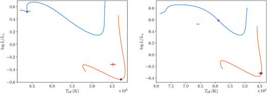
Evolutionary tracks in the HR diagram of models calculated with a solar metallicity (left-hand panel) and Z = 0.005 (right-hand panel). Circles on the tracks indicate models with an age of 16 Myr (left-hand panel) and 5.5 Myr (right-hand panel).

Open in new tab Download slide

The Ab component can be fitted with a metallicity Z = 0.005. We obtain an effective temperature and a luminosity that are consistent with the observations at an age of 5.5 ± 1 Myr. However, the model for the Aa component is now too cold and bright at the same age, as seen in the right-hand panel of Fig. 11.

These results are consistent with the previous section.

4.4.3 Evolutionary status of V1200 Cen

Using two different stellar models, we determined the individual age of each eclipsing component of the system from their observed parameters. We obtained a good agreement between mesa and cestam models. In particular, individual ages are found to be 16–18.5 and 5.5–7 Myr for stars Aa and Ab, respectively. Furthermore, both models fail to reproduce the observed parameters of star Ab when assuming a solar metallicity. A lower metallicity is then required to properly fit the Ab component, while a solar metallicity is adopted for the Aa component.

Due to their common origin, stars belonging to a binary or multiple system are usually assumed to have the same age and initial chemical composition. However, the eclipsing components of V1200 Cen appear to be non-coeval with a difference in age as high as ∼65 per cent. In addition to the age difference, the metallicity needed to fit the Ab component is lower by a factor of ∼2.7 than that of the Aa component, independently of the model used. If we consider that the secondary star has the same age and chemical composition as the primary star, then the observed parameters of the secondary are in clear disagreement with the predictions from both mesa and cestam. The secondary star is indeed hotter, larger, and thus brighter than that predicted by the evolutionary track for that age. In the opposite case, i.e. when the age of the secondary star is considered, the effective temperature of the primary is too high by about 700 K, making this hypothesis unlikely. Such discrepancies have already been reported by Lacy et al. (2016) for another PMS EB, namely NP Persei. In particular, the authors found that the two components of NP Per cannot be fitted at a single age, implying a relative age difference of about 44 per cent. Stellar activity was proposed as a possible explanation for the discrepancies between the observed and predicted properties of NP Per. However, based on the analysis of 13 PMS EBs, Stassun et al. (2014) concluded that activity alone cannot fully explain the discrepancies observed for this kind of systems. Stassun et al. (2014) also noticed that half of their binaries have a tertiary companion. In the case of NP Per, its short orbital period of 2.2 d could suggest the presence of an undetected companion in a wide orbit.

The influence of a third body on the evolution of the eclipsing pair was investigated in detail by Stassun et al. (2014). Based on their conclusions, the evolutionary status of V1200 Cen can be described as follows. This quadruple-star system was likely formed 16–18.5 Myr ago from a small gas cloud. The inner orbits were originally almost perpendicular to the outer orbit, allowing Lidov–Kozai cycles to take place. Both inner orbits acquired high eccentricity, thereby making the dynamical interaction between the four stars possible. Each sub-system is then circularized and tightened owing to their mutual influence. Once both inner orbits have been circularized, the two components of each system continue to interact by tidal effects, as their radii are still large compared to their separation. Such dynamical and tidal interactions may alter the stellar properties, resulting in the apparent non-coevality of the eclipsing components of V1200 Cen.

4.5 Confirmation of the quadruple nature of V1200 Cen

4.5.1 Limitations of the single-star scenario for V1200 Cen B

If we consider that the third star has the same age as the primary, then the flux ratio between the tertiary and the secondary is about 0.6 in the TESS band. In this case, the contribution of the third star to the total light is 7 per cent (more details will be given in Section 4.5.2). We can also consider that the third star has an inflated radius that is nearly equal to that of the secondary star, implying a similar luminosity at the age of the secondary isochrone. In addition, Tokovinin (2017) showed that the mutual inclination in compact low-mass triples is on average of 20^○. Assuming this value, we obtain two possible configurations for the stellar system, which correspond to an inclination of the third-body orbit of about 61^○ and 101^○, respectively. The corresponding masses are, respectively, |${\sim }1.02$| and |${\sim }0.89\,$|M_⊙. The lower value is very close to that derived from the mass function. Depending on the isochrone, the flux ratio l₃/l₂ is expected to lie in the range 0.7–1.2. However, for the higher value of M_B, the flux ratio is found to be between 1.6 and 2.6. It appears that for a mass higher than |${\sim }0.95\,$|M_⊙, the lines of the third star should be present in the spectrum. This limit corresponds to a reasonable mutual inclination of about 13^○ (i_AB ≃ 68^○). Below this limit, the third light still represents more than 7 per cent of the total flux that is inconsistent with the results of the LC and BF analyses, where the third star contribution is not detected. Therefore, we think that it is more likely that the third body is a binary system with two low-mass stars, each contributing to 1.5 per cent or less of the total flux when assuming stellar masses of 0.45 M_⊙ (see Section 4.5.2 below).

4.5.2 Third-light contribution of the B sub-system

We investigated the impact on the derived stellar parameters of varying the third light during the light-curve analysis. For this, we adopted l₃/l_tot = [0.03, 0.07, 0.12, 0.18], where the two first values are taken from the model predictions obtained in Section 4.5.1. The corresponding stellar parameters are listed in Table 6.

Table 6.

Open in new tab

Stellar parameters of V1200 Cen as a function of the third-light contribution. The first line corresponds to our reference model (see Table 4).

l₃/l_tot	i_A	R_Aa	R_Ab	M_Aa	M_Ab
(per cent)	(^○)	(R_⊙)	(R_⊙)	(M_⊙)	(M_⊙)
0	81.38	1.407	1.154	1.393	0.8633
3	81.49	1.387	1.158	1.392	0.8625
7	81.66	1.350	1.175	1.390	0.8614
12	81.77	1.314	1.198	1.389	0.8607
18	81.92	1.250	1.245	1.387	0.8597

l₃/l_tot	i_A	R_Aa	R_Ab	M_Aa	M_Ab
(per cent)	(^○)	(R_⊙)	(R_⊙)	(M_⊙)	(M_⊙)
0	81.38	1.407	1.154	1.393	0.8633
3	81.49	1.387	1.158	1.392	0.8625
7	81.66	1.350	1.175	1.390	0.8614
12	81.77	1.314	1.198	1.389	0.8607
18	81.92	1.250	1.245	1.387	0.8597

Table 6.

Open in new tab

Stellar parameters of V1200 Cen as a function of the third-light contribution. The first line corresponds to our reference model (see Table 4).

l₃/l_tot	i_A	R_Aa	R_Ab	M_Aa	M_Ab
(per cent)	(^○)	(R_⊙)	(R_⊙)	(M_⊙)	(M_⊙)
0	81.38	1.407	1.154	1.393	0.8633
3	81.49	1.387	1.158	1.392	0.8625
7	81.66	1.350	1.175	1.390	0.8614
12	81.77	1.314	1.198	1.389	0.8607
18	81.92	1.250	1.245	1.387	0.8597

l₃/l_tot	i_A	R_Aa	R_Ab	M_Aa	M_Ab
(per cent)	(^○)	(R_⊙)	(R_⊙)	(M_⊙)	(M_⊙)
0	81.38	1.407	1.154	1.393	0.8633
3	81.49	1.387	1.158	1.392	0.8625
7	81.66	1.350	1.175	1.390	0.8614
12	81.77	1.314	1.198	1.389	0.8607
18	81.92	1.250	1.245	1.387	0.8597

It is notable that the secondary radius increases with increasing third light, whereas the primary radius decreases. The last case in Table 6 corresponds to a third star having almost the same flux contribution as the secondary (⁠|$l_2/l_{\rm tot} = 21{{\ \rm per\ cent}}$|⁠). In this case, the primary and secondary stars have similar radii of 1.250 and 1.245 R_⊙, respectively, while their masses remain nearly unchanged compared to our reference model. The consequence is that the primary star appears to be older and the secondary younger than that previously estimated, implying an even higher age difference. In addition, when we consider the case of a second binary that contributes to 3 per cent of the total flux, the primary and secondary radii differ by −1.5σ and +0.3σ from the reference values, respectively. These values are in better agreement than those obtained considering a single star, which contributes 7 per cent to the total flux. In this latter case, the stellar radii differ by −4.2σ and +1.5σ for the primary and the secondary, respectively. For all cases, the goodness of fit is similar due to the correlations linking the third-light parameter to the other parameters (i, r₁, and r₂).

5 SUMMARY

The aim of this work was to perform a new analysis of V1200 Centauri, a multiple-star system that contains a close EB. For this, we made use of the most recent observations of the system from the Solaris network, the TESS space telescope, and the CHIRON spectrograph. The combined analysis of the light curves and RV measurements allowed us to derive the mass and radius of each eclipsing component with a precision better than 1.3 per cent. The resulting values for the primary component are |$M_{\mathrm{ Aa}} = 1.393\pm 0.018\,$|M_⊙ and |$R_{\mathrm{ Aa}} = 1.407\pm 0.014\,$|R_⊙. For the secondary, we found that |$M_{\mathrm{ Ab}} = 0.8633\pm 0.0081\,$|M_⊙ and |$R_{\mathrm{ Ab}} = 1.154\pm 0.014\,$|R_⊙, where the inflated radius confirms the PMS nature of the system. We also confirmed the 2.5-d orbital period of the eclipsing pair, whereas the eccentricity was found to be slightly different from zero (e = 0.01). However, regarding the outer orbit, we obtained significantly different results than those reported in the literature. Thanks to the additional measurements from CHIRON, we derived a new orbital solution assuming an outer period of 180.4 d, instead of 351.5 d, and a minimum mass for the third body of |$0.871\pm 0.020\,$|M_⊙. A consequence of this result is that the third body is actually a binary system with two low-mass stars that are not detectable from our observations. V1200 Centauri is thus a quadruple-star system consisting of two close pairs orbiting each other with a 180-d period.

Finally, we compared the observed parameters of each eclipsing components with the predictions from two independent stellar evolution codes, namely mesa and cestam. In addition to the mass and radius, we also used the effective temperatures derived in this work to better constrain the individual ages of the eclipsing components. From their radii and apparent magnitudes, we found the effective temperatures of the stars to be |$T_{{\rm eff},\mathrm{ Aa}} = 6588\pm 58\,$|K and |$T_{{\rm eff},\mathrm{ Ab}} = 4475\pm 68\,$|K when adopting the Gaia DR2 parallax. We then obtained ages of 16–18.5 and 5.5–7 Myr for stars Aa and Ab, respectively. Despite the good agreement between mesa and cestam models, we failed to reproduce the observed parameters by assuming the same age and chemical composition for both stars. In particular, it is noticeable that the secondary star appears both larger and hotter than that predicted at the age of the primary. For V1200 Cen, the relative age difference is particularly high (∼65 per cent). However, it is likely that the stars in such a close quadruple system experienced strong dynamical and tidal interactions, possibly affecting the observed stellar parameters. In conclusion, the case of V1200 Centauri provides a real challenge for theoreticians to model PMS stars in multiple systems, and to account for their apparent non-coevality.

ACKNOWLEDGEMENTS

Based on data collected with Solaris network of telescopes of the Nicolaus Copernicus Astronomical Center of the Polish Academy of Sciences. This paper includes data collected by the TESS mission, which are publicly available from the MAST. Funding for the TESS mission is provided by NASA’s Science Mission directorate. This research made use of Photutils, an Astropy package for detection and photometry of astronomical sources (Bradley et al. 2019). This work has made use of data from the European Space Agency (ESA) mission Gaia (https://www.cosmos.esa.int/gaia), processed by the Gaia Data Processing and Analysis Consortium (DPAC; https://www.cosmos.esa.int/web/gaia/dpac/consortium). Funding for the DPAC has been provided by national institutions, in particular the institutions participating in the Gaia Multilateral Agreement. This research has made use of NASA’s Astrophysics Data System Bibliographic Services, the SIMBAD data base, operated at CDS, Strasbourg, France and the VizieR catalogue access tool, CDS, Strasbourg, France. The original description of the VizieR service was published in Ochsenbein, Bauer & Marcout (2000).

We acknowledge support provided by the Polish National Science Center (NCN) through grants 2017/27/B/ST9/02727 (FM and MK), 2016/21/B/ST9/01613 (KGH), and 2015/16/S/ST9/00461 (MR).

Finally, we also thank the anonymous referee for comments that helped us to improve this paper.

DATA AVAILABILITY

The data underlying this article will be shared on reasonable request to the corresponding author.

Footnotes

1

https://www.saao.ac.za/

2

https://www.sidingspringobservatory.com.au/

3

https://casleo.conicet.gov.ar/

4

https://photutils.readthedocs.io/en/stable/

5

https://github.com/hippke/wotan

6

Guest Investigator programme G011083, PI: Hełminiak.

7

https://archive.stsci.edu/

8

More details are given in the DR note of sector 11 (DR16) available at https://archive.stsci.edu/tess/tess_drn.html.

9

https://www.astro.keele.ac.uk/~jkt/codes.html

10

For more details, see Vanzi et al. (2012).

11

For more details, see Queloz et al. (2001).

12

https://github.com/casaluca/bolometric-corrections

13

The values of U, V, and W are positive in the directions of the Galactic Centre, rotation, and north pole, respectively.

14

https://idlastro.gsfc.nasa.gov/ftp/pro/astro/gal_uvw.pro

15

http://waps.cfa.harvard.edu/MIST/

REFERENCES

Angulo

C.

et al. ,

1999

,

Nucl. Phys. A

,

656

,

3

10.1016/S0375-9474(99)00030-5

Crossref

Search ADS

Asplund

M.

,

Grevesse

N.

,

Sauval

A. J.

,

Scott

P.

,

2009

,

ARA&A

,

47

,

481

10.1146/annurev.astro.46.060407.145222

Crossref

Search ADS

Batten

A. H.

,

1973

,

Binary and Multiple Systems of Stars

,

Pergamon Press

,

Oxford

Böhm-Vitense

E.

,

1958

,

Z. Astrophys.

,

46

,

108

Borkovits

T.

,

Rappaport

S.

,

Hajdu

T.

,

Sztakovics

J.

,

2015

,

MNRAS

,

448

,

946

10.1093/mnras/stv015

Crossref

Search ADS

Borkovits

T.

,

Hajdu

T.

,

Sztakovics

J.

,

Rappaport

S.

,

Levine

A.

,

Bíró

I. B.

,

Klagyivik

P.

,

2016

,

MNRAS

,

455

,

4136

10.1093/mnras/stv2530

Crossref

Search ADS

Bradley

L.

et al. ,

2019

,

Astropy/Photutils: v0.6

, available at: https://zenodo.org/record/2533376

Casagrande

L.

,

VandenBerg

D. A.

,

2018a

,

MNRAS

,

475

,

5023

10.1093/mnras/sty149

Crossref

Search ADS

Casagrande

L.

,

VandenBerg

D. A.

,

2018b

,

MNRAS

,

479

,

L102

10.1093/mnrasl/sly104

Crossref

Search ADS

Choi

J.

,

Dotter

A.

,

Conroy

C.

,

Cantiello

M.

,

Paxton

B.

,

Johnson

B. D.

,

2016

,

ApJ

,

823

,

102

10.3847/0004-637X/823/2/102

Crossref

Search ADS

Coronado

J.

et al. ,

2015

,

MNRAS

,

448

,

1937

10.1093/mnras/stv010

Crossref

Search ADS

Dotter

A.

,

2016

,

ApJS

,

222

,

8

10.3847/0067-0049/222/1/8

Crossref

Search ADS

Fekel

F. C.

Jr,

1981

,

ApJ

,

246

,

879

10.1086/158981

Crossref

Search ADS

Ferguson

J. W.

,

Alexander

D. R.

,

Allard

F.

,

Barman

T.

,

Bodnarik

J. G.

,

Hauschildt

P. H.

,

Heffner-Wong

A.

,

Tamanai

A.

,

2005

,

ApJ

,

623

,

585

Crossref

Search ADS

Gaia Collaboration

,

2016

,

A&A

,

595

,

A1

10.1051/0004-6361/201629272

Crossref

Search ADS

Gaia Collaboration

,

2018a

,

A&A

,

616

,

A1

10.1051/0004-6361/201833051

Crossref

Search ADS

Gaia Collaboration

,

2018b

,

A&A

,

616

,

A10

10.1051/0004-6361/201832843

Crossref

Search ADS

Gómez Maqueo Chew

Y.

et al. ,

2019

,

A&A

,

623

,

A23

10.1051/0004-6361/201833299

Crossref

Search ADS

Hamers

A. S.

,

2019

,

MNRAS

,

482

,

2262

10.1093/mnras/sty2879

Crossref

Search ADS

Hastings

W. K.

,

1970

,

Biometrika

,

57

,

97

10.1093/biomet/57.1.97

Crossref

Search ADS

Hełminiak

K. G.

et al. ,

2012

,

MNRAS

,

425

,

1245

10.1111/j.1365-2966.2012.21510.x

Crossref

Search ADS

Hełminiak

K. G.

,

Ukita

N.

,

Kambe

E.

,

Kozłowski

S. K.

,

Sybilski

P.

,

Ratajczak

M.

,

Maehara

H.

,

Konacki

M.

,

2016

,

MNRAS

,

461

,

2896

10.1093/mnras/stw1514

Crossref

Search ADS

Hilditch

R. W.

,

2001

,

An Introduction to Close Binary Stars

,

Cambridge Univ. Press

,

Cambridge

Hippke

M.

,

David

T. J.

,

Mulders

G. D.

,

Heller

R.

,

2019

,

AJ

,

158

,

143

10.3847/1538-3881/ab3984

Crossref

Search ADS

Holmberg

J.

,

Nordström

B.

,

Andersen

J.

,

2009

,

A&A

,

501

,

941

10.1051/0004-6361/200811191

Crossref

Search ADS

Iglesias

C. A.

,

Rogers

F. J.

,

1996

,

ApJ

,

464

,

943

10.1086/177381

Crossref

Search ADS

Imbriani

G.

et al. ,

2005

,

Eur. Phys. J. A

,

25

,

455

Crossref

Search ADS

Irwin

J. B.

,

1952

,

ApJ

,

116

,

211

10.1086/145604

Crossref

Search ADS

Jenkins

J. M.

et al. ,

2016

, in

Gianluca

C.

,

Juan

C. G.

, eds,

Proc. SPIE Conf. Ser. Vol. 9913, Software and Cyberinfrastructure for Astronomy IV

.

SPIE

,

Bellingham

, p.

99133E

10.1117/12.2233418

Google Scholar

Google Preview

OpenURL Placeholder Text

WorldCat

Crossref

Johnson

D. R. H.

,

Soderblom

D. R.

,

1987

,

AJ

,

93

,

864

10.1086/114370

Crossref

Search ADS

Klinglesmith

D. A.

,

Sobieski

S.

,

1970

,

AJ

,

75

,

175

10.1086/110960

Crossref

Search ADS

Konacki

M.

,

Sybilski

P.

,

Kozłowski

S. K.

,

Ratajczak

M.

,

Hełminiak

K. G.

,

2012

, in

Richards

M. T.

,

Hubeny

I.

, eds,

Proc. IAU Symp. 282, From Interacting Binaries to Exoplanets: Essential Modeling Tools

.

Kluwer

,

Dordrecht

, p.

111

10.1017/S1743921311027098

Google Scholar

Google Preview

OpenURL Placeholder Text

WorldCat

Crossref

Kopal

Z.

,

1959

,

Close Binary Systems

.

Kozai

Y.

,

1962

,

AJ

,

67

,

591

10.1086/108790

Crossref

Search ADS

Kozłowski

S. K.

,

Sybilski

P.

,

Konacki

M.

,

Pawłaszek

R. K.

,

Ratajczak

M.

,

Helminiak

K. G.

,

2014

, in

Larry

M. S.

,

Roberto

G.

, eds,

Proc. SPIE Conf. Ser. Vol. 9145, Ground-Based and Airborne Telescopes V

.

SPIE

,

Bellingham

, p.

914504

10.1117/12.2055620

Google Scholar

Google Preview

OpenURL Placeholder Text

WorldCat

Crossref

Kozłowski

S. K.

,

Sybilski

P. W.

,

Konacki

M.

,

Pawłaszek

R. K.

,

Ratajczak

M.

,

Hełminiak

K. G.

,

Litwicki

M.

,

2017

,

PASP

,

129

,

105001

10.1088/1538-3873/aa83aa

Crossref

Search ADS

Kushniruk

I.

,

Schirmer

T.

,

Bensby

T.

,

2017

,

A&A

,

608

,

A73

10.1051/0004-6361/201731147

Crossref

Search ADS

Lacy

C. H. S.

,

Fekel

F. C.

,

Pavlovski

K.

,

Torres

G.

,

Muterspaugh

M. W.

,

2016

,

AJ

,

152

,

2

10.3847/0004-6256/152/1/2

Crossref

Search ADS

Lidov

M. L.

,

1962

,

Planet. Space Sci.

,

9

,

719

10.1016/0032-0633(62)90129-0

Crossref

Search ADS

Lomb

N. R.

,

1976

,

Ap&SS

,

39

,

447

10.1007/BF00648343

Crossref

Search ADS

Marcadon

F.

,

Appourchaux

T.

,

Marques

J. P.

,

2018

,

A&A

,

617

,

A2

10.1051/0004-6361/201731628

Crossref

Search ADS

Marques

J. P.

et al. ,

2013

,

A&A

,

549

,

A74

10.1051/0004-6361/201220211

Crossref

Search ADS

Mayer

P.

,

1990

,

Bull. Astron. Inst. Czech.

,

41

,

231

Mazeh

T.

,

Zucker

S.

,

1994

,

Ap&SS

,

212

,

349

10.1007/BF00984538

Crossref

Search ADS

Metropolis

N.

,

Rosenbluth

A. W.

,

Rosenbluth

M. N.

,

Teller

A. H.

,

Teller

E.

,

1953

,

J. Chem. Phys.

,

21

,

1087

10.1063/1.1699114

Crossref

Mikulášek

Z.

,

2015

,

A&A

,

584

,

A8

10.1051/0004-6361/201425244

Crossref

Search ADS

Morel

P.

,

1997

,

A&AS

,

124

,

597

10.1051/aas:1997209

Crossref

Search ADS

Morel

P.

,

Lebreton

Y.

,

2008

,

Ap&SS

,

316

,

61

10.1007/s10509-007-9663-9

Crossref

Search ADS

Munari

U.

et al. ,

2014

,

AJ

,

148

,

81

10.1088/0004-6256/148/5/81

Crossref

Search ADS

Ochsenbein

F.

,

Bauer

P.

,

Marcout

J.

,

2000

,

A&AS

,

143

,

23

10.1051/aas:2000169

Crossref

Search ADS

Paczyński

B.

,

Szczygieł

D. M.

,

Pilecki

B.

,

Pojmański

G.

,

2006

,

MNRAS

,

368

,

1311

10.1111/j.1365-2966.2006.10223.x

Crossref

Search ADS

Paxton

B.

et al. ,

2013

,

ApJS

,

208

,

4

10.1088/0067-0049/208/1/4

Crossref

Search ADS

Paxton

B.

et al. ,

2015

,

ApJS

,

220

,

15

10.1088/0067-0049/220/1/15

Crossref

Search ADS

Paxton

B.

et al. ,

2018

,

ApJS

,

234

,

34

10.3847/1538-4365/aaa5a8

Crossref

Search ADS

Paxton

B.

,

Bildsten

L.

,

Dotter

A.

,

Herwig

F.

,

Lesaffre

P.

,

Timmes

F.

,

2011

,

ApJS

,

192

,

3

10.1088/0067-0049/192/1/3

Crossref

Search ADS

Perryman

M. A. C.

et al. ,

1998

,

A&A

,

331

,

81

Pojmanski

G.

,

2002

,

Acta Astron.

,

52

,

397

Pollacco

D. L.

et al. ,

2006

,

PASP

,

118

,

1407

10.1086/508556

Crossref

Search ADS

Popper

D. M.

,

Etzel

P. B.

,

1981

,

AJ

,

86

,

102

10.1086/112862

Crossref

Search ADS

Pourbaix

D.

,

2008

, in

Jin

W. J.

,

Platais

I.

,

Perryman

M. A. C.

, eds,

Proc. IAU Symp. 248, A Giant Step: from Milli- to Micro-arcsecond Astrometry

.

Kluwer

,

Dordrecht

, p.

59

10.1017/S1743921308018632

Google Scholar

Google Preview

OpenURL Placeholder Text

WorldCat

Crossref

Queloz

D.

et al. ,

2001

,

The Messenger

,

105

,

1

Rappaport

S.

,

Deck

K.

,

Levine

A.

,

Borkovits

T.

,

Carter

J.

,

El Mellah

I.

,

Sanchis-Ojeda

R.

,

Kalomeni

B.

,

2013

,

ApJ

,

768

,

33

10.1088/0004-637X/768/1/33

Crossref

Search ADS

Ribas

I.

,

Gimenez

A.

,

Torra

J.

,

Jordi

C.

,

Oblak

E.

,

1998

,

A&A

,

330

,

600

Ricker

G. R.

et al. ,

2015

,

J. Astron. Telesc. Instrum. Syst.

,

1

,

014003

10.1117/1.JATIS.1.1.014003

Crossref

Search ADS

Rogers

F. J.

,

Nayfonov

A.

,

2002

,

ApJ

,

576

,

1064

10.1086/341894

Crossref

Search ADS

Rucinski

S. M.

,

1992

,

AJ

,

104

,

1968

10.1086/116372

Crossref

Search ADS

Rucinski

S. M.

,

2002

,

AJ

,

124

,

1746

10.1086/342342

Crossref

Search ADS

Scargle

J. D.

,

1982

,

ApJ

,

263

,

835

10.1086/160554

Crossref

Search ADS

Schwab

C.

,

Spronck

J. F. P.

,

Tokovinin

A.

,

Szymkowiak

A.

,

Giguere

M.

,

Fischer

D. A.

,

2012

, in

McLean

I. S.

,

Ramsay

S. K.

,

Takami

H.

, eds,

Proc. SPIE Conf. Ser. Vol. 8446, Ground-based and Airborne Instrumentation for Astronomy IV

,

SPIE

,

Bellingham

, p.

84460B

10.1117/12.925108

Google Scholar

Google Preview

OpenURL Placeholder Text

WorldCat

Crossref

Smith

J. C.

et al. ,

2012

,

PASP

,

124

,

1000

10.1086/667697

Crossref

Search ADS

Southworth

J.

,

Maxted

P. F. L.

,

Smalley

B.

,

2004a

,

MNRAS

,

351

,

1277

10.1111/j.1365-2966.2004.07871.x

Crossref

Search ADS

Southworth

J.

,

Zucker

S.

,

Maxted

P. F. L.

,

Smalley

B.

,

2004b

,

MNRAS

,

355

,

986

10.1111/j.1365-2966.2004.08389.x

Crossref

Search ADS

Southworth

J.

,

Smalley

B.

,

Maxted

P. F. L.

,

Claret

A.

,

Etzel

P. B.

,

2005

,

MNRAS

,

363

,

529

10.1111/j.1365-2966.2005.09462.x

Crossref

Search ADS

Stassun

K. G.

,

Feiden

G. A.

,

Torres

G.

,

2014

,

New Astron. Rev.

,

60

,

1

10.1016/j.newar.2014.06.001

Crossref

Search ADS

Stumpe

M. C.

et al. ,

2012

,

PASP

,

124

,

985

10.1086/667698

Crossref

Search ADS

Stumpe

M. C.

,

Smith

J. C.

,

Catanzarite

J. H.

,

Van Cleve

J. E.

,

Jenkins

J. M.

,

Twicken

J. D.

,

Girouard

F. R.

,

2014

,

PASP

,

126

,

100

10.1086/674989

Crossref

Search ADS

Tohline

J. E.

,

2002

,

ARA&A

,

40

,

349

10.1146/annurev.astro.40.060401.093810

Crossref

Search ADS

Tokovinin

A.

,

2008

,

MNRAS

,

389

,

925

10.1111/j.1365-2966.2008.13613.x

Crossref

Search ADS

Tokovinin

A.

,

2017

,

ApJ

,

844

,

103

10.3847/1538-4357/aa7746

Crossref

Search ADS

Tokovinin

A.

,

Fischer

D. A.

,

Bonati

M.

,

Giguere

M. J.

,

Moore

P.

,

Schwab

C.

,

Spronck

J. F. P.

,

Szymkowiak

A.

,

2013

,

PASP

,

125

,

1336

10.1086/674012

Crossref

Search ADS

Toonen

S.

,

Hamers

A.

,

Portegies Zwart

S.

,

2016

,

Comput. Astrophys. Cosmol.

,

3

,

6

10.1186/s40668-016-0019-0

Crossref

Search ADS

Torres

G.

,

Andersen

J.

,

Giménez

A.

,

2010

,

A&AR

,

18

,

67

10.1007/s00159-009-0025-1

Crossref

Search ADS

Tran

K.

,

Levine

A.

,

Rappaport

S.

,

Borkovits

T.

,

Csizmadia

S.

,

Kalomeni

B.

,

2013

,

ApJ

,

774

,

81

10.1088/0004-637X/774/1/81

Crossref

Search ADS

van Hamme

W.

,

1993

,

AJ

,

106

,

2096

10.1086/116788

Crossref

Search ADS

Vanzi

L.

et al. ,

2012

,

MNRAS

,

424

,

2770

10.1111/j.1365-2966.2012.21382.x

Crossref

Search ADS

APPENDIX A: RADIAL VELOCITIES

In Table A1, we listed all the RV measurements of V1200 Cen used in this study, together with the final measurement errors σ. For the sake of clarity, we kept the notation introduced by Coronado et al. (2015), where indices 1 and 2 refer, respectively, to the primary and secondary components (Aa and Ab) of the eclipsing pair. The last column shows the telescope/spectrograph used, coded as follows: 5/P = OUC 50-cm/PUCHEROS, E/C = Euler 1.2-m/CORALIE, C/C = CTIO 1.5-m/CHIRON.

Table A1.

Open in new tab

Individual RV measurements of V1200 Cen used in this work. All values are given in km s⁻¹.

JD\|$-245\,0000$\|	v₁	σ₁	v₂	σ₂	Tel./Sp.
5714.615 861	45.958	0.646	–	–	5/P
5736.539 995	64.395	0.494	−127.519	2.640	5/P
5737.639 889	−67.029	0.523	88.377	4.198	5/P
5750.604 835	−62.826	2.446	–	–	5/P
5751.584 224	74.651	0.536	−126.370	4.324	5/P
6066.642 808	47.460	1.498	–	–	5/P
6066.665 643	51.655	0.841	–	–	5/P
6078.565 477	−36.335	2.129	–	–	5/P
6080.625 298	−89.867	0.163	112.325	1.503	E/C
6081.564 728	52.113	0.228	−116.745	1.075	E/C
6179.474 281	−26.024	0.167	80.336	0.885	E/C
6346.690 592	−12.831	0.169	67.855	0.876	E/C
6348.857 536	−55.020	0.165	136.192	1.064	E/C
6349.894 755	94.865	0.194	−107.687	1.017	E/C
6397.520 928	38.353	0.112	−71.655	0.772	E/C
6398.517 694	−77.575	0.116	112.000	0.951	E/C
6497.610 599	−67.667	0.157	133.439	0.797	E/C
6498.610 654	64.361	0.113	−78.099	0.942	E/C
8621.784 282	69.037	0.134	−134.418	0.739	C/C
8650.705 804	−42.656	0.146	76.048	0.869	C/C
8680.534 650	−23.882	0.134	81.379	0.520	C/C
8696.577 977	73.578	0.337	−70.828	2.379	C/C
8718.466 921	80.631	0.131	−106.965	1.035	C/C
8747.475 367	−62.708	0.138	82.865	0.655	C/C

JD\|$-245\,0000$\|	v₁	σ₁	v₂	σ₂	Tel./Sp.
5714.615 861	45.958	0.646	–	–	5/P
5736.539 995	64.395	0.494	−127.519	2.640	5/P
5737.639 889	−67.029	0.523	88.377	4.198	5/P
5750.604 835	−62.826	2.446	–	–	5/P
5751.584 224	74.651	0.536	−126.370	4.324	5/P
6066.642 808	47.460	1.498	–	–	5/P
6066.665 643	51.655	0.841	–	–	5/P
6078.565 477	−36.335	2.129	–	–	5/P
6080.625 298	−89.867	0.163	112.325	1.503	E/C
6081.564 728	52.113	0.228	−116.745	1.075	E/C
6179.474 281	−26.024	0.167	80.336	0.885	E/C
6346.690 592	−12.831	0.169	67.855	0.876	E/C
6348.857 536	−55.020	0.165	136.192	1.064	E/C
6349.894 755	94.865	0.194	−107.687	1.017	E/C
6397.520 928	38.353	0.112	−71.655	0.772	E/C
6398.517 694	−77.575	0.116	112.000	0.951	E/C
6497.610 599	−67.667	0.157	133.439	0.797	E/C
6498.610 654	64.361	0.113	−78.099	0.942	E/C
8621.784 282	69.037	0.134	−134.418	0.739	C/C
8650.705 804	−42.656	0.146	76.048	0.869	C/C
8680.534 650	−23.882	0.134	81.379	0.520	C/C
8696.577 977	73.578	0.337	−70.828	2.379	C/C
8718.466 921	80.631	0.131	−106.965	1.035	C/C
8747.475 367	−62.708	0.138	82.865	0.655	C/C

Table A1.

Open in new tab

Individual RV measurements of V1200 Cen used in this work. All values are given in km s⁻¹.

JD\|$-245\,0000$\|	v₁	σ₁	v₂	σ₂	Tel./Sp.
5714.615 861	45.958	0.646	–	–	5/P
5736.539 995	64.395	0.494	−127.519	2.640	5/P
5737.639 889	−67.029	0.523	88.377	4.198	5/P
5750.604 835	−62.826	2.446	–	–	5/P
5751.584 224	74.651	0.536	−126.370	4.324	5/P
6066.642 808	47.460	1.498	–	–	5/P
6066.665 643	51.655	0.841	–	–	5/P
6078.565 477	−36.335	2.129	–	–	5/P
6080.625 298	−89.867	0.163	112.325	1.503	E/C
6081.564 728	52.113	0.228	−116.745	1.075	E/C
6179.474 281	−26.024	0.167	80.336	0.885	E/C
6346.690 592	−12.831	0.169	67.855	0.876	E/C
6348.857 536	−55.020	0.165	136.192	1.064	E/C
6349.894 755	94.865	0.194	−107.687	1.017	E/C
6397.520 928	38.353	0.112	−71.655	0.772	E/C
6398.517 694	−77.575	0.116	112.000	0.951	E/C
6497.610 599	−67.667	0.157	133.439	0.797	E/C
6498.610 654	64.361	0.113	−78.099	0.942	E/C
8621.784 282	69.037	0.134	−134.418	0.739	C/C
8650.705 804	−42.656	0.146	76.048	0.869	C/C
8680.534 650	−23.882	0.134	81.379	0.520	C/C
8696.577 977	73.578	0.337	−70.828	2.379	C/C
8718.466 921	80.631	0.131	−106.965	1.035	C/C
8747.475 367	−62.708	0.138	82.865	0.655	C/C

JD\|$-245\,0000$\|	v₁	σ₁	v₂	σ₂	Tel./Sp.
5714.615 861	45.958	0.646	–	–	5/P
5736.539 995	64.395	0.494	−127.519	2.640	5/P
5737.639 889	−67.029	0.523	88.377	4.198	5/P
5750.604 835	−62.826	2.446	–	–	5/P
5751.584 224	74.651	0.536	−126.370	4.324	5/P
6066.642 808	47.460	1.498	–	–	5/P
6066.665 643	51.655	0.841	–	–	5/P
6078.565 477	−36.335	2.129	–	–	5/P
6080.625 298	−89.867	0.163	112.325	1.503	E/C
6081.564 728	52.113	0.228	−116.745	1.075	E/C
6179.474 281	−26.024	0.167	80.336	0.885	E/C
6346.690 592	−12.831	0.169	67.855	0.876	E/C
6348.857 536	−55.020	0.165	136.192	1.064	E/C
6349.894 755	94.865	0.194	−107.687	1.017	E/C
6397.520 928	38.353	0.112	−71.655	0.772	E/C
6398.517 694	−77.575	0.116	112.000	0.951	E/C
6497.610 599	−67.667	0.157	133.439	0.797	E/C
6498.610 654	64.361	0.113	−78.099	0.942	E/C
8621.784 282	69.037	0.134	−134.418	0.739	C/C
8650.705 804	−42.656	0.146	76.048	0.869	C/C
8680.534 650	−23.882	0.134	81.379	0.520	C/C
8696.577 977	73.578	0.337	−70.828	2.379	C/C
8718.466 921	80.631	0.131	−106.965	1.035	C/C
8747.475 367	−62.708	0.138	82.865	0.655	C/C

This article is published and distributed under the terms of the Oxford University Press, Standard Journals Publication Model (https://dbpia.nl.go.kr/journals/pages/open_access/funder_policies/chorus/standard_publication_model)

Download all slides

Month:	Total Views:
October 2020	27
November 2020	27
December 2020	6
January 2021	9
February 2021	4
March 2021	7
April 2021	7
May 2021	4
June 2021	8
September 2021	2
October 2021	21
November 2021	9
December 2021	3
February 2022	4
March 2022	1
April 2022	1
May 2022	2
June 2022	1
July 2022	1
August 2022	7
September 2022	2
October 2022	5
November 2022	4
December 2022	1
January 2023	1
March 2023	4
April 2023	4
May 2023	4
August 2023	6
October 2023	3
November 2023	9
December 2023	8
January 2024	23
February 2024	9
March 2024	14
April 2024	23
May 2024	25
June 2024	11
July 2024	19
August 2024	8
September 2024	10
October 2024	18
November 2024	10
December 2024	15
January 2025	7
February 2025	4
March 2025	33
April 2025	4
May 2025	5

Article Contents

Analysis of eclipsing binaries in multiple stellar systems: the case of V1200 Centauri Free

ABSTRACT

1 INTRODUCTION

2 OBSERVATIONS

2.1 Solaris photometry

2.2 TESS photometry

2.3 New spectroscopy

3 ANALYSIS

3.1 Light-curve modelling

3.2 Radial velocities and spectroscopic orbit

3.3 Eclipse timing variations

3.3.1 O − C eclipse times

3.3.2 LTTE ETV solution

3.3.3 Combined dynamical and LTTE ETV solution

3.4 Third body in the spectra

4 DISCUSSION

4.1 Physical parameters of V1200 Cen

4.2 Kinematics

4.3 Effective temperature

4.4 Comparison with stellar models

4.4.1 mesa isochrones

4.4.2 cestam stellar models

4.4.3 Evolutionary status of V1200 Cen

4.5 Confirmation of the quadruple nature of V1200 Cen

4.5.1 Limitations of the single-star scenario for V1200 Cen B

4.5.2 Third-light contribution of the B sub-system

5 SUMMARY

ACKNOWLEDGEMENTS

DATA AVAILABILITY

Footnotes

REFERENCES

APPENDIX A: RADIAL VELOCITIES

Citations

Views

Altmetric

Email alerts

Astrophysics Data System

Citing articles via

Latest

Most Read

Most Cited

This Feature Is Available To Subscribers Only

Analysis of eclipsing binaries in multiple stellar systems: the case of V1200 Centauri