


ABSTRACT
We present the results of complex seismic analysis of the prototype star SX Phoenicis. This analysis consists of a simultaneous fitting of the two radial-mode frequencies, the corresponding values of the bolometric flux amplitude (the parameter f) and of the intrinsic mode amplitude ε. The effects of various parameters as well as the opacity data are examined. With each opacity table it is possible to find seismic models that reproduce the two observed frequencies with masses allowed by evolutionary models appropriate for the observed values of the effective temperature and luminosity. All seismic models are in the post-main sequence phase. The OPAL and OP seismic models are in hydrogen shell-burning phase and the OPLIB seismic model has just finished an overall contraction and starts to burn hydrogen in a shell. The OP and OPLIB models are less likely due to the requirement of high initial hydrogen abundance (X0 = 0.75) and too high metallicity (Z ≈ 0.004) as for a Population II star. The fitting of the parameter f, whose empirical values are derived from multicolour photometric observations, provides constraints on the efficiency of convective transport in the outer layers of the star and on the microturbulent velocity in the atmosphere. Our complex seismic analysis with each opacity data indicates low to moderately efficient convection in the star’s envelope, described by the mixing length parameter of αMLT ∈ (0.0, 0.7), and the microturbulent velocity in the atmosphere of about ξt ∈ (4, 8) km s−1.
1 INTRODUCTION
SX Phoenicis (HD 223065, SX Phe) is a star with the mean visual magnitude of V = 7.12 mag and a A3V spectral type. The star belongs to Population II and was discovered to be variable by Eggen (1952a, b). Since then SX Phe became a prototype for the whole class of high-amplitude and, usually, metal-poor pulsators located inside the δ Scuti instability strip. SX Phoenicis was a target of several studies based on photometric and spectroscopic observations. The analysis of photometric data revealed two frequencies and their combinations (e.g. by Coates et al. 1979; Rolland et al. 1991; Garrido & Rodriguez 1996) with the values ν1 = 18.1936 d−1 and ν2 = 23.3794 d−1 (Garrido & Rodriguez 1996). The frequency ratio indicates that SX Phe pulsates most probably in the two radial modes; the fundamental one and first overtone. These two periodicities were detected also in the radial velocity variations by Kim, McNamara & Christensen (1993) with the amplitudes of about 18 km s−1 for the dominant frequency and about 4 km s−1 for the secondary one. Quite surprisingly, the recent analysis of the high-precision photometry from the TESS satellite by Antoci et al. (2019) did not show any firm additional independent frequencies and, so far, confirmed the older results. The values of frequencies extracted from the TESS light curve of SX Phe are: ν1 = 18.193565(6) d−1 and ν2 = 23.37928(2) d−1.
There is also some evidence that both pulsation periods change in a time-scale of decades (Landes et al. 2007). Moreover, for the dominant pulsational period the effective temperature varies in a huge range from 7230 to 8210 K and the surface gravity from 4.25 to 3.86 dex (Rolland et al. 1991). The corresponding mean values are 7640 K and 3.89 (Kim et al. 1993). The recent determination of the effective temperature from spectroscopy amounts to Teff = 7500(150) K and the luminosity derived from the Gaia DR2 data is log L/L⊙ = 0.844(9) (Antoci et al. 2019). The metallicity of SX Phe is typical for most stars of Population II. From photometric indexes, assuming a zero interstellar reddening, Rolland et al. (1991) derived the value [m/H]=−1.0 and McNamara (1997) the value [m/H]=−1.4. The most recent determination in Antoci et al. (2019) amounts to −1.00(15). According to many determinations, the rotational velocity is low, Vrot = 18(2) km s−1 (e.g. Antoci et al. 2019; Rodriguez, Lopez-Gonzales & Lopez de Coca 2000).
There were several attempts to estimate a mass of SX Phe. Vandenberg (1985) obtained M = 1.2(1) M⊙ using evolutionary tracks for the helium abundance Y = 0.25 and metallicity Z = 0.0017. Other determinations were based on the two radial-mode periods and/or pulsational equation. Dziembowski & Kozłowski (1974) indicated a small mass of about 0.2 M⊙ whereas Cox, King & Hodson (1979) derived 1.1 M⊙. The values around one solar mass were obtained also by Andreasen (1983): |$M=1.27\, \mathrm{M}_\odot$|, and Eggen & Cox (1989): |$M=0.91\, \mathrm{M}_\odot$|. The seismic modelling with the early version of the OPAL opacity data (Iglesias, Rogers & Wilson 1992) was performed by Petersen & Christensen-Dalsgaard (1996). These authors showed that the period ratio of the two radial modes is best reproduced by the model with parameters: a mass |$M= 1.0\, \mathrm{M}_\odot$|, metallicity Z = 0.001, initial hydrogen abundance X0 = 0.70 and age 4.07 Gyr. Recently, also initial results of our seismic modelling have been published in Antoci et al. (2019) and Daszyńska-Daszkiewicz et al. (2020).
The aim of this paper is to perform seismic modelling of SX Phe in a wide space of parameters and to study the effect of various opacity data. Besides, we try to reproduce the bolometric flux amplitude (the parameter f) which is very sensitive to physical conditions in subphotospheric layers.
In Section 2, we present an independent mode identification from the Strömgren amplitudes and phases. Then, the results of fitting the two modes are given with detailed studies of the effects of various parameters as well as the opacity data. An attempt to reproduce also the parameter f of the two radial modes is shown in Section 3. The last section summarizes our results.
2 PULSATIONS OF SX PHOENICIS
Despite several efforts to find more periodic signals in the highly asymmetric light curve of SX Phe, it seems that mainly the two frequencies are responsible for the variability of the star. From the Fourier analysis of the TESS light curve, it appeared that down to an amplitude of 1 ppt, there are two main frequencies with the values ν1 = 18.193565(6) d−1 and ν2 = 23.37928(2) d−1 and the amplitudes of about 136 ppt and 33 ppt, respectively (Antoci et al. 2019). Other five independent frequencies with very low amplitudes, but above 1 ppt, are in the frequency range (17, 50) d−1. Besides, many combinations and harmonic frequencies, up to the 7th one, were identified. In total, 27 frequency peaks were extracted from the TESS light curve.
As noticed in many earlier papers, the frequency ratio ν1/ν2 = 0.778192(6) indicates that these two frequencies can correspond to the consecutive radial modes: fundamental and first overtone. Here, we add for the first time an independent mode identification based on the photometric amplitudes and phases.
2.1 Independent mode identification
ε is the intrinsic mode amplitude, i is the inclination angle, and |$Y_{\ell }^m$| denotes the spherical harmonic with the degree ℓ and the azimuthal order m. Symbols G, M, R, ω have their usual meanings. The values of the amplitudes and phases themselves are given by |$A_{\lambda }=|{\cal A}_\lambda |$| and |$\varphi _{\lambda }=arg({\cal A}_\lambda)$|, respectively.
As can be concluded from the above formula, the terms |$D_{1,\ell }^\lambda$|, D2, ℓ, and |$D_{3,\ell }^\lambda$| correspond to the effects of pulsational changes of temperature, geometry, and pressure, respectively. The term |$b_{\ell }^{\lambda }$| is the integral of limb darkening weighted by the Legendre polynomial with the ℓ degree. It describes the effect of disc averaging with increasing values of ℓ. Derivatives of the monochromatic flux, |${\cal F}_\lambda (T_{\rm eff},\log g)$|, as well as limb darkening and its derivatives are calculated from static atmosphere models. In general, their values depend on the metallicity [m/H] and microturbulence velocity ξt. Here, we rely on the Vienna atmosphere models (NEMO2003), which were computed with the modified versions of the atlas9 code (Heiter et al. 2002), in order to include turbulent convection treatment from Canuto, Goldman & Mazzitelli (1996). We added also our computations of model atmospheres for the microturbulent velocity ξt = 10 km s−1. Since we need only fluxes and specific intensities, we calculated these quantities using the atmosphere model from the original NEMO grid and the the synspec code with the microturbulent velocity set to |$\xi _t=10\,$| km s−1 (e.g. Hubeny & Lanz 2011, 2017). Moreover, we derived the limb-darkening coefficients for the non-linear formula of Claret (2000) for all values of ξt.
To identify pulsational modes of SX Phe, we followed the method of Daszyńska-Daszkiewicz, Dziembowski & Pamyatnykh (2003). In this method, the mode degree ℓ, the parameter f, and the intrinsic mode amplitude, multiplied by the inclination-dependent factor, |$\varepsilon Y_{\ell }^m(i,0)$| are determined simultaneously. It is achieved by fitting the theoretical values of the photometric amplitudes and phases to their observed counterparts. In this way, firstly, one avoids the uncertainties in the theoretical values of the parameter f, and secondly, valuable constraints on the parameters of model and theory can be derived from a comparison of the theoretical and empirical values of f. In fact, we derive not the pure observational values f but the semi-empirical ones because one has to adopt some atmosphere models to compute the flux derivatives and limb darkening.
In the case of δ Sct and SX Phe stars, the parameter f is very sensitive to the efficiency of convective transport in the outer layers. First successful applications of this method were demonstrated for δ Sct pulsators by Daszyńska-Daszkiewicz et al. (2003), Daszyńska-Daszkiewicz et al. (2005a) and for β Cep pulsators by Daszyńska-Daszkiewicz, Dziembowski & Pamyatnykh (2005b). In the case of B-type pulsator valuable constraints on stellar opacities were obtained (see Daszyńska-Daszkiewicz et al. 2017; Walczak et al. 2019). Moreover, the effect of atmosphere models was shown by Daszyńska-Daszkiewicz (2007).
The multicolour time-series photometry of SX Phe in the four Strömgren passbands was performed by Rolland et al. (1991). The values of amplitudes and phases in the Strömgren and TESS bands are given in Table 1. In Fig. 1, we show the values of the discriminant χ2 as a function of the mode degree ℓ for the dominant frequency (the left-hand panel) and for the second frequency (the right-hand panel). Four pairs (log Teff, log g), spanning the ranges (3.855, 3.895) and (4.00, 4.15), respectively, were considered. The adopted atmospheric metallicity was [m/H]= −1.0. As one can see, the radial modes for both frequencies of SX Phe are clearly preferred.
![The values of χ2 as a function of ℓ for the two frequencies of SX Phe. NEMO model atmospheres were adopted with the metallicity [m/H] = −1.0 and the microturbulent velocity ξt = 2 km s−1. The logarithmic values of the effective temperature log Teff and the surface gravity log g are from the range (3.855, 3.895) and (4.00, 4.15), respectively. The left-hand panel corresponds to the dominant frequency peak and the right one to the secondary peak.](https://oup.silverchair-cdn.com/oup/backfile/Content_public/Journal/mnras/499/2/10.1093_mnras_staa3056/2/m_staa3056fig1.jpeg?Expires=1750288087&Signature=tm8w6hNJ3s20z-UooBVeA15si7CEQQz6DeS4nHWU-eB8V7ZLmkr4g1uZYSTaTPvwhjwMiX5yRHW5oIaJSiO2CgHy8uKXAqRwkTZJ90XV~XnloB-6NnTucRgt~45ePbj54H7f6prqNjo9H-a11sGcHzsfxz8zEXM4OaOk3a9y0aPt04Qw8fiJjGgA8g9x3BxH317M11s7HS1Qd7JNJB3jwUaLOXktavUurEaCwMjShAmxs47I9cTT1UlFdGjginv3Nj3OhOGQTXCm4~ki0r8wcC0N3TPpOqf1HZEtH75NJGTVjYMy-IAImZJWq587CG0ApC5f-kwRaD3lUwj79~dVmg__&Key-Pair-Id=APKAIE5G5CRDK6RD3PGA)
The values of χ2 as a function of ℓ for the two frequencies of SX Phe. NEMO model atmospheres were adopted with the metallicity [m/H] = −1.0 and the microturbulent velocity ξt = 2 km s−1. The logarithmic values of the effective temperature log Teff and the surface gravity log g are from the range (3.855, 3.895) and (4.00, 4.15), respectively. The left-hand panel corresponds to the dominant frequency peak and the right one to the secondary peak.
Amplitudes and phases in the TESS passbands (in units ppt) and the four Strömgren passbands (in units mag) for the two frequencies of SX Phoenicis. The frequencies are derived from the TESS light curve (Antoci et al. 2019).
| A (ppt), (mag) | φ (rad) | |
|---|---|---|
| ν1 = 18.193565 d−1 | ||
| TESS | 136.284(40) | |
| u | 0.2046(6) | 1.991(3) |
| v | 0.2786(6) | 1.864(2) |
| b | 0.2511(6) | 1.865(2) |
| y | 0.2059(5) | 1.851(2) |
| ν2 = 23.379283 d−1 | ||
| TESS | 33.079(40) (ppt) | |
| u | 0.0793(6) | 3.768(7) |
| v | 0.0993(6) | 3.647(6) |
| b | 0.0895(6) | 3.653(6) |
| y | 0.0742(5) | 3.652(7) |
2.2 Fitting the two radial-mode frequencies
Evolutionary computations were performed using the warsaw-new jersey code (e.g. Pamyatnykh et al. 1998; Pamyatnykh 1999). Three opacity tables were used: OPAL (Iglesias & Rogers 1996), OP (Seaton 1996, 2005), and OPLIB (Colgan et al. 2015, 2016). In each case, the lower temperature range, i.e. for log T < 3.95, was supplemented with the data of Ferguson et al. (2005). The solar chemical mixture was adopted from Asplund et al. (2009). In all calculations the OPAL2005 equation of state was used (Rogers, Swenson & Iglesias 1996; Rogers & Nayfonov 2002). The warsaw-new jersey code takes into account the mean effect of the centrifugal force, assuming solid-body rotation and constant global angular momentum during evolution. The treatment of convection in the stellar envelope relies on the standard mixing-length theory.
Linear non-adiabatic oscillations were computed with the code of Dziembowski (1977a). The code takes into account the effects of rotation up to the second order. Convection flux is assumed to be constant during the pulsational cycle. This is the so-called the convective flux freezing approximation which is quite good if convection is not very efficient.
We search a wide space of parameters appropriate for SX Phe. As for the effective temperature we allowed for the whole range published in the literature, i.e. log Teff ∈ (3.8483, 3.9325). The value of luminosity log L/L⊙ = 0.844(9) was adopted after Antoci et al. (2019) who determined it from the Gaia parallax using Teff derived from the IRFM method. However, we allowed for the 3σ error in log L/L⊙. The most recent determination of metallicity gives [m/H] = −1.00(15) (Antoci et al. 2019). Depending on the solar metallicity in model atmospheres used by the authors, the values of [m/H] translates into Z ∈ (0.0010, 0.0020) if the solar metallicity is Z⊙ = 0.014 and into Z ∈ (0.0012, 0.0024) if Z⊙ = 0.017. The metallicity we searched encompasses much wider range, i.e, Z ∈ (0.0008, 0.0040).
We started the modelling with the OPAL opacity tables. For non-adiabatic convection in the outer layers we adopted the value of the mixing length parameter αMLT = 1.0. The value αMLT = 0.0 means that convective transport does not take place in the stellar envelope. In the top panel of Fig. 2, we plot the frequency ratio of the radial fundamental mode to the first overtone as a function of a mass. All models reproduce exactly the dominant frequency ν1 = 18.193565 d−1 corresponding to the radial fundamental mode. The theoretical value of the first overtone is in the range of about (23.2, 23.6) d−1. Four cases are plotted to show the effect of the initial hydrogen abundance, X0 = 0.67 versus 0.70, metallicity, Z = 0.002 versus 0.001, and the initial rotation Vrot, 0 = 0 versus 15 km s−1 . The observed value of the frequency ratio is marked as a horizontal line. The corresponding values of luminosity are depicted in the middle panel of Fig. 2. Because the considered value of Vrot is small, the luminosities for models with and without rotation overlap. The observed values of log L/L⊙ are marked with the horizontal lines, allowing for the 3σ error, i.e. from 0.817 to 0.871.
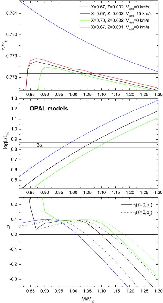
The top panel: the frequency ratio of the radial fundamental mode to the first overtone, ν1/ν2, as a function of a mass for models that fit the observed frequency ν1 = 18.19356 d−1. The models were computed with the OPAL opacity data. There is shown the effect of the initial hydrogen abundance (X0 = 0.67 versus 0.70), metallicity (Z = 0.002 versus 0.001), and rotation (Vrot, 0 = 0 versus 15 km s−1). The middle panel: the corresponding values of luminosity. The luminosities for non-rotating and rotating models overlap. The horizontal lines indicate the observed range of luminosity, as determined from the Gaia parallax, allowing for the 3σ error. The bottom panel: the corresponding values of the normalized instability parameter η. The solid lines correspond to the radial fundamental mode and the dashed ones to the first radial overtone. Modes with η > 0.0 are excited.
The first conclusion is that ν1/ν2(M) is not a monotonically decreasing function of a mass. As a consequence, there are two intersections with the line ν1/ν2 = 0.778192, corresponding to the observed value. The first intersection is for the mass of about M = 1.05 − 1.07 M⊙ and the second for M ≈ 0.85 − 0.87 M⊙. In all cases these low mass models have much too low luminosities. For lower metallicity Z = 0.001 and X0 = 0.67 the first intersection is for much higher mass M ≈ 1.31 M⊙ and luminosity log L/L⊙ ≈ 1.3, and the second one for much lower mass M < 0.8 M⊙ (not shown in the figure). Therefore we will not consider further this case.
As one can see from the top and middle panel of Fig. 2, only models computed with X0 = 0.67 and Z = 0.002 with masses of about |$M=1.05-1.07 \, \mathrm{M}_\odot$| are able to reproduce both the frequency ratio and luminosity. The model with |$M=1.05 \, \mathrm{M}_\odot$|, zero rotation and the parameters: log Teff = 3.8897, log L/L⊙ = 0.844, |$R=1.47 \, \mathrm{R}_\odot$| has the frequency ratio ν1/ν2 = 0.77818. The age of this model is about 2.84 Gyr, thus it is much younger than the one found by Petersen & Christensen-Dalsgaard (1996). This model ideally reproduces both the observed frequencies and parameters, but the star must rotate.
Including the initial rotation of Vrot, 0 = 15 km s−1 for the same chemical composition we got the seismic model with the parameters: |$M=1.073 \, \mathrm{M}_\odot$|, log Teff = 3.8969, log L/L⊙ = 0.878, |$R=1.48 \, \mathrm{R}_\odot$|, and ν1/ν2 = 0.77819. Thus, the model has the luminosity slightly above the 3σ error of the observed value of log L/L⊙. From the top panel of Fig. 2, we can see that decreasing the rotational velocity will shift the line ν1/ν2(M) down. We found that the model with a mass M = 1.055 M⊙ and Vrot, 0 = 10 km s−1 would reproduce, both, the two frequencies and stellar parameters. The effective temperature, luminosity, and radius of this model are log Teff = 3.8913, log L/L⊙ = 0.851, |$R=1.47 \, \mathrm{R}_\odot$| , respectively. The frequency ratio of the two first radial modes is ν1/ν2 = 0.77819. The current rotation is Vrot = 9.8 km s−1 and the age is 2.80 Gyr. The second intersection of the line ν1/ν2(M) with the observed frequency ratio occurs for the mass M = 0.838 M⊙ but the luminosity amounts only to about log L/L⊙ = 0.46.
For hydrogen abundance X0 = 0.70, metallicity Z = 0.002 and zero-rotation, the model with the mass M ≈ 1.02 M⊙ reproduces the two observed frequencies, but its luminosity is only log L/L⊙ = 0.721. Increasing the initial rotational velocity to 20 km s−1, we got the fit of the frequencies at the mass M = 1.082 M⊙, effective temperature log Teff = 3.8814, and the luminosity log L/L⊙ = 0.819, which is at the edge of the 3σ error. The model is 3.07 Gyr old. The rotation of this model is Vrot = 23.6 km s−1 and its radius |$R=1.48 \, \mathrm{R}_\odot$|. One more best seismic model from our search, which reproduces both the observed frequencies and luminosity of SX Phe, has the following parameters: X0 = 0.68, Z = 0.002, M = 1.06 M⊙, log Teff = 3.8867, log L/L⊙ = 0.834, |$R=1.47 \, \mathrm{R}_\odot$|, and the current rotation Vrot = 14.4 km s−1. The age of this model is about 2.92 Gyr.
The five seismic models described above, with corresponding evolutionary tracks, are depicted with dots in Fig. 3. All of them are in the post-main sequence phase and burn hydrogen in the shell. There are shown also the OP and OPLIB seismic models with corresponding evolutionary tracks. They will be discussed in the next subsection.
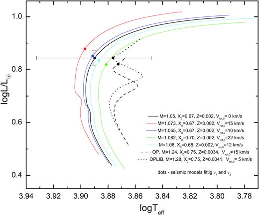
The HR diagram with the position of SX Phe and evolutionary tracks for various masses computed with the three opacity tables: OPAL, OP, and OPLIB. The tracks computed adopting the OPAL data are depicted with the solid line whereas those computed adopting the OP and OPLIB data with dashed and dotted line, respectively. The models that reproduce the observed frequencies of the two radial modes are marked with dots. The 3σ error was adopted for the Gaia luminosity. For the effective temperature the whole range available in the literature was included. Masses in the legend are in solar units.
The summary of the studied effects on the frequency ratio in the considered range of parameters is given in Table 2. The effect of overshooting from the convective core in the main sequence phase on the value of ν1/ν2 for models with M ≳ 1.1 M⊙ is negligible and we did not include it in our computations. For example, the difference in ν1/ν2 between the models with the overshooting parameter αov = 0.0 and αov = 0.2 is of the order of 10−5. Thus it is at the level of the numerical accuracy. Similarly, the value of the MLT parameter αMLT, describing the efficiency of non-adiabatic convection in the stellar envelope, has small effect on the frequency ratio. For example, the difference between the frequency ratio of models with masses around M = 1.05 M⊙ computed with αMLT = 0.0 and αMLT = 1.0 is of the order of 10−5.
The effect of various parameters on the frequency ratio of the radial fundamental mode to the first overtone for models appropriated for SX Phoenicis.
| The effect of X |
|---|
| X ↗ ⇒ |$\frac{\nu _1}{\nu _2}$| ↘ |
| The effect of Z |
| Z ↗ ⇒ |$\frac{\nu _1}{\nu _2}$| ↘ |
| The effect of Vrot |
| Vrot ↗ ⇒ |$\frac{\nu _1}{\nu _2}$| ↗ |
| The effect of αov |
| αov ↗ ⇒ |$\frac{\nu _1}{\nu _2}$| ↘ |
| The effect of αMLT |
| αMLT ↗ ⇒ |$\frac{\nu _1}{\nu _2}\approx {\rm const}$| |
It is quite probable that SX Phe itself is a blue straggler as many SX Phoenicis variables. Blue stragglers are presumably formed by the merger of two stars or by interactions in a binary system and, as a consequence, they may have enhanced helium abundance (e.g. McNamara 2011; Nemec et al. 2017).
Therefore, we consider models with a lower hydrogen (higher helium) abundance to be more preferred. These models rotate with the velocity of 10–15 km s−1. The projected rotational velocity of SX Phe is Vrotsin i = 18(2) km s−1, but most probably this value is overestimated because of a significant contribution of pulsation to the broadening of spectral lines. On the other hand, we cannot absolutely rule out the model with X0 = 0.70, Z = 0.002, M = 1.082 M⊙, log Teff = 3.8814, and log L/L⊙ = 0.819 (if we accept the 3σ error), rotating with the speed of 23.6 km s−1.
To fully accept the seismic model, we have to ask about excitation of the two first radial modes. In the bottom panel of Fig. 2, we plotted the instability parameter η for models considered in the two upper panels. The parameter η is a normalized work integral and it is greater than zero for unstable (excited) pulsational modes. The solid lines represent the fundamental mode whereas the dashed ones the first overtone. The values of η for non-rotating and rotating models overlap. The horizontal line indicates η = 0.0. As one can see, in the case of X0 = 0.67, Z = 0.002, the models with masses M < 1.1 M⊙ have both radial modes unstable. As for other seismic models described above, all of them have also both the radial fundamental as well as first overtone modes unstable.
2.3 The effect of opacity data
In the next step, we performed the same seismic modelling using stellar opacities from the OP and OPLIB projects. The results are presented in the same way as for the OPAL models in Figs 4 and 5. As one can see from the top panels, now the values of the frequency ratio ν1/ν2 of the models fitting the frequency ν1 are much higher than the observed value both for the OP models (Fig. 4) and for the OPLIB models (Fig. 5). Thus, in the allowed range of mass and luminosity, there is no model with the frequency ratio ν1/ν2 = 0.77819. The intersections occurring at |$M=0.81-0.87 \, \mathrm{M}_\odot$| have luminosities log L/L⊙ < 0.55. On the other hand, the models computed with the three sources of opacity data have very similar values of log L/L⊙ (cf. middle panels of Figs 2 , 4, and 5).
Considering what we have learned from seismic modelling of B-type stars (Daszyńska-Daszkiewicz et al. 2017; Walczak et al. 2019), this result is a bit surprising. In case of B-type pulsators with masses around |$8\!-\!12 \, \mathrm{M}_\odot$|, seismic models computed with OPAL and OPLIB data had similar parameters. In the case of SX Phe, the OP and OPLIB seismic models are rather similar.
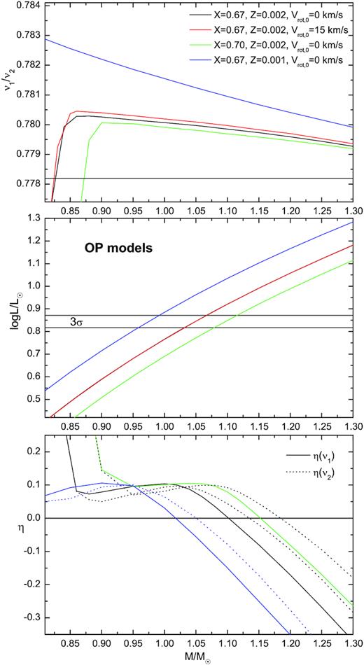
The same as in Fig. 2 but evolutionary models were computed adopting the OP opacities.
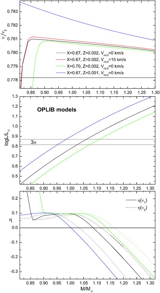
The same as in Fig. 2 but evolutionary models were computed adopting the OPLIB opacities.
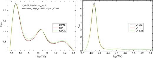
The left-hand panel: the run of the mean Rosseland opacity inside the models computed for the same parameters but with different opacity data: OPAL, OP, and OPLIB. The OPAL model reproduce the observed frequencies of the two radial modes of SX Phe as well as its effective temperature and Gaia luminosity. The model parameters are given in the legend. The right-hand panel: the corresponding values of the radiative gradient ∇rad.
Of course, the natural question arises: is it possible to achieve the fit of the two frequencies and luminosity with OP and OPLIB opacities by changing, in a reasonable range, such parameters as mass, hydrogen abundance, and metallicity?
The best fit with the OP data we obtained at the parameters: M = 1.24 M⊙, X0 = 0.75, Z = 0.0034, and Vrot = 17 km s−1. The radius of this model is slightly larger comparing to the radii of the OPAL seismic models and amounts to R = 1.55 R⊙. The logarithmic values of the effective temperature and luminosity are log Teff = 3.8725 and log L/L⊙ = 0.820, respectively. The age of this model is 2.62 Gyr. The position of the OP seismic model and the corresponding evolutionary track are shown on the HR diagram in Fig. 3. As one can see, the model is after an overall contraction, in the hydrogen shell-burning phase.
Similarly, using the OPLIB opacities, we had to increase significantly the initial hydrogen abundance and metallicity, up to X0 = 0.75, Z = 0.0041, respectively. The best OPLIB seismic model has the following parameters: M = 1.28 M⊙, |$R=1.56~\, \mathrm{R}_\odot$|log Teff = 3.8763 and log L/L⊙ = 0.845 and rotates with the velocity of Vrot = 5.5 km s−1. Its age is 2.31 Gyr. The position of the OPLIB seismic model and the corresponding evolutionary track are also shown on the HR diagram in Fig. 3. The model has just finished the overall contraction phase.
As one can see, the OP and OPLIB models have rather high metallicity and initial hydrogen abundance. Therefore, we consider these seismic models less probable but we cannot exclude them with 100 per cent certainty.
3 CONSTRAINTS FROM THE PARAMETER f AND INTRINSIC MODE AMPLITUDE ε
The method of mode identification described in Section 2.1, besides the mode degree ℓ, provides the semi-empirical values of the two complex quantities: the parameter f and the mode amplitude ε. The parameter f is the amplitude of the radiative flux variations at the level of the photosphere and ε give the relative radius variations. These two parameters are semi-empirical because their values depend on the model atmospheres, in particular, on the metallicity and microturbulent velocity ξt. However, for simplicity from now on, we will call the determined values of f and ε as ‘empirical’. To this aim we used the time-series multicolour photometry of Rolland et al. (1991).
As we mentioned, in Section 2.1, the diagnostic potential of this method is huge as a comparison of the theoretical and empirical values of f yields valuable constraints on parameters of the model and theory. In particular, for AF-pulsators, one can expect valuable constraints on the efficiency of convective transport in the outer layers.
3.1 The values of f and ε for models fitting the dominant frequency
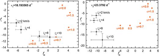
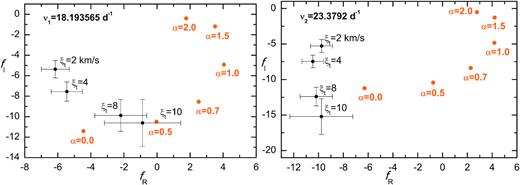
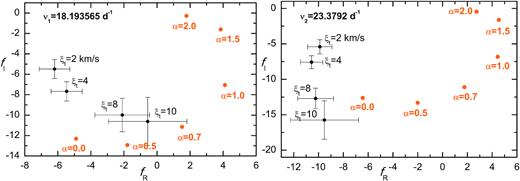
In Fig. 7, we show a comparison of the empirical and theoretical values of f as a function of a mass. All models reproduce the frequency ν1 = 18.193565 d−1 corresponding to the radial fundamental mode. The left-hand panels correspond to the dominant mode frequency ν1 = 18.193565 d−1 and the right-hand panels to the second frequency ν2 ≈ 23.38 d−1. In the top panels, a run of the real part of f is shown (fR) and in the bottom panels – the imaginary part of f (fI). Theoretical models were computed for the chemical composition X0 = 0.67, Z = 0.002, the OPAL opacities, and the five values of the mixing length parameter αMLT = 0.0, 0.5, 1.0, 1.5, 2.0. The rotation was not taken into account. The empirical values of f were derived adopting Vienna model atmospheres for the metallicity [m/H]= −1.0 and the four values of microturbulent velocity ξt = 2, 4, 8, 10 km s−1 . The model which fits the two observed frequencies has a mass |$M=1.05-1.06 \, \mathrm{M}_{\odot }$| as was described in Section 2.2. As one can see from the left-hand panels of Fig. 7, for the dominant frequency, also around this mass, we got the agreement between the theoretical and empirical values of f, simultaneous for the real and imaginary part, if the MLT parameter is below 1.0 and the microturbulent velocity is about 8 km s−1. Worse agreement was obtained for the second frequency ν2. In that case, for |$M\approx 1.05 \, \mathrm{M}_{\odot }$|, one can adjust the real part fR for αMLT < 0.5 and ξt ≈ 10 km s−1, whereas the imaginary part fI for αMLT < 1.0 and ξt ∈ (2, 4) km s−1. Nevertheless, the result is promising because the model reproduces two frequencies and the value of f for the dominant frequency, simultaneously. The best fit of the theoretical and observed amplitudes and phases is achieved for the model atmospheres with ξt = 4 km s−1. The results obtained for ξt = 10 km s−1 are rather excluded because the goodness of the fit, χ2, is about 3–4 times worse than those obtained with ξt = 4 km s−1. We will come back to the detailed comparison of the empirical and theoretical values of f for seismic models in the next subsection.
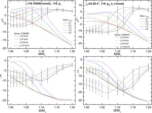
A comparison of the theoretical and empirical values of f in a function of a mass. All models fit the radial fundamental mode ν1 = 18.193565 d−1. The (semi)empirical values of f were determined from the Strömgren amplitudes and phases assuming the Vienna model atmospheres with different values of the microturbulent velocity ξt.
It is important to add that we cannot attach the above equation to the system of equations for the photometric amplitudes (equation 2) and derive simultaneously the parameters ε and f , because the time span between photometric and spectroscopic observations is too large. The Strömgren photometry was gathered in 1988 (Rolland et al. 1991) and the spectroscopy in 1976 (Kim et al. 1993). Thus, the phases of the light variations and radial velocity are not consistent. Nevertheless, it still makes sense to compare the values of the intrinsic amplitudes ε derived in Section 3.1 with the estimate from equation (12).
In Fig. 8, we plot the empirical values of |ε| as obtained from our method for models depicted in Fig. 7. As before, four values of the microturbulent velocity were considered ξt = 2, 4, 8, and 10 km s−1. The top and bottom panel corresponds to the first and second frequency, respectively. The horizontal lines mark the range of |ε| estimated from the amplitude of the radial velocity derived by Kim et al. (1993). As one can see, we got the agreement of |ε| between the values from our method and the estimates from AVrad for both frequencies simultaneously if the mass is less than about 1.15|$\, \mathrm{M}_{\odot }$| and the microturbulent velocity in the atmosphere is at least 4 km s−1. This result is in agreement with previous constraints derived from the parameter f. We can also tentatively say that the intrinsic amplitude of the radial fundamental mode of SX Phe is about six times the intrinsic amplitude of the radial first overtone mode.
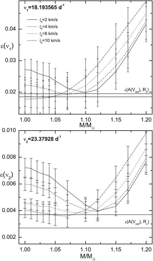
The empirical values of the intrinsic mode amplitude |ε| for models considered in Fig. 7. The top panel correspond to the dominant frequency (the radial fundamental mode) and the bottom panel to the second frequency (the first radial overtone). The horizontal lines mark the range of |ε(AVrad, R)| estimated from the radial velocity amplitudes and assuming the seismic radius |$R_{\rm s}=1.47 \, \mathrm{R}_\odot$|.
3.2 The values of f for models fitting the two frequencies: the effect of opacities
Now, we return to the parameter f and will make detailed comparisons of their empirical and theoretical values for seismic models described in Section 2. These models reproduce the two radial-mode frequencies and have the effective temperature and luminosity within the 3σ errors of the observed values. In Fig. 9, we show such comparison for the OPAL seismic model with the chemical composition X0 = 0.68, Z = 0.002, and the parameters: |$M=1.06 \, \mathrm{M}_\odot ,~\log T_{\rm eff}=3.8867,~\log \mathrm{L/L}_{\odot }=0.834,~R=1.47 \, \mathrm{R}_\odot$|. Its rotational velocity is 14.4 km s−1. The left-hand panel corresponds to the dominant frequency ν1 = 18.193565 d−1 and the right-hand panel to the second frequency ν2 = 23.37928 d−1. As one can see, for the dominant frequency we have the agreement between the empirical and theoretical values of f if the MLT parameter is in the range (0.5, 1.0) and ξt ∈ (8, 10) km s−1. The agreement for ξt = 8 km s−1 is marginal only if αMLT = 0.7. For the second frequency we could not match the empirical and theoretical values of f for any microturbulent velocity. The frequency ν2 has the photometric amplitude about three times smaller than the dominant frequencies. Thus, the amplitudes and phases of ν2 could be derived not enough precisely. Certainly, new photometric time-series observations made simultaneously with time-series spectroscopy, to include also the radial velocity into the method, could help settle this point.
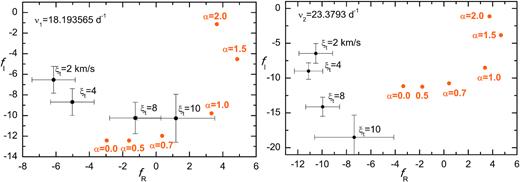
A comparison of the theoretical and empirical values of f on the complex plane for the radial fundamental mode (the left-hand panel) and for the first overtone mode (the right-hand panel). The theoretical values were computed for the OPAL seismic model with parameters: X0 = 0.68, Z = 0.002, |$M=1.06 \, \mathrm{M}_\odot ,~\log T_{\rm eff}=3.8867,~\log \mathrm{\mathit{ L}/L}_{\odot }=0.834,~R=1.47 \, \mathrm{R}_\odot$|, that rotates with the velocity of about 14 km s−1. The model is marked with a dot on the cyan evolutionary track in Fig. 3. Different values of the mixing length parameter αMLT were considered. The (semi)empirical counterparts were determined from the Strömgren photometry and the Vienna model atmospheres assuming different values of the microturbulent velocity ξt.
For the OPAL seismic model computed with the initial hydrogen abundance X0 = 0.67 the agreement is worse and only possible for the microturbulent velocity ξt = 10 km s−1. However, determinations of the empirical parameter f with ξt = 10 km s−1 have much worse goodness of the fit (2–4 times larger χ2 in equation 4) than for other values of ξt.
In Fig. 10, we compare the empirical and theoretical values of f for the OPAL seismic model with the chemical (X0 = 0.70, Z = 0.002 and the parameters: |$M=1.082 \, \mathrm{M}_\odot ,~\log T_{\rm eff}=3.8814,~\log \mathrm{\mathit{ L}/L}_{\odot }=0.819,~R=1.48 \, \mathrm{R}_\odot$|. Its rotational velocity is 23 km s−1. In this case, we got the solution for the empirical values of f determined with the microturbulent velocity ξt = 8 km s−1 and the theoretical values of f computed for the mixing length parameter αMLT ∈ (0.0, 0.5). As before, we excluded the solution with ξt = 10 km s−1 and αMLT = 0.7 because of much worse fit of the photometric amplitudes and phases.
The same comparison as in Fig. 9 but for the seismic OPAL model with parameters: X0 = 0.70, Z = 0.002, |$M=1.082 \, \mathrm{M}_\odot$|, log Teff = 3.8814, and log L/L⊙ = 0.819 (within the 3σ error), rotating with the velocity of 23.6 km s−1. The model is marked with a dot on the green evolutionary track in Fig. 3.
Again, for the second frequency, the empirical and theoretical values of f could not be reconciled for any value of αMLT and ξt.
The next two figures show comparisons of the theoretical and empirical values of f for seismic models found with the OP and OPLIB data; Figs 11 and 12, respectively. Quite surprisingly, these comparisons are qualitatively similar to the comparison for the OPAL seismic models (Figs 9 and 10), despite of significantly different masses and chemical composition. In the case of the OP seismic model, we can see that the theoretical and empirical values of f of the dominant mode agree if the mixing length parameter is in the range αMLT ∈ (0.0, 0.5) and the microturbulent velocity in the atmosphere is ξt = 8 km s−1. For the OPLIB seismic models, the matching for the dominant mode was possible for the range of about αMLT ∈ (0.5, 0.7) and only for ξt = 10 km s−1 .
The same comparison as in Fig. 9 but for the OP seismic model with parameters: X0 = 0.75, Z = 0.0034, |$M=1.24 \, \mathrm{M}_\odot$|, log Teff = 3.8725, and log L/L⊙ = 0.820 (within the 3σ error), |$R=1.55~\, \mathrm{R}_\odot$| and the rotational of 17 km s−1. The model is marked with a dot on the dashed evolutionary track in Fig. 3.
The same comparison as in Fig. 9 but for the OPLIB seismic model with parameters: X0 = 0.75, Z = 0.0041, |$M=1.28 \, \mathrm{M}_\odot$|, log Teff = 3.8763, and log L/L⊙ = 0.845, |$R=1.56~\, \mathrm{R}_\odot$| and the rotational velocity of 5.5 km s−1. The model is marked with a dot on the dotted evolutionary track in Fig. 3.
The first conclusion from Figs 9–12 is that, independently of the used opacity data and despite of different parameters of models, constraints on efficiency of the outer-layer convection is very similar. Namely, convection does not dominate the energy transport in the subphotospheric region and its efficiency is described by the mixing length parameter of about αMLT ∈ (0.0, 0.7).
The second conclusion is that, for the range of stellar parameters considered in this work, the parameter f is not a diagnostic tool for distinguishing between seismic models calculated with different opacity data.
4 SUMMARY
The goal of this paper was to construct seismic models of the star SX phoenicis that reproduce all observables that could be extracted from the available observational data. First, we made an independent mode identification from the photometric amplitudes and phases and confirmed pulsations of SX Phe in the two radial modes. Then, we search for models that fit the observed frequencies of the two radial modes adopting the three commonly used opacity data for evolutionary computations. The aim was to obtain models with the effective temperature and luminosity within the adopted observed errors. Besides, the requirement of instability of both pulsational modes must always be met.
The first result was that only with the OPAL data it was possible to construct such seismic models having a typical chemical composition for this prototype. Our best seismic OPAL models have the initial hydrogen abundance in the range X0 ∈ (0.67, 0.70) and metallicity Z = 0.002. Their masses are of about M = 1.05–1.08 M⊙, the radii: |$R=1.47-1.48~\, \mathrm{R}_\odot$| and the age: 2.80–3.07 Gyr. All seismic models are in the post-main sequence phase and burn hydrogen in the shell. The best seismic model of SX Phe found by Petersen & Christensen-Dalsgaard (1996) with the old OPAL opacities (Iglesias et al. 1992) had a mass M = 1.0 M⊙, metallicity Z = 0.001, initial hydrogen abundance X0 = 0.70, and the age 4.07 Gyr. Thus, it was much older than our best OPAL seismic models.
Then we searched for seismic models using OP and OPLIB opacity data. It appeared that in these cases, only models computed for significantly higher abundances of the initial hydrogen and metallicity are able to account for the two radial mode frequencies and have luminosity within the 3σ error. The OP seismic model have a mass M = 1.24 M⊙, radius |$R=1.55~\, \mathrm{R}_\odot$|, and the chemical composition X0 = 0.75, Z = 0.0034. It is after an overall contraction, in the hydrogen shell-burning phase, and its age is 2.62 Gyr. The OPLIB seismic model has similar parameters, namely: M = 1.28 M⊙, |$R=1.56~\, \mathrm{R}_\odot$|, X0 = 0.75, Z = 0.0041. The model has just finished the overall contraction phase and its age is 2.31 Gyr. However, we consider the OP and OPLIB seismic models as less reliable because of their high initial hydrogen abundance (X0 = 0.75) and metallicity (Z = 0.0034–0.0041). First, if SX Phoenicis would be a blue straggler, then it should have rather enhanced helium abundance (e.g. McNamara 2011; Nemec et al. 2017), hence lower hydrogen abundance. Secondly, the metallicity of the OP and OPLIB seismic models is higher than usually assumed for Population II stars. However, we currently do not have firm observables to rule out these models for certain.
In the next step, we used another seismic tool, that is the empirical values of the parameters ε and f derived from multicolour photometry. A comparison of the theoretical and empirical values of f for the dominant mode indicated low to moderately efficient convection, described by the mixing length parameter αMLT ∈ (0.0, 0.7). This conclusion is independent of the used opacity data, that is the same values of αMLT were estimated for seismic models computed with the OPAL, OP, and OPLIB tables. Moreover, this analysis showed that the microturbulent velocity in the atmosphere amounts to about ξt ∈ (4, 8) km s−1. Thus, despite a low mass of SX Phe (M ≈ 1.06–1.08 M⊙ for the OPAL seismic models), convective transport in its outer layers is not very efficient. This is because the radiative gradient is significantly reduced due to much lower opacity caused by very low metallicity.
The intrinsic mode amplitude, ε, of both frequencies derived from multicolour photometry are consistent with the values obtained from the radial velocity amplitudes. The relative radius variation for the radial fundamental mode is about 2 per cent and for the first overtone about 0.3 per cent.
Such comprehensive seismic studies of pulsators like SX phoenicis are very important for deriving constraints on convection in the outer layers, because the star is on the border between very efficient and inefficient convection. More stringent constraints from our complex seismic modelling could be derived for pulsators in double-lined eclipsing binaries. We plan to make such studies in the near future.
ACKNOWLEDGEMENTS
The work was financially supported by the Polish National Science Centre (NCN) grant 2018/29/B/ST9/02803.
DATA AVAILABILITY
Data on the photometric amplitudes and phases underlying this article are available in Rolland et al. (1991). Our theoretical computations will be shared on reasonable request to the corresponding author.
