


ABSTRACT
The fast folding algorithm (FFA) is a phase-coherent search technique for periodic signals. It has rarely been used in radio pulsar searches, having been historically supplanted by the less computationally expensive fast fourier transform (FFT) with incoherent harmonic summing (IHS). Here, we derive from first principles that an FFA search closely approaches the theoretical optimum sensitivity to all periodic signals; it is analytically shown to be significantly more sensitive than the standard FFT+IHS method, regardless of pulse period and duty cycle. A portion of the pulsar phase space has thus been systematically underexplored for decades; pulsar surveys aiming to fully sample the pulsar population should include an FFA search as part of their data analysis. We have developed an FFA software package, riptide, fast enough to process radio observations on a large scale; riptide has already discovered sources undetectable using existing FFT+IHS implementations. Our sensitivity comparison between search techniques also shows that a more realistic radiometer equation is needed, which includes an additional term: the search efficiency. We derive the theoretical efficiencies of both the FFA and the FFT+IHS methods and discuss how excluding this term has consequences for pulsar population synthesis studies.
1 INTRODUCTION
The standard search procedure for periodic pulsar signals relies on taking the fast fourier transform (FFT) of noisy input data and forming the fluctuation power spectrum (see e.g. Lorimer & Kramer 2004, for an overview). A sufficiently bright periodic signal manifests itself in the power spectrum as a discrete set of harmonics: peaks located at integer multiples of the signal’s fundamental frequency. The statistical significance of such a signal is evaluated by the sum of its normalized harmonic powers, a practice aptly named incoherent harmonic summing (IHS; Huguenin and Taylor, as described by Burns & Clark 1969). For each significant candidate thus identified, the original data are then phase-coherently folded modulo the candidate period to produce an integrated pulse profile and other diagnostic information that are then evaluated by a combination of visual inspection and, in more recent years, machine-learning algorithms (e.g. Lyon et al. 2016, for a review). The FFT has long dominated the landscape of pulsar searching, being the only periodicity search technique employed in nearly all major pulsar surveys of the past three decades (e.g. Johnston et al. 1992; Manchester et al. 2001; Cordes et al. 2006; Keith et al. 2010; Stovall et al. 2014).
However, an alternative method consists of directly folding the data at a wide range of narrowly spaced trial periods; the fast folding algorithm (FFA; Staelin 1969) does so efficiently by taking advantage of redundant operations. One integrated profile is produced for each trial period, which can then be evaluated for the presence of a pulse. Although as old as pulsar astronomy itself, for many years the FFA was rarely applied in practice and only for small-scale purposes. Examples include targeted searches of radio emission from X-ray emitting neutron stars (Crawford et al. 2009; Kondratiev et al. 2009), or attempts to find an underlying periodicity in the emission of the repeating fast radio burst FRB121102 (Scholz et al. 2016). Outside of pulsar astronomy, we may note that the FFA has been adapted to detect transiting exoplanets in Kepler photometry data (Petigura, Marcy & Howard 2013) and used in searches for extraterrestrial intelligence (SETI@home, e.g. Korpela et al. 2001). When it comes to large-scale FFA searches for pulsars, Faulkner et al. (2004) suggest that one was attempted for some time on the Parkes Multibeam Pulsar Survey (Manchester et al. 2001); they credited it with the discovery of a pulsar with a 7.7 s period, but there have been no subsequent publications on the matter. An interest in further developing the FFA has been growing in recent years; however, with the practical sensitivity analysis of Cameron et al. (2017) and the implementation of an FFA search pipeline on the PALFA survey by Parent et al. (2018) that has found a new pulsar missed by the standard FFT pipeline running on the same data.
So far, the FFA has been used mostly in niche cases because of its high computational cost (Lorimer & Kramer 2004; Cameron et al. 2017). The cost of an FFA search grows unreasonably large if one wants to probe shorter (P ≲ 500 ms) periods, and limited effort has been invested so far in making truly fast FFA implementations. On the other hand, highly optimized FFT libraries are widely available, upon which fast pulsar searching codes can be built. The FFT can also be efficiently extended to search for binary millisecond pulsars (e.g. Ransom, Eikenberry & Middleditch 2002). But sensitivity concerns have to be seriously taken into consideration.
Only one theoretical comparison between the sensitivity of the FFA and the standard FFT procedure has been published before (Kondratiev et al. 2009); its conclusion was that the FFA is better at detecting pulsars with both long periods (P ≳ 2 s) and short duty cycles (|$\delta \lesssim 1{{\ \rm per\ cent}}$|). More recently, a thorough analysis of the sensitivity of the PALFA pulsar survey (Lazarus et al. 2015) revealed that FFT searches do not reach their expected theoretical sensitivity to P ≥ 100 ms pulsars on real-world data, an effect that worsens for longer periods of a few seconds or more. The presence of low-frequency ‘red’ noise was found to be the main cause, and a suggested counter-measure was to use the FFA to search the long-period regime. Cameron et al. (2017) focused on the problem of assessing the output of the FFA for the presence of a pulsar signal; they empirically tested the behaviour of several pulse profile evaluation algorithms on a sample of real long-period pulsar observations. Methods based on matched filtering were found to perform better, and the FFA was shown to exceed the sensitivity of the FFT in a number of test cases. Parent et al. (2018) did a similar analysis on artificial data, and reported that on real PALFA survey data, their FFA implementation was on average more sensitive to pulsars with periods longer than a second (see their fig. 6) than the FFT-based presto pipeline (Ransom et al. 2002).
Although empirical sensitivity comparisons between search methods are important, it is not clear whether the differences in sensitivity thus measured between FFA and FFT search codes demonstrate an intrinsic superiority of either technique in a specific period or duty cycle regime, or if they are indirectly caused by technical implementation details. Particular concerns include how the statistical significance of signals is assessed, or the method used in FFT pipelines to mitigate the effects of low-frequency noise in Fourier spectra, which can have dramatic period-dependent effects (van Heerden, Karastergiou & Roberts 2017). To fully understand and then realize the true potential of the FFA, the intrinsic sensitivity of search methods must be compared analytically.
In this paper, we mathematically demonstrate that an FFA search procedure is more sensitive than its FFT counterpart to all periodic signals. In Section 2, we explain the FFA core operation, and propose a more computationally efficient variant of the original FFA algorithm. In Section 3, we formulate the general problem of detecting a signal in noisy data as a problem of statistical hypothesis testing; from there, we derive the optimally sensitive test statistic for the presence of a periodic signal in uncorrelated Gaussian noise, and show that calculating it amounts to running the FFA and convolving its output folded profiles with a matched filter. In Section 4, we use the same hypothesis-testing framework to calculate the sensitivity of the standard FFT+IHS method, and demonstrate that it is always outperformed by the FFA, moreso on smaller pulse duty cycles; pulse period is shown to be irrelevant in this comparison. In Section 5, we describe the details of our own FFA implementation riptide1 and how we propose to surmount the practical hurdles of realizing the full potential of the FFA on real data contaminated by low-frequency noise and interference. Our implementation is sufficiently fast to be employed on a modern all-sky survey. We discuss the implications of our results in Section 6. In particular, we caution that the radiometer equation of Dewey et al. (1985), if used to compute the minimum detectable flux density of a search, implicitly assumes that the method employed is phase-coherent and that the pulse shape is known a priori; we provide correction factors that more realistically account for the sensitivities of both the FFA and of the incoherent FFT-based standard method. We then conclude in Section 7.
2 THE FAST FOLDING ALGORITHM
The FFA is an efficient method to phase-coherently fold an evenly sampled time series at multiple closely spaced trial periods at once, taking advantage of the many redundant calculations in the process. It was originally devised to search for periodic signals in one of the very first pulsar surveys (Staelin 1969). In this section, we explain the principle of the FFA and describe a variant of the algorithm that produces identical results to the original, but does not require any input padding and uses modern CPU caches more efficiently.
2.1 The folding transform
If we consider an evenly sampled time series containing m cycles of a periodic pulsed signal with an integer period p (expressed in number of samples), the data may be represented as a two-dimensional array with m rows and p columns; each row represents an individual cycle, arranged in chronological order from top to bottom, and all pulses appear vertically aligned in phase. In this case, phase-coherently folding the signal is achieved by summing the array across all rows. However, if the period of the signal is increased to a larger, non-integer value p + Δp with 0 < Δp < 1, its consecutive pulses will appear to drift in phase towards higher values of pulse phase (i.e. the right-hand side), as illustrated in the example shown in the left-handl of Fig. 1. To phase-coherently integrate the signal, we now need to apply circular rotations to each pulse in order to compensate for the observed phase drift, which is a linear function of time; in other words, we must integrate the rows of the array along a diagonal path, whose slope can be defined by a single parameter s: the number of phase bins drifted towards the right between the first and last rows. Note that the integration path may wrap around in phase at the right edge of the array, possibly multiple times for higher values of s. The path s = 0 corresponds to a folding period of p, while s = m corresponds to a folding period of approximately p + 1. The exact relationship between s and folding period is derived in Section 2.3. We call the folding transform of the data the set of integrated pulse profiles obtained for all trial values of s with 0 ≤ s < m, which presents itself as an array of the same dimensions as the input data (right-handl of Fig. 1); column index represents phase, and each row corresponds to a trial folding period between p and approximately p + 1. Since the input data are discrete in time, integration paths with non-integer values of s are identical to that with the closest integer value, which means that the folding transform provides the highest possible period resolution for the given sampling rate. A brute-force calculation of the folding transform would take |$\mathcal {O}(p m^2)$| additions, but redundancies between consecutive period trials can be exploited.
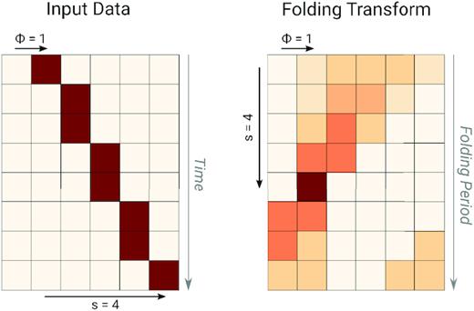
An illustration of the folding transform. Left-hand panel: input data, arranged in m = 8 rows of p = 6 samples, containing an artificial train of pulses with a width of one time sample, an initial phase of ϕ = 1 sample and a period larger than p, such that the pulses appear to drift in phase by s = 4 bins over the total observation time. Right-hand panel: folding transform of the input data, where darker colours denote larger integrated intensity. In a blind search, a visible peak in the folding transform denotes a candidate periodic signal; the row and column indices of the peak correspond to its period and initial phase, respectively.
2.2 A depth-first traversal, arbitrary length FFA
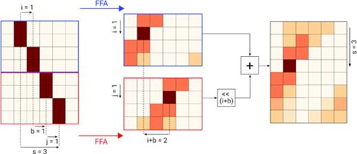
Depth-first variant of the FFA. The principle of the algorithm is to split the input data (left-hand panel) into two parts, outlined in blue and red, respectively, and independently calculate their folding transforms (middle panel); by adding together pairs of rows from each of these intermediate outputs with appropriate element-wise circular shifts, the folding transform of the whole input data (right-hand panel) can be obtained. It is shown in this specific example how the fourth row of the output, corresponding to an integration path with a total shift of s = 3 bins across the input data, is calculated. See text for a full explanation. This divide and conquer strategy is applied recursively, thus avoiding the redundant additions that would be performed in a brute force calculation of the folding transform.
The depth-first traversal FFA presented here is more efficient than the original breadth-first variant for two reasons. First, the depth-first variant can directly handle inputs with an arbitrary, non power-of-two number of rows m, removing the need to zero-pad the input data. This not only saves operations in the folding transform calculation itself, but also avoids creating additional folded profiles to be evaluated for the presence of a pulse. We note that the input data must still be presented in rectangular form, with a total number of samples that is a multiple of p. If the last input row is incomplete, it must be either ignored or padded to a full p samples; we have chosen the former option in our implementation because it is more computationally efficient. Secondly, a depth-first traversal of the tree has better memory locality and is more optimally suited to the hierarchical cache structure of modern CPUs: as the traversal proceeds towards the deeper layers of the tree, the calculations associated with a node and all of its sub-tree can fit entirely in cache once a certain depth is reached, regardless of the size of the full input. In contrast, the original breadth-first variant has to initially partition the input into two-row blocks and compute their respective transforms; for large inputs that cannot fit in the CPU cache, this requires two comparatively slow transactions with the main memory (RAM): one to read the entire input, another to write an equal-sized intermediate output with all two-row blocks transformed. All these operations have to be done before computing the next intermediate output with four-row blocks transformed. Building the final result in this order always requires a total of 2log2(m) RAM transactions, which negatively affects execution times.
2.3 Spacing of trial periods
3 OPTIMALLY SEARCHING FOR PERIODIC SIGNALS AND SENSITIVITY OF THE FFA
In this section, we examine the general problem of testing for the presence of a signal in discretely sampled noisy data, which is a matter of statistical hypothesis testing. After introducing all necessary technical terms, we find from first principles the optimally sensitive test statistic for detecting a signal with known parameters. For periodic signals, it emerges that computing this test statistic is equivalent to phase-coherently folding the data and correlating the output with a matched filter that reproduces the known pulse shape. In a practical search, the signal parameters are not known a priori; in this case a sensitivity penalty is incurred, which we quantify.
3.1 Problem formulation
H0: the data |$\mathbf {x}$| contain no signal, a = 0.
H1: the data |$\mathbf {x}$| contain the signal |$\mathbf {s}$|, a > 0.
To that end, we need a mathematical function |$T(\mathbf {x})$|, a test statistic, that reduces the data |$\mathbf {x}$| to a single summary value from which one can sensibly decide between hypotheses. For any test statistic, one must also define a so-called critical region, which is the set of values of |$T(\mathbf {x})$| for which the null hypothesis is rejected. In most practical applications, as will be the case here, the critical region will simply be defined by a threshold above which (or below which) one decides in favour of H1. Here, we want to find a test statistic (and critical threshold) that maximizes the sensitivity of our search for the presence of |$\mathbf {s}$|, a concept that first needs to be rigorously defined.
3.2 Evaluating a test statistic
When choosing between hypotheses, two types of errors can be made. A type I error is a rejection of the null hypothesis H0 when it is true, which in pulsar astronomy parlance is a false alarm or false positive. A type II error is a rejection of the alternative hypothesis H1 when it is true − here, quite simply a missed pulsar. Unless the decision problem is trivial, there is no perfectly accurate test, so that there exists a trade-off between the two types of error rates; when evaluating tests, the standard practice is therefore to first set an acceptable false positive rate, or significance level noted α, and identify which test exhibits the lowest type II error rate while maintaining a type I error probability smaller than α (e.g. Casella & Berger 2002). For our specific purposes, the sensitivity of a test statistic T to a given signal shape |$\mathbf {s}$| can be rigorously evaluated by following the procedure below:
Set the significance level α. In a pulsar search, the choice of α is usually made so that no more than one false alarm per observation occurs on average, assuming ideal data without interference signals (e.g. Lorimer & Kramer 2004).
- Calculate the critical threshold η of the test statistic T associated with the chosen false alarm rate α. η is defined bywhere the notation P(E|H) denotes the probability of event E given hypothesis H is true.(9)$$\begin{eqnarray*} P(T(\mathbf {x}) \ge \eta | H_0) = \alpha , \end{eqnarray*}$$
- Assuming the alternative hypothesis H1 is true, compute the probability γ that T exceeds the critical value:γ is called the statistical power of the test T, or completeness of the search, and it is a function of the signal amplitude a.(10)$$\begin{eqnarray*} P(T(\mathbf {x}) \ge \eta | H_1) = \gamma (a). \end{eqnarray*}$$
3.3 Constructing the most powerful test: the Z-statistic
Choose H1 if |$Z(\mathbf {x}) \ge \eta _z(\alpha)$|.
Choose H0 otherwise.
3.4 Case of periodic signals
3.5 Searching for periodic signals with unknown parameters
Their period p.
Their pulse phase ϕ at the start of the observation.
Their duty cycle δ, defined as the ratio between pulse width and period.
4 SENSITIVITY ANALYSIS OF THE STANDARD FFT PROCEDURE
After establishing the optimal, or near-optimal sensitivity of an FFA search procedure, we now need to quantify how the standard incoherent FFT-based search performs in comparison. Although the topic of the sensitivity of a sum of Fourier harmonics to periodic signals has been covered before (e.g. Groth 1975; Vaughan et al. 1994; Ransom et al. 2002; Kondratiev et al. 2009), we will do so again in a way that fits the hypothesis testing framework laid out in the previous section. This will allow a mathematically rigorous comparison of FFA and FFT upper limits.
4.1 The incoherent detection statistic
4.2 Distribution of the incoherent detection statistic
4.3 Statistical power analysis
The pulse shape, which defines the cumulative harmonic power distribution P(h): to remain consistent with the analysis done on the FFA above we also use Gaussians, parametrized by their full-width at half-maximum (FWHM) in units of pulse period
The significance level, that we set to 7σ, i.e. |$\alpha = \bar{\Phi }(7)$| where |$\bar{\Phi }$| is the survival function of the normal distribution.
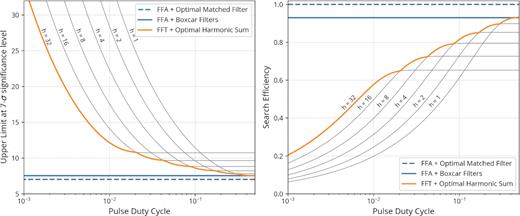
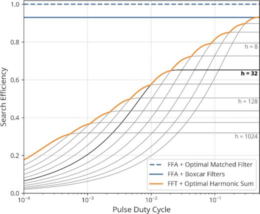
Sensitivity comparison between an FFA-based search and the standard FFT procedure with incoherent harmonic summing. We assumed a significance threshold of 7σ and a periodic signal with a Gaussian pulse shape. Left-hand panel: upper limit as a function of Gaussian pulse FWHM (in log-scale), expressed in units of pulse period. The upper limit of a search procedure is the minimum signal amplitude (in units of background noise standard deviation) that it can detect with 50 per cent probability. See Section 3.1 for a rigorous definition of amplitude. The theoretical optimum upper limit (|$\mathcal {U}_z = 7$| here) could be achieved by the FFA if the pulse shape and width were known a priori (blue dashed line); in practice, a penalty is incurred when using boxcar matched filters (blue solid line). FFT search codes compute multiple harmonic sums, typically up to 32 harmonics, whose individual upper limits are plotted as grey curves; the upper limit of the whole FFT procedure corresponds to their lower envelope (orange line). Right-hand panel: search efficiency |$\mathcal {E}$|, i.e. ratio between the theoretical optimum upper limit |$\mathcal {U}_z$| and the upper limit of each search procedure. |$\mathcal {E}_\mathrm{FFA} \approx 0.93$| in practice. It is implicitly assumed that the FFA search employs enough output phase bins to resolve the pulse.
We note that some past surveys (e.g. Manchester et al. 2001) have used the phase information of the harmonics of candidates reported by the incoherent harmonic sums to reconstruct their integrated pulse profile, and also estimate their phase-coherent S/N. Although this process is useful in removing chance detections, it does not change the upper limit of the search as a whole for a fixed false alarm probability α, because it can only be applied to signals bright enough to exceed the detection threshold of the FFT+IHS procedure in the first place. Computing resources permitting, implementing this second-stage selection process might however justify an increase of the acceptable α for the FFT+IHS procedure in practice.
4.4 Summary
We have rigorously shown that in the presence of pure uncorrelated Gaussian noise, a phase-coherent FFA-based search is more sensitive than the incoherent FFT search procedure regardless of pulse period and duty cycle. The improvement offered by the FFA is greater for shorter pulse duty cycles. We do note, however, that there may be some exotic pulse shapes for which the standard FFT procedure can still outperform the FFA in terms of sensitivity, if the set of matched filters used in the FFA search does not account for their possible existence. For example, a pulse with two widely spaced identical peaks may see only one of them matched by a set of single-peaked matched filters, resulting in at best |$\approx 71{{\ \rm per\ cent}}$| efficiency.3 In that sense, the incoherent harmonic sum could be said to be more agnostic to pulse shape. On the other hand, we have assumed that the fundamental signal frequency falls at the centre of a Fourier frequency bin, i.e. it is an integer multiple of 1/N. This corresponds to the best-case sensitivity scenario for the FFT method, where all of the signal power is concentrated in Fourier bins with frequencies that are multiples of the fundamental. Otherwise, a significant amount of power leaks to neighbouring bins, a sensitivity-reducing effect known as scalloping; it can in principle be eliminated using so-called Fourier interpolation, but not entirely so in practice due to limited computing resources (see section 4.1 of Ransom et al. 2002, for details). In large-scale searches, a computationally cheap version of Fourier interpolation called interbinning is employed, that results in a worst-case loss of SNR of 7.4 per cent, which is equivalent to further dividing the FFT’s search efficiency by 1.074.
5 AN IMPLEMENTATION OF THE FFA TO PROCESS LARGE-SCALE PULSAR SURVEYS
Implementing an FFA search pipeline that conserves all its desirable properties on ideal data when faced with real-world, imperfect data are challenging. In this section, we will describe all the practical problems that need to be surmounted, the proposed solutions that we implemented in our own FFA search software package riptide, and a rationale behind the technical choices that we made. A significant amount of practical knowledge was gained by testing and refining the implementation on a portion of the SUPERB survey (Keane et al. 2018), in particular on observations of known sources that were either faint or made difficult to detect by different strains of radio-frequency interference.
5.1 Overview of the implementation
The high-level interface of riptide is written in the python language, while the performance-critical sections of the code are implemented in optimized c functions. riptide provides a library of python functions and classes that can be used to perform interactive analysis and visualisation of dedispersed time series data, using for example ipython or jupyter. The high-level functions of riptide form the building blocks of its pipeline executable, that takes a set of dedispersed time series as input and outputs a number of data products, including a set of files containing the parameters of detected candidate signals and useful diagnostic information (see Section 5.7 for details on the pipeline itself). The code is modular so that it can in principle support arbitrary data formats; currently, riptide can process dedispersed time series files produced by either presto4 (Ransom et al. 2002) or sigproc5 (Lorimer 2011) pulsar software packages.
5.2 Data whitening and normalization
In Section 3, we have demonstrated the optimal sensitivity of the combination of the FFA and matched filtering, but under the significant assumption that the background noise was Gaussian with mean m and standard deviation σ known a priori, that we took to be 0 and 1, respectively, without loss of generality. In practice these parameters have to be estimated from the data directly, in the presence of an additional low-frequency noise component and possibly interference. Devising an efficient and unbiased estimator for m and σ in the general case is extremely challenging, as it would require fitting the low-frequency noise component parameters, any detectable signal regardless of its nature, and m and σ simultaneously. To that we must further add the constraint that evaluating the noise parameters should be done in a small fraction of the time taken by the search process.
Cameron et al. (2017) have partially avoided this problem by essentially evaluating m and σ in every folded profile separately, using its so-called baseline, a region of the pulse that appears to contain no signal defined by empirical criteria. This method has long been employed in pulsar search and timing software, and is implemented for example in the widely used psrchive package (Hotan, van Straten & Manchester 2004). However, doing so has a number of drawbacks. In particular, the estimators for the noise parameters have to work with a small number of data points, no larger than the number of phase bins, yielding uncertain estimates that significantly vary from one pulse to the other, and in turn increase the uncertainty of the output S/N values. At longer trial periods, the baseline is also more likely to be contaminated by low-frequency noise. Furthermore, and most importantly, any procedural method to locate the baseline region needs to use criteria such as excluding a putative pulse even where there is none present (e.g. ‘Algorithm 2’ in Cameron et al. 2017), or search for a contiguous segment of the profile with the lowest mean (implemented in the pdmp utility of psrchive). The two methods above yield estimates of m and σ that are systematically biased low in the presence of pure noise, and therefore S/N values that are biased high, which invalidates the optimal sensitivity demonstration made in Section 3.
Our priority was therefore to remain within all mathematical assumptions of Section 3, at least to the extent allowed by real-world data. We have chosen to directly evaluate the noise parameters from the whole input time series once during pre-processing, in an attempt to obtain unbiased and low-variance estimates. This approach is also used by Parent et al. (2018). In our implementation, we first remove the low-frequency noise component by subtracting a running median from the input data; the width of the median window is left to the user to choose and optimize. The running median filter has the desirable property of leaving intact any constant impulse whose width is less than half that of the window (Gallagher & Wise 1981). Then the input time series is normalized to zero mean and unit standard deviation before being searched.
5.3 Searching a period range
A given period range [P0, P1] could naively be searched by calculating a sequence of folding transforms, with base periods (and therefore number of output phase bins) expressed in number of samples ranging from p0 = ⌊P0/τ⌋ to p1 = ⌈P1/τ⌉, where τ is the time resolution of the input data, |$\lfloor \, \rfloor$| and |$\lceil \, \rceil$| are the floor and ceiling functions, respectively. However, if P1/P0 ≫ 1 this procedure has a highly non-uniform phase and pulse duty cycle resolution, which can become excessively high at trial periods of a few seconds and higher, especially in an era where τ is typically on order of tens of microseconds. The standard way to circumvent the problem, adopted by previous FFA implementations (Kondratiev et al. 2009; Cameron et al. 2017), is to iteratively downsample the input data by a factor of two, and consecutively search so-called octaves of the form [2kP0, 2k + 1P0], where within each octave the number of phase bins in the output folded profiles increases from b to 2b proportionally to the trial period, with b being a user-defined parameter that sets the minimum duty cycle resolution. We have implemented the same procedure in riptide, with one difference worth mentioning: we have provided the option to use real-valued, strictly smaller than 2 downsampling factors which generates more numerous and shorter pseudo-octaves. In practice, the user chooses a minimum and maximum number of output of phase bins bmin and bmax, respectively, and the data are iteratively downsampled by f = (bmax + 1)/bmin rather than f = 2. We have made this choice both to maintain the duty cycle resolution much closer to uniform, rather than let it oscillate by a factor of two; furthermore, if what matters most when reporting on a large-scale FFA search is the lowest duty cycle resolution across the period range explored, then one should attempt to increase the minimum number of phase bins while maintaining the maximum number of phase bins as low as possible to avoid spending additional computing resources. The whole search process is summarized as a diagram in Fig. 4.
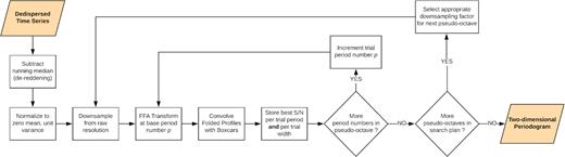
Sequence of operations performed by riptide when processing a dedispersed time series over a user-defined period range, see also Section 5.3 for a detailed explanation. The output periodogram is two-dimensional as the code returns the highest S/N per period trial and per pulse width trial, rather than just the best S/N per period trial across all pulse widths. In practice this can greatly improve sensitivity to narrow pulses in the presence of interference or low-frequency noise (see text and Fig. 5).
There are a few of details to be aware of here, firstly that using a non-integer factor makes any two consecutive samples in the downsampled data correlated with each other. This is not a problem in principle because when folding, the samples integrated in any given phase bin are not consecutive and therefore uncorrelated. But this may not be the case anymore if chaining (i.e. composing) many downsampling operations, which we carefully avoid doing in our implementation. When moving from one pseudo-octave to the next, we always return to the original highest resolution data, and downsample it with the appropriately chosen, geometrically increasing factor. The real caveat actually lies in how downsampling by a real-valued factor f affects the noise variance in the output samples. If the input data are uncorrelated Gaussian noise with unit variance, then the sample variance of the output data is |$f - \frac{1}{3}$| rather than f as one would expect when using an integer factor. This is shown in Section A4 and properly accounted for in riptide.
5.4 Matched filtering
5.5 Identifying statistically significant candidate signals
Overall the combination of FFA and matched filtering returns S/N as a function of trial period, width, and phase, which can be too large to be fully kept in memory especially when processing multiple dispersion measure (DM) trials. FFA implementations typically reduce this output to a so-called periodogram, a one-dimensional array containing the highest S/N as a function of trial period (across all possible trial widths and phases). On ideal data containing only uncorrelated Gaussian noise and a possible periodic signal, identifying statistically significant signal periods is a trivial exercise of applying a threshold to the periodogram; the threshold value is the critical value of the z-statistic (equation 16), i.e. the number of Gaussian sigmas that correspond to the desired false alarm probability. However, situations where this is not applicable arise relatively often in practice. If the data are contaminated by low-frequency noise, then it will manifest itself in every folded profile at longer trial periods (typically a few seconds) in the form of a fluctuating baseline, to which the widest matched filters have optimal response. Randomly occurring bursts of interference are also empirically found to have a similar effect. We have noticed on several Parkes L-band test cases that keeping in memory only the best S/N value across all trial widths runs the risk of missing long period pulsar signals that could otherwise be found in a blind search. This is illustrated in Fig. 5 on a Parkes multibeam observation of the 12.1-s pulsar PSR J2251–3711 (Morello et al. 2020) affected by interference: the pulsar emerges as a clear peak if considering the optimal trial width in isolation, but is undetectable if the only information available is the best S/N versus period plot. We therefore keep in memory the highest S/N as a function of both trial period and width, making the output periodograms of riptide two-dimensional; each pulse width trial is then post-processed separately.
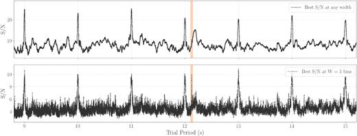
Highlighting the advantages of analysing pulse width trials separately when searching for long-period faint sources. Here, we have run riptide on a 9-min Parkes L-band observation of PSR J2251–3711, dedispersed at the known DM of the pulsar. The 12.1-s period of the pulsar is highlighted in orange; many harmonics of an interference source with a 1-s period are detected. Top panel: best S/N obtained across all trial pulse widths as a function of trial period. For most trial periods, the highest S/N is obtained with the widest matched filter due to its optimal response to residual low-frequency noise, and the peak associated with the pulsar is difficult to distinguish from the background. Bottom panel: S/N obtained specifically with the optimal 3-bin width matched filter, where the associated peak could be identified in a blind search. |$\rm{\small RIPTIDE}$| keeps one periodogram per width trial in memory which are then independently searched for peaks, in an attempt to be robust to situations with imperfect data.
Furthermore, periodograms of contaminated data commonly show a trend of S/N increasing as a function of period, and all reported S/N values above a certain trial period may exceed the theoretical significance threshold. Whether or not a peak is significant can then only be evaluated relative to neighbouring period trials; visual inspection of periodograms is not an option in a large-scale survey, and a reliable peak identification algorithm is required. This is a crucial part of a pipeline, which if not carefully designed can vastly reduce the inherent sensitivity of the FFA itself in many imperfect data situations; it should also run in a reasonable fraction of the time required by the computation of the periodogram itself. Our peak finding algorithm is based on evaluating, as a function of trial period, the overall trend of the S/N and the dispersion around it (Fig. 6), in order to determine how far above the trend a point should lie to be considered significant. We first divide the whole trial frequency range into equal-sized segments. Here, we operate on trial frequency rather than trial period, basing ourselves on the property that the complex-valued coefficients of the DFT of uncorrelated Gaussian noise are also uncorrelated; the DFT frequency bins are spaced by 1/T where T is the integration time, and one can expect the S/N values in an FFA periodogram to decorrelate on a frequency scale on order of 1/T as well. The width of the frequency segments is thus chosen to be Δzseg/T where Δzseg is a dimensionless free parameter. In each segment, we calculate the median m of the S/N values and estimate their standard deviation σ from the interquartile range (IQR) of the S/N values using σ = IQR/1.349, in order to be robust to outliers. An estimate of the local significance threshold is s = m + kσ where k is a dimensionless parameter defining the significance level. All segments thus provide a set of control points (νi, si) where νi is the centre frequency of the i-th segment and si the estimated local significance threshold. The last step is to fit a function of frequency to this set of points. Here, the choice of functional form might aim to reflect that the data are expected to contain two noise components: a Gaussian component with uniform power as a function of frequency, and a low-frequency component whose power is typically modelled as proportional to ν−α where α > 0 is the noise spectral index (α = 2 in the case of Brownian noise). With signal power being the square of S/N, a logical choice appears to be a function of the form |$s = \sqrt{A \nu ^{-\alpha } + B}$|; however, we found that it often yields a poor fit to the control points on real test cases, by overestimating the selection threshold at low frequencies. We attribute this to the red noise reduction effect of the running median filter and the presence of interference. Furthermore, this fit is non-linear and does not converge all the time, which is highly undesirable as we aim for maximum reliability. In the end, we found that the best results were obtained with a polynomial in log (ν), a function that does not diverge around ν = 0 and can be reliably fit with the linear least-squares method. The degree of the polynomial is exposed as a free parameter, and is equal to 2 by default.
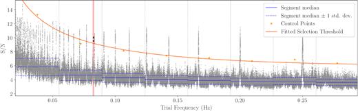
An explanation of the peak detection algorithm employed in riptide, using the same observation of PSR J2251–3711 as in Fig. 5. For each individual trial width, the S/N versus trial frequency array is partitioned into equal-sized frequency segments with a width of a few times 1/T where T is the length of the input time series. Within every segment, the median m and standard deviation σ of the S/N are calculated using robust estimators. Each segment yields a control point with coordinates (ν, s), where ν corresponds to the centre frequency of the segment and s = m + kσ where k is a parameter set to k = 6 by default. Finally, a second-degree polynomial in log (ν) is fitted to the control points, yielding the peak selection threshold (orange line). Any points lying above the threshold are clustered into peaks. The detection of the pulsar is highlighted with a red background and bolder points. See text for full details and the design rationale for this algorithm. Note that the frequency segments are much narrower in practice, they have been widened here for readability.
We can note that the exact same candidate selection problems caused by S/N trends are encountered in FFT-based periodicity searches as well, where the low-frequency bins of Fourier spectra contain significant excess power. The classical solution in FFT search implementations is to perform so-called ‘spectral whitening’, where portions of the power spectra are divided by a factor dependent on the locally estimated power average (Israel & Stella 1996; Ransom et al. 2002). Our dynamic thresholding algorithm above is conceptually similar.
5.6 Improving performance with dynamic duty cycle resolution
5.7 Full pipeline overview
In a large-scale pulsar survey processing scenario, an FFT-based search that would be running simultaneously already requires an observation to be dedispersed into a set of time series each with their trial dispersion measure, with a DM step almost certainly finer than required by an FFA search. The riptide pipeline is designed to take advantage of this situation, taking a set of existing DM trials as an input and processing only the minimal subset necessary to achieve adequate DM space coverage; the trial DM step is chosen using the classical method, that is based on limiting the pulse broadening time-scale due to dedispersing the data at a DM different from that of the source (e.g. chapter 6 of Lorimer & Kramer 2004). If running riptide on its own, then the user is responsible for dedispersing the data with the appropriate DM step beforehand. All selected DM trials are then distributed between available CPUs using the multiprocessing standard library of python, and processed in parallel. For each DM trial a periodogram is produced and searched for peaks, but only the peak parameters are accumulated in memory. Once all time series have been processed, the parallel section of the pipeline ends. All reported peaks are then grouped into clusters in frequency space, and clusters that are harmonics of others are flagged. The user decides whether such harmonics are kept and later output as candidates, or discarded immediately; finally, for each remaining cluster, a candidate object is produced. The code saves the following data products:
A table of all detected peak parameters before clustering. These include: period, DM, width in phase bins, duty cycle, S/N.
A table of cluster parameters, with any harmonic relationships. The cluster parameters are simply that of its brightest member peak object.
Candidate files in JSON format each containing: a list of best-fitting parameters (period, DM, S/N, duty cycle), a subintegrations plot produced by folding the de-reddened and normalized time series associated with the best-fitting DM, all available metadata of the observation (e.g. coordinates, integration time, observing frequency, etc.), and a table of all detected peaks associated with the candidate.
Candidate plots, although this can be disabled to save time; plots can still be produced later.
Saving intermediate data products enables one to test all post-processing steps on known pulsar observations, and further improve them in the future. It is important to verify for example if a known pulsar is missed because it is genuinely undetectable, or if it registers as a peak and then is lost due to erroneous clustering or harmonic flagging.
5.8 Benchmarks
To measure the speed of the riptide pipeline, we have decided to avoid using a pulsar observation, because the total number of candidate files that must be produced by the final stage of the pipeline is dependent on the signal content of the data. For reproducibility purposes, we have therefore measured the execution time of the riptide pipeline (version 0.1.0) on a set of 128 DM trials made of artificially generated Gaussian noise. Each time series was 9 min long, containing 223 time samples with a 64 µs sampling interval, reproducing the parameters of recent Parkes multibeam receiver surveys (Keith et al. 2010; Keane et al. 2018). The benchmark was conducted on a node of the OzStar computing facility, reserving 16 Intel Gold 6140 @ 2.3GHz CPU cores to search the data in parallel. Here, we deliberately did not use the dynamic duty cycle resolution feature previously described, choosing instead to specify a single, wide period search range with the same bmin and bmax parameters in order to keep the experiment simple. We provided riptide with the following base configuration:
Minimum search period Pmin = 1.0 s.
Maximum search period Pmin = 120.0 s.
Average number of phase bins bavg = 1024, for a duty cycle resolution of |$\delta = 0.1{{\ \rm per\ cent}}$|. In practice we specified the code parameters bmax and bmin to be equal to bavg plus and minus 4 per cent, respectively.
Nproc = 16 parallel processes, one per available CPU core.
We then measured how individually changing the parameters Pmin, bavg, and Nproc (while keeping all other parameters fixed) affected the total processing time per DM trial. The results are shown in Fig. 7. The execution times as a function of minimum trial period and number of phase bins are well predicted by the asymptotic complexity expression given in equation (40). A deviation from the prediction is observed where the search is computationally cheap, that is for both lower number of phase bins and higher minimum trial periods: in this regime, the total execution time is instead dominated by the overheads of reading, de-reddening and normalizing the input data. However, the performance of the pipeline was not found to scale quite linearly with the number of CPUs employed; although some operations of the pipeline run sequentially and do not benefit from multiple CPUs, we found that the non-parallel sections of the code consumed a negligible amount of time in this experiment. We therefore attribute the observed effect to limited memory bandwidth, for which multiple CPUs likely compete. Overall, a single 9-min DM trial can be processed in approximately one second on a modern compute node with 16 CPU cores, while using at least 1000 phase bins for trial periods of a second or longer.
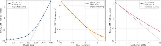
Processing time per DM trial of the riptide pipeline, evaluated on a set of 128 artificial DM trials with a length of 9 min and a sampling time of 64 µs. The pipeline was initially configured to search trial periods from 1 to 120 s with 1024 phase bins, and allowed to use 16 CPU cores. We then measured how changing one configuration parameter at a time from this initial setup affected the execution time. The plots show the total processing time per DM trial as a function of the average number of output phase bins (left), minimum trial period (middle), and number of CPU cores (right). For the left and middle plots, the expected scaling is extrapolated from the most intensive test case (i.e. with the highest run time) using equation (40), which gives the asymptotic complexity of searching a single time series. For the right plot, the expected scaling is a linear performance increase as a function of number of CPU cores. See text for more details on the experimental setup and a discussion of the results.
6 DISCUSSION
6.1 A more realistic radiometer equation to determine detectable flux densities
Above and beyond assessing the detection efficiency, a further caveat is needed when using values calculated by equation (43) to infer intrinsic pulsar properties. It would be incorrect to interpret flux density values determined in this way, that apply to detection thresholds in the final dedispersed data stream, as simply scaled versions of intrinsic pulsar properties. For example it is common to scale up flux densities determined from the (even uncorrected) radiometer equation by the square of the distance to a pulsar to infer an intrinsic property. When doing this, at the very least an extra efficiency factor should come into play to account for the various transfer functions of the interstellar medium, telescope system, dedispersion procedures, etc., and in reality the inversion might be quite complex and line-of-sight dependent. The end result, as to what fraction of the intrinsic population is probed by these searches, contains this difficult-to-account-for incompleteness.
6.2 Improving FFT searches with coherent harmonic summing
Same search efficiency plot as in Fig. 3, also assuming a 7σ significance level and a Gaussian pulse, except that we have allowed for the incoherent summation of up to 1024 harmonics. We have extended the X-axis to include pulse duty cycles down to 0.01 per cent. The usual limit of 32 harmonics summed in most search codes is highlighted in black. Summing more harmonics is beneficial for duty cycles shorter than about 1 per cent, but cannot compensate for the lack of phase-coherence of this search procedure.
6.3 Efficacy of the FFA in a real search
We have covered in-depth the topic of the theoretical sensitivity of the FFA, but its ability to discover new pulsars in practice is of high importance. riptide has successfully been used to discover new pulsars that were missed by FFT search codes running on the same data. An early development version of riptide was used to process a portion of the SUPERB survey (Keane et al. 2018). This search was highly experimental for several reasons; the pipeline used a crude peak detection algorithm to analyse periodograms which may have resulted in missed detections, and employed a low number of phase bins (250) even at the longest search periods which clearly limited its ability to find short duty cycle pulsars similar to the 23.5-s PSR J0250+5854 (Tan et al. 2018). Furthermore, the accuracy of the candidate selection algorithm employed was limited compared to the one running on the candidates produced by the standard FFT search. In spite of these limitations, 9 previously unknown pulsars missed in the FFT analysis were discovered, with periods ranging from 373 ms to 2.4 s and duty cycles larger than one per cent. Timing solutions for these discoveries are presented in Spiewak et al. (2020). A new, deeper FFA search of the entire SUPERB survey and of several other Parkes archival surveys will be performed soon (Morello et al., in preparation).
More recently, riptide has been used to discover the previously unknown pulsar PSR J0043–73, with a 937 ms period, in a deep targeted search of the Small Magellanic Cloud (Titus et al. 2019). This source was not detected by the FFT-based presto running on the same data, although it should be noted that to save computing time, it was only allowed to sum up to 8 harmonics. In the same data, the known pulsar PSR J0131–7310, with a 348-ms period, was also detected exclusively by riptide. Furthermore, a complete re-processing of the LOFAR Tied-Array All-Sky Survey (Sanidas et al. 2019) is currently in progress where riptide is being run in parallel to presto. The results will be reported in a future paper (Bezuidenhout et al., in preparation).
The fact that riptide has discovered a number of pulsars with relatively short periods (less than a second), in a regime where the FFA was previously thought to bring no substantial benefits, is both encouraging and consistent with the theoretical sensitivity analysis presented here. Any difference in the number of pulsars detected between FFA and FFT search codes may result not only from the higher intrinsic sensitivity of the FFA, that we have demonstrated in this paper, but also from other implementation details such as low-frequency noise and interference mitigation schemes, which may be of equal if not higher importance. A thorough empirical comparison between riptide and other FFT search codes (presto in particular) on real data will be performed in the aforementioned upcoming publications.
7 CONCLUSION
We have analytically shown that a search procedure that combines a FFA with matched filtering is optimally sensitive to periodic signals in the presence of uncorrelated Gaussian noise. In particular it is more sensitive than the standard FFT technique with incoherent harmonic summing to all periodic signals. We have defined a search efficiency term, to rigorously compare the sensitivities of pulsar searching procedures; the optimal search efficiency is 1 when phase-coherently folding the input data and correlating the output with a matched filter reproducing the exact shape of the signal. We have estimated the practical efficiency of both an FFA search (0.93), and of an FFT search with incoherent harmonic summing (0.70 for the median pulsar duty cycle). The efficiency of the FFT+IHS is even lower for shorter pulse duty cycles δ. For example it is a factor of at least 4 less sensitive than the FFA for |$\delta = 0.1{{\ \rm per\ cent}}$|. The advantage of the FFA could be even greater in practice on long-period signals due to how FFT search codes mitigate the effects of low-frequency noise, although this must be investigated further.
There are two main consequences. First, that a portion of the pulsar phase space has not been properly searched in nearly all radio pulsar surveys, and that the inclusion of an FFA search code in all processing pipelines should now become standard practice. For that purpose, we have made our FFA implementation, riptide, publicly available. Secondly, we have discussed how the search efficiency term must be properly taken into account when trying to infer properties of the general pulsar population from the results of a pulsar search survey; we have warned against a potential misuse of the radiometer equation where the search efficiency is implicitly assumed to be equal to 1, even for an incoherent and thus less efficient search method. This leads to a significant overestimate of the sensitivity of a survey, and could have important consequences for pulsar population synthesis studies, which may also need to take into account the duty cycle dependence of the standard FFT+IHS method’s efficiency.
ACKNOWLEDGEMENTS
VM and BWS acknowledge funding from the European Research Council (ERC) under the European Union’s Horizon 2020 research and innovation programme (grant agreement No. 694745). Code benchmarks were performed on the OzSTAR national facility at Swinburne University of Technology. OzSTAR is funded by Swinburne and the National Collaborative Research Infrastructure Strategy (NCRIS). VM thanks Greg Ashton, Scott Ransom, Anne Archibald, and Kendrick Smith for useful discussions, and the organizers of the IAU symposium ‘Pulsar Astrophysics – The Next 50 Years’ for making some of these discussions possible in the first place. Finally, we thank the anonymous referee for helping considerably improve the clarity of the paper.
DATA AVAILABILITY
The discovery observation of PSR J2251–3711, used to demonstrate the peak finding algorithm implemented in riptide (Figs 5 and 6), as well as the benchmark data (Fig. 7) will be shared on reasonable request to the corresponding author.
Footnotes
Groth (1975) provides, with a different formalism, series expansions for the PDF and CDF of this distribution but does not mention its name.
I.e. |$1 / \sqrt{2}$|, the reason being that unit S/N pulses have unit square sum, quite an important detail of this paper
Although some authors include other losses in β, which is relevant to the discussion here, see below.
REFERENCES
APPENDIX A: MATHEMATICAL DERIVATIONS
A1 The likelihood-ratio test for the presence of a signal with known shape
With the context of the hypothesis testing problem of Section 3, let us write the log-likelihood function of the data |$\mathbf {x}$|. Recall that we have modelled the data as the sum of: a known signal |$\mathbf {s}$| normalized to unit square sum scaled by an amplitude parameter a, and of independent samples of normally distributed noise |$\mathbf {w}$| (equation 7). The data |$\mathbf {x}$| follow a multivariate Gaussian distribution with:
mean |$\mathbf {\mu } = a \mathbf {s}$|
covariance matrix that is equal to the identity matrix, because the noise samples wi are assumed to be mutually independent, and thus uncorrelated
A2 Optimality of the Z-statistic
Here, we will show using the Karlin–Rubin theorem, as formulated in Casella & Berger (2002), that a test based on the Z-statistic is the most powerful for the presence of the signal |$\mathbf {s}$| in the data regardless of significance level α. Recall that our two hypotheses involving the signal amplitude parameter a are H0: a = 0 and H1: a > 0. The theorem requires the following two conditions to be met:
Z is a sufficient statistic for the parameter a; this means the test statistic Z captures all the information that the data |$\mathbf {x}$| can provide about the parameter a.
Z has a monotone likelihood ratio; that is, if g(z|a) is the probability distribution function (PDF) of Z, then for any a2 > a1 the ratio g(z|a2)/g(z|a1) is a monotone function of z. Intuitively, this expresses the idea that the larger the test statistic Z, the more likely the alternative hypothesis is to be true.
Under the conditions above the theorem states that the following test is most powerful at significance level α:
Choose H1 if Z ≥ η with η such that P(Z ≥ η|H0) = α. The value of η is given by equation (16).
Choose H0 otherwise.
A3 Efficiency of boxcar matched filters in a blind search for Gaussian pulses
We note that the above derivation is directly applicable to single-pulse searches as well. Our 0.943 peak efficiency factor differs from the value of 0.868 given in the appendix of McLaughlin & Cordes (2003); although they do not provide details about how their value is derived, the discrepancy could be caused by the fact they took into account a preliminary downsampling of the data to a time resolution comparable to the width of the pulse of interest, which results in a loss of SNR. On the other hand, we have considered the optimal case where the time (or phase) sampling interval is much smaller than the pulse width.
A4 Variance of uncorrelated Gaussian noise samples downsampled by a non-integer factor
Here, we consider a sequence of time samples xi made of normally distributed, uncorrelated Gaussian noise, with arbitrary mean and unit variance. The operation of downsampling by a non-integer factor f = n + r where n = ⌊f⌋ and 0 < r < 1 is illustrated in Fig. A1. A downsampling window gathers and adds f consecutive input samples together into an output sample, before moving forward by f input samples and repeating the process, creating a new time series with a time resolution reduced by a factor f. In the addition, samples that only partially overlap with the window are weighted by their overlap fraction. As the window moves forward, the ‘initial phase’ ϕ of the downsamping window relative the start of the first sample with which it overlaps will vary; the variance of the output sample created is a function of ϕ. Indeed one can distinguish two cases:
Case A: 0 ≤ ϕ < 1 − r. The window gathers 1 − ϕ partial sample on the left, n − 1 full samples in the middle, and r + ϕ partial sample on the right.
Case B: 1 − r ≤ ϕ < 1. The window gathers 1 − ϕ partial sample on the left, n full samples in the middle, and r + ϕ − 1 partial sample on the right.
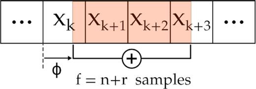
An illustration of downsampling a time series by a non-integer factor f = n + r, where n = ⌊f⌋ and 0 < r < 1.
