


ABSTRACT
It has been suggested based on analytic theory that even in non-rotating supernova progenitors stochastic spin-up by internal gravity waves (IGWs) during the late burning stages can impart enough angular momentum to the core to result in neutron star birth spin periods below |$100\, \mathrm{ms}$|, and a relatively firm upper limit of |$500\, \mathrm{ms}$| for the spin period. We here investigate this process using a 3D simulation of oxygen shell burning in a 3 M⊙ He star. Our model indicates that stochastic spin-up by IGWs is less efficient than previously thought. We find that the stochastic angular momentum flux carried by waves excited at the shell boundary is significantly smaller for a given convective luminosity and turnover time than would be expected from simple dimensional analysis. This can be explained by noting that the waves launched by overshooting convective plumes contain modes of opposite angular wavenumber with similar amplitudes, so that the net angular momentum of excited wave packets almost cancels. We find that the wave-mediated angular momentum flux from the oxygen shell follows a random walk, but again dimensional analysis overestimates the random walk amplitudes since the correlation time is only a fraction of the convective turnover time. Extrapolating our findings over the entire lifetime of the last burning stages prior to collapse, we predict that the core angular momentum from stochastic spin-up would translate into long birth spin periods of several seconds for low-mass progenitors and no less than |$100\, \mathrm{ms}$| even for high-mass progenitors.
1 INTRODUCTION
The birth spin periods of pulsars potentially provide a window into the inner workings of angular momentum transport in massive stars and of the core-collapse supernova explosion mechanism. The bulk of the observed solitary neutron star population has birth spin periods of hundreds of ms, and some as fast as tens of ms (Faucher-Giguère & Kaspi 2006; Popov et al. 2010; Popov & Turolla 2012; Gullón et al. 2014). Slow birth spin periods of several hundred ms can be inferred from age and spin-down measurements (e.g. PSR J1955+5059 in Noutsos et al. 2013), but without independent measures of the age and braking index, the slow end of the population cannot be tightly constrained. Even for young pulsars with spin periods of |$\mathord {\gt }100\, \mathrm{ms}$| (e.g. PSR J0248+6021, which has a spin period of |$217\, \mathrm{ms}$| and age |$62\, \mathrm{kyr}$|; Theureau et al. 2011), uncertainties in possible instabilities and spin-down mechanisms during the first years means that one needs to be careful in drawing conclusions from such low spin rates on the birth spin period. Despite long-standing efforts to understand the pre-collapse spin periods of massive stars (e.g. Heger, Langer & Woosley 2000; Hirschi, Meynet & Maeder 2004; Heger, Woosley & Spruit 2005) and spin-up/spin-down processes during the supernova explosion (Blondin & Mezzacappa 2007; Rantsiou et al. 2011; Wongwathanarat, Janka & Müller 2013; Kazeroni, Guilet & Foglizzo 2016; Müller et al. 2019; Stockinger et al. 2020), it is still not clear what shapes the observed period distribution.
In particular, there are still considerable uncertainties concerning the angular momentum transport processes in stellar interiors that determine the pre-collapse rotation profiles of massive stars. Stellar evolution models incorporating magnetic torques (e.g. Heger et al. 2005; Suijs et al. 2008; Cantiello et al. 2014) from the Tayler–Spruit dynamo (Spruit 2002) have long defined the state of the art for the treatment of stellar rotation in massive stars. In recent years, however, asteroseismology has revealed unexpectedly slow core rotation rates in low-mass red giants (Beck et al. 2012, 2014; Deheuvels et al. 2012, 2014; Mosser et al. 2012), which cannot be explained by the classic Tayler–Spruit dynamo, suggesting that even more efficient angular momentum transport mechanisms must operate in nature (Cantiello et al. 2014; Fuller et al. 2014; Wheeler, Kagan & Chatzopoulos 2015).
Different solutions have been proposed to resolve this problem. Fuller, Piro & Jermyn (2019) have proposed a modification of the Tayler–Spruit dynamo that efficiently slows down progenitors to be roughly consistent with both the observed neutron star birth spin periods and, unlike the Tayler–Spruit dynamo, the core rotation rates of red giants. It cannot, however, explain the rotation rates of intermediate-mass stars (den Hartogh, Eggenberger & Deheuvels 2020). As an alternative solution that does not rely on magnetic torques, many studies have investigated angular momentum transport by internal gravity waves (IGWs) in low- and high-mass stars during various evolutionary phases (e.g. Zahn, Talon & Matias 1997; Kumar, Talon & Zahn 1999; Talon & Charbonnel 2003; Charbonnel & Talon 2005; Rogers & Glatzmaier 2006; Fuller et al. 2014; Belkacem et al. 2015; Pinçon, Belkacem & Goupil 2016; Pinçon et al. 2017) and suggested that IGWs can maintain strong core–envelope coupling only up to the subgiant branch.
Angular momentum transport by IGWs could, however, again play an important role during more advanced burning stages in massive stars because the enormous convective luminosities and relatively high Mach numbers lead to a strong excitation of IGWs at convective boundaries (Fuller et al. 2015). The familiar wave filtering mechanism for prograde/retrograde modes could then effectively limit the degree of differential rotation in the interior and spin-down the core on rather short time-scales if rotation is fast to begin with (Fuller et al. 2015). The authors find that for initially rapidly rotating progenitors, angular momentum transport via g-modes is not efficient enough to explain the pulsar population. The authors find a maximum spin frequency bound from spin-down of ∼3 ms, which is consistent with the range of possible birth spins for the fastest spinning solitary pulsar (Marshall et al. 1998, spin period of 16 ms today). Additionally, Fuller et al. (2015) pointed out that IGWs could lead to a stochastic core spin-up in initially non-spinning progenitors. The idea here is that stochastically excited IGWs from the convective boundaries of the Si, O, or C shell propagate into the core, where they break and deposit their randomly varying angular momentum. The core angular momentum executes a random walk, as long as there is an influx of IGWs from strong burning shells. In principle, IGWs can also be excited by core convection or shells that end up in the core, and carry angular momentum outwards. This mirror process was found to be subdominant in the case studied by Fuller et al. (2015), however.
Rotation could potentially modify this random walk process in a non-trivial way. Once a substantial rotation rate is present in stars, the wave-filtering process (Talon & Charbonnel 2005) can change the direction of zonal mean flows, similar to the ‘quasi-biennial’ oscillations observed in the Earth’s atmosphere, where winds at the equator completely change direction (e.g. prograde to retrograde) every 14 months (Baldwin et al. 2001). Changes driven by IGWs have been studied in the context of the Sun with varying success (Kumar et al. 1999; Kim & MacGregor 2001; Talon, Kumar & Zahn 2002; Rogers & Glatzmaier 2006). These studies model the evolution of solar zonal velocity fields over year-to-decade time-scales, motivated by the observed 11-yr sunspot cycle and the solar wind’s 1.3 yr oscillation cycle. Unlike the Sun, during late burning phases the shell structure changes on time-scales of minutes, and it is unclear whether we can even expect similar long-time oscillations on secular time scales to exist. If they do, identifying them will be challenging in 3D simulations due to difficulties in identifying eigenmodes for a non-stationary background.
Fuller et al. (2015) argue that the stochastic spin-up will result in typical neutron birth periods scattering over a range about |$40\, \mathrm{ms}$| up to an effective upper limit of |$\mathord {\sim } 500\, \mathrm{ms}$| without the need to assume any progenitor rotation. If the core angular momentum is indeed determined by this stochastic spin-up process, this could explain the paucity of long spin periods of |$\mathord {\gtrsim } 500\, \mathrm{ms}$| among young neutron stars. Aside from the implications for neutron star spin periods, the excitation of IGWs during the late convective burning stages is also of interest because it could drive mass loss in supernova progenitors shortly before collapse (Quataert & Shiode 2012; Fuller 2017) or lead to envelope inflation (Mcley & Soker 2014). This could explain observations of circumstellar material (CSM) from late pre-collapse outbursts in a significant number of observed supernovae (for an overview, see Foley et al. 2011; Smith 2014,2017; Bilinski et al. 2015), although other mechanisms such as flashes from degenerate shell burning (Woosley & Heger 2015) or the pulsational pair instability (Woosley, Blinnikov & Heger 2007) may be required to account for more spectacular cases with several solar masses of CSM in Type IIn supernovae.
In this paper, we further investigate the excitation of IGWs during late-stage convective burning and its implication for stochastic core spin-up. Different from the problem of wave excitation by convection during early evolutionary stages, this problem cannot be addressed by asteroseismic measurements. The extant studies of Quataert & Shiode (2012), Fuller et al. (2015), and Fuller (2017) strongly rely on the analytic theory of wave excitation by turbulent convection that has been developed over decades (Lighthill 1952; Townsend 1966; Goldreich & Kumar 1990; Quataert & Lecoanet 2013). Numerical simulations of IGW excitation at convective boundaries have been conducted for earlier evolutionary stages in 2D (Rogers et al. 2013) and 3D (Alvan, Brun & Mathis 2014; Alvan et al. 2015; Edelmann et al. 2019), but cannot be easily extrapolated to the late, neutrino-cooled burning stages where the Péclet number is lower and compressibility effects play a bigger role. During the early evolutionary stages, asteroseismology can be used to directly test the underlying theories for IGW excitation by convection (Aerts & Rogers 2015; Aerts et al. 2017). On the other hand, a number of studies have already addressed the late burning stages in 3D (e.g. Meakin & Arnett 2007; Arnett, Meakin & Young 2008; Müller et al. 2016,2019; Cristini et al. 2017; Jones et al. 2017; Andrassy et al. 2020; Yadav et al. 2020), but without addressing the problem of stochastic spin-up.
In this study, we use a full 4|$\pi$|–3D numerical simulation to quantitatively study the idea of stochastic spin-up for the first time. We consider a 3 M⊙ He star model from Müller et al. (2019), which we evolved for 7.8 min, or |$\mathord {\sim } 35$| convective turnover times. We consider the excitation of waves by vigorous convection in the oxygen burning shell of this model to check the assumptions underlying the theory of Fuller et al. (2015, hereafter F15) for stochastic core spin-up. We focus on the outward flux of angular momentum from the oxygen shell since wave excitation at the outer boundaries of a convective shell or core is more tractable from the numerical point of view than the excitation of inward-propagating waves from the inner boundary of a convective shell. Since the physical process of wave excitation is the same, this approach none the less allows us to study the process in the relevant physical regime and check the scaling relations and dimensionless parameters used in the theory of F15.
The paper is structured as follows. In Section 2, we review key elements of the theory of F15 for the stochastic spin-up of supernova progenitor cores by IGWs. In Section 3, we describe the 3D progenitor model. In Section 4, we analyse the simulation using spherical Favre decomposition to determine the energy and angular momentum flux in convectively stable zones. We compare these results with the random walk model of F15, and finally comment on the implications of our results for neutron star birth spins. In Section 5, we discuss potential numerical issues that may affect our results, such as numerical angular momentum conservation errors, and then summarize our findings in Section 6.
2 THEORY OF STOCHASTIC SPIN-UP
Gravity waves (g-modes) are generated by turbulent convection at convective boundaries, and propagate in the neighbouring convectively stable regions. The theory of F15 relies on a few key assumptions about the wave excitation process to model the stochastic spin-up of the core in non-rotating or slowly rotating progenitors.
3 SHELL BURNING SIMULATION
The challenge is now to determine whether the key approximations in equations (1), (4), and (6) are borne out by full 3D simulations. We analyse a 3D model of convective shell burning in a non-rotating 3 M⊙ helium star from Müller et al. (2019). Following the methodology of Müller et al. (2016), we map the underlying 1D stellar evolution model from the kepler code (Weaver, Zimmerman & Woosley 1978; Heger & Woosley 2010) into the finite-volume code prometheus (Fryxell, Müller & Arnett 1989; Fryxell, Arnett & Mueller 1991) at a late pre-collapse stage about 8 min before the onset of collapse. Our simulation includes the mass shells initially located between |$2420$| and |$16\,500\, \mathrm{km}$|, which covers three distinct convective zones as illustrated (in turquoise) by the progenitor entropy profile in Fig. 1(a). Initially there are three convective burning zones: (I), (II), and (III), which are oxygen, neon, and carbon shells, respectively. The neon burning region (II) is consumed before collapse and is so thin that g-modes will in fact be able to propagate through it for much of the simulation. By |$344\, \mathrm{s}$| (5.77 min) region (II) has disappeared completely, and there is just one convectively stable region between (I) and (III), shown in Fig. 1(b). The inner boundary of the grid is contracted in accordance with the mass shell trajectory from the 1D kepler model. We use uniform spacing in log r for the radial coordinate and the axis-free overset Yin–Yang grid (Kageyama & Sato 2004) as implemented by Melson, Janka & Marek (2015) to cover the full sphere. The grid resolution is 400 × 56 × 148 zones in radius r, latitude θ, and longitude φ on each of the Yin–Yang patches, which corresponds to an angular resolution of 2°. Extremum-preserving sixth-order piecewise parabolic method (PPM) reconstruction has been implemented in prometheus following Colella & Sekora (2008).
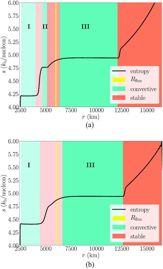
Spherically averaged profiles of the specific entropy s (solid black), against our defined regions at early (|$t=144\, \mathrm{s}$|) and late (|$t=368\, \mathrm{s}$|) times. Convective (turquoise) and convectively stable (coral) regions are labelled (I)–(III), with increasing darkness from the inner boundary to the outer boundary. Turbulent fluxes between the convective regions (I) and (III) are evaluated at the radius |$R_\mathrm{flux} =R_{m=1.65\, \mathrm{ M}_\odot }$|, which is in the convectively stable region between zones (II) and (III) up until around |$400\, \mathrm{s}$|. The second convective region disappears completely at |$344\, \mathrm{s}$|; the shell structure after the disappearance of region (II) is shown in panel (b).
4 RESULTS
4.1 Visual identification of excited modes
We run the model for 7.8 min during oxygen burning. It takes about 1 min for convection to fully develop in region (I) from the 1D initial conditions, so we only consider the phase after the first minute in our subsequent analysis.
In Fig. 2, we show 2D slices of the cube root2 of the radial velocity |$v_\mathrm{ r}^{1/3}$| and specific entropy s. We have restricted the velocity scale corresponding to |$-300 \lt v_\mathrm{ r} \lt 300\, \mathrm{km}\, \mathrm{s}^{-1}$| (|$-6.75 \lt v_\mathrm{ r}^{1/3} \lt 6.75\, \mathrm{km}^{1/3}\, \mathrm{s}^{-1/3}$|) to show both the convective motions in region (I) and the excited waves in the surrounding stable region. The boundary between region (I) enclosed by turquoise dotted lines and the stable region is clearly identifiable in the entropy plot as a relatively sharp discontinuity at a radius of about |$4400\, \mathrm{km}$|; it is evident that the convective plumes do not overshoot strongly into the stable regions. This clearly identifies the slower, laminar motions of a few |$10\, \mathrm{km}\, \mathrm{s}^{-1}$| (|$v_\mathrm{ r}^{1/3}=3.35\, \mathrm{km}^{1/3}\, \mathrm{s}^{-1/3}$|) as excited modes. We note that these wave patterns do not appear spherical, as would be expected for waves in lower Mach number flows (e.g. Horst et al. 2020), where the time-scale for convective forcing is comparable to the propagation speed. Here, |$\mathcal {M}\sim 0.1$| and the convective velocities reach a few |$100\, \mathrm{km}\, \mathrm{s}^{-1}$| (|$v_\mathrm{ r}^{1/3}=6.70$|). The excited modes are therefore of moderately high wavenumber and clearly not dominated by dipole or quadrupole modes.
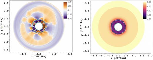
2D slices showing the cube root |$v_\mathrm{ r}^{1/3}$| of the radial velocity vr in |$\mathrm{km}\, \mathrm{s}^{-1}$| (left) and the entropy s in kb/nucleon (right) at a time of |$327\, \mathrm{s}$|, where |$v_\mathrm{ r}^{1/3} = 3.35$| and |$6.70\, \mathrm{km}^{1/3}\, \mathrm{s}^{-1/3}$| correspond to |$v_\mathrm{ r} = 40$| and |$300 \,\mathrm{km}\, \mathrm{s}^{-1}$|, respectively. In region (I) (demarcated by dotted turquoise lines), we find turbulent motions of high velocity. In the surrounding stable region outside |$r\approx 4400\, \mathrm{km}$|, we find coherent flow patterns dominated by moderately high multipoles, which is indicative of g-mode activity.
4.2 Expected IGW frequencies
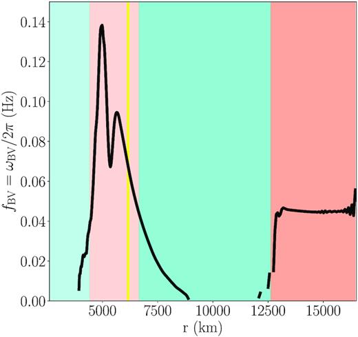
Brunt–Väisälä frequency ωBV as a function of radius r at |$368\, \mathrm{s}$| (same as Fig. 1b), after the middle convective region has disappeared. Based on this profile, gravity waves may propagate in the coral convectively stable zones at frequencies below |$\mathord {\sim } 0.1\, \mathrm{Hz}$|.
Note that, strictly speaking, the Brunt–Väisälä frequencies computed with equation (7) are only valid in the linear approximation, where the runaway (convectively unstable) or oscillation (convectively stable) of a stochastically displaced fluid parcel is determined by the local buoyancy excess upon displacement. The fact that there are real Brunt–Väisälä frequencies outside of our convectively stable regions (defined by the entropy gradient) can be explained by the deceleration of fluid parcels as they approach the boundary, where they can penetrate (overshoot) it (see Mocák et al. 2008 for a detailed explanation).
4.3 Angular momentum flux in excited waves
Strictly speaking, however, one can only properly separate the flux carried by gravity waves and acoustic waves using a decomposition of the fluctuating components into eigenmodes. When using the Favre decomposition of the energy equation, the wave energy flux is split among the three turbulent flux components. At the same time acoustic waves and entrainment contribute to the turbulent fluxes, which is particularly problematic in the case of entrainment, which produces a negative energy flux near the convective boundary.
Because of these difficulties in isolating the wave energy flux |$\dot{E}$| from region (I), we do not test equation (1), for which there is strong justification from theory and simulations anyway (Goldreich & Kumar 1990; Quataert & Lecoanet 2013; Pinçon et al. 2016). Instead, we assume |$\dot{E} = \mathcal {M} L_\mathrm{conv}$|, and directly test the dependence of |$\dot{J}$| on Lconv and |$\mathcal {M}$| in equation (4).
In Fig. 4, we plot the ratio of the turbulent angular momentum flux |$\dot{J}=4\pi r^2|\boldsymbol = \boldsymbol {F}_{\mathrm{turb}}|$| to the value |$\dot{J}_\mathrm{F15}=\tau \mathcal {M} L_\mathrm{conv}/(2\pi)$| predicted by F15. Once convection in region (I) has reached a steady state, the angular momentum flux |$\dot{J}$| only reaches a fraction of a few |$\mathord {\sim } 10^{-2}$| of the flux predicted by F15. If we accept the scaling |$\dot{E}=\mathcal {M}^{\alpha } L_\mathrm{conv}$| for the wave energy flux, this result implies that the effective average wavenumber of the excited wave packets must be much smaller than |$\bar{m}=1$| despite the fact that the excited modes have rather high angular wavenumbers as discussed in Section 4.1.4 It is, in fact, natural to expect that |$\bar{m}=1$| is not a lower bound for the average wavenumber if one considers the dynamics of wave excitation at convective boundaries. Convective plumes are driven by radial buoyancy forces and therefore hit the convective boundary almost perpendicularly. Any overshooting plume will therefore tend to launch gravity waves propagating in all directions away from the plume (i.e. with wavenumbers of opposing sign) with similar amplitude. A small asymmetry between modes of different m can still arise if the plume wanders around, but the convective updrafts and downdrafts tend to be rather stationary in simulations of convection during the neutrino-cooled burning stages, and hence there is only a small asymmetry in amplitude between excited modes of opposite m. Contrary to the assumption of F15, |$\bar{m}=1$| is therefore not a strict lower bound for a single wave packet launched by an overshooting plume; |$\bar{m}\lt 1$| is easily possible and in fact expected for waves excited by buoyancy-driven convection.
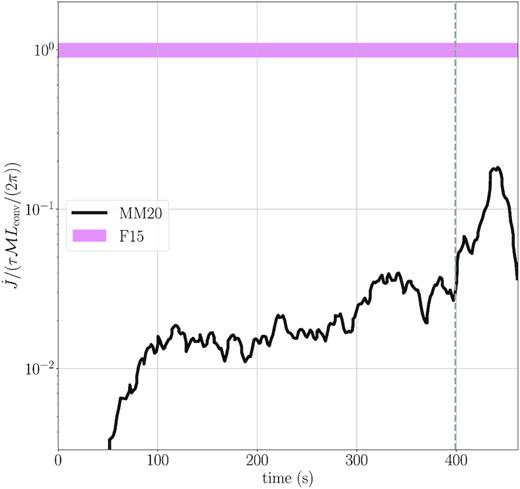
Ratio of the turbulent angular momentum flux |$\dot{J} = |\boldsymbol = \boldsymbol {F}_\mathrm{turb}|$| from our 3D simulation (MM20) to the prediction from equation (4), based on our calculations of the convective Mach number |$\mathcal {M}$| and convective burning luminosity |$\dot{Q}_\mathrm{nuc}$| (and hence the energy flux via equation 1) and convective turnover frequency. Our computed angular momentum flux is smaller by a factor of |$\mathord {\sim }10^2$| than what the model in F15 suggests when using the typical wavenumber |$\bar{m}=1$|. After around |$400\, \mathrm{s}$| (grey dashed line), the mass coordinate where we measure the angular momentum flux resides inside the inner convective region (I), so the ratio is no longer reliable.
4.4 Testing the random walk assumption
The relatively small values of the turbulent angular momentum flux already indicate that the mechanism for stochastic spin-up is considerably less efficient than F15 estimated. However, there is yet another potential problem that could further reduce the efficiency of stochastic spin-up. One might suspect that the excitation of modes by overshooting plumes is not a time-independent stochastic process that results in a random walk of the angular momentum of the convective region that launches the waves, and of the angular momentum in the destination region. Instead, there could be a regression to zero if the stochastic excitation were to predominantly produce prograde modes, which would drive the angular momentum of the driving region towards zero. Such a mechanism could operate independently of the familiar filtering mechanism for prograde and retrograde modes and limit stochastic fluctuations of the angular momentum of convective shells even when there is no strong differential rotation.
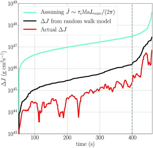
The change in angular momentum, ΔJ, inside the mass coordinate m = 1.65 M⊙ based on the three different formulations of ΔJ in equations (19)–(21). The angular momentum computed from the simulation (equation 20) is in red, and the angular momentum computed assuming a random walk via equation (19) is in black. The angular momentum calculated from equation (21) assuming the relation (4) between the angular momentum flux and the convective luminosity is in cyan. After |$400\, \mathrm{s}$| (dashed grey line) the mass coordinate where we measure the flux lies inside the convective region (I) (see Fig. 1). The significant growth of ΔJ in the last |$70\, \mathrm{s}$| is the result of stochastic angular momentum redistribution inside the convective zone, and not associated with a flux of IGWs. The wave packet random walk model is no longer applicable during this phase and cannot be used to infer spin-up of the region from IGWs.
Interestingly, even though ΔJRW (black) still overpredicts the actual time-integrated angular momentum flux ΔJ (red) by a factor of 5 on average, this is not a huge discrepancy. The growth of ΔJ appears roughly compatible with a random walk, only with an effective correlation time that is |$4{{\ \rm per\ cent}}$| of what is assumed in F15, since the spin-up scales with the square root of the correlation time, |$\Delta J_\mathrm{RW}\propto \sqrt{\tau }$|. This short correlation time may be related to the rather high wavenumbers of the excited modes. The effective correlation time of the random walk must reflect the characteristic time-scale of the forcing motions with similar wavenumbers, or in other words, of relatively small-scale structures in the convective flow, which evolve on significantly shorter time-scales than τconv.
In comparing to F15, one needs to bear in mind one important caveat on our simulation set-up. What critically matters in the model of F15 is the angular momentum flux into the convectively stable core, while we measure the flux between two convective regions. Unlike inside the core, where waves will damp and break, outward-propagating waves here are subject to reflection at the next convective boundary, and it is possible that undamped waves produce standing waves, which potentially destructively interfere, resulting in a smaller angular momentum flux than the single-mode wave packet would predict. It is therefore possible that the discrepancy with F15 is due in part to an (incomplete) cancellation of the angular momentum flux by reflected waves, rather than to a shorter correlation time. However, if the true correlation time of the forcing motions were of the order of the convective turnover time τconv, one would still expect that at least the direction of the angular momentum carried by waves should be stable on this longer time-scale. To check this, we compute the correlation time for the direction of the vector |$\dot{J}$|; a correlation time closer to the convective turnover time of |$\mathord {\sim }13\, \mathrm{s}$| would indicate that we are measuring flux from interfering reflected waves. The correlation time of the direction of |$\dot{J}$| is only |$0.5 \, \mathrm{s}$|, consistent with our inferred correlation time of the random walk. However, it remains difficult to distinguish standing and travelling waves in Fig. 2, and we cannot rule out some contamination of wave reflection as a contributor to the low angular momentum. Ultimately, simulations of IGW excitation at the inner convective boundaries will still be required to completely exclude contributions from wave reflection.
Regardless of these potential complications, it is important to stress that our simulation actually supports the assumption that stochastic wave excitation will lead to the core angular momentum executing a random walk, albeit with a shorter correlation time. However, because the assumption of |$\bar{m}=1$| is not valid and because the correlation time of the random walk is somewhat shorter than the convective turnover time in our simulations, the original model of F15 overpredicts ΔJ by several orders of magnitude.
On the other hand, Fig. 5 suggests that the late convective burning stages might stochastically affect the remnant angular momentum in a different manner. During the last |$70\, \mathrm{s}$| of the simulation, the analysis radius lies inside the oxygen shell, and the measured ΔJ indicates stochastic internal redistribution of angular momentum within the shell. This stochastic redistribution of angular momentum could potentially spin-up the inner regions of the shell considerably. In the present example, the time-integrated flux of angular momentum ΔJ within the oxygen shell during the last |$70\, \mathrm{s}$| is 10 times bigger than the time-integrated wave-mediated flux of angular momentum out of the oxygen shell. If only part of the oxygen shell is ejected during the supernova explosion, the total angular momentum within the ‘mass cut’ may be considerable. If the mass cut were placed at 1.65 M⊙ (which is much larger than is realistic for this model; Müller et al. 2019), the resulting neutron star spin period would be of order |$100\, \mathrm{ms}$|. Naturally, the theory of stochastic IGW excitation cannot be applied to stochastic variations within convective regions close to the mass cut, so one cannot make generic predictions about the importance of this phenomenon. However, 3D supernova progenitor models that include this effect naturally anyway are becoming more widely used.
4.5 Estimate of neutron star spin periods
Fig. 5 shows that during the simulation time of about 7 min, the angular momentum transported out of the oxygen shell from the outer boundary is about |$2\times 10^{45}\, \mathrm{g}\, \mathrm{cm}^2\, \mathrm{s}^{-1}$|. If a similar amount of angular momentum is transported inwards into the core, and the angular momentum is conserved during the collapse to a neutron star, this would result in a neutron star rotation rate |$\omega \approx 1\, \mathrm{rad}\, \mathrm{s}^{-1}$| of a typical neutron star moment of inertia |$\mathord {\sim }1.5 \times 10^{45}\, \mathrm{g}\, \mathrm{cm}^2$|. However, our simulation only covers the last phase in the life of the second oxygen shell. To gauge the actual impact of stochastic spin-up, we need to extrapolate our results to the entire lifetime of a shell similar to F15, but with different efficiency factors.
5 EFFECTS OF NUMERICAL CONSERVATION ERRORS
Finite-volume methods as used in prometheus generally cannot conserve total angular momentum to machine accuracy (unlike smoothed particle hydrodynamics). Moreover, angular momentum transport in any grid-based or particle-based simulation will be affected to some degree by numerical dissipation. One may justifiably ask whether non-conservation of total angular momentum or numerical dissipation has any bearing on our simulation of stochastic spin-up. In the context of the preceding discussion, it is especially pertinent, whether the convective region (I) is indeed spun up in the opposite direction to the angular momentum that is lost by waves. This specific problem can already be addressed here, though more extensive resolution studies and simulations with different reconstruction and discretization schemes naturally remain desirable for the future.
In Fig. 6, we compare the left-hand side and the right-hand side of equation (27) for the x-, y-, and z-component of the angular momentum. For all three components, at the end of the simulation the direction of the convective shell angular momentum is indeed the opposite sign of the angular momentum leaving at the flux boundary. Early on, the evolution of |$\boldsymbol = \boldsymbol {J}$| is dominated by numerical errors, the y-component in particular shows a significant drift over the first |$200\, \mathrm{s}$|. As soon as convection is fully developed and the excited waves from the convective boundary carry a significant angular momentum flux, the evolution of the total angular momentum in the analysis region clearly follows the time-integrated angular momentum flux. This suggests that angular momentum conservation errors do not significantly affect our analysis at times later than |$\mathord {\sim } 200\, \mathrm{s}$|. Of course, more subtle numerical issues, such artificial damping of the excited waves, may limit the accuracy of our results and need to be further investigated in the future. However, we believe that the key findings of this study will likely remain robust. The code clearly has the ability to evolve relatively weak waves, and the waves that would need to be resolved for the mechanism of F15 to work effectively are not of extremely short wavelength, so that excessive dissipation is likely not a critical problem.
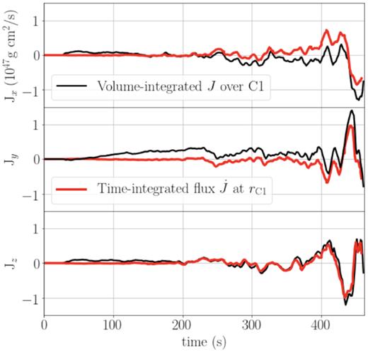
Time-integrated angular momentum flux at the fixed boundary C1 (red) and the (negative) integrated angular momentum over the volume enclosed by C1 (black) in the x, y, and z directions. For each component, the angular momentum in the spun-up convective shell volume is consistent with the angular momentum flux leaving the volume.
6 CONCLUSIONS
Using the 3D hydrodynamics code prometheus, we studied the angular momentum flux from stochastically excited IGWs during oxygen shell burning in an initially non-rotating massive star. Our findings allow us to better assess the efficiency of stochastic wave excitation as a process for core spin-up, which has been suggested by F15 based on analytic theory.
In agreement with the theory of F15, we find that the IGW-mediated flux of angular momentum out of a convective shell in a non- or slowly rotating progenitor can indeed be described by a random walk process. However, we find that the correlation time of this random walk process is only a fraction of the convective turnover time and hence significantly shorter than assumed by F15. This reduces the amplitude of the random walk by a factor of several.
We also find a smaller ratio between the angular momentum flux carried by the excited IGWs and the convective luminosity by more than an order of magnitude than assumed by F15. We ascribe this discrepancy to the fact that the assumption of an average zonal wavenumber |$\bar{m}=1$| of individual IGW ‘wave packets’ is too optimistic, since IGWs excited by overshooting convective plumes will generally contain modes with opposite zonal wavenumber m of almost equal amplitude. Therefore the average zonal wavenumber |$\bar{m}$| of each wave packet will be much smaller than unity and the net angular momentum carried by the wave packet will be very small.
The combination of a shorter effective correlation time and a smaller instantaneous angular momentum flux results in a time-integrated stochastic angular momentum flux from the oxygen shell that is about a factor of |$\mathord {\sim }10^2$| smaller than predicted by the model of F15. It should be pointed out, however, that our simulation is compatible with their analytic scaling laws; it merely suggests that the relevant dimensionless parameters of the model may be quite small.
The characteristic spin period from stochastic spin-up of the core by IGWs over the entire life of a convective burning shell can be estimated based on the mass, radius, width, and lifetime of the shell from 1D stellar evolution models using a simple scaling relation (equation 26). Extrapolating our simulation results over the entire lifetime of convective shells, we estimate that stochastic spin-up by IGWs alone would result in neutron star birth spin periods of several seconds for low-mass stars and down to |$\mathord {\sim }0.1\, \mathrm{s}$| for high-mass stars with thick oxygen shells. These spin rates are slower than predicted by F15 by one to two orders of magnitude. Thus our findings suggest that stochastic spin-up of progenitor cores will usually not play a major role in determining the core spin rates of massive stars and neutron star birth periods, because stochastic spin-up processes during the supernova explosion will impart more angular momentum on to the neutron star.
It remains to be seen, however, to what extent the efficiency factors for IGW excitation and stochastic core spin-up found in our simulation depend on the detailed properties of convective zones and the structure of the convective boundary. For example, the correlation time of the random walk and the average zonal wavenumber will depend on the typical size of the convective eddies. Convection zones with pronounced large-scale flow patterns and fewer but stronger plume impact events may provide more favourable conditions for stochastic core spin-up. In future, one should also investigate stiffer convective boundaries with sharp entropy jumps. The inner convective boundaries, which are of highest relevance for the problem of stochastic spin-up, are considerably stiffer than the convective boundary considered in this study. Simulating IGW excitation at inner convective boundaries would also be desirable to exclude any potential artefacts from wave reflection at shell boundaries further outside. Moreover, the dependence of stochastic spin-up on the convective Mach number should be investigated numerically to confirm the predicted scaling laws. We also note that stochastic angular momentum redistribution within convective zones close to the mass cut could be relevant for predicting neutron star birth spin periods. This effect is already implicitly included in modern 3D supernova progenitor models. Better understanding convection, wave excitation, and angular momentum transport by 3D simulations will remain challenging because of the technical difficulties of low Mach number flow, stringent resolution requirements at stiff convective boundaries, and the numerical problem of angular momentum conservation. However, 3D simulations of convective burning are clearly proving useful in understanding angular momentum transport processes in supernova progenitors.
ACKNOWLEDGEMENTS
We acknowledge fruitful discussions with A. Heger and I. Mandel. We thank J. Fuller, D. Lecoanet, and the anonymous referee for helpful suggestions and comments on an earlier version that improved this paper. LOM acknowledges support by an Australian Government Research Training (RTP) Scholarship. BM has been supported by the Australian Research Council through Future Fellowship FT160100035 and partly as an Associate Investigator of the ARC Centre of Excellence OzGrav (CE170100004). This research was undertaken with the assistance of resources from the National Computational Infrastructure (NCI), which is supported by the Australian Government and was supported by resources provided by the Pawsey Supercomputing Centre with funding from the Australian Government and the Government of Western Australia.
DATA AVAILABILITY
The data underlying this paper will be shared on reasonable request to the authors, subject to considerations of intellectual property law.
Footnotes
Properly speaking, each component ΔJi will execute an independent random by with step size |$\delta J_i=\delta J/ \sqrt{3}$| if the angular momentum of the wave packets is randomly oriented, but the factor |$1/\sqrt{3}$| cancels again when we consider the expectation value of ΔJ2 since 〈ΔJ2〉 = 3〈ΔJ2〉.
We plot the cube root to better identify flow features with small velocities.
One could also define Lconv as the maximum of the turbulent energy flux |$\dot{E}$| inside a convective region. This yields similar, but more noisy results.
Alternatively, one might surmise that the excited modes have frequencies higher than ω = 2|$\pi$|/τ, but unless there is resonant excitation it is unavoidable that the frequency spectrum of the excited modes roughly reflects the frequency spectrum of the turbulent driving motions.
