


ABSTRACT
Historically, photometry has been largely used to identify stellar populations [multiple populations (MPs)] in globular clusters (GCs) by using diagrams that are based on colours and magnitudes that are mostly sensitive to stars with different metallicities or different abundances of helium, carbon, nitrogen, and oxygen. In particular, the pseudo-two-colour diagram called chromosome map (ChM), allowed the identification and the characterization of MPs in about 70 GCs by using appropriate filters of the Hubble Space Telescope (HST) that are sensitive to the stellar content of He, C, N, O, and Fe.
We use here high precision HST photometry from F275W, F280N, F343N, F373N, and F814W images of ω Centauri to investigate its MPs. We introduce a new ChM whose abscissa and ordinate are mostly sensitive to stellar populations with different magnesium and nitrogen, respectively, in monometallic GCs. This ChM is effective in disentangling the MPs based on their Mg chemical abundances, allowing us to explore, for the first time, possible relations between the production of these elemental species for large samples of stars in GCs.
By comparing the colours of the distinct stellar populations with the colours obtained from appropriate synthetic spectra we provide ‘photometric-like’ estimates of the chemical composition of each population. Our results show that, in addition to first-generation (1G) stars, the metal-poor population of ω Cen hosts four groups of second-generation stars with different [N/Fe], namely, 2GA–D. 2GA stars share nearly the same [Mg/Fe] as the 1G, whereas 2GB, 2GC, and 2GD are Mg depleted by ∼0.15, ∼0.25, and ∼0.45 dex, respectively. We provide evidence that the metal-intermediate populations host stars with depleted [Mg/Fe].
1 INTRODUCTION
The colour−magnitude diagrams (CMDs) of most Galactic and extragalactic globular clusters (GCs) are composed of distinct photometric sequences that are detected among stars at different evolutionary stages and correspond to stellar populations with different content of helium and light elements (Milone et al. 2012b, 2020, and references therein). Specifically, most GCs host a first generation (1G) of stars that share the same chemical composition as field stars with similar metallicities and second stellar generations (2G) that are enhanced in helium nitrogen and sodium and depleted in carbon and oxygen (e.g. Kraft et al. 1993; Gratton, Carretta & Bragaglia 2012; Bastian & Lardo 2018; Milone et al. 2018; Marino et al. 2019, and references therein).
The star-to-star variation of light elements and the corresponding correlations and anticorrelations observed in GCs (e.g. Hesser, Hartwick & McClure 1977; Kraft et al. 1993; Ivans et al. 2001; Marino et al. 2008; Carretta et al. 2009; Mészáros et al. 2015) is understood as the results of CNO cycling and p-capture processes at high temperatures. These processes include the Mg–Al chain, effective at temperatures higher than ∼7 × 10⁷ K, which produces Al at the expenses of Mg and is responsible for the Mg–Al anticorrelations observed in some GCs from spectroscopy (e.g. Carretta 2015; Masseron et al. 2019). Indeed, Mg abundances are proxies of stellar nucleosynthesis processes occurring at higher temperature than those responsible for the classic, and much more widespread, N–C/Na–O anticorrelations.
In addition to internal variations of light elements, some GCs exhibit stellar populations with different content of heavy elements, including iron and s-process elements (e.g. Da Costa et al. 2009; Marino et al. 2009, 2015; Carretta et al. 2010; Yong et al. 2014; Johnson et al. 2017).
Clusters with heavy element variations are called Type II GCs and comprise ∼17 per cent of the total number of Galactic GCs (Milone et al. 2017a, 2020). A common feature of Type-II GCs is that stars with similar metallicities host stellar populations with different light-elements abundances (e.g. Marino et al. 2009, 2011b; Milone et al. 2015, 2017a).
The origin of MPs is one of the most-debated open issues of stellar astrophysics, which could have significantly affected the assembly of the Galactic halo and possibly the reionization of the Universe (e.g. Renzini et al. 2015; Renzini 2017).
According to some scenarios, GCs have experienced multiple star formation episodes and 2G stars formed out of the material ejected by more-massive 1G stars (e.g. Ventura et al. 2001; Decressin et al. 2007; D’Ercole et al. 2008; Denissenkov & Hartwick 2014; D’Antona et al. 2016; Calura et al. 2019). Alternatively, GC stars are coeval and exotic phenomena that occurred in the unique environment of the proto GCs are responsible for the chemical composition of 2G stars (e.g. Bastian et al. 2013; Gieles et al. 2018). We refer to Renzini et al. (2015) for critical discussion on the various scenarios.
Various photometric diagrams have been exploited in the past decade to disentangle multiple populations (MPs) in GCs and allowed to identify and characterize MPs in more than seventy Galactic and extragalactic clusters (e.g. Milone et al. 2017a). Most of these diagrams are based on U-band photometry, which allows to distinguish 1G from 2G stars mainly through the effect of NH molecules on the ultraviolet stellar flux (e.g. Marino et al. 2008; Yong et al. 2008; Milone et al. 2012a, 2015).
Some work is based on CMDs made with a wide colour baseline, which is sensitive to stellar populations with different helium abundances. Indeed, main-sequence (MS) and red giant branch (RGB) stars enhanced in helium are hotter, hence bluer than stars with the same luminosity and primordial helium (Y ∼ 0.25) (e.g. D’Antona et al. 2002; Bedin et al. 2004; Piotto et al. 2007; Milone et al. 2018). Similarly, the U − V or U − I colours are widely used to distinguish stellar populations with different total metal content (Z, e.g. Marino et al. 2015; Milone et al. 2017a).
Milone et al. (2015) introduced a new photometric diagram called chromosome map (ChM) to identify and characterize the distinct stellar populations of GCs. The ChM is a pseudo-two-colour diagram of MS, RGB, or asymptotic-giant branch (AGB) stars, where the photometric sequences are verticalized in both dimensions. It maximizes the separation between stellar populations with different He, C, N, O, and Fe.
Near infrared (NIR) photometry is a powerful tool to identify MPs of M-dwarfs with different oxygen abundances and the F110W and F160W filters of the WFC3/NIR camera on board of HST are the most widely used filters (e.g. Milone et al. 2012b, 2019). Indeed, the F160W band is heavily affected by absorption from various molecules involving oxygen, including H2O, while F110W photometry is almost unaffected by the oxygen abundance. As a consequence, second-generation (2G) stars, which are depleted in O with respect to the 1G, have brighter F160W magnitudes and redder F110W−F160W colours than the 1G.
In summary, all photometric diagrams used to detect multiple populations are based on colours and magnitudes that are mostly sensitive to the abundances of helium, nitrogen, oxygen, and metallicity of stars in the distinct populations.
While photometry has been successful in identifying stellar populations with different C/N/O/Na in GCs, to date, it was almost blind to stars that are composed of material exposed to higher temperature H burning, e.g. depleted in Mg with respect to the 1G. In this paper, we introduce new photometric diagrams to disentangle stars based on their magnesium abundances. This is the first time that multiple populations with different [Mg/Fe] are identified from photometry alone.
Our target, ω Centauri is the GC where multiple populations have been first detected (Woolley 1966) and one of the most-studied clusters in the context of MPs (e.g. Anderson 1997; Lee et al. 1999; Pancino et al. 2000; Bedin et al. 2004; Ferraro et al. 2004; Sollima et al. 2005, 2007; Bellini et al. 2010).
ω Centauri is an extreme Type II GC, which hosts at least 16 populations that span a wide interval of metallicity, (from [Fe/H] ≲ −2.0 to [Fe/H]∼−0.6) (e.g. Freeman & Rodgers 1975; Norris & Da Costa 1995; Norris, Freeman & Mighell 1996; Suntzeff & Kraft 1996; Johnson & Pilachowski 2010; Marino et al. 2011b), reach extreme abundances of helium and light elements (e.g. Norris 2004; Tailo et al. 2016; Bellini et al. 2017; Milone et al. 2017b), and exhibit star-to-star magnesium variations (Gratton 1982; Norris & Da Costa 1995; Da Costa, Norris & Yong 2013; Mészáros et al. 2020). In particular, similarly to what is observed in other Type-II GCs, stellar populations of ω Centauri with any given metallicity span a wide range in light-elements abundances (e.g. Johnson & Pilachowski 2010; Marino et al. 2010, 2011a, 2012; Gratton et al. 2011).
The paper is organized as follows. Section 2 describes the data set and the data reduction to derive the photometric diagrams presented in Section 3. The theoretical ChMs and the photometric diagrams from isochrones are discussed in Section 4, while Sections 5 and 6 are focused on the metal-poor and metal-rich stellar populations of ω Cen, respectively. Summary and conclusions are provided in Section 7.
2 DATA AND DATA ANALYSIS
The main data set used in this work is composed of images collected through the F275W, F280N, F343N, F373N, and F814W filters of the Ultraviolet and Visual Channel of the Wide Field Camera 3 (UVIS/WFC3) on board of Hubble Space Telescope (HST). The main properties of these images are summarized in Table 1. Photometry and astrometry have been performed from images corrected from the poor charge transfer efficiency (see Anderson & Bedin 2010). We used the computer program KS2, that is the evolution of |$kitchen\_sink$|, originally written to reduce two-filter images collected with the Wide-Field Channel of the Advanced Camera for Survey of HST (Anderson et al. 2008). As discussed by Sabbi et al. (2016) and Bellini et al. (2017), KS2 adopt two different methods to derive high-precision measurements of stars with different luminosities. To determine magnitudes and positions of faint stars we combine information from all exposures and determine the average stellar positions. Once the positions of faint stars are fixed we fit each exposure pixel with the appropriate effective point spread function (PSF) solving for the flux only. Bright stars are measured in each individual exposure by fitting the best-PSF model and the resulting magnitudes and positions are then averaged.
Description of the HST images used in the paper.
| FILTER | DATE | N×EXPTIME | PROGRAM | PI |
|---|---|---|---|---|
| F275W | Jul 15 2009 | 35 + 9 × 350 s | 11452 | J. Kim Quijano |
| F275W | Jan 12 – Jul 4 2010 | 22 × 800 s | 11911 | E. Sabbi |
| F275W | Feb 2 2011 | 9 × 800 s | 12339 | E. Sabbi |
| F280N | Feb 26 2015 | 600 s | 14031 | V. Kozhurina-Platais |
| F280N | Feb 1 2016 | 2 × 800 + 4 × 850 s | 14393 | V. Kozhurina-Platais |
| F343N | Feb 26 2015 | 600s | 14031 | V. Kozhurina-Platais |
| F343N | Mar 3 2016 | 5 × 510 + 4 × 545 s | 14393 | V. Kozhurina-Platais |
| F373N | Feb 26 2015 | 450 s | 14031 | V. Kozhurina-Platais |
| F373N | Mar 25 2016 | 5 × 500 s | 14393 | V. Kozhurina-Platais |
| F814W | Jul 15 2009 | 35 s | 11452 | J. Kim Quijano |
| F814W | Jan 10–Jul 04 2010 | 27 × 40 s | 11911 | E. Sabbi |
| F814W | Feb 15–Mar 24 2011 | 9 × 40 s | 12339 | E. Sabbi |
Instrumental magnitudes are calibrated into the Vega-mag system by using the updated photometric zero-points1 and following the recipe by Bedin et al. (2005). Stellar positions are corrected for geometrical distortion by using the solutions provided by Bellini & Bedin (2009) and Bellini, Anderson & Bedin (2011). Finally, photometry was corrected for differential reddening as in Milone et al. (2012b).
To increase the number of filters and better constrain the abundances of helium, carbon, nitrogen, oxygen, and magnesium of the stellar populations of ω Cen, we used the photometric and astrometric catalogues from Milone et al. (2017a, 2018), which include photometry obtained from images collected through 31 filters of UVIS/WFC3. Details of the data set and the data reduction are provided by Milone et al. (2017a, 2018). In summary, our data base comprises photometry in 36 bands: F218W, F225W, F275W, F280N, F300X, F336W, F343N, F373N, F390M, F373N, F390M, F390W, F395N, F410M, F438W, F467M, F469N, F475W, F487N, F502N, F555W, F606W, F621M, F625W, F631M, F645M, F656N, F657N, F658N, F673N, F673N, F680N, F689M, F763M, F680N, F689M, F763M, F775W, F814W, F845M, and F953N.
3 PHOTOMETRIC DIAGRAMS
In this section, we construct the photometric diagrams that will be exploited to analyse stellar populations with different Mg in ω Cen, starting from of the spectral features most sensitive to this element. Based on synthetic spectra of RGB stars with different chemical composition, Milone et al. (2018) show that [Mg/Fe] variations have a negligible effect on magnitudes in optical bands but provide significant flux variations in ultraviolet bands (see also Sbordone et al. 2011).
As an example, in the upper panel of Fig. 1 we compare the spectra of two RGB stars that have the same chemical abundances in all the elements, except for C, N, O, and Mg, as quoted in the figure. Specifically, the red spectrum is indicative of a 1G stars, whereas the blue spectrum corresponds to the 2G. We calculated the ratio between the fluxes (f1 and f2) of the blue and red spectra and plotted in the middle panel of Fig. 1 the quantity −2.5log f1/f2 against λ. Lower panels show the transmission curves of the F275W, F280N, F343N, and F373N filters of WFC3/UVIS.
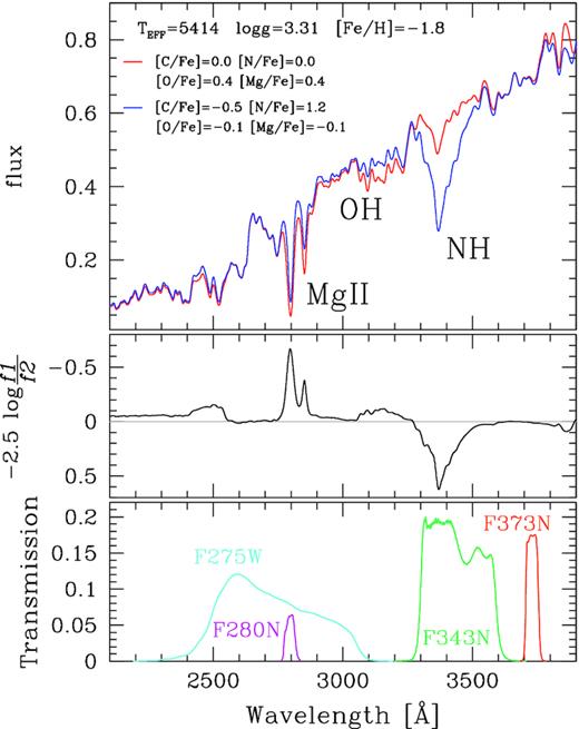
Comparison of two synthetic spectra with the same stellar parameters and metallicity quoted in the inset but different abundances of light elements (top panel). The main spectral features that are responsible for the differences between the fluxes of the two spectra are also indicated. In the middle panel, we plot the quantity −2.5log f1/f2 as a function of the wavelength, where f1 and f2 are the fluxes of the red and the blue spectrum, respectively. Lower panel shows the transmission curves of the F275W, F280N, F343N, and F373N WFC3/UVIS filters.
Clearly, the F280N band, which includes the strong Mg-II lines at λ ∼ 2800 Å is the most efficient filter on board of HST to identify stars with different values of [Mg/Fe]. The Mg-rich star is about 0.25 mag fainter in F280N than the Mg-poor one, the flux difference drops to ∼0.02 in F275W. Hence, mF275W − mF280N is an efficient colour to identify stellar populations with different magnesium abundances.
Moreover, Fig. 1 reveals that the mF343N − mF373N colour is sensitive to stellar populations with different nitrogen abundances. Indeed, the F343N filter includes the NH molecular bands around λ ∼ 3370 Å, whereas the spectral region covered by the F373N filter is poorly affected by light-element variations.
Since mF275W − mF280N and mF343N − mF373N are short colour baselines, they are both poorly sensitive to temperature and reddening differences among stars with similar luminosities.
The observed mF814W versus mF275W − mF280N CMD of ω Cen is shown in the upper-left panel of Fig. 2. The RGB exhibits two main parallel sequences in the F814W magnitude interval between ∼16.5 and ∼13.8, as highlighted in the Hess-diagram plotted in the upper-right panel. The two RGB components seem to merge together at mF814W ≲ 13.8. Additional RGB stars exhibit redder mF275W − mF280N colours than the bulk of ω Cen RGB stars. Their colour distance from the main RGB increases when we move from the base of the RGB towards the RGB tip.
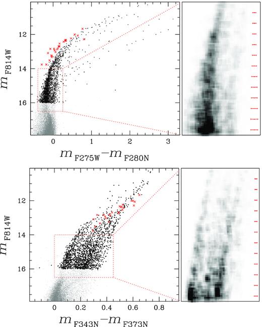
Comparison between the mF814W versus mF275W − mF280N CMD of ω Cen (top), which is very sensitive to stellar populations with different magnesium content, and the mF814W versus mF343N − mF373N CMD (bottom), which highlights stars with different nitrogen abundance. RGB stars brighter than mF814W = 16.5 are marked with black dots, while red crosses indicate AGB stars. Right-hand panels show the Hess diagrams for stars in the rectangular regions shown in the right-hand panels.
The lower panels of Fig. 2 show the mF814W versus mF343N − mF373N CMD for ω Cen RGB stars (left) and the corresponding Hess diagram for RGB stars with 14.0 < mF814W < 16.5. RGB stars of ω Cen span a wide range of mF343N − mF373N and exhibit four main stellar overdensities that indicate stellar populations with different nitrogen content.
For completeness, we mark with red crosses the asymptotic giant branch stars selected from the mF814W versus mF606W − mF814W CMD. Since AGB stars have comparable stellar parameters as RGB stars, a variation in light elements would produce similar broadening in the AGB sequences. The fact that the AGB is narrower than the RGB in both CMDs of Fig. 2 suggests that stellar populations with extreme contents of nitrogen and magnesium avoid the AGB phase, in close analogy with what is observed in other GCs (e.g. NGC 6752, NGC 2808, and NGC 6266; Campbell et al. 2013; Lapenna et al. 2015; Wang et al. 2016; Marino et al. 2017).
4 COMPARISON WITH SIMULATED MULTIPLE POPULATIONS
As discussed in the Section 1, ω Cen exhibits large star-to-star metallicity variations, and the stellar populations with different [Fe/H] host sub stellar populations with distinct content of helium and light element abundance. To investigate the physical reasons that are responsible for the multiple RGBs shown in Fig. 2, we first compare in Section 4.1 isochrones from the Dartmouth data base (Dotter et al. 2008) with different metallicities and helium contents. Then, in Section 4.2, we investigate the effect of light-element abundance variations on the CMDs by using mono-metallic isochrones with different content of He, C, N, O and Mg.
4.1 Stellar populations with different metallicities
Fig. 3 shows the MF814W versus MF275W − MF280N (left-hand panel) and the MF814W versus MF343N − MF373N (right-hand panel) CMDs for isochrones from Dotter et al. (2008) with different iron and helium abundances. Specifically, we considered isochrones with [Fe/H] = −1.8 and [Fe/H] = −1.5, which correspond to the two main peaks in the metallicity distribution based on high-resolution spectroscopy (Marino et al. 2011b), that are represented with blue and green colours, respectively. Moreover, we used isochrones with [Fe/H]=−1.0 and [Fe/H]=−0.6, which are representative to the most metal-rich stellar populations of ω Cen. The isochrones represented with continuous lines have helium abundance Y = 0.25 + 1.5 Z, where Z is the total metal abundance, while those isochrones plotted with dotted lines have helium Y = 0.40.
![Dartmouth isochrones (Dotter et al. 2008) in the MF814W versus MF275W − MF280N (left-hand panel) and MF814W versus MF343N − MF373N (right-hand panel) planes for 13-Gyr old stellar populations with [α/Fe] = 0.4 and with the abundances of iron and helium listed in the inset of left-hand panel. The RGB sequences comprise the isochrone segments brighter than MF814W ∼ 3.0.](https://oup.silverchair-cdn.com/oup/backfile/Content_public/Journal/mnras/497/3/10.1093_mnras_staa2119/1/m_staa2119fig3.jpeg?Expires=1750414428&Signature=fbQEYW64BhAtsGzwOc8K-HkcuunOs~~mEEZJ3yaFbsLTUyytrVt6sEX~qlY-FjW7afj7ZbXifUskVrzvwRp1VgzsfgT0OA2z1iG3SyAAA1I7IvB8aoLsGntle7jN2fw6epGBgOJQya34mrPSh53yNeCEdvb2L6bCWwzISKI39psO~aJuTz7hMk~4zc3-L6y1C-ZRo0GpnUIvmsAoZOqPSRa6D9hvAiA5kUO15t17bpZeiymk0qiTg8MNcBu8CjUoG0qLAzfTGFCvkCigxbtqrx2oZFOehihb0PgEamWlNkdF0ct8LvHrvt~y0~FB0GyMKb47zvntNi9QQa4lzOQ-Ng__&Key-Pair-Id=APKAIE5G5CRDK6RD3PGA)
Dartmouth isochrones (Dotter et al. 2008) in the MF814W versus MF275W − MF280N (left-hand panel) and MF814W versus MF343N − MF373N (right-hand panel) planes for 13-Gyr old stellar populations with [α/Fe] = 0.4 and with the abundances of iron and helium listed in the inset of left-hand panel. The RGB sequences comprise the isochrone segments brighter than MF814W ∼ 3.0.
A significant separation along the RGB is apparent at very high metallicity and in the upper portion of the RGB with the metal-rich isochrones characterized by redder MF275W − MF280N colours than metal-poor ones. The magnitude where the metal-rich isochrones cross the metal-poor ones depends on the value of [Fe/H]. As an example, the isochrones with [Fe/H] = −1.5, [Fe/H] = −1.0, and [Fe/H] = −0.6 intersect the [Fe/H] = −1.8 isochrone at MF814W ∼ 0.0, ∼0.5, and ∼2.7, respectively. An exception is provided by the isochrone with [Fe/H] = −0.6, which is redder than the used metal-poor isochrones along the entire RGB. Helium-rich isochrones have almost the same MF275W − MF280N colour as the metal-poor ones and become redder at brighter luminosities.
The right-hand panel of Fig. 3 shows that the low RGBs of the analysed metal-rich isochrones typically have redder MF343N − MF373N colours than those of metal-poor ones. The most metal rich isochrone, which is bluer than isochrones with [Fe/H] = −1.5 and [Fe/H] = −1.0, is a remarkable exception. The isochrones with different [Fe/H] cross each other and change their relative MF343N − MF373N colours in the upper part of the RGB. Helium-rich RGB stars of the isochrones with [Fe/H] ≥ −1.5 are redder than stars with Y∼ 0.25 and the same F814W magnitude, while the RGBs of the two isochrones with [Fe/H] = −1.8 and different helium abundances are nearly coincident for MF814W ≳ −1.5.
4.2 Stellar populations with different light-element abundances
To investigate how the abundances of C, N, O, Mg affect the position of stars in the CMDs of mono-metallic GCs, we derived the colours and magnitudes of isochrones with different abundances of carbon, nitrogen, oxygen, and magnesium by using model atmospheres and synthetic spectra, in close analogy with what done in previous papers from our team (e.g. Milone et al. 2012a, 2018). In a nutshell, we extracted 15 points along the isochrones and extracted their effective temperatures, Teff, and gravities, log g. For each pair of stellar parameters we calculated a reference spectrum with the chemical composition of 1G stars and a comparison spectrum, with the content of C, N, O, and Mg of 2G stars. Specifically, we assumed for 1G stars Y = 0.246, solar-scaled abundances of carbon and nitrogen, [O/Fe] = 0.4, and [Mg/Fe] = 0.4.
We constructed model atmosphere structures by using the computer program ATLAS12 developed by Robert Kurucz (Kurucz 1970, 1993; Sbordone et al. 2004), which exploits the opacity-sampling technique and assumes local thermodynamic equilibrium. We assumed a microturbulent velocity of 2 km s−1 for all models. Synthetic spectra are computed over the wavelength interval between 1000 and 12 000 Å with SYNTHE (Kurucz & Avrett 1981; Castelli 2005; Kurucz 2005; Sbordone, Bonifacio & Castelli 2007) and have been integrated over the bandpasses of the ACS/WFC and UVIS/WFC3 filters used in this paper to derive the corresponding magnitudes. We calculated the magnitude difference, δmX, between the comparison and the reference spectrum. The magnitudes of the 2G isochrones are derived by adding to the 1G isochrones the corresponding values of δmX.
We plot in Fig. 4 five isochrones with the same iron abundance, [Fe/H] = −1.7, but different content of He, C, N, O, and Mg in the MF814W versus MF275W − MF280N and MF814W versus MF343N − MF373N planes. The specific chemical composition of each isochrone is quoted in Table 2 and corresponds to constant [(C+N+O)/Fe]. In particular, we assumed that the green and the red isochrones have [Mg/Fe] = 0.4, while both the cyan and the blue ones are depleted in magnesium by 0.5 dex. The yellow isochrones have intermediate magnesium abundance ([Mg/Fe] = +0.25).
![Green, red, yellow, cyan, and blue colours represent the isochrones I1–I5, which have ages of 13 Gyr, [Fe/H] = −1.8, [α/Fe] = 0.4 and different abundances of He, C, N, O, and Mg as listed in Table 2. Right-hand panel show the ΔF343N, F373N versus ΔF275W, F280N ChM for RGB stars between the horizontal lines. The arrows indicate the effect of changing Y, C, N, O, and Mg one at a time in the ChM. Specifically, we assumed Δ Y = 0.154, Δ[C/Fe] = −0.50, Δ[N/Fe] = 1.21, Δ[O/Fe] = −0.50, Δ[Mg/Fe] = −0.50.](https://oup.silverchair-cdn.com/oup/backfile/Content_public/Journal/mnras/497/3/10.1093_mnras_staa2119/1/m_staa2119fig4.jpeg?Expires=1750414428&Signature=OVdUmUL12WcsEMS7vCJWKNNhecsp1d02zVpwZDomYbdkzv0HfY~DlactvYz7C834kG3-PHone6J8YHZubhl1FTpEGIzB2U0oTCTK6~Q6rF6m3eJi9b7QEPCBFlnyyvjQwffQu-ygdHlMfFnRv5ldAaRNLBG06l8O5tIdbq9w1vT4HD99k6eCfMykGisQd6OFZUwQxiqdVRyui77fNkNfABdXYXoZWsNcdDEkW8YZ6hXxYekSKaCHt557fY21~FKVrqh3mx6ZbT3MIpbbrw-17nZABm3aZX3EAMC~exQkRqPxf7O2DlcmHZhTMO4mbzeeEI1-wwQjE4e9DcQsgB6TMA__&Key-Pair-Id=APKAIE5G5CRDK6RD3PGA)
Green, red, yellow, cyan, and blue colours represent the isochrones I1–I5, which have ages of 13 Gyr, [Fe/H] = −1.8, [α/Fe] = 0.4 and different abundances of He, C, N, O, and Mg as listed in Table 2. Right-hand panel show the ΔF343N, F373N versus ΔF275W, F280N ChM for RGB stars between the horizontal lines. The arrows indicate the effect of changing Y, C, N, O, and Mg one at a time in the ChM. Specifically, we assumed Δ Y = 0.154, Δ[C/Fe] = −0.50, Δ[N/Fe] = 1.21, Δ[O/Fe] = −0.50, Δ[Mg/Fe] = −0.50.
Chemical composition of the five isochrones shown in Fig. 4. All isochrones have ages of 13 Gyr, [Fe/H] = −1.8, [α/Fe] = 0.4, and the same overall C+N+O content.
| Isochrone | Y | [C/Fe] | [N/Fe] | [O/Fe] | [Mg/Fe] |
|---|---|---|---|---|---|
| I1 | 0.246 | 0.00 | 0.00 | 0.40 | 0.40 |
| I2 | 0.246 | −0.05 | 0.53 | 0.35 | 0.40 |
| I3 | 0.246 | −0.10 | 0.93 | 0.20 | 0.25 |
| I4 | 0.246 | −0.50 | 1.21 | −0.10 | −0.10 |
| I5 | 0.340 | −0.50 | 1.21 | −0.10 | −0.10 |
Clearly, the MF275W − MF280N colour of RGB stars mostly depends on the magnesium abundance, with the Mg-poor isochrones having redder RGBs than Mg-rich isochrones. Nitrogen and helium poorly affect the MF275W − MF280N colour of RGB stars. Indeed, the red and green isochrones, which have the same magnesium abundance but different nitrogen content ([N/Fe] = 1.21) are superimposed to each other, similarly to the blue and cyan isochrones, which share the same value of [Mg/Fe] but have different helium mass fractions of Y = 0.246 and Y = 0.34, respectively.
As illustrated in the middle panel of Fig. 4, the MF343N − MF373N colour of RGB stars is mainly a tracer of the nitrogen abundance, and the RGBs moves towards red colours when the value of [N/Fe] increases. The helium abundance of the stellar populations poorly affects the MF343N − MF373N colour of RGB stars, as demonstrated by the fact that the blue and cyan isochrones, which have different helium abundances and the same [N/Fe], are nearly coincident in the MF814W versus MF275W − MF280N CMD.
Right-hand panel of Fig. 4 shows the ChM of the RGB stars with −1 < MF814W < 2. The vectors superimposed on the ChM represent the expected correlated changes of ΔF343N, F373N and ΔF275W, F280N when the abundances of He, C, N, O, and Mg are changed one at a time. Specifically, we assumed helium mass fraction variation Δ Y = 0.154 and elemental variations of Δ[C/Fe] = −0.50, Δ[N/Fe] = 1.21, Δ[O/Fe] = −0.50, and Δ[Mg/Fe] = −0.50.
In monometallic GCs, the ΔF343N, F373N quantity is nearly entirely affected by nitrogen variations whereas the value of ΔF275W, F280N is mostly dependent on [Mg/Fe]. Star-to-star differences in He, C, and O provide small variations of ΔF343N, F373N and ΔF275W, F280N, that can be appreciated in the inset of Fig. 4, which is a zoom of the region of the ChM around the origin of the vectors.
We conclude that the ΔF343N, F373N versus ΔF275W, F280N ChM is an efficient tool to identify stellar populations with different [Mg/Fe] and [N/Fe] in monometallic GCs.
5 METAL-POOR STELLAR POPULATIONS
Recent work shows that GCs can be classified into two main classes of clusters with distinct photometric and spectroscopic properties. Type I GCs exhibit single sequences of 1G and 2G stars in their ChMs and have nearly constant metal content. Type II GCs are composed of multiple sequences of 1G and 2G stars in the ChM and split SGBs in CMDs made with photometry in optical bands (Milone et al. 2015, 2017a).
Marino et al. (2019) provided the chemical tagging of multiple populations over the ChM and concluded that Type II GCs correspond to the class of ‘anomalous’ GCs, which exhibit star-to-star variations in some heavy elements, like Fe and s-process elements (e.g. Yong & Grundahl 2008; Marino et al. 2009, 2015, 2018; Carretta et al. 2010; Johnson et al. 2015). We exploit these findings to identify a sample of metal-poor stars in ω Cen, which is a Type II GC with extreme metallicity variations. Indeed, the fact that stars with different metallicities of Type II GCs occupy different regions of the ChM makes it possible to identify stellar populations with different iron abundance based on the ChM alone.
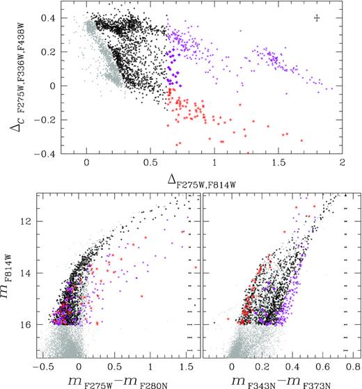
The upper panel of Fig. 5 shows the ChM of ω Cen where the metal-poor stars ([Fe/H]∼−1.8) identified by Milone et al. (2017a) are represented with black dots and coloured grey the remaining stars. The sample of metal-poor stars has been selected on the basis of the fact that it define the reddest RGB sequence in mF336W versus mF336W − mF814W CMD, which is sensitive to stellar populations with different metallicities in Type II GCs (e.g. Marino et al. 2011a, 2015, 2018). The selected metal-poor stars also populate the bluest RGB sequence in CMD made with optical filters (e.g. mF438W versus mF438W − mF814W) and define a distinct sequence in the ChM. Furthermore, the low metallicity of these stars is confirmed by direct spectroscopic measurements of the iron abundance from Johnson & Pilachowski (2010), Marino et al. (2011b), and Mucciarelli et al. (2019). Lower panels highlight metal-poor stars in the mF814W versus mF275W − mF280N and the mF814W versus mF343N − mF373N CMDs. The RGB is clearly split in the left-hand panel CMD and the RGB sequence with redder mF275W − mF280N colours includes ∼30 per cent of the total number of RGB stars. The colour separation between the two main RGBs is about 0.2 mag at mF814W = 16.0 and decreases towards bright luminosities. The two RGBs merge together at mF814W ∼ 12.5.
![This figure illustrates the procedure to identify metal-poor stars in ω Cen. the upper panel reproduces the ΔCF275W, F336W, F438W versus ΔF275W, F814W ChM of ω Cen from Milone et al. (2017a). Lower panels show the mF814W versus mF275W − mF280N (left) and the mF814W versus mF343N − mF373N CMD (right) of ω Cen. Metal-poor stars are marked with black dots. The arrows plotted in the upper panel show the effect of changing He, C, N, O, Mg, and Fe, one at a time, on ΔCF275W, F336W, F438W and ΔF275W, F814W. We adopted an iron variation of Δ[Fe/H] = 0.30 and the same C, N, O, and Mg variations of Fig. 4.](https://oup.silverchair-cdn.com/oup/backfile/Content_public/Journal/mnras/497/3/10.1093_mnras_staa2119/1/m_staa2119fig5.jpeg?Expires=1750414428&Signature=XBxoMJJLcVa5~~ky-m545eB2tNxttp-GlSUUZDL~Gq6lOpFtnXA2lIRPf9fAeknuu3UNedHxFucvrOeTw8jjlmbYBs3R~UNSJW6cW0kOlqrVtB-UALrXKH4djVZkNC~kXNLQrV6330ELBkPg3E8EN~FwgYutiIiRUkagj7RAG0WeRaO1dh1MM-ucaRxucL02oNlU3pf9L~Q~k~~qalF3AI74fMuIX79PRTqJkFHsoQeI-sjUqBXWrSaa8lPCdnrJmytL4-qrxCWAR7kexjmnOog5kHhMBlD6F9eMA7tpDyL4nSGcCaGrBKyhR3BeG1ILQ8C5FGhoQ9HBAVw7F5MBpQ__&Key-Pair-Id=APKAIE5G5CRDK6RD3PGA)
This figure illustrates the procedure to identify metal-poor stars in ω Cen. the upper panel reproduces the ΔCF275W, F336W, F438W versus ΔF275W, F814W ChM of ω Cen from Milone et al. (2017a). Lower panels show the mF814W versus mF275W − mF280N (left) and the mF814W versus mF343N − mF373N CMD (right) of ω Cen. Metal-poor stars are marked with black dots. The arrows plotted in the upper panel show the effect of changing He, C, N, O, Mg, and Fe, one at a time, on ΔCF275W, F336W, F438W and ΔF275W, F814W. We adopted an iron variation of Δ[Fe/H] = 0.30 and the same C, N, O, and Mg variations of Fig. 4.
The discreteness of the various RGB sequences is less evident in the mF814W versus mF343N − mF373N CMD (bottom-right panel of Fig. 5). Metal-poor stars span a colour range of about 0.2 mag in the luminosity interval that ranges from the RGB base to mF814W ∼ 13.5, which is narrower than the mF343N − mF373N spanned by metal-rich stars. The colour spread decreases for mF814W ≲ 13.5 and is comparable with observational errors towards the RGB tip.
5.1 The ΔF343N, F373N versus ΔF275W, F280N chromosome map
The mF814W versus mF275W − mF280N and mF814W versus mF343N − mF373N CMDs plotted in the bottom panels of Fig. 5, are used to derive the ΔF343N, F373N versus ΔF275W, F280N ChM of RGB stars that we plot in Fig. 6 (see Milone et al. 2015, 2018; Zennaro et al. 2019, for details). We only included stars with 13.8 < mF814W < 16.0, which is the magnitude interval where multiple populations are clearly visible.
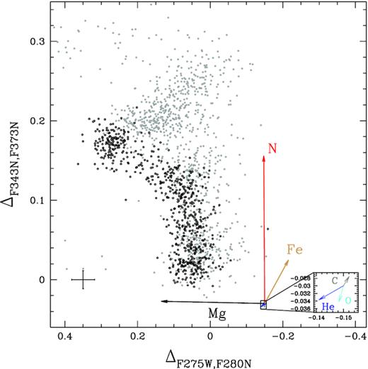
ΔF343N, F373N versus ΔF275W, F280N ChM of RGB stars with 13.8 < mF814W < 16.0. Metal-poor stars are represented with black circles, while the remaining stars are coloured grey. The arrows indicate the effect of changing He, C, N, O, Mg, and Fe, one at a time, on ΔF343N, F373N and ΔF275W, F280N.
Fig. 6 reveals that about 70 per cent of metal-poor stars define a vertical sequence with ΔF275W, F280N ∼ 0.05, while most of the remaining metal-poor stars are clustered around ΔF275W, F280N ∼ 0.3 and ΔF343N, F373N ∼ 0.18. As demonstrated in Section 4.2, the abscissa of this ChM is mostly sensitive to magnesium abundance. Hence, we conclude that about 30 per cent of the selected metal-poor stars in ω Cen are significantly depleted in [Mg/Fe].
Fig. 7 compares the classical ChM of ω Cen from Milone et al. (2017a) with the ΔF275W, F280N versus ΔF343N, F373N ChM introduced in this paper. We used green colours to mark the 1G stars defined by Milone and collaborators, which contains 25.9 ± 1.3 per cent of stars. We also identified four main groups of 2G stars with different values of ΔCF275W, F336W, F438W, that we called 2GA–D and include 20.7 ± 1.2, 23.2 ± 1.3, 6.3 ± 0.7, and 23.8 ± 1.3 per cent of metal-poor stars, respectively. Their stars are represented in Fig. 7 with blue, cyan, orange, and magenta colours, respectively. We find that 2G stars have, on average, higher values of ΔF275W, F280N, and ΔF343N, F373N than 1G stars. 2GA and 2GB stars share almost the same range of ΔF275W, F280N as 1G stars, but have higher ΔF343N, F373N values than the 1G. 2GD stars exhibit significantly higher values of ΔF275W, F280N and ΔF343N, F373N than the remaining RGB stars, while the poorly populated group of 2GC stars exhibits intermediate values of ΔF275W, F280N and ΔF343N, F373N.
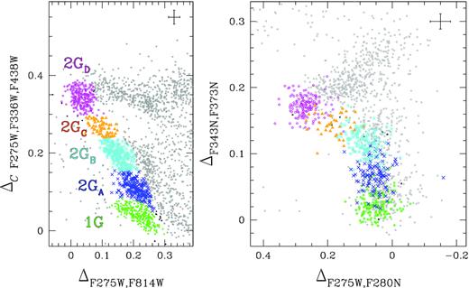
Zoom in of the ΔCF275W, F336W, F438W versus ΔF275W, F814W ChM around the region populated by metal-poor stars (left-hand panel) and ΔF275W, F280N versus ΔF343N, F373N ChM (lower panel) of RGB stars of ω Cen. 1G stars are represented with green symbols, while the groups of 2GA–D metal-poor stars are coloured blue, cyan, orange, and magenta, respectively. Grey dots represent the remaining RGB stars.
Since ΔF275W, F280N quantity is mostly affected by magnesium variation, we conclude that 1G stars share similar [Mg/Fe] as 2GA and 2GB stars and correspond to the populations with [Mg/Fe] ∼ 0.5 identified by Norris & Da Costa (1995), while the remaining stars are significantly depleted in magnesium with respect to the bulk of ω Cen stars, with 2GD stars having the lowest magnesium content. The fact that in monometallic GCs the ΔF343N, F373N quantity is mostly sensitive to nitrogen variations, indicates that the nitrogen abundance increases when we move from the 1G, which has the lowest value of [N/Fe], to 2GD. In the next section, we will exploit photometry in 36 filters to constrain the chemical composition of the metal-poor stellar populations in ω Cen.
5.2 The chemical composition of stellar populations
To infer the relative abundances of He, C, N, O, and Mg between 2GA–D and 1G stars, we extended the method by Milone et al. (2012a, 2018) and Lagioia et al. (2018, 2019) to the sample of metal-poor stars of ω Cen. Briefly, we derived the fiducial lines of 2GA–D and 1G stars in the mF814W versus mX − mF814W CMD in the luminosity interval between mF814W = 13.8 and mF814W = 16.0, where X corresponds to each of the 36 filters used in this paper and listed in Section 2. To do this, we divided the RGB into F814W magnitude intervals of size δm = 0.25 mag which are defined over a grid of points spaced by magnitude δm/2 bins of size. For each bin we calculated the median mF814W magnitude and mX − mF814W colour and linearly interpolated these median points.
As an example, in the upper panels of Fig. 8 we plot mF814W against mX − mF814W for RGB stars of ω Cen, where X = F275W, F280N, F343N, and F438W and use green, blue, cyan, orange, and magenta colours to represent the fiducials of the 1G, 2GA–D.
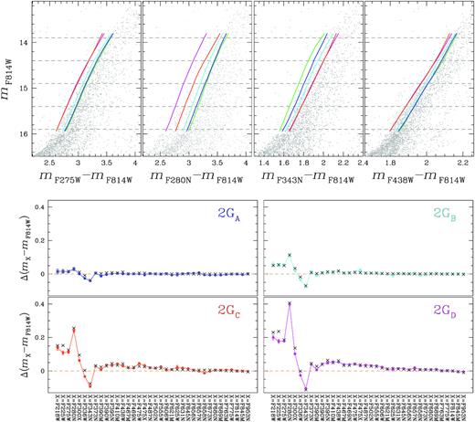
Upper panels show the mF814W versus mX − mF814W CMDs for RGB stars, where X = F275W, F280N, F343N, and F438W. The fiducial lines of the 1G and 2GD populations identified in the paper are coloured green and magenta, respectively, while the dashed lines mark the five values of |$m_{\rm \mathit{ F}814\mathit{ W}}^{\rm CUT}$| used to estimate the relative chemical compositions of the various stellar populations. Lower panels show the mX − mF814W colour differences between the fiducials of 2GA–D stars and the fiducial of 1G stars for the 36 X filters calculated at |$m_{\rm \mathrm{ \mathit{ F}}814\mathrm{ \mathit{ W}}}^{\rm CUT}=15.9$|. Observations are represented with coloured points while black crosses correspond to the best-fitting models. The procedure, illustrated in the lower panels for |$m_{\rm \mathit{ F}814\mathit{ W}}^{\rm CUT}=15.9$| has been extended to the other four values of |$m_{\rm \mathit{ F}814\mathit{ W}}^{\rm CUT}$|.
We defined five reference magnitudes along the RGB, namely |$m^{\rm ref}_{\rm \mathit{ F}814\mathit{ W}}=15.9, 15.4, 14.9, 14.4$|, and 13.9 to derive five estimates of the chemical composition of stellar populations. These five magnitude levels are marked with dashed horizontal lines in the upper panels of Fig. 8. For each value of |$m^{\rm ref}_{\rm \mathit{ F}814\mathit{ W}}$|, we measured the colour difference between the fiducial of 2GA–D and the fiducial of 1G stars (Δ(mX − mF814W)).
We exploited the isochrones by Dotter et al. (2008) that provide the best match with the observed mF814W versus mF606W − mF814W CMD to estimate the gravities and the effective temperatures of 1G stars corresponding to the five reference points. To do this, we assumed [Fe/H] = −1.8, which is similar to the iron abundance inferred by Marino et al. (2019) for metal-poor stars of ω Cen, [α/Fe] = 0.4. We also adopted age of 13.0 Gyr, distance modulus (m − M)0 = 13.58 and reddening E(B− V) = 0.15, which are similar to the quantities provided by Harris (1996, updated as in 2010) and Dotter et al. (2010).
To constrain the chemical composition of 2GA–D stars from the colours calculated at |$m^{\rm ref}_{\rm \mathit{ F}814\mathit{ W}}=15.9$|, we computed a grid of synthetic spectra with different abundances of He, C, N, O, and Mg, that we compare with a synthetic spectrum corresponding to the 1G used as reference. The latter has the values of gravity and effective temperature inferred from the best-fitting isochrone for |$m^{\rm ref}_{\rm \mathit{ F}814\mathit{ W}}=15.9$|, Y = 0.246, [C/Fe] = 0.0, [N/Fe] = 0.0, [O/Fe] = 0.4, and [Mg/Fe] = 0.4. We assumed for synthetic spectra a set of values for [C/Fe] that range from −0.5 to 0.1, [N/Fe] between 0.0 and 1.5, [O/Fe] that ranges from −0.6 to 0.5 and [Mg/Fe] from −0.2 to 0.5. We used steps of 0.05 dex for all elements. The helium mass fractions of the comparison spectra range from Y = 0.246 to 0.400 in steps of 0.001 and the effective parameters of helium-rich isochrones are taken from the corresponding isochrones from Dotter et al. (2008). The spectra are computed by using the computer programs ATLAS 12 and Synthe (Sbordone et al. 2004, 2007; Kurucz 2005; Castelli 2005).
We convoluted each spectrum with the transmission curves of the 36 WFC3/UVIS and ACS/WFC filters available for ω Centauri and derived the colour difference between 2GA–D and 1G stars corresponding to each reference point. The best estimates of Y, C, N, O, and Mg of 2GA–D stars, for |$m^{\rm ref}_{\rm \mathit{ F}814\mathit{ W}}=15.9$| are given by the elemental abundances of the comparison synthetic spectrum that provides the best fit with observed colour differences. The best fit is derived by means of χ-square minimization that is calculated by accounting for the uncertainties on colour determinations and on the sensitivity of the colours to the abundance of a given element, as inferred from synthetic spectra (see Dodge 2008). In the following cases, we excluded some filters to derive the abundances of certain elements. Specifically, we constrained the helium content from filters that are redder than F438W as they are poorly affected by the effect of C, N, O, and Mg on stellar atmosphere. We used the F336W and F343N filters to infer the content of nitrogen alone, as they are largely affected by the abundance of this element. Similarly, we used F280N to derive the magnesium abundance alone. An example is provided in the lower panels of Fig. 8, where we compare the colour differences between the fiducials of 2GA–D stars and the fiducial of the 1G calculated at |$m_{\rm \mathit{ F}814\mathit{ W}}^{\rm cut}=15.9$| (coloured points) with the colour differences from the best-fitting comparison spectra (black crosses).
This procedure, discussed and illustrated for |$m_{\rm \mathit{ F}814\mathit{ W}}^{\rm cut}=15.9$|, is extended to the other four reference magnitudes and provides five determinations of He, C, N, O and Mg of population 2GA–D-stars relative to the 1G. The average abundances are listed in Table 3.
Average abundances of He, C, N, O, and Mg of population 2GA–D-stars relative to the 1G.
| Population | ΔY | Δ[C/Fe] | Δ[N/Fe] | Δ[O/Fe] | Δ[Mg/Fe] |
|---|---|---|---|---|---|
| 2GA | 0.005 ± 0.004 | −0.20 ± 0.08 | 0.31 ± 0.08 | −0.15 ± 0.08 | −0.03 ± 0.04 |
| 2GB | 0.016 ± 0.007 | −0.20 ± 0.09 | 0.62 ± 0.09 | −0.30 ± 0.07 | −0.13 ± 0.06 |
| 2GC | 0.051 ± 0.010 | −0.32 ± 0.11 | 0.75 ± 0.10 | −0.50 ± 0.09 | −0.25 ± 0.07 |
| 2GD | 0.081 ± 0.007 | −0.42 ± 0.08 | 1.02 ± 0.07 | −0.60 ± 0.09 | −0.44 ± 0.06 |
To test the robustness of the results and estimate the uncertainties, we repeated the procedure described above on 1000 simulated mF814W versus mX − mF814W CMDs with fixed light-element variations and the same number of stars and observational errors as our observations of ω Centauri. We find that our procedure correctly recovers the input abundances and provides the uncertainties listed in Table 3.
We find that 2GA and 1G stars have similar magnesium content, while 2GD stars exhibit extreme magnesium depletion by Δ[Mg/Fe] ∼ 0.45 dex, with respect to the 1G. 2GB and 2GC exhibit intermediate magnesium abundances. As shown in Fig. 9, the abundances of helium and nitrogen anticorrelate with magnesium content, while carbon and oxygen correlate with [Mg/Fe]. 2GD stars, which exhibit the largest abundance variations, are enhanced in [N/Fe] by ∼1.0 dex and in helium mass fraction by ∼0.08, with respect to the 1G. Moreover, 2GD stars are depleted in carbon and oxygen by ∼0.4 and ∼0.6 dex, when compared with the 1G. 2GA–C stars exhibit intermediate abundances of He, C, N, and O.
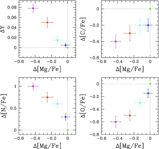
The abundances of helium, carbon, nitrogen, and oxygen of the five studied stellar populations relative to the 1G abundances are plotted against the relative magnesium content. Green, blue, cyan, orange, and magenta colours represent 1G and 2GA − D stellar populations, respectively.
6 METAL-RICH STELLAR POPULATIONS
In this section, we investigate the sample of metal-rich stars identified by Milone et al. (2017a) that we highlight in the ChM and CMDs of Fig. 10. Specifically, we used red and purple symbols to represent the metal-rich stars with ΔF275W, F814W > 0.6, which comprise stars with [Fe/H] ≳ −1.0 (Marino et al. 2019), and we coloured black the remaining metal-rich stars (hereafter metal-intermediate sample).
ΔCF275W, F336W, F438W versus ΔF275W, F814W ChM (upper panel), mF814W versus mF275W − mF280N (left) (lower left panel) and mF814W versus mF343N − mF373N CMD (lower right panel) of ω Cen. Metal-rich stars with ΔF275W, F814W < 0.65 are coloured black. The remaining metal-rich stars of the lower, middle, and upper stream are represented with red starred symbols, purple diamonds, and purple crosses, respectively.
The RGBs of metal-rich stars clearly exhibit less-steep slopes than those of metal-poor and metal-intermediate stars in the mF814W versus mF275W − mF280N, in qualitative agreement with the isochrones plotted in Fig. 3. Metal intermediate stars with mF814W > 13.8 span a smaller range of mF275W − mF280N than metal-poor stars with similar F814W magnitude. Moreover, there is no clear evidence for a bimodal mF275W − mF280N distribution as observed for metal-poor stars.
Based on chemical abundances of stars in the ChM, Marino et al. (2019) identified the lower, middle, and upper streams that are composed of N-poor, N-intermediate, and N-rich stars, respectively. The sample of metal-intermediate stars with mF814W ≳ 13.5 is shown in Fig. 10 span an interval of ∼0.1 mag in mF343N − mF373N and is composed of three main RGBs. The RGB with the reddest mF343N − mF373N colour is the most-populated one and is composed of stars of the upper stream of ω Cen. The bluest and the middle RGBs comprise stars that populated the lower and the middle stream.
Stars in the lower, middle, and upper stream with ΔF275W, F814W > 0.65 are represented with red starred symbols, purple diamonds, and purple crosses, respectively. Most of these metal-rich stars are distributed into two distinct sequences that define the bluest and the reddest boundaries of the low RGB in the mF814W versus mF343N − mF373N CMD, and are composed of stars of the lower and upper stream, respectively. Middle stream stars exhibit intermediate colours. All metal-rich stars exhibit bluer mF343N − mF373N colours than the remaining RGB stars at magnitudes brighter than mF814W ∼ 13.0, as expected from isochrones with different metallicities (see Fig. 3).
The fact that metal-intermediate and metal-rich stars of ω Cen span a wide metallicity interval makes it challenging to estimate their relative abundances of He, C, N, O, and Mg. Indeed, the method adopted in Section 5.2 for metal-poor stars is based on the comparison between the observed colours of multiple populations and the colours derived by synthetic spectra with appropriate chemical composition. Metallicity variations, including iron abundance and overall C+N+O abundances, provide significant changes on stellar structure (Sbordone et al. 2011), thus affecting the atmospheric parameters of synthetic spectra. Nevertheless, metallicity is poorly constrained for the various stellar populations of ω Cen (Marino et al. 2019).
For this reason, we will only provide a qualitative discussion on the chemical composition of metal-intermediate and metal-rich stellar populations, which are strongly enhanced in [Fe/H] and [(C+N+O)/Fe] with respect to metal-poor stars (e.g. Johnson & Pilachowski 2010; Marino et al. 2011b, 2012).
To do this, we reproduce in the upper left panel of Fig. 11 the ΔF343N, F373N versus ΔF275W, F280N ChM and highlight metal-intermediate and metal-rich stars with black and purple + red symbols, respectively. Most metal-rich stars define two horizontal sequences with nearly constant ΔF343N, F373N ∼ 0.0 (populated by lower stream stars) and one with ΔF343N, F373N ∼ 0.3 that hosts upper stream stars. Middle stream metal-rich stars exhibit intermediate ΔF343N, F373N values.
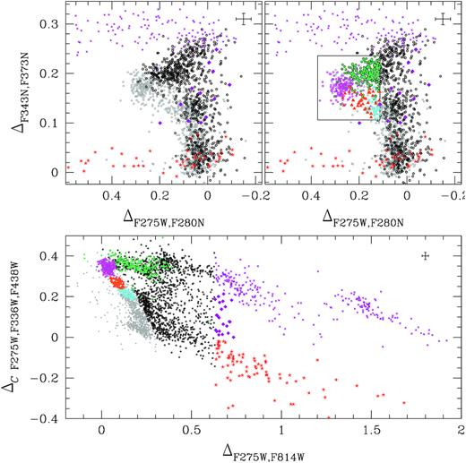
Upper-left panels. Reproductions of the ΔF343N, F373N versus ΔF275W, F280N ChM introduced in Fig. 6. We used black colours to represent the metal-intermediate stars defined in Fig. 10 while metal-rich stars that belong to the upper, middle, and lower stream are represented with purple crosses, purple diamonds, and red starred symbols, respectively. The remaining RGB stars are coloured grey. The box superimposed on the ChM plotted in the upper right panel encloses stars with depleted magnesium. Lower panel. ΔCF275W, F336W, F438W versus ΔF275W, F814W ChM. The 2GB, 2GC, and 2GD metal-poor stars within the box shown in the upper left panel are coloured cyan, orange, and magenta, respectively, while candidate Mg-poor metal-intermediate stars marked with aqua symbols in the upper left and lower panels.
Metal-intermediate stars define three main stellar blobs with ΔF275W, F280N ∼ 0.05 but different values of ΔF343N, F373N ∼ 0.05, 0.13, and 0.20 that we indicate as M-IA, M-IB, and M-IC, respectively, and are composed of stars in the lower, middle, and upper stream. A fourth group of metal-intermediate stars (M-ID) is distributed around (ΔF275W, F280N: ΔF343N, F373N) ∼ (0.15:0.20).
To highlight metal-poor and metal-intermediate stars that, based on their position in the ΔF343N, F373N versus ΔF275W, F280N ChM, are strongly depleted in magnesium with respect to the majority of ω Cen stars, we draw the grey box in the upper right panel of Fig. 11. This box includes the metal-poor populations 2GC and 2GD that we represented with magenta and orange points, respectively, plus a few population 2GB stars coloured cyan. The evidence that the M-ID stars in the box (aqua dots) have larger values of ΔF275W, F280N than the Mg-rich metal-poor stars demonstrate that they have low-magnesium content.
The ΔCF275W, F336W, F438W versus ΔF275W, F814W ChM plotted in the lower panel of Fig. 11 reveals that metal-intermediate Mg-poor stars belong to the upper stream. Hence, as shown by Marino et al. (2019), they have enhanced He, N, and Na and depleted C and O.
7 SUMMARY AND DISCUSSION
We exploited high-precision photometry in the F275W, F280N, F343N, and F373N bands of HST of ω Centauri, to introduce a ChM that is able to identify stellar populations with different Mg and N abundances along the RGB. Based on synthetic spectra with appropriate light-element abundances, we demonstrated that the abscissa of this new ChM, ΔF275W, F280N, is mostly sensitive to the relative content of magnesium of the stellar populations of monometallic GCs and is poorly affected by star-to-star variations of He, C, N, and O. Its ordinate, ΔF343N, F373N, maximizes the separation between stellar populations with different nitrogen and is negligibly affected by variation in the other light elements involved in the multiple population phenomenon, including He, C, O, and Mg. In GCs with iron variations, both axes of the ΔF343N, F373N versus ΔF275W, F280N are affected by changes in metallicity.
To constrain the chemical composition of stellar populations in ω Cen, we first considered the sample of metal-poor stars identified by Milone et al. (2017a) on the ΔCF275W, F336W, F438W versus ΔF275W, F814W ChM, which comprises stars with nearly homogeneous [Fe/H] (Marino et al. 2019). We separated 1G and 2G stars as in Milone et al. (2017a) and selected four main groups of 2GA–2GD stars that span different intervals of ΔCF275W, F336W, F438W. 1G stars and 2GA–2GD stars include 25.9 ± 1.3 per cent, 20.7 ± 1.2 per cent, 23.2 ± 1.3 per cent, 6.3 ± 0.7 per cent, and 23.8 ± 1.3 per cent, respectively, of the total number of studied metal-poor RGB stars.
As expected, the average ΔF343N, F373N increases from 1G- to 2GD-stars. Indeed, both ΔF343N, F373N and ΔCF275W, F336W, F438W strongly depend on the nitrogen abundance. The fact that population 2GA exhibits similar values of ΔF275W, F280N as 1G stars shows that these populations share similar magnesium abundances. The high values of ΔF275W, F280N of 2GD stars are indicative of their high depletion in [Mg/Fe], while 2GC and 2GB stars have intermediate magnesium abundances.
We exploited photometry collected through 36 filters of ACS/WFC and WFC3/UVIS on board HST and compared the relative colours of the various populations with the colours derived from synthetic spectra with appropriate chemical compositions. We thus inferred the abundances of He, C, N, O, and Mg of 2GA–D stars relative to the 1G. We find that 2GA stars have nearly the same magnesium abundance as the 1G, while 2GB, 2GC, and 2GD stars are depleted in magnesium by ∼0.15, ∼0.25, and ∼0.45 dex, respectively.
All 2G stars are more helium- and nitrogen-rich than 1G stars, with 2GD stars having the highest enhancement of both elements (ΔY ∼ 0.08 and Δ[N/Fe] ∼ 1.0). The second generations have lower content of carbon and oxygen than the 1G, with 2GD stars having extreme contents of these elements. These results show that the magnesium content of the populations of ω Cen correlates with the abundances of oxygen and carbon and anticorrelates with helium and nitrogen. These correlations are interpreted as the result of proton-capture nucleosynthesis in the CNO cycle and the MgAl chain of H-burning. In particular, the MgAl chain, which is responsible for magnesium variations is only active at temperatures higher than ∼7 × 10⁷ K (e.g. Denisenkov & Denisenkova 1990; Langer, Hoffman & Sneden 1993; Prantzos & Charbonnel 2006; Renzini et al. 2015; Prantzos, Charbonnel & Iliadis 2017). Clearly, the material making the Mg-poor populations was exposed to higher temperatures than the Mg-rich stars, with p-captures having destroyed Mg making Al.
We find that about 70 per cent of the selected metal-intermediate stars of ω Cen exhibit similar values of ΔF275W, F280N but are clustred around three different values ΔF343N, F373N. We verified that these three groups of stars populate the lower, middle, and upper streams defined by Marino et al. (2019) and are composed of stars with different nitrogen contents. Accurate estimates of the magnesium abundance of metal-intermediate and metal-rich stars of ω Cen are challenged by the internal variation of [Fe/H] in these stars. Nevertheless, the fact that a sample of metal-intermediate stars exhibit larger values of ΔF275W, F280N than Mg-rich metal-poor stars indicates that they are depleted in [Mg/Fe].
Norris & Da Costa (1995) determined abundances of magnesium and of other 19 elements for 40 RGB stars of ω Cen, based on high-resolution spectroscopy. They find that the majority of stars have nearly constant [Mg/Fe] ∼ 0.4, with the exception of five stars where magnesium is clearly underabundant ([Mg/Fe] ∼ −0.1). Two Mg-depleted stars have [Fe/H] ∼ −1.7 while the other three have slightly higher iron abundances of [Fe/H] ∼ −1.5. Hence, the group of Mg-depleted stars populate the metal-poor portion of the [Fe/H] distribution of the stars analysed by Norris & Da Costa (1995), which span the interval −1.8 ≲ [Fe/H] ≲ −0.8. Norris & Da Costa (1995) noticed that a common property of the group is that it includes only CN-rich and Al-rich stars and that four out five stars are strongly oxygen depleted.
Although HST photometry is not available for the stars studied by Norris & Da Costa (1995), their findings that the metal-poor population of ω Cen hosts stars depleted by ∼0.5 dex in [Mg/Fe] with respect to the bulk of metal-poor stars and that the metal-intermediate stars also host stars with low magnesium abundances are consistent with the conclusions of our paper. The evidence that ω Cen hosts stars with depleted magnesium has been recently confirmed by Mészáros et al. (2020) based on spectra of 898 stars collected by the APOGEE survey. These results, based on high-resolution spectroscopy, demonstrate that the ΔCF275W, F336W, F438W versus ΔF275W, F814W ChM introduced in this work, is an efficient tool to disentangle stellar populations with different [Mg/Fe] and infer their magnesium abundances.
ACKNOWLEDGEMENTS
We are grateful to the anonymous referee for a constructive report that has improved the quality of the manuscript. This work has received funding from the European Research Council (ERC) under the European Union’s Horizon 2020 research innovation programme (Grant Agreement ERC-StG 2016, No 716082 ‘GALFOR’, PI: Milone, http://progetti.dfa.unipd.it/GALFOR), and the European Union’s Horizon 2020 research and innovation programme under the Marie Sklodowska-Curie (Grant Agreement No 797100, beneficiary Marino). APM, MT, and ED acknowledge support from Ministero dell'innovazione, universita' e ricerca (MIUR) through the FARE project R164RM93XW SEMPLICE (PI: Milone). APM and MT have been supported by MIUR under PRIN program 2017Z2HSMF (PI: Bedin). C L ȧcknowledges support from the one-hundred-talent project of Sun Yat-set University. CL was supported by the National Natural Science Foundation of China under grants 11803048. This work is based on observations made with the National Aeronautics and Space Administration (NASA)/European Space Agency (ESA) Hubble Space Telescope, obtained from data archive at the Space Telescope Science Institute (STScI). STScI is operated by the Association of Universities for Research in Astronomy, Inc. under NASA contract NAS 5-26555.
DATA AVAILABILITY
The data underlying this article will be shared on reasonable request to the corresponding author.
