


ABSTRACT
The conventional approach to orbit trapping at Lindblad resonances via a pendulum equation fails when the parent of the trapped orbits is too circular. The problem is explained and resolved in the context of the Torus Mapper and a realistic Galaxy model. Tori are computed for orbits trapped at both the inner and outer Lindblad resonances of our Galaxy. At the outer Lindblad resonance, orbits are quasi-periodic and can be accurately fitted by torus mapping. At the inner Lindblad resonance, orbits are significantly chaotic although far from ergodic, and each orbit explores a small range of tori obtained by torus mapping.
1 INTRODUCTION
It has long been recognized that angle-action variables, |$({\boldsymbol \theta },{\bf J})$| are valuable tools for galactic dynamics (e.g. Lynden-Bell & Kalnajs 1972; Kalnajs 1977; Weinberg 2001). Over the last decade, the use of angle-action variables has become more widespread on account of the arrival of algorithms for computing the transformation between these rather abstract variables and ordinary phase-space variables (x, v). All these algorithms derive from our ability to solve the Hamilton–Jacobi equation for the Stäckel potentials (de Zeeuw 1985) or limiting cases of them, but a variety of stratagems make it possible to obtain good approximations to angle-action coordinates for most plausible galactic potentials. One stratagem is the Stäckel Fudge (Binney 2012; Sanders & Binney 2015), another is torus mapping (Binney & McMillan 2016, and references therein), and a third is construction of the generating function by orbit integration (Sanders & Binney 2014). These techniques are all limited to orbits that are qualitatively the same as orbits supported by Stäckel potentials.
The phenomenon of resonant trapping gives rise to orbits in real potentials that are qualitatively different from any orbit in a Stäckel potential, and we have reason to believe that such orbits are astronomically important (e.g. Dehnen 2000; Monari et al. 2017; Pérez-Villegas et al. 2017). Binney (2018, hereafter B18) gave algorithms for the construction of angle-action variables for orbits that are trapped at the principal resonances of a realistic model of the Galaxy’s bar. The paper focused of trapping at the corotation and outer Lindblad resonances (OLRs), but its approach is more widely applicable. Indeed, the code released with the paper was directly applicable to orbits trapped at the inner Lindblad resonance (ILR). C++ code that computes tori trapped at the principal resonances of a disc was released in the form of an upgrade to the Torus Mapper (hereafter tm) (Binney & McMillan 2016).
In the course of a study of signatures of resonant trapping in velocity space at the Sun (Binney 2020), it emerged that the standard approach adopted by B18 fails for certain nearly circular orbits. The principal aim of this paper is to explain what this problem is, and to show how it can be solved. The performance of the version of tm that resolves this problem is illustrated by tori that straddle the standard and new regimes at both the ILR and OLR.
Paper is organised as follows. Section 2 specifies the model of the Galactic disc and bar that is employed. Section 3 explains why the standard pendulum equation relied on by B18 breaks down and presents a more robust algorithm. Section 4 applies the new algorithm to orbits trapped at OLR, while Section 5 applies it to orbits trapped at the ILR. Section 6 connects the angle-action approach to elementary theory of perturbed orbits, and Section 7 sums up.
2 THE POTENTIAL AND UNITS
Sormani, Binney & Magorrian (2015, hereafter S15) constrained the bar’s contribution to Φ with hydrodynamical simulations of the flow of gas in the Galactic plane; these simulations yielded longitude–velocity plots that could be compared with observations in the |$21\,$| cm and |$2.6\,$| mm lines of hydrogen and CO. S15 adopted a simple functional form for ρ and obtained Φ2 by integrating Poisson’s equation. B18 did not use the resulting potential directly but instead adopted a simple functional form for Φ2, derived the corresponding density from ρ = (4πG)−1∇2Φ and chose the strength of the quadrupole component so that at large R it matched that of S15. This procedure guarantees good agreement between the B18 and S15 potentials at the OLR, but allows significant disparity between the potentials at the ILR. Since we here present results at the ILR as well as the OLR, it is important to compare the non-axisymmetric forces implied by each bar model as a function of radius. Fig. 1 does that by showing the circular-speed curve from the axisymmetric model alongside the azimuthal analogues, (∂Φ2/∂ϕ)1/2, from the two bar models. These agree by construction at large R, but at small R the S15 curve peaks sooner and higher.
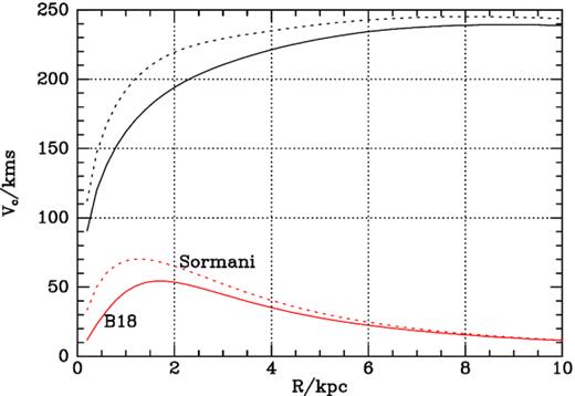
Full black curve: circular-speed of the ‘best’ potential of McMillan (2011). Dotted black curve: circular-speed of an axisymmetric potential that is consistent with the existence of x2 orbits in combination with the S15 bar. Full red curve: (∂Φ2/∂ϕ)1/2 from the B18 bar model. Dashed red curve (∂Φ2/∂ϕ)1/2 from the S15 bar model.
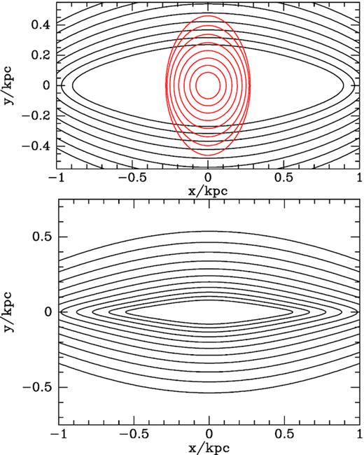
Fig. 2 shows the closed orbits in these two model potentials. The greater quadrupole strength of the S15 potential at small radii makes the x1 orbits (plotted in black) more elongated than in the B18 model, and completely eliminates the x2 orbits (plotted in red). A viable bar model requires x2 orbits because dense gas moving on these orbits forms the heart of the Central Molecular Zone (e.g. Ferrière, Gillard & Jean 2007). Fig. 3 shows closed orbits when the S15 bar model is combined with an axisymmetric model that has a more massive bulge and therefore a more steeply rising circular speed curve. The full black curve in the top panel of Fig. 1 shows the circular speed curve of the McMillan (2011) potential that does not produce x2 orbits when combined with the S15 bar, while the black dashed curve shows a more steeply rising circular speed curve obtained by increasing the central density of the bulge from 9.56 to |$15.6\times 10^{10}\, {\rm M}_\odot \, \mathrm{kpc}^{-3}$|. Fig. 3 shows that with the more massive bulge the S15 bar permits x2 orbits.

2.1 Units
In tm the natural unit of distance is kpc and the natural unit of velocity is |$\, \mathrm{kpc}\, \mathrm{Myr}^{-1}=978\, \mathrm{km\, s}^{-1}$|, with the consequence that the natural units of frequency and action are |$\, \mathrm{Myr}^{-1}$| and |$\, \mathrm{kpc}^2\, \mathrm{Myr}^{-1}$|, respectively. In the following units will not be given on the understanding that quantities are expressed in tm’s natural units.
3 MOTION IN THE SLOW PLANE
3.1 The problem
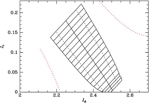
Orbits trapped at the OLR in action space. The centre line of the ladder marks the actions of orbits that satisfy the OLR resonant condition Ωr= 2(Ωp − Ωϕ) in the axisymmetric potential. The ladder is bounded by the extremes of the unperturbed actions that are reached by orbits trapped at OLR. The dashed lines within the ladder show the actions of orbits that just circulate inside or outside OLR. The red dashed lines show the predictions of the classical pendulum equation for the extremes in actions achieved by trapped orbits.
The underlying mathematical problem is this. Orbit-averaging of the Hamiltonian H essentially reduces the dynamics to motion in the slow plane. In the case of the OLR, the natural coordinates for this plane are |$J_1^{\prime }=J_\mathrm{ r}$| and |$\theta _1^{\prime }=\theta _\mathrm{ r}+2\theta _\phi$|. The standard argument is that the difference |$\Delta \equiv J_1^{\prime }-J_{1\, \rm res}^{\prime }$| between the current slow action and that of the perfectly resonant torus satisfies a modified pendulum equation, and if |$J_{1\, \rm res}^{\prime }$| is sufficiently small, the amplitude of the pendulum’s oscillations can be large enough to make |$J_{1\, \rm res}^{\prime }+\Delta \lt 0$|. Given that this problem arises in the regime of nearly circular orbits, in which the classical epicycle approximation should apply, it cannot define a fundamental problem with the use of linear theory, but must arise from a removable cause.
3.2 The solution
The problem is the coordinate singularity at the origin of the |$(J_1^{\prime },\theta _1^{\prime })$| phase plane. At sufficiently large |$J_{1\, \rm res}^{\prime }$|, the motion in |$(\theta _1^{\prime },J_1^{\prime })$| is confined to an annulus that has the origin |$J_1^{\prime }=0$| within it. As |$J_{1\, \rm res}^{\prime }$| is reduced, the mean radius of the annulus diminishes and eventually the hole at its centre disappears. Then the dynamics plays out in a disc that encompasses the origin and we need to move to coordinates that are not singular there.
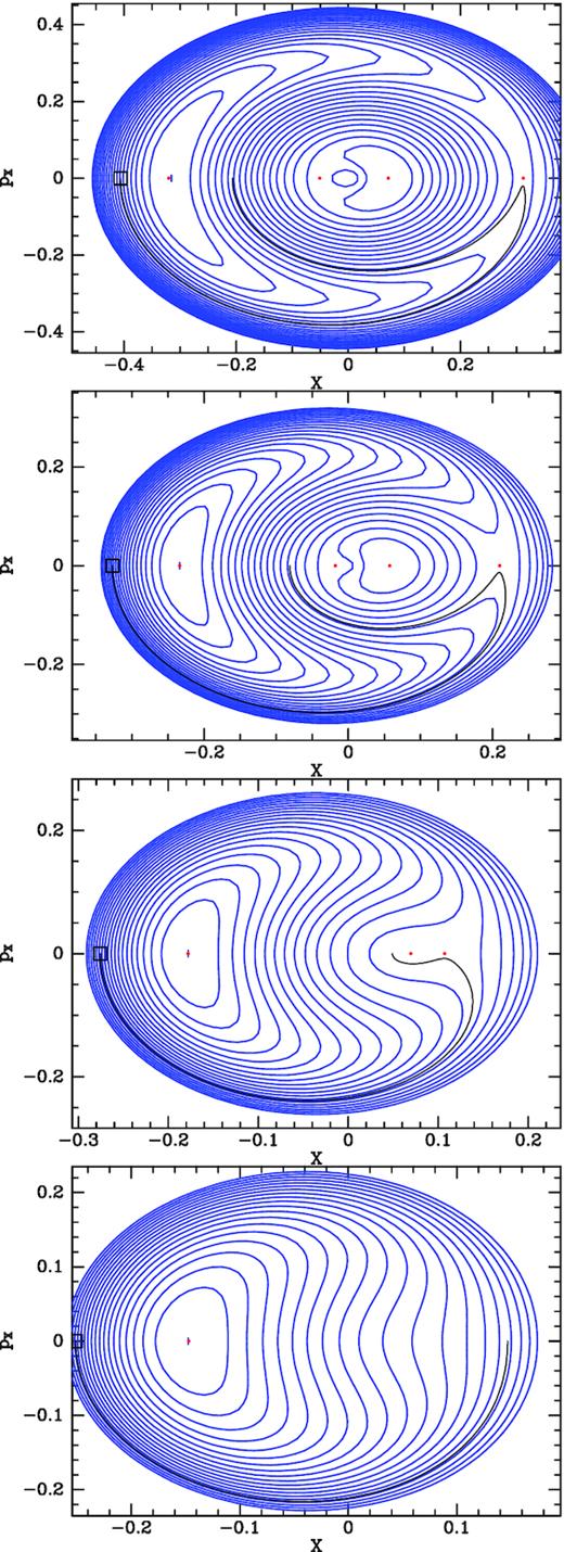
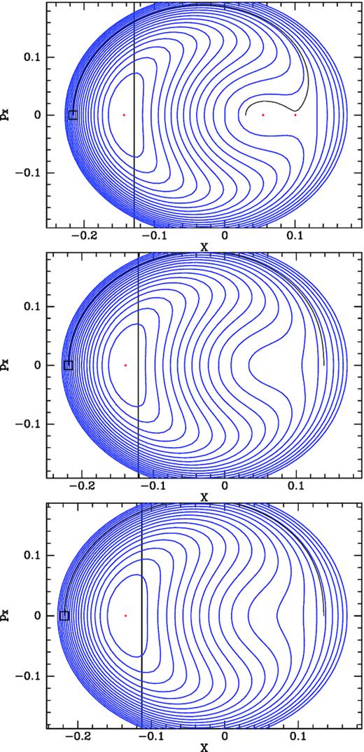
Contours of constant |$H(\theta _1^{\prime },J_1^{\prime })$| when |$J_{1\, \rm res}^{\prime }$| is diminished by factors of 2 from |$J_{1\, \rm res}^{\prime }=0.05$| (top) to 0.00625 (bottom) in the coordinates defined by equations (12). Each panel corresponds to a rung of the ladder in Fig. 4, with the upper panels corresponding to higher rungs than the lower panels. H(X, pX) is computed using quartics in |$\xi =\sqrt{2J_1^{\prime }}$| to fit |$H_0(J_1^{\prime })$| and |$h_N(J_1^{\prime })$|. The black contours are trajectories obtained by integrating Hamilton’s equation in the slow plane to define the tori with the largest possible actions of libration.
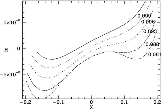
In the top panel the annulus has mean radius ∼0.3 and is occupied by crescent-shaped contours that enclose a stationary point marked by a red dot at X ≃ −0.3. The outermost crescent almost touches itself at the stationary point marked by a red dot on the right at X ≃ 0.3. Fig. 6 shows the value of H along the X axes of the four panels of Fig. 5. We see that the stationary points on the left Fig. 5 are mountain tops, while that stationary points on the right of the upper panels are saddle points; in the top two panels of Fig. 5 a lake bottom lies between these features. As |$J_{1\, \rm res}^{\prime }$| falls, the lake becomes less deep, and eventually its bottom annihilates with the saddle point, so one is left with a mountain that has a steep left-hand face while allowing a fairly easy ascent from the right.
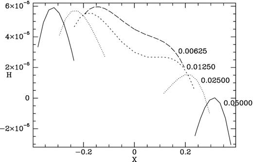
The values of H across the centres of each panel of Fig. 5. Each panel corresponds to a rung of the ladder shown in Fig. 4 and the corresponding curve is labelled by the value of Jr at which its rung crosses the ladder’s centre line. For clarity the curve for Jr = 0.025 is displaced upwards by 10−5, that for Jr = 0.0125 by 2 × 10−5, etc.
This annihilation occurs at the value of |$J_3^{\prime }$| of the rung that first touches the Jϕ axis in Fig. 4. Rungs higher up the ladder terminate at the edge of the ladder, leaving space between their ends, and the Jϕ axis for orbits that circulate inside OLR.
The values of H plotted in Figs 5 and 6 were computed as follows:
The complete Hamiltonian was Fourier analysed on the perfectly resonant torus |$J_{1\, \rm res}^{\prime }$|, and on tori with slightly smaller and larger values of |$J_1^{\prime }$|. As Jr changed along this sequence, Jϕ was adjusted to hold constant |$J_3^{\prime }$|. From the Fourier amplitude H0 for vanishing wavenumber and that, hN, for the resonant wavenumber, the coefficients of the terms appearing in the standard pendulum equation were determined.
The pendulum equation then yielded estimates of the smallest and largest values of |$J_1^{\prime }$| reached by the pendulum when it liberates with maximum amplitude. The dashed red curves in Fig. 4 show these limiting values; they are evidently excessive so are reduced by a factor 0.7. If the smallest value, |$J_{1\, \rm min}^{\prime }$|, was predicted to be negative, it was replaced by a tiny positive value.
- The Hamiltonian was then Fourier analysed on nine tori that had values of |$J_1^{\prime }$| that spanned the range |$(J_{1\, \rm min}^{\prime },J_{1\, \rm max}^{\prime })$| with Jϕ again adjusted to hold constant |$J_3^{\prime }$|. The data for the amplitudes |$H_0(J_1^{\prime })$| and |$h_N(J_1^{\prime })$| obtained in this way, which are plotted in Fig. 6, were fitted by quartics in ξ (equation 13). In B18, by contrast, these amplitudes were fitted by quadratics inThe use of ξ rather than Δ as the independent variable is partly motivated by equation (12), and partly by the consideration that as |$J_1^{\prime }\rightarrow 0$|, smoothness of H(X, pX) near the origin requires that hN ∼ ξ because it is a dipole amplitude. The need for quartics is indicated by the data in Fig. 6 for Jr = 0.0125 shown by the short-dashed curve: in addition to a local maximum at X ∼ −1.9 the curve has a point of inflection near the origin. This structure cannot be fitted by a quadratic.(14)$$\begin{eqnarray*} \Delta \equiv J_1^{\prime }-J_{1\, \rm res}^{\prime }. \end{eqnarray*}$$
Given that hN(0) = 0, the quartic fitted to the data for hN should have no constant term. The quartic fitted to the data for H0 can be similarly specialized since we know that |$0=\partial H_0/\partial J_1^{\prime }$| at |$J_{1\, \rm res}^{\prime }$|.
The quartic in ξ is fitted to data that covers a region only slightly bigger than the annuli in Fig. 5 within which orbits can be trapped. Consequently, no significance should be attached to the quartic’s values well outside this region. In particular, the bumps in the bottom of the lake that feature in the top two panels of Fig. 5 are of no significance.
The effective Hamiltonian that is plotted in the bottom panel of Fig. 5 has only one critical value, namely the value of its maximum, which characterizes the orbit that has vanishing action of libration. A value is adopted as a minimum that creates orbits that effectively circulate around the origin of the |$(\theta _1^{\prime },J_1^{\prime })$| plane. This arbitrarily chosen value sets the upper boundary of the lower rungs in Fig. 4.
3.3 Scope of the problem
The problem solved here is liable to arise in many Hamiltonian systems, in fact whenever a powerful resonance occurs on an unperturbed orbit that has a small action. The corotation resonance is an exception to this rule because in that case the only action involved in the slow plane is Jϕ, which is inherently large. Galactic resonances involving the vertical action, such as the 1:1 resonance between radial and vertical oscillations of stars (Sridhar & Touma 1996; Binney 2016) may give rise to this problem through the smallness of Jz. The approach explained here should always resolve the problem.
4 ORBITS TRAPPED AT OLR
Each panel of Fig. 7 shows cross-sections through five orbits trapped at OLR. The full red curves are computed from an object returned by resTorus_L and calling its method SOS for five values of I between Imin and Imax. The black dots are consequents obtained by integrating the full equations of motion with a fourth-order Runge–Kutta routine starting from one point on three of the full curves. The dashed blue curves are cross-sections through some of the axisymmetric tori that underlie the computation and are drawn by the method SOS of the corresponding Torus object. The fit between the dots and the full curves is almost perfect except where the curves cross the R-axis on the left. The worst errors occur between the smallest and next smallest blue curves in the lower panel, and reflect unresolved issues regarding interpolating between tori that require a point transformation (appendix A3 of Binney & McMillan 2016).
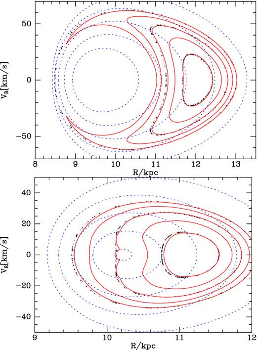
Orbits trapped at OLR in surfaces of section for Jr = 0.05 (upper) and Jr = 0.006 25 (lower) panels. The full red curves are computed by resonant perturbation theory while the black dots are obtained by Runge–Kutta integration of the full equations of motion. The dashed blue curves are cross-sections of some of the axisymmetric tori that underlie the perturbation theory.
The upper panel of Fig. 7 corresponds to the top panel of Fig. 5. At this value of |$J_3^{\prime }=J_\phi -2J_\mathrm{ r}$| the range in Jr over which orbits librate has a lower as well as an upper bound. Orbits with small Jr circulate in |$\theta _1^{\prime }$| too fast to be trapped, while orbits with largest Jr circulate too fast the opposite direction to be trapped. In Fig. 7, the horns of the crescents reach round to touch each other, enclosing an island of blue dashed ovals associated with circulating orbits with small Jr. In the top panel of Fig. 5 these circulating orbits move along ovals that cut the positive X-axis to the left of the saddle point; they tour the lake.
The lower panel of Fig. 7 corresponds to the bottom panel of Fig. 5. At this small value of |$J_3^{\prime }$|, |$\theta _1^{\prime }$| circulates so slowly in the axisymmetric potential that the bar traps the orbit, even at negligible radial action. Hence only orbits with large Jr circulate, so in the bottom panel of Fig. 5 there are no small ovals centred on the origin, and in Fig. 7 the origin lies within the domain of red invariant curves that encircle |$R\sim 11.3\, \mathrm{kpc}$|.
In the bottom two panels of Fig. 5 the distinction between trapped and untrapped orbits has become unclear. The smallest ovals in Fig. 5 describe orbits that keep close to an unperturbed orbit with a particular value of Jr (marked by the red dot) that fails to precess as it would in the underlying axisymmetric potential. As one moves out to larger ovals, the corresponding orbit cycles through a range of values of Jr that at first widens until it embraces the circular orbit Jr = 0. Later the range gradually contracts while its centre shifts to high values of Jr; this contraction is signalled in Fig. 5 by the outer ovals becoming more nearly centred on the origin. During the widening stage, the orbit’s major axis oscillates with increasing amplitude synchronously with variation in its eccentricity. During the contracting stage, the major axis precesses with growing steadiness as the orbit becomes more eccentric. Thus the transition from absolute confinement (at the red dot) to motion very close to that expected in the absence of the bar, is continuous.
As a consequence of this continuity, the lower rungs of the ladder of Fig. 4 do not have unambiguous upper ends. The upper ends of the higher rungs are, by contrast, clearly defined by the value of |${\cal J}$| at which circulation sets in. In Fig. 4, this ambiguity manifests itself in a slight kink in the ladder’s top boundary, which has been set arbitrarily.
5 TRAPPING AT THE ILR
The non-axisymmetric part of the potential becomes more prominent relative to the axisymmetric part as one moves towards the Galactic Centre, with the consequence that in a given bar, perturbation theory works less well for orbits trapped at the ILR than at the OLR. This being so, results are presented for bars that are weaker than that studied at the OLR. In fact, we will use B18 bar with amplitude multiplied by a factor |${\tt Bstrength}\lt 1$|.
The ILR is defined by the vector N = (1, 0, −2). Whereas at the OLR, an axisymmetric, perfectly resonant torus yields G < 0 and ψN = π, at the ILR G > 0 and ψN = 0. Libration is still around |$\theta _1^{\prime }=\pi$|, but now stars move around a minimum rather than a maximum in H.
Fig. 8 shows the orbital structure of a very weak bar: |${\tt Bstrength=0.005}$|. The top panel shows closed orbits. Two orbit families are evident. At radii larger than |$\sim 0.7\, \mathrm{kpc}$| the orbits belong to the x1 family in the notation of Contopoulos & Papayannopoulos (1980), while interior to |$0.7\, \mathrm{kpc}$| the obits (shown in red) belong to the x2 family. The centre panel of Fig. 8 shows contours of the effective Hamiltonian in the slow plane analogous to Fig. 5. The structure is qualitatively the same as that in the top panel of Fig. 5. On the left, crescent shaped contours are followed by orbits that are trapped, while on the far right a saddle point sets the boundary between trapped and untrapped orbits. The only difference between this situation and that at the OLR is that now we have a lake rather than a mountain on the left and a hill rather than a lake near the centre.
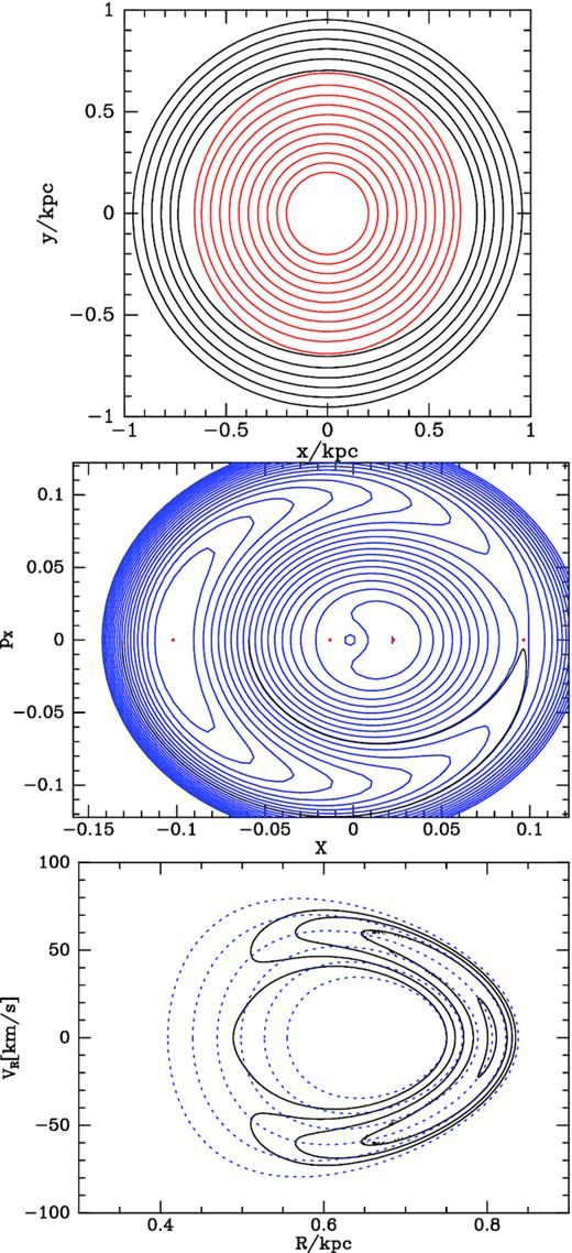
Trapping at the ILR of a weak bar: Bstrength = 0.005 The lower two panels are for Jr = 0.005.
Fig. 9 shows the (Jϕ, Jr) plane in the vicinity of the ILR for bars with strengths that increase from top to bottom from 0.005 to 0.1. The ladder in the bottom panel includes tori with Jr/Jϕ as large as 0.77 even though the bar has only a tenth of the strength of the B18 bar, and less than a tenth the strength of the S15 bar. Tori with larger ratios Jr/Jϕ are costly to compute. Moreover, we shall find that even in this bar trapped orbits are significantly stochastic and are thus pushing the concept of an invariant torus to its limit. For this reason in this section we restrict discussion to |${\tt Bstrength}\le 0.1$|.
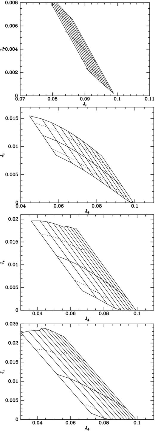
Orbits trapped at the ILR in bars of increasing strength: from top to bottom Bstrength = 0.005, 0.015, 0.05, and 0.1.
Like the OLR’s ladder in Fig. 4, the ladders in Fig. 9 slope from lower right to upper left, but their rungs slope in the same sense as the ladder rather than in the opposite sense. Again the higher rungs finish on the lower boundary of the ladder, leaving room between that point and the Jϕ axis for orbits to circulate inside the ILR, while the lower rungs reach the Jϕ axis. As the strength of the bar grows, the ladder becomes wider and area of the (Jϕ, Jr) plane available to orbits that circulate inside the ILR shrinks dramatically. As the ladder widens, the eccentricity of orbits along its upper edge increases and computing their tori becomes increasingly costly.
The ladders of Fig. 9 have marked kinks in their upper boundaries at the last rung to start from the Jϕ axis. These kinks reflect the fact that once the saddle point has disappeared from the Hamiltonian in the slow plane, the transition from libration to circulation occurs continuously rather than at a well-defined value of |${\cal J}$|, so the upper ends of rungs have to be set arbitrarily.
Fig. 10 is the analogue of Fig. 5 for the ILR of a bar of strength 0.1. The similarity between Fig. 10 and the bottom two panels of Fig. 5 is striking. In the lowest panels of both figures there is a continuous transition between trapped and untrapped orbits. At both the ILR and the OLR, a clear distinction emerges where the ladder’s lower edge reaches the Jϕ axis. In Fig. 10, the rung from this junction corresponds to the middle panel, where the hill is annihilating with the saddle point. Fig. 11 makes this evolution clearer by showing the value of H along the X-axis for several values of |$J_3^{\prime }=J_\phi +2J_\mathrm{ r}$|. The curves for larger values of |$J_3^{\prime }$| (low on the ladder) have a global minimum on the left and slope steadily upwards on the right. Around |$J_3^{\prime }=0.088$| the curve develops a point of inflection which matures into a hill and a depression (saddle point) as |$J_3^{\prime }$| decreases further (i.e. one moves up the ladder).
The Hamiltonian that governs the dynamics of orbits near the ILR of a bar with strength Bstrength = 0.1. From top to bottom these Hamiltonians are for the rungs of the ladder in the bottom panel of Fig. 9 that cut the ladder’s centre line at Jr = 0.007 0.008, and 0.009.
Effective potentials along the X-axis for trapping orbits at the ILR of a bar of strength Bstrength = 0.1.
The left-hand panel of Fig. 12 shows the closed orbits in the potential with |${\tt Bstrength=0.1}$| constructed by integrating the full equations of motion. The centre and right-hand panels show two orbits constructed from a common resTorus_L. The orbit in the centre panel circulates inside the ILR (i.e. in the top panel of Fig. 10 it moves around the middle red dot). This orbit is clearly librating around an x2 orbit. The orbit in the right-hand panel is trapped at ILR; in the top panel of Fig. 10 it moves around the red dot on the extreme left. This orbit can be considered to be librating around an orbit of the x1 family. A strong bar such as the S15 bar in the citePJM11:mass potential may not support x2 orbits. This failure evidently arises because x2 orbits are orbits that circulate inside the ILR and all the rungs of a strong bar’s ILR ladder may touch the Jϕ axis, leaving no scope for circulation inside the ILR.
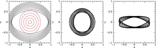
Left-hand panel: closed orbits; x1 orbits black and x2 orbits red. Centre and right-hand panels: an orbit that circulates inside the ILR and an orbit trapped by the ILR computed using resTorus_L. The potential has Bstrength = 0.1.
Each panel of Fig. 13 shows sections through tori associated with a rung of the ladder in the bottom panel of Fig. 9. As in Fig. 7, the blue dashed curves are sections through the axisymmetric tori that provide the basis for the perturbation theory. The red curves of each panel are sections through the tori returned by a single resTorus_L object for five values of the integral I. The black dots are consequents obtained by integrating the full equations of motion for |$147\, \mathrm{Gyr}$| from initial conditions provided by two of these tori. In contrast to Fig. 7, the dots do not lie on curves, indicating that the orbits are stochastic. The degree of stochasticity increases with the amplitude of libration. The boundaries of the region within which the consequents of an orbit scatter appear to be bounded by curves belonging to the family of red curves.
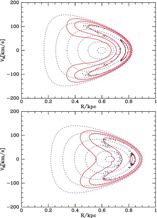
Surfaces of section for orbits trapped at the ILR. Red curves are computed from non-axisymmetric tori constructed using the axisymmetric tori whose cross-sections are plotted in dashed blue curves. Black points show consequents obtained by numerically integrating the full equations of motion from initial conditions given by one point on two of the red curves. The lower panel shows orbits on the lowest rung of the ladder in the bottom panel of Fig. 9, and the upper panel shows orbits on a higher rung.
6 RELATION TO REAL-SPACE PERTURBATION THEORY
Elementary treatments of perturbation of near-circular orbits by a non-axisymmetric component of the potential (e.g. Binney & Tremaine 2008, section 3.3.3) do not use angle-action coordinates. They proceed by perturbing Newton’s equations of motion to derive the equation of motion for the radial displacement ΔR of an orbiting star that is just the equation of motion of a driven harmonic oscillator. The particular integral of this equation corresponds to a closed orbit while the complementary function describes libration about this orbit. The orientation of the closed orbit provided by the particular integral switches through 90 deg across the resonance, but ΔR diverges as the resonance is approached. Sufficiently far from the resonance these solutions provide useful approximations to orbits such as those plotted in the right two panels of Fig. 12.
These solutions apply to the regime of low Jr in which there is no clear distinction between orbits that have or have not been trapped. Hence for angular momenta that are greater than that of the resonant orbit with Jr = 0, elementary theory provides an approximation that is valid until its amplitude ΔR becomes a significant fraction of R. For angular momenta smaller than that of the resonant orbit, the approximation is useful near the part (if any) of the Jϕ axis that lies below and to the left of the resonance’s ladder. The solutions do not describe orbits that lie within the ladder at values of |$J_3^{\prime }$| below the critical value at which trapping becomes sharply defined.
7 CONCLUSIONS
The algorithm used by tm to compute tori trapped at a Lindblad resonance has been improved so it can handle trapping at a Lindblad resonance of the least eccentric orbits. This step was necessary before tm could be used to investigate the impact of such resonances on the kinematics of the solar neighbourhood, which is the subject of a companion paper (Binney 2020). The key change is to switch from angle-action coordinates, which are polar coordinates for the slow plane, to Cartesian coordinates for the plane. This switch is only mandatory for orbits of low eccentricity, but it is expedient to make it for all orbits.
Orbits that are profoundly affected by a Lindblad resonance occupy an elongated volume of action space that slopes towards lower angular momentum Jϕ with increasing radial action, Jr. In this zone the vertical action Jz and a linear combination |$J_3^{\prime }$| of Jr and Jϕ is conserved to a good approximation, so orbits move along lines of constant |$(J_z,J_3^{\prime })$|. These lines constitute the rungs of a ladder. A new action |${\cal J}$| quantifies the magnitude of the excursions an orbit takes from the ladder’s centre line.
The higher rungs of the ladder have well-defined endpoints at which orbits cease to move to and fro across the ladder. We say that orbits that are located above or below the ladder circulate rather than librate.
A number of rungs near the bottom of the ladder reach the Jϕ axis. Consequently, at the corresponding values of |$J_3^{\prime }$| it is impossible to circulate inside the resonance. In contrast to rungs higher up the ladder, the lower rungs do not have well-defined upper ends at which libration suddenly gives way to circulation. Instead as the value of |${\cal J}$| increases, there is a continuous evolution of the orbit from libration around an orbit of a certain eccentricity that differs from an axisymmetric orbit only in that it does not precess, to motion that is qualitatively the same as that of an eccentric orbit in an axisymmetric potential.
Our numerical examples have used the potential defined by B18, which is a combination of a realistic axisymmetric Galaxy model and an analytic quadrupole. From the likely radius of corotation outwards this potential is barely differs from that fitted by S15 to the flow of gas through the Galactic disc. For this potential tm furnishes with ease tori for corotation and outwards that reproduce with precision the results of direct integration of the equations of motion.
At |$R\lesssim 3\, \mathrm{kpc}$| the potential’s quadrupole is smaller than that of S15, which is too strong to permit x2 orbits in the axisymmetric potential adopted by B18. In the vicinity of the ILR, both bars induce significant chaos in phase space, and are difficult to use in conjunction with tm because they require very eccentric tori. So our numerical examples of trapping at the ILR have been limited to a bar that has a tenth of the strength of the B18 bar. At this strength, there is limited chaos so one can study the structure of phase space cleanly.
In a companion paper, we use tm to understand better the orbits of stars that approach the Sun and may be trapped at either corotation or the OLR. It is currently unclear what scope tm has to assist in understanding phenomena deep inside the bar, where trapping by several resonances, especially the ILR, must be important. The indications are that orbits in this region are stochastic, but they are certainly not ergodic. So we have to find means to quantify them, and tm, or an upgrade of it, is a strong contender for this job. Given how profoundly orbits inside the bar differ from axisymmetric orbits, it is tempting to write code that produces triaxial tori directly rather than distorting axisymmetric images into triaxial tori by perturbation theory. On the other hand, surprisingly, the signs are that the limitations encountered here when applying tm inside the bar have less to do with the perturbation theory than with production of the underlying axisymmetric tori. In any event, the basic tm code requires further work, in particular to enable it to interpolate cleanly between tori when a point transformation is required.
ACKNOWLEDGEMENTS
I thank John Magorrian for an invaluable conversation. This work has been supported by the Leverhulme Trust and the UK Science and Technology Facilities Council under grant number ST/N000919/1.
Footnotes
By the reality of H1 we must always include also n = −N and Binney (2016) included also n = ±2N.
