


ABSTRACT
In the frame of the Solar system, the Doppler and aberration effects cause distortions in the form of mode couplings in the cosmic microwave background (CMB) temperature and polarization power spectra and, hence, impose biases on the statistics derived by the moving observer. We explore several aspects of such biases and pay close attention to their effects on CMB polarization, which, previously, have not been examined in detail. A potentially important bias that we introduce here is boost variance—an additional term in cosmic variance, induced by the observer’s motion. Although this additional term is negligible for whole-sky experiments, in partial-sky experiments it can reach 10 per cent (temperature) to 20 per cent (polarization) of the standard cosmic variance (σ). Furthermore, we investigate the significance of motion-induced power and parity asymmetries in TT, EE, and TE as well as potential biases induced in cosmological parameter estimation performed with whole-sky TTTEEE. Using Planck-like simulations, we find that our local motion induces |$\sim 1\!-\!2 {{\ \rm per\ cent}}$| hemispherical asymmetry in a wide range of angular scales in the CMB temperature and polarization power spectra; however, it does not imply any significant amount of parity asymmetry or shift in cosmological parameters. Finally, we examine the prospects of measuring the velocity of the Solar system w.r.t. the CMB with future experiments via the mode coupling induced by the Doppler and aberration effects. Using the CMB TT, EE, and TE power spectra up to ℓ = 4000, the Simons Observatory and CMB-S4 can make a dipole-independent measurement of our local velocity, respectively, at 8.5σ and 20σ.
1 INTRODUCTION
The motion of the Solar system with respect to the cosmic microwave background (CMB) creates mode couplings in the observed temperature and polarization anisotropies. These mode couplings can be interpreted as leakage of nearby harmonic multipoles into each other in the moving frame, inducing a scale-dependent change in the estimated power spectrum (Challinor & van Leeuwen 2002). The leakage is a result of the relativistic Doppler and aberration effects (Lorentz boost) caused by the motion of the observer (us) in the rest frame of the CMB. The largest component of this effect is the well-known CMB dipole moment – which is the rest-frame monopole leaking into the observed dipole in the moving frame (Kamionkowski & Loeb 1997; Yasini & Pierpaoli 2016; Yasini & Pierpaoli 2017a) – but the leakage exists among other multipoles as well. The mode coupling arising from the motion-induced leakage is usually disregarded, with the exception of the dipole, but it has been shown that depending on the geometry and sky/frequency coverage of the specific CMB experiment it can have non-trivial consequences and can potentially lead to biases in CMB statistics (Chluba 2011; Dai & Chluba 2014; Jeong et al. 2014; Yasini & Pierpaoli 2017b).
In the half portion of the sky towards the direction of motion, the primary effects of the boost on the power spectrum are (i) an overall increase in total power, and (ii) a decrease in the size of angular fluctuations1 (Yasini & Pierpaoli 2017b). The opposite holds in the antipodal half of the sky. These changes (i and ii) naturally lead to an asymmetry in the observed CMB power spectrum and any other statistics inferred from opposite halves of the sky. In this paper we examine several statistics that could be potentially affected by the boost, and assess the amount of motion-induced bias in them using realistic simulations.
In particular we look at (i) the impact of the Doppler and aberration effects on the CMB temperature and polarization power spectra and their corresponding cosmic variance, (ii) potential power and parity asymmetries induced in CMB maps as well as (iii) possible shifts in cosmological parameters in all-sky experiments. We also investigate (iv) prospects of future experiments for measuring our local velocity w.r.t. the CMB using motion-induced harmonic mode coupling. Some of these issues have been studied previously, but here we redo them using state-of-the-art theoretical modeling of the boost and include polarization and cross-spectra which are usually ignored.
We also introduce software that offers an accurate boosting formalism called COSMOBOOST,2 which employs the generalized Doppler and aberration kernel developed in Yasini & Pierpaoli (2017b) based on previous work by Dai & Chluba (2014). The calculations of the Doppler and aberration effect in this formalism are performed in harmonic space and hence the results are not prone to errors that incur in real-space boosting due to pixellization and finite window function (Yoho et al. 2013; Jeong et al. 2014). COSMOBOOST (Yasini 2019) also calculates the motion-induced spectral deviations of the CMB from blackbody in harmonic space (Yasini & Pierpaoli 2017b), which might also have an impact on deriving parameters from observations. However, these effects are expected to be small and would primarily impact other aspects of CMB data analysis (e.g. calibration) not considered here, and we therefore ignore them in this paper.
1.1 Boost variance
The motion of the observer changes the uncertainty associated with determining the underlying theoretical power spectrum from observations. We will show that in a naive analysis of the power spectrum, the boost changes the so-called cosmic variance; we call the resulting additional term boost variance and investigate its angular dependence and its relevance in different locations of the sky (see Section 3.3).
1.2 Power asymmetry
We will closely examine the effect of the Lorentz boost as a source of power asymmetry in the CMB (Dai et al. 2013; Aluri et al. 2015a,b; Das 2018; Shaikh et al. 2019) when observed in different portions of the sky, and in particular opposite hemispheres. This problem has been studied in Notari, Quartin & Catena (2014) and Quartin & Notari (2015) for CMB temperature; here we repeat the exercise using COSMOBOOST and include polarization spectra as well. Using simulations we show that Lorentz boost induces non-trivial (per cent level) hemispherical power asymmetry in TT, EE, and TE power spectra of a Planck-like experiment, and then compare the results with the observations from Planck (Akrami et al. 2019) (see Section 4).
1.3 Parity asymmetry
Aside from the well-known power asymmetry, the Planck maps deviate from the expected statistical isotropy through the so-called parity asymmetry, i.e. the odd multipoles carry more power than the even multipoles (Aluri & Jain 2012). Using simulations, we examine whether this could be caused by the motion of the observer (Naselsky et al. 2012) and investigate any potential parity asymmetry induced by the boost (see Section 5).
1.4 Cosmological parameter estimation
The motion-induced change in the power spectrum propagates to the inferred cosmological parameters as well. This issue has been reviewed in particular for the Planck parameter estimation in Catena & Notari (2013) using only the temperature power spectrum, a simplified treatment of the foreground mask, and a suboptimal boosting scheme. Here we revisit the problem but also include (i) polarization, (ii) the final Planck noise configuration and foreground mask, and (iii) the use of the accurate boosting formalism COSMOBOOST in simulating the power spectra (see Section 6). Furthermore, the effects on high ℓ(> 800) and low ℓ(< 800) modes are examined separately to investigate potential discrepancies induced in these two ranges for Planck. The outcome of the combination of various updates with respect to Catena & Notari (2013) is not immediately obvious – as some would lead to larger and others to smaller effects in parameter estimation. Therefore, it is worth redoing this exercise to ensure the Planck parameters are not biased by the Doppler and aberration effects.
1.5 Boost detection
It is possible to infer the direction and amplitude of our local bulk motion with respect to the CMB by measuring the coupling between the nearby multipoles. This effect was introduced in Kosowsky & Kahniashvili (2011) and Amendola et al. (2011) based on the original calculations by Challinor & van Leeuwen (2002), and later detected by Planck in Aghanim et al. (2014) using the CMB temperature. Since the amplitude of the coupling signal depends on the slope of fluctuation in the CMB angular power spectrum (see Section 7), it actually leaves a larger signature in polarization than in temperature.3 However, the polarization noise in Planck makes this component of the boost-coupling signal subdominant with respect to the one in temperature, and hence undetectable. The next generation of CMB surveys, however, will have lower noise levels, and will therefore measure the polarization power spectrum better, and extend the range of modes measurable in temperature. Although the upcoming experiments such as the Simons Observatory (SO) (Abitbol et al. 2019) and CMB-S4 (Abazajian et al. 2019a,b) are planned to observe a smaller fraction of the sky compared with Planck, their higher sensitivities will map the power spectrum with a greater precision at smaller scales, allowing for a better measurement of the motion-induced mode coupling. It is therefore worthwhile to exploit their enhanced capabilities to make a more accurate measurement of our local velocity, independent of the dipole component. Such measurements will be extremely valuable in lifting the degeneracy between the kinematic and intrinsic components of the CMB dipole (Roldan, Notari & Quartin 2016; Yasini & Pierpaoli 2017a). We will examine the prospects of this detection with SO and CMB-S4, and the synergy between these experiments and Planck.
1.6 Outline
The outline of this paper is as follows: Section 2 contains a summary of the notation and approximations used in this paper. In Section 3, we review the Doppler and aberration Kernel formalism and then investigate the effect of Lorentz boost on the CMB temperature and polarization harmonic multipoles and power spectra as well as their associated cosmic variance. In Section 4, we examine the hemispherical power asymmetry induced by the boost in both temperature and polarization spectra. Section 5 briefly inspects possible motion-induced parity asymmetries induced in CMB temperature and polarization power spectra. In Section 6, we examine the potential bias induced by the boost in cosmological parameter estimation for a Planck-like experiment. And, finally, in Section 7, the prospects of boost detection using large-sky CMB experiments such as SO and CMB-S4 are discussed. A summary of the results is presented in Section 8.
2 NOTATION AND APPROXIMATIONS
Throughout this paper, tilde |$(~\tilde{~})$| and prime (′) accents are reserved for variables and indices in the boosted frame. The explicit use of the prime notation repeatedly throughout the text is to remind the reader that the variables of analysis are evaluated in a boosted frame. Whenever necessary, the subscripts r and b are used to distinguish the rest and boosted frames w.r.t. the CMB. Unless noted otherwise, |$\Delta C_{\ell ^{\prime }} = \tilde{C}_{\ell ^{\prime }}-C_{\ell ^{\prime }}$| refers to the boosted minus rest-frame values of the estimated power spectrum. A primed index on a rest-frame observable such as |$C_{\ell ^{\prime }}$| means |$C_{\ell }|_{\ell =\ell ^{\prime }}$|. |$C^{XY}_\ell$| refers to the estimated power spectrum |$1/(2\ell +1)\sum a^{X*}_{\ell m}a^{Y}_{\ell m}$|, where X, Y ∈ {T, E}, and |${\boldsymbol {\mathbb {C}}}^{XX}_{\ell ^{\prime }}$| is used to indicate the underlying variance of the harmonic multipoles 〈|aℓ, m|2〉. The estimated power spectrum is typically expressed with a hat notation (|$\hat{C}_\ell$|); however, we chose this unconventional notation (simply Cℓ) for the estimator to avoid the use of two accents (tilde and hat) for the estimated power spectrum in the boosted frame. Whenever the word cosmic variance is accompanied by the symbol σ, it refers to the square root of 〈(Cℓ − 〈Cℓ〉)2〉.
The fiducial values for the cosmological parameters used in this paper ωb, ωc, θ, As, ns, H0, and σ8 are, respectively, 0.022, 0.119, 1.042, 2.3 × 10⁻⁹, 0.9667, 67.74, and 0.860. We also fix reionization τ = 0.066 to avoid complications in dealing with small ℓ values in parameter estimation. The values of cosmological parameters used are not the ones preferred by the most updated Planck 2018 results (Aghanim et al. 2018); however, since here we are concerned only with the amount of shift in these parameters induced by the boost, their actual values are of little importance in this study. Finally, h, k, and c refer to the Planck, Boltzmann, and speed of light in vacuum constants, respectively.
We use the Planck 143-GHz mask4 as the primary mask in the study. The 100- and 217-GHz masks have, respectively, smaller and larger areas covered with respect to the 143-GHz mask. This means that we should expect the boost effects in the power spectrum to be slightly weaker for the former and stronger for the latter (Pereira et al. 2010). For this reason, we chose to use the 143-GHz mask to get a reasonable estimate of the effect in the combined maps.
In the calculations of the aberration kernel and its analytical estimates, we do not account for the frequency dependence of the boost because it is negligible for the cases studied here (especially for experiments with relatively symmetric masks such as Planck). These effects can become non-trivial for partial-sky surveys though and should be taken into account. Additionally, we neglect any effects due to extragalactic foregrounds (Chluba, Hütsi & Sunyaev 2005; Balashev et al. 2015). Also, for simplicity, we do not consider the CMB B-mode power spectrum throughout this paper (see Yasini & Pierpaoli 2017b for details on motion-induced E to B leakage).
3 THE EFFECT OF OUR MOTION ON TEMPERATURE AND POLARIZATION STATISTICS
3.1 Doppler and aberration kernel formalism
Fig. 1 shows the shape of the kernel |$_{T}\mathcal {K}^m_{{\ell ^{\prime }}{\ell ^{\prime }+\Delta \ell ^{\prime }}}$| for a few different multipoles ℓ′, and a range of −8 < Δℓ′ < 8. Each point represents the amount of motion-induced leakage from multipole ℓ′ + Δℓ′ into the observed ℓ′ mode. In the moving frame, a multipole ℓ′ observed in the hemisphere towards the direction of motion leaks into its higher neighbours (ℓ′ + 1, ℓ′ + 2, etc.) and receives a contribution from its lower neighbours (ℓ′ − 1, ℓ′ − 2, etc.). And the opposite happens in the other hemisphere. With this in mind, one can interpret the Δℓ′ < 0 (Δℓ′ > 0) terms in the kernel as the contribution of modes towards (away from) the direction of motion.
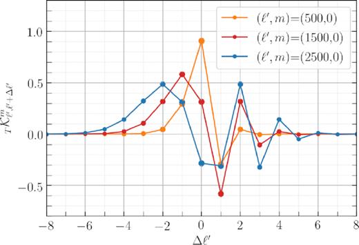
The general behaviour of the Doppler and aberration kernel for thermodynamic temperature T. The kernel coefficient |$_{T}\mathcal {K}^m_{{\ell ^{\prime }}{\ell }}$| denotes the amount of motion-induced leakage from the spherical harmonic coefficient aℓm in the rest frame, into the observed |$a_{\ell ^{\prime } m}$|. The y-axis shows the leakage components from a range of −8 < Δℓ′ < 8 neighbours into observed modes ℓ′ =500, 1500, and 2500 at m = 0. As we increase ℓ′, the kernel becomes more non-linear and the contribution from farther neighbours becomes more important and, hence, non-negligible. The kernel coefficients generally become smaller as m → ℓ′. Also, at ℓ′ ≫ 2 the polarization kernel |$_{E}\mathcal {K}^m_{{\ell ^{\prime }}{\ell }}$| converges to |$_{T}\mathcal {K}^m_{{\ell ^{\prime }}{\ell }}$|.
At low ℓ′ the kernel starts very linearly (≈βℓ′) with a sharp peak at Δℓ′ = 0 (Challinor & van Leeuwen 2002). But as we pass ℓ′ ≳ 1/β ≈ 800, the behaviour of the kernel becomes non-linear (deviates from the βℓ′ approximation), and the central element Δℓ′ = 0 does not have the highest value anymore (Chluba 2011). In other words, at this range, the leakage from farther neighbours becomes far greater than one would naively expect. For the high values of ℓ′ presented in the plot, the kernel for polarization is practically the same; the difference between the temperature and polarization kernel coefficients is of the order of ∼1/(ℓ2 − 2).
3.2 Boosted power spectrum
3.2.1 Analytical estimate
3.2.2 Simulations
Using the formalism presented in the previous subsection, we now examine the amount of motion-induced distortion in the CMB power spectra using 100 rest-frame and boosted simulations. In order to gauge the significance of the effect in the observed CMB sky, we follow the example in Jeong et al. (2014) and split the Northern hemisphere into five equal-area strips (assuming the observer is moving towards |$\hat{\boldsymbol z}$|). Then, we look at the relative difference between the rest-frame and boosted-frame power spectra in each of these strips for an individual simulation, as well as the average of the ensemble.
Fig. 2 shows the motion-induced fractional change |$\Delta C_{\ell ^{\prime }}/C_{\ell ^{\prime }}$| in five equal-area bands in the Northern hemisphere for TT and EE power spectra. There are obvious general characteristics in the plot that are expected for the ensemble average of the boost according to equation (8): (i) The effect is more prominent in the strips closer to the North Galactic Pole because the Doppler and aberration effects are stronger in directions closer to the apex of motion. (ii) In the Northern hemisphere, there is an overall increase in the power that becomes larger as we get to smaller angular scales (higher ℓ modes) – this is a direct consequence of the fact that the aberration effect changes the relative size of smaller anisotropies more strongly than it does for large scales.5 (iii) Since the amount of power leakage depends on the slope of the power spectrum, the relative changes in TT and EE fluctuate out of phase with respect to the corresponding rest-frame spectra (second term in equation 8). By the same token, since the EE has more pronounced fluctuations than the TT power spectrum, the relative change is in general larger in polarization than in temperature. As we will discuss in more detail in Section 7, for an experiment with low instrumental noise, this very fact makes the detection of the boost – using mode coupling – easier in polarization than in temperature (see Appendix B for the TE power spectrum plots). It is also worth noting that although the behaviour of the kernel becomes non-linear in β for ℓ ≳ 1/β ≃ 800, equation (8) still performs very well in approximating the ensemble average of the boosted power spectra in this range.
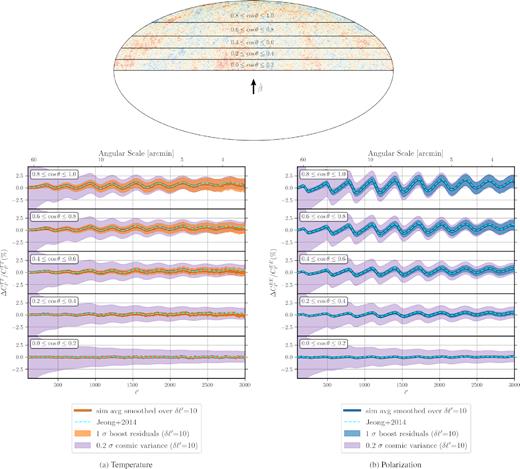
Induced relative change in the CMB power spectra (|$\Delta C_{\ell ^{\prime }}/C_{\ell ^{\prime }} = \tilde{C}_{\ell ^{\prime }}/ C_{\ell ^{\prime }} -1$|) due do the Doppler and aberration effects induced in a frame moving towards the Northern Galactic Pole. Individual plots, respectively, show this change for TT (left-hand panel) and EE (right-hand panel), in five equal-area strips in the Northern hemisphere (top panel). The thick solid lines (orange for TT and blue for EE) show the average of 100 simulations Gaussian smoothed over a δℓ′ = 10 scale. The effect becomes larger towards the direction of motion (highest panels in both plots) and in general is more prominent in EE than in TT. The analytical formula from Jeong et al. (2014) (dashed cyan) emulates the average effect extremely well, but if used for correcting individual power spectra, it leaves residuals in the data. The shaded bands (orange for TT and blue for EE) around the simulation average show the 1σ region for the boost residuals left in individual realizations of the power spectrum, which can be as large as 20 per cent of cosmic variance (purple band) at ℓ ≃ 3000 for both TT and EE (see equation 10).
An important point that might not be immediately obvious from Fig. 2 is that the oscillating patterns emerge in the Southern hemisphere with the opposite sign (cos θ → −cos θ: ΔCℓ/Cℓ → −ΔCℓ/Cℓ in |$\mathcal {O}(\beta$|)). The crucial consequence of this statement is that when one calculates the power spectrum over a patch of the sky that is symmetric w.r.t. cos θ, the motion-induced effects cancel each other to first order in β. As we will show in Section 6, this is roughly the case for Planck, which has a mask that is fairly symmetric w.r.t. the peculiar velocity unit vector |$\hat{\boldsymbol \beta }$| (also see section IV.B in Jeong et al. 2014).
3.3 Boost variance
3.3.1 Analytical estimate
Aside from inducing a shift in the statistical average of the power spectrum at every ℓ, the Doppler and aberration effects also change the variance of each mode. In what follows, we will quantify this variance analytically. For simplicity, we drop the XX superscript from all |$C^{XX}_\ell$| and |${\boldsymbol {\mathbb {C}}}^{XX}_\ell$|, and the prime (′) accent in this subsection.
The motion of the observer increases the variance of the ensemble of observed power spectra both towards (|$\overline{\cos \theta }\gt 0$|) and away from (|$\overline{\cos \theta }\lt 0$|) the direction of motion, and has a minimal effect on the motion’s equatorial plane (|$\overline{\cos \theta }\simeq 0$|). In a partial sky experiment, the sample variance can be easily calculated from this expression via |$\tilde{\sigma }^2_\ell /f_{\rm sky}$|, where fsky is the fraction of sky covered by the survey (Scott, Srednicki & White 1994).
3.3.2 Simulations
Fig. 3 shows the significance of boost variance for the five equal-area cuts of Fig. 2. Here the left- and right-hand plots show the relative motion-induced change in the standard deviation |$\Delta \sigma ^{XX}_\ell /\langle C^{XX}_\ell \rangle = (\tilde{\sigma }^{XX}_\ell - \sigma ^{XX}_\ell)/\langle C^{XX}_\ell \rangle$| for temperature (X = T) and polarization (X = E), respectively. As expected, the change due to boost variance is larger towards the direction of motion (higher panels) and smaller angular scales (higher ℓ), and the effect is generally larger in polarization than in temperature. In the topmost panel, which represents |$f_{\rm {sky}}=10{{\ \rm per\ cent}}$| of the sky towards |$\hat{\boldsymbol \beta }$|, the effect is around 10 per cent of rest-frame cosmic variance (σℓ) in TT and 20 per cent in EE.
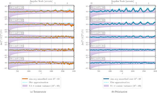
Boost variance (shift in the cosmic variance due to the Doppler and aberration effects) in the five equal-area strips of Fig. 2, normalized by the rest-frame power spectrum. Individual plots, respectively, show this change for TT (left-hand) and EE (right-hand) spectra. The solid lines (orange for TT and blue for EE) show the average difference between cosmic variance in the boosted frame |$\tilde{\sigma }_\ell$| (equation 13) and rest frame σℓ (equation 12) for 100 simulations Gaussian smoothed over a δℓ′ = 10 scale. The increase due to the boost variance can be as large as 10 per cent of rest-frame cosmic variance (purple band) for TT, and 20 per cent for EE at ℓ ≃ 3000. Similar to what happens to the average of the power spectrum shown in the previous plot, the variance also becomes larger towards the direction of motion (higher panels in both plots) and in general is more prominent in EE than in TT. Unlike the average, however, the variance does not change the sign in the Southern hemisphere (not shown here). Our analytical formula in equation (13) approximates the effect closely, but slightly overestimates it at its peaks.
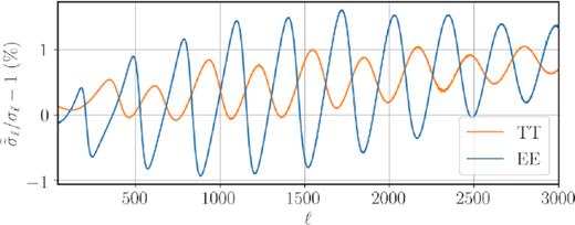
Relative change in cosmic variance due to the boost after correcting the mean power spectrum |${\boldsymbol {\mathbb {C}}}_\ell \rightarrow \tilde{{\boldsymbol {\mathbb {C}}}}_\ell$|.
The motion-induced effects in the power spectrum change the mean and variance of the inferred cosmological parameters. Here we estimate the change in the variance using the Fisher matrix. By propagating the variance in equation (14) to inferred cosmological parameters via the Fisher matrix |${{\sf F}}_{ij}=\sum _\ell \tilde{{\boldsymbol {\mathbb {C}}}}_\ell ^{-2} \partial _i\tilde{{\boldsymbol {\mathbb {C}}}}_\ell \partial _j\tilde{{\boldsymbol {\mathbb {C}}}}_\ell$| (Tegmark 1997) up to ℓmax = 5000, we found that the error bars on all parameters are affected at most by 0.015σ in both TT and EE, assuming |$\overline{\cos \theta }=1$|; this includes only the change in variance and not the shift in parameters, which can be an order of magnitude larger. Therefore, correcting the boost in the average (or theoretical) power spectrum should sufficiently remove any bias propagated to the inferred parameters from |$\tilde{C}_\ell$|.
3.4 Accounting for the boost: practical guide
After the theoretical insights of the previous sections, it is sensible to ask what is the best strategy to correct for the boost in using the CMB to derive cosmological parameters. Here is a summary of possible deboosting methods:
Real space deboosting, The Doppler and aberration effects can be corrected at the map level on individual pixels. This approach potentially underestimates the boost effect at small angular scales, and is sensitive to the pixel window function (Yoho et al. 2013).
Harmonic space deboosting. The spherical harmonic coefficients aℓm can be deboosted with the Doppler and aberration kernel formalism of COSMOBOOST. This is the most accurate way to deboost the CMB without leaving any residuals in the average or variance of Cℓ (Yasini & Pierpaoli 2017b).
Corrections to the power spectrum. Equation (8) (Jeong et al. 2014) provides an excellent estimate for the effect of the boost on the theoretical power spectrum |${\boldsymbol {\mathbb {C}}}_\ell$|. If the analysis demands a comparison between the observed (boosted) power spectrum |$\tilde{C}_{\ell ^{\prime }}$| and the theoretical |${\boldsymbol {\mathbb {C}}}_\ell$| – e.g. likelihood analysis in parameter estimation – there are two ways this equation can be used to correct for the boost: (i) boost the theoretical power spectrum for a given model |${\boldsymbol {\mathbb {C}}}_\ell \rightarrow \tilde{{\boldsymbol {\mathbb {C}}}}_\ell$| directly, and (ii) use the ensemble average |$\tilde{{\boldsymbol {\mathbb {C}}}}_{\ell ^{\prime }}$| to deboost the observed power spectrum |$\tilde{C}_{\ell ^{\prime }}$|. In both cases, the correct variance to use is represented by equation (14).
Note: If no boost correction is performed on the observed |$\tilde{C}_{\ell ^{\prime }}$| at all, the average and variance are biased, respectively, by equations (8) and (13).
Assuming the amplitude and direction of the boost are known, the most accurate way to deboost an observed map is to use COSMOBOOST. In this approach, the individual spherical harmonic coefficients are deboosted and no residuals are left neither in the map nor in the estimated power spectrum. Moreover, the final product can be reliably used in cross-correlation analysis. The downside is that calculating and storing the kernel coefficients can become numerically prohibitive at very high ℓ.
Alternatively, if one is interested only in the power spectrum Cℓ (and not the map or aℓm), one can use the Jeong et al. (2014) formula to correct for the boost effects. In such a case, it is advisable to apply equation (8) to the theoretical (rest-frame) power spectrum for a given set of parameters before comparing to the data. The variance in this case is given by equation (14).
Which experiments should care to explicitly correct for the boost? The CMB power spectrum of whole-sky and/or symmetric-sky experiments (e.g. Planck and SO) will not be impacted by the boost: The dependence of the observed spectrum on |$\overline{\cos \theta }$| ensures that the corrections are negligible (|$\overline{\cos \theta }\simeq 0$|). However, should a smaller area of the experiment be used in cross-correlation analysis with other types of surveys, it might be appropriate to deboost, given the effect of the boosting on individual ℓ modes (see Fig. 2).
In partial-sky experiments, the effects of the boost should be evaluated on the basis of where the area observed is located on the sky, as well as the attainable precision in cosmological parameter estimation (also influenced by instrumental characteristics like beam size and noise level). If no boost correction is applied (e.g. BICEP, POLARBEAR), the average and variance of the power spectrum are biased according to equations (8) and (13), which can be used to assess the approximation made.
Other experiments have used the Jeong et al. (2014) formula to try and correct for the Doppler and aberration effects. ACTPol (Louis et al. 2017) uses the boosted ensemble average |$\tilde{{\boldsymbol {\mathbb {C}}}}_\ell$| to subtract the average effect from the observed power spectrum |$\tilde{C}_{\ell ^{\prime }}$|. SPTPol (Henning et al. 2018) opted for the strategy of boosting the theoretical |${{\boldsymbol {\mathbb {C}}}}_{\ell }$| before comparing it with the observational points in the likelihood analysis. In both these cases, the standard (rest-frame) cosmic variance should be replaced with equation (14). In general, if a map-level correction with COSMOBOOST is not feasible, the latter approach is recommended since it introduces a minimal error due to leftover boost effects (Section 3.2).
4 HEMISPHERICAL POWER ASYMMETRY IN THE POWER SPECTRUM
Since the Doppler effect increases the brightness of the incoming radiation on all angular scales in the direction of motion – and decreases it on the opposite side – it creates a power asymmetry in the two hemispheres. It was discovered in Eriksen et al. (2004) that the WMAP power spectrum calculated over different patches of the sky does not seem to be statistically isotropic. This anomaly was later confirmed in the Planck maps as well (Planck Collaboration XXIII 2014; Planck Collaboration XVI 2016; Akrami et al. 2019). It is worth looking into how the motion of the observer affects the power distribution in the CMB, and possibly shed light on the hemispherical asymmetry anomaly observed in the CMB map. This exercise has been performed for the CMB temperature in Notari et al. (2014) and Quartin & Notari (2015), but here we repeat it using the accurate formalism of COSMOBOOST, and also include polarization [see Mukherjee, De & Souradeep (2014) for an analytical examination using bipolar spherical harmonics (Hajian & Souradeep 2003)].
As discussed in the previous section, the observed power spectrum increases in the direction of motion proportional to |$\beta \ell ^{\prime } \overline{\cos \theta ^{\prime }} \textrm{{d}}C_{\ell ^{\prime }}/\textrm{{d}}\ell ^{\prime }$| (see Fig. 2). Since |$\overline{\cos \theta ^{\prime }}$| is positive in the Northern hemisphere and negative in the Southern hemisphere, this naturally leads to a power asymmetry in the observed CMB anisotropies both in temperature and polarization. In order to gauge the amount of motion-induced asymmetry in the CMB sky, we take the following steps: We split the Planck foreground mask into the Northern and Southern hemispheres, then rotate them to the |$\hat{\boldsymbol \beta } \rightarrow \hat{\boldsymbol z}$| frame. We then apply these masks to 100 rest-frame and boosted simulations. We then calculate the power spectra of all maps and look at the relative difference between the boosted and rest-frame results in each hemisphere.
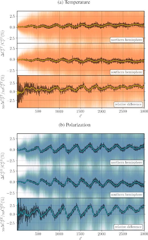
Motion-induced hemispherical asymmetry for a Planck-like experiment in (a) temperature and (b) E-mode polarization. The faint lines in the background (orange for TT and blue for EE) are 100 individual simulations plotted on top of each other to show the overall variance of the effect. The dark jagged lines are the average of the 100 simulations in all panels. The coloured smooth lines are the average of simulations Gaussian smoothed over the scale of δℓ′ = 10. As evident from the bottom panels of each plot, Doppler and aberration effects induce a per cent level power asymmetry between the hemispheres, which is more accentuated in EE. See equation (16) in the text for the definition of the statistics presented in the bottom panels.
Now, let us evaluate this statistic on the Planck temperature and polarization data. Fig. 6 shows the relative difference in power between the Northern and Southern hemispheres of the Planck SMICA map in comparison with simulations. As evident from the plot, although the hemispherical asymmetry of the SMICA power spectra has the expected sign as the ones induced by the local motion, it is unlikely that the entire deviation is explained by the Doppler and aberration effects. Nevertheless, the oscillations in the north–south power asymmetry of Planck SMICA over various angular scales – especially in the case of TT up to ℓ′ ≲ 1500 – marginally follow the same frequency as the motion-induced oscillations in the simulations, which suggests that these patterns are at least in part induced by the boost. A key point here is that since the Planck maps have not been corrected for the Doppler and aberration effects, we know that their footprints inevitably exist in the observational data. However, an accurate determination of exactly how much of the effects shown here is due to Doppler and aberration and how much due to foregrounds, mask, and other systematic contaminations requires a more rigorous examination. Here we merely point out the similarity between the motion-induced pattern in observation and simulations, but we avoid overinterpretation of this partial correspondence between the two, and postpone a detailed analysis to future work. A similar plot for the TE power spectrum is presented in Fig. B4.
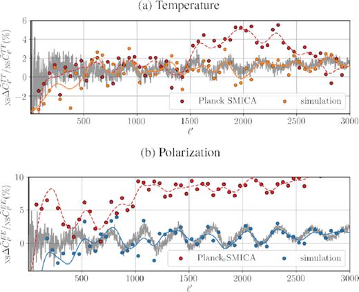
Relative difference between the Northern and Southern hemisphere power spectra in (a) temperature (top panel) and (b) E-mode polarization (bottom panel) of the Planck SMICA map binned (red circles) and also Gaussian smoothed (red dashed lines) by δℓ′ = 50. The average of 100 simulations (grey lines) are shown here for comparison, as well as an individual simulation binned (orange and blue circles) and Gaussian smoothed (orange and blue lines). The Gaussian-smoothed lines for Planck and simulations are provided for easier visual tracking of the general features of the power asymmetry. The oscillations in north–south difference in power spectra of Planck SMICA marginally follow the ones induced by the boost in simulations, suggesting that they might be partially due to the Doppler and aberration leftovers in the map. See equation (16) in the text for the definition of the statistics used in the plots.
5 PARITY ASYMMETRY
Fig. 7 shows the average of the parity statistic RXX for 100 simulations in the rest frame and boosted frame, with the shaded areas indicating the 1σ regions (standard deviation of the rest-frame simulations). The top and bottom plots, respectively, present RTT and REE. The top panel shows the RTT of the Planck SMICA map (dotted red), which is about 2σ away from the simulation average. The average amount of parity asymmetry induced in the simulations up to ℓmax = 500 (range shown in the plot) is only about 0.05σ for TT and 0.03σ for EE. Therefore, it can be safely concluded that since our local motion does not generate any significant parity asymmetry, it is not the relevant source of this observed anomaly in the CMB. Repeating this exercise only for the Northern hemisphere (Southern hemisphere masked) results in RTT = 0.04σ and REE = 0.06σ, so it is unlikely that the results will be significantly different in masked skies.
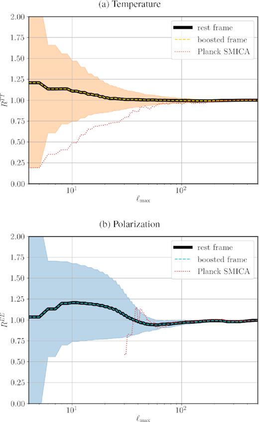
Motion-induced parity asymmetry for a Planck-like experiment in (a) temperature (top panel) and (b) E-mode polarization (bottom panel). The parity asymmetries in the rest frame (thick solid) and boosted frame (dashed) are almost identical. The shaded regions show the 1σ standard deviation of 100 simulations. The 1σ region for the boosted frame is almost identical to that of the rest frame as well and is not shown in the plot. The parity asymmetry in the Planck SMICA map (dotted) is shown for comparison. See equation (17) in the text for the definition of the statistics presented in the plot.
6 PARAMETER ESTIMATION WITH PLANCK POWER SPECTRUM
In this section, we investigate how much the motion of the Solar system changes the cosmological parameters inferred from the CMB power spectrum, as measured by Planck. As shown in Section 4, our local motion changes the power spectrum up to ∼2 per cent in each hemisphere. However, since Planck’s observation patch is relatively symmetric w.r.t. |$\hat{\boldsymbol \beta }$|, the effects we observe in the Northern hemisphere (contracted angular scales of anisotropies and enhanced amplitudes) get cancelled out by the opposite effects in the Southern hemisphere (expanded angular scales and diminished amplitudes) when calculating the power spectrum on the whole sky.
Fig. 8 shows the effect of the boost on the whole-sky temperature and polarization power spectra. A comparison with Fig. 5 reveals how the effects in the Northern and Southern hemispheres have cancelled each other, reducing the effect to only |$\mathcal {O}(\beta ^2)$| (Challinor & van Leeuwen 2002; Burles & Rappaport 2013). The average change in power spectra reduces to 0.05 per cent for both TT and EE.7 Note that similar to the half-sky case, despite the small shift in the average (or Gaussian smoothed) effect, the changes in individual modes of Cℓ are still much larger and can reach a few per cent. In order to emphasize this fact, we have kept an individual simulation in the plot binned by δℓ′ = 10 (the fluctuations on individual ℓ′ modes exceed 1 per cent and are not shown in the plot). The main question here is how much of the change in an individual Cℓ realization propagates to the inferred cosmological parameters in a Planck-like experiment.
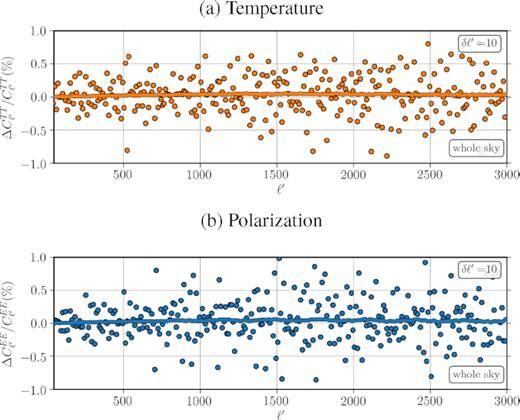
Relative change in the power spectrum of a whole-sky map for (a) temperature (top panel) and (b) E-mode polarization (bottom panel). The average of 100 simulations is Gaussian smoothed with δℓ′ = 10 (solid line). A random simulation is chosen as representative of the sample, then binned with δℓ′ = 10 (circles) in both plots. The overall change in the ensemble average is only about 0.05 per cent in both plots, but the binned residuals around the average can be as large as 1 per cent.
In order to assess the relevance of the motion-induced bias for cosmological parameter estimation, we run maximum-likelihood analysis on simulated CMB temperature and polarization maps corresponding to the {100, 143, 217} (GHz) channels of Planck with the noise configuration {77.4, 33.0, 46.8} (μK-arcmin) for temperature and {117.6, 70.2, 105.0} (μK-arcmin) for polarization and {10.0, 7.3, 5.0} (arcmin) beam (Akrami et al. 2018). We take the following steps to prepare the data set for the analysis:
Calculate the TT, EE, and TE theoretical CMB power spectra using the five fiducial parameters (ωb, ωc, θ, As, ns) (see Section 1) with CAMB8 (Lewis, Challinor & Lasenby 2000).
Simulate temperature and polarization CMB maps from the theoretical Cℓ using healpy.synfast up to lmax = 3000 and NSIDE = 1024.
Boost a copy of the simulated map using the COSMOBOOST code. This map represents what would be observed in a frame moving with the velocity β = 0.001 23 in the |$\hat{\boldsymbol {z}}$|-direction.
Apply the Planck foreground mask to both maps. Since the Doppler and aberration kernel formalism boosts the map in the |$\hat{\boldsymbol \beta }= \hat{\boldsymbol z}$| direction, we rotate the mask to the same coordinate system. The output of this step is a CMB map observed in a frame moving with β = 0.001 23 in the |$\hat{\boldsymbol \beta }= (268^\circ , 48^\circ)$| direction.
Calculate the power spectrum of both rest-frame and boosted maps using pymaster9 (Alonso, Sanchez & Slosar 2019) to correct for the coupling among nearby multipoles induced by the mask.
Binning the power spectrum in general reduces the effect of the boost on the change in the power spectrum. Here we do not consider a binning scheme so that we can gauge the maximum possible effect; we use the power spectra with |$\delta \ell ^{\prime }_{\rm bin}=1$|.
Using the two power spectra obtained from the preparation steps – one in the rest frame and the other in the boosted frame – we perform a maximum-likelihood parameter estimation with the Markov chain Monte Carlo code monte-python 3 (Brinckmann & Lesgourgues 2018). For simplicity, instrumental noise is directly added to the power spectra, not at the map level. We employ the likelihood of Hamimeche & Lewis (2008) for two different configurations in TTTEEE : (i) whole range of angular scales probed by Planck (2 ≤ ℓ ≤ 2500), and (ii) high ℓ (2 ≤ ℓ ≤ 800) versus low ℓ (801 ≤ ℓ ≤ 2500).
Fig. 9 shows the results of parameter estimation using TTTEEE spectra in the range 2 ≤ ℓ ≤ 2500 from one random simulation, both in the rest frame (red) and in the boosted frame (dotted black). The contour lines of both frames almost overlap, demonstrating the almost perfect cancellation of the boost effect in the Northern and Southern hemispheres. To ensure this cancellation is not merely due to a chance in the particular simulation we analysed, we repeat the exercise with nine more realizations of the power spectra and look at the average shift in the parameters due to boost and compare this with the error bars on each parameter.
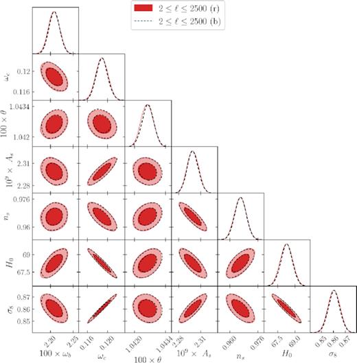
Parameter constraints from rest-frame and boosted-frame TT, EE, and TE spectra in the range 2 < ℓ < 2500 for a Planck-like experiment. The contour lines are 68 per cent and 95 per cent confidence intervals. The shift in parameters is only of the order of 0.02σ, which is why the rest-frame (r) and boosted-frame (b) contour lines overlap. Here the reionization optical depth τ is fixed to avoid complications in the low-ℓ parameter estimation. See Table 1 for the average shift in parameters due to the boost.
Table 1 shows the result of this analysis for all 10 simulations. The average shift in the parameters is on average about 0.02σ, with sound horizon θ being the most affected (∼0.06σ) and curvature perturbation amplitude As being the least affected (∼0.01σ). The errors on the numbers reported in the last column of the table are less than 20 per cent, so we decided that 10 simulations suffice for this analysis.
The average mean and standard deviation of 10 parameter estimations from boosted- and rest-frame simulations. μr and μb are the average of the inferred parameters in the rest and boosted frames. σr is the average variance of each corresponding parameter in the rest frame. The last column reports the shift in the mean of parameters due to Doppler and aberration effects, normalized by the intrinsic error in each parameter.
| Parameter | μr | σr | μb | 2 < ℓ < 2500 |
|---|---|---|---|---|
| |μb − μr|/σr | ||||
| 100 × ωb | 2.199 840 | 0.010 810 | 2.199 801 | 0.033 |
| ωc | 0.118 559 | 0.001 181 | 0.118 573 | 0.021 |
| 100 × θ | 1.042 673 | 0.000 156 | 1.042 689 | 0.059 |
| 109 × As | 2.298 937 | 0.006 144 | 2.298 919 | 0.012 |
| ns | 0.966 851 | 0.002 069 | 0.966 827 | 0.023 |
| H0 | 68.345 63 | 0.527 770 | 68.345 44 | 0.021 |
| σ8 | 0.860 056 | 0.005 154 | 0.860 113 | 0.021 |
The average motion-induced shift in the mean of estimated parameters in the rest frame (μr) and boosted frame (μb), normalized by the rest-frame uncertainty in each parameter (σr). The results are overall larger than the ones obtained from the whole range of 2 < ℓ < 2500 in Table 1.
| Parameter | 2 ≤ ℓ ≤ 800 | 801 ≤ ℓ ≤ 2500 |
|---|---|---|
| |μb − μr|/σr | |μb − μr|/σr | |
| 100 × ωb | 0.042 | 0.029 |
| ωc | 0.034 | 0.047 |
| 100 × θ | 0.073 | 0.057 |
| 109 × As | 0.033 | 0.060 |
| ns | 0.056 | 0.059 |
| H0 | 0.034 | 0.044 |
| σ8 | 0.030 | 0.044 |
| Parameter | 2 ≤ ℓ ≤ 800 | 801 ≤ ℓ ≤ 2500 |
|---|---|---|
| |μb − μr|/σr | |μb − μr|/σr | |
| 100 × ωb | 0.042 | 0.029 |
| ωc | 0.034 | 0.047 |
| 100 × θ | 0.073 | 0.057 |
| 109 × As | 0.033 | 0.060 |
| ns | 0.056 | 0.059 |
| H0 | 0.034 | 0.044 |
| σ8 | 0.030 | 0.044 |
The results that we find on the shift of parameters are typically smaller than the ones reported by Catena & Notari (2013), which considers only temperature. This is likely due to the fact that their boosting formalism slightly overestimates the effect (see fig. 2 in Dai & Chluba 2014). Inclusion of polarization information (EE, TE) does not affect the average shift in parameters significantly compared to chains that run only with the TT power spectrum. The EE-only runs also yield similarly negligible shifts in parameters.
Fig. 10 shows similar results for the TTTEEE parameter estimation but with 2 ≤ ℓ ≤ 800 and 801 ≤ ℓ ≤ 2500 plotted separately. In the 2 ≤ ℓ ≤ 800 regime, θ is still the most affected parameter – understandably so, because it is primarily determined by the position of the first peak. However, in the range 801 ≤ ℓ ≤ 2500, the two parameters As and ns are also affected comparably. Overall, the shift in parameters is still negligible and remains smaller than 0.1σ for all of them. In this analysis, we did not consider the frequency dependence of the boost effect, which is negligible for experiments with symmetric (w.r.t. the direction of motion) masks such as Planck (Yasini & Pierpaoli 2016). This effect could be potentially important for partial-sky experiments, but we postpone a detailed analysis of its implications for cosmology to future studies.
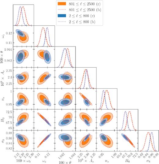
Parameter constraints from rest-frame and boosted-frame TT, EE, and TE spectra in the ranges 2 < ℓ < 800 (blue) and 801 < ℓ < 2500 (orange). The contour lines are 68 per cent and 95 per cent confidence intervals. The shift in parameters is slightly larger than the ones in Fig. 9, but still negligible (see Table 2).
7 BOOST DETECTION USING HARMONIC MODE COUPLING
The amount of motion-induced leakage of the nearby multipoles into each other depends on the amplitude and direction of the local peculiar velocity vector with respect to the CMB rest frame. Therefore, measurements of this induced-mode coupling in CMB temperature and polarization – which have well-known statistics – can be exploited to measure the local peculiar velocity vector. This idea has been investigated in detail in Kosowsky & Kahniashvili (2011), Amendola et al. (2011), and Notari & Quartin (2012), and the signal has been detected by Planck using 500 < ℓ < 2000 of 143- and 217-GHz channel maps (Aghanim et al. 2014) reporting a value of |$\beta =0.00128 \pm 0.00026\,(\rm {stat.})\pm 0.00038\,(\rm {syst.})$|. Here we present estimates for the achievable signal-to-noise ratio (S/N) with future surveys such as SO and CMB-S4, and compare their performance with Planck.
Sensitivity and beam configuration used for Planck, SO, and CMB-S4.
| Temperature | Polarization | Beam | |
|---|---|---|---|
| (μK-arcmin) | (μK-arcmin) | (arcmin) | |
| Planck (143 GHz) | 33 | 70 | 7.3 |
| Planck (217 GHz) | 47 | 105 | 5.0 |
| SO (145 GHz) | 10 | 14 | 1.4 |
| SO (225 GHz) | 22 | 31 | 1.0 |
| CMB-S4 nominal | 1 | 1.4 | 1.4 |
| Temperature | Polarization | Beam | |
|---|---|---|---|
| (μK-arcmin) | (μK-arcmin) | (arcmin) | |
| Planck (143 GHz) | 33 | 70 | 7.3 |
| Planck (217 GHz) | 47 | 105 | 5.0 |
| SO (145 GHz) | 10 | 14 | 1.4 |
| SO (225 GHz) | 22 | 31 | 1.0 |
| CMB-S4 nominal | 1 | 1.4 | 1.4 |
Fig. 11 shows the estimated S/N from Planck (left-hand panel), SO (middle pnael), and CMB-S4 (right-hand paanel). Each plot shows the S/N in TT (dashed), EE (dotted), and TE (dot–dashed) separately, and all combined (solid). Planck clearly becomes noise dominated at ℓ > 2000, and it can obtain only an S/N of about 4.5 with a minimal contribution from EE and TE. SO, despite its smaller sky fraction and, hence, coverage of a lower number of m modes for a given ℓ, has a much lower instrumental noise and can supersede Planck in the detection of this signal. Using only EE, SO can achieve a similar S/N to Planck (compare the dotted line in the middle panel to the solid line in the left-hand panel). Combining TT, EE, and TE for SO results in a total S/N of 8.5, roughly twice as large as Planck’s. Notice that below ℓ ∼ 2000, where the SO EE is not noise limited, it gains a large S/N compared to TT (compare dotted and dashed lines in the middle panel). As pointed out before, since the EE power spectrum fluctuates more abruptly than TT, it yields a larger mode coupling in the boosted frame. Finally, for comparison, we also show the results for CMB-S4, which can attain a total S/N of around 20.
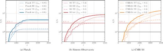
Boost detection (via mode coupling) S/N estimates for (a) Planck (left-hand panel), (b) SO (middle panel), and (c) CMB-S4 (right-hand panel). The maximum achievable S/Ns for these experiments up to ℓmax = 4000 are, respectively, ∼4, ∼8.5, and ∼20.
This detection leverages on mode-coupling to measure β and is highly sensitive to the number of available modes in the observed patch and, hence, fsky. Since Planck covers a larger sky fraction compared to SO and CMB-S4, it is interesting to see whether there are any synergies between these experiments. To assess this, we combine the signal from the additional sky fraction covered by Planck, and add it to the signal obtained from SO, and then separately to CMB-S4. In order to find the effective noise in the common sky areas covered by different experiments, we find the harmonic mean of their individual noise power spectra squared. Fig. 12 shows the combination of Planck+SO. As we can see, the contribution to the total S/N by SO improves from 8.5 to only 9. For CMB-S4, the improvement is virtually zero and the result is identical to the right-hand plot in Fig. 11.
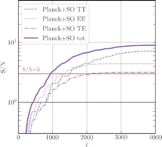
Combining Planck and SO can increase the total attainable S/N for boost detection to ∼9.
8 SUMMARY AND DISCUSSION
In this paper, we reviewed how the motion of the observer affects the statistics of the CMB radiation, expanding previous studies in various ways. We adopted a more careful boosting methodology, which is also applied to polarization maps and spectra. We clarified how deboosting can and should be performed, and we assessed how boosting effects could be exploited in future experiments to measure our peculiar motion with respect to the CMB. This paper also introduces COSMOBOOST : software aimed at accurately simulating the Doppler and aberration effects, or correcting/removing their footprints from observations.
We investigated the significance of the Doppler and aberration effects – induced by a dimensionless velocity β = 0.001 23 towards |$\hat{\boldsymbol \beta }=(264^\circ , 48^\circ)$| – on CMB statistics. The summary of the main results is as follows.
8.1 Boost variance
The motion of the observer changes the variance of the CMB anisotropies around the theoretical mean. Using simulations, in Section 3.3, we showed that the boost variance in an area towards the direction of motion (|$f_{\rm sky} = 10 {{\ \rm per\ cent}}$|) becomes larger than 10 per cent of the rest-frame cosmic variance in temperature, and 20 per cent in polarization beyond ℓ′ ≳ 1500. However, if the effect of the boost is being corrected in the theoretical mean, the boost variance reduces by an order of magnitude. We showed that the correction to the mean does not convey all the information on Cℓ modes in an individual (boosted) observation. We suggested the use of COSMOBOOST to correct boosting effects on the spherical harmonics, and we provided practical advice on how to perform the correction to the CMB power spectrum without using this software.
8.2 Hemispherical power asymmetry
In small patches of the sky towards (opposite to) the direction of motion, the induced coupling between harmonic multipoles increases (decreases) the power in both temperature and polarization up to a few per cent. In Section 4, we showed that this difference in power results in a hemispherical asymmetry in Planck-like simulations with an average (maximum) of roughly 1.0 per cent (1.7 per cent) in TT and 0.9 per cent (2.1 per cent) in EE (see Fig. 5). The motion-induced distortions in the power spectra (|$\propto \textrm{{d}}{\boldsymbol {\mathbb {C}}}_{\ell }/{\boldsymbol {\mathbb {C}}}_\ell$|) are out of phase with the primary CMB fluctuations; therefore, any hemispherical asymmetry of this origin is expected to show a similar fluctuating pattern. We made a comparison between the scale-dependent fluctuations in the power asymmetry of the Planck SMICA spectra and the ones from boosted simulations. The marginal resemblance between the oscillating patterns in the observation and simulations suggests that part of the hemispherical asymmetry observed in Planck SMICA maps could be due to the Doppler and aberration effects. However, we do not draw final conclusions and postpone a more rigorous analysis of this effect to future work.
8.3 Parity asymmetry
An analysis of the whole-sky boosted and rest-frame simulations revealed that the motion of the observer does not induce any parity asymmetry in neither temperature nor polarization of the CMB. In Section 5, using the R statistic, which calculates the ratio of even (ℓ = 2n) to odd multipoles (ℓ = 2n + 1), we found only a motion-induced parity asymmetry of the order of a few per cent of the standard deviation in rest-frame simulations in both TT and EE, for ℓmax = 500. Therefore, we safely reject Lorentz boost as a source of the anomalous parity asymmetry observed in Planck maps.
8.4 Planck cosmological parameter estimation
In Section 6, we revisited the impact of the boost on the Planck cosmological parameter estimation in light of a more precise boosting scheme, accurate mask consideration, and inclusion of polarization spectra. The bias implied by a neglected boost correction is only about 0.02σ on most parameters, with the most (least) affected being the sound horizon θ at 0.06σ (the amplitude of curvature perturbation As at 0.01σ). Therefore, the inclusion of these sophistications in the analysis shows even smaller biases on parameters than the ones reported in Catena & Notari (2013).
8.5 Boost detection
The motion-induced coupling between nearby harmonic multipoles can be exploited to measure our peculiar velocity with respect to the CMB rest frame in a different way from observing the CMB dipole. While Planck has measured our peculiar velocity using only TT spectra up to l ≃ 2000 (Aghanim et al. 2014), future experiments like SO and CMB-S4 could also leverage on polarization information (albeit on a smaller area of the sky). The signal, which is proportional to the slope of the underlying power spectrum, is intrinsically larger in EE polarization than TT. In Section 7, we showed that exploiting the high-temperature and polarization sensitivity of SO will allow us to obtain S/N ∼ 8.5, and S/N ∼ 9 in combination with Planck. CMB-S4 can enhance this measurement to S/N ∼ 20. These measurements combined with other probes of the the local motion of the Solar system such as galaxy number counts (Pant et al. 2019) and Sunyaev--Zeldovich (SZ) clusters (Chluba et al. 2012) will ultimately yield a Dipole-independent measure of our motion w.r.t. the CMB.
ACKNOWLEDGEMENTS
We are sincerely grateful to Daniel Lenz, Thejs Brinckmann, Lukas Hergt, Antony Lewis, and Nareg Mirzatuny for their incredible help with technical aspects of the project. We thank Loris Colombo, Emmanuel Schaan, and Colin Hill for helpful comments and discussions. We are also extremely thankful to the anonymous referee for their helpful comments on our manuscript. EP is supported by NASA 80NSSC18K0403 and the Simons Foundation award number 615662; EP and SY are supported by NSF AST-1910678. We acknowledge the use of the following software: CAMB (Lewis et al. 2000), Healpix (Górski et al. 2005), NaMaster Alonso et al. (2019), MontePython 3 (Audren et al. 2013; Brinckmann & Lesgourgues 2018), and GetDist (cmbant/getdist). Computations for this work were supported by the Center for High-Performance Computing (HPC) at the University of Southern California.
Footnotes
This can be interpreted as power leaking to higher multipoles in the direction of motion.
 syasini/CosmoBoost
The polarization power spectrum EE fluctuates with a larger slope than the temperature power spectrum TT.
To put it simply and perhaps more intuitively, it takes more aberration effect to make the quadrupole look like the octupole (ℓ = 2 → ℓ′ = 3) than it does for ℓ = 1000 → ℓ′ = 1001. Therefore, for the sameβ the former would be a smaller effect than the latter – i.e. aberration affects smaller scales more strongly than large scales.
We assume that equation (8) holds for an individual realization |$\tilde{C}_{\ell ^{\prime }}$|.
The fact that the |$\mathcal {O}(\beta ^2)$| effect drops only by a factor of 5 w.r.t. the |$\mathcal {O}(\beta)$| effect – not 1/β ≈ 800 as naively expected – results from the high degree of non-linearity of the Doppler and aberration kernel.
cmbant/CAMB
LSSTDESC/NaMaster
We checked with simulations and found that up to ℓmax = 3000, the formula captures the contribution of the first four neighbours with 0.1 per cent accuracy.
The accuracy of this estimation was not checked with simulations.
For simplicity, in this subsection, we do not use the prime accent for variables in the boosted frame.
REFERENCES
APPENDIX A: DOPPLER AND ABERRATION KERNEL
For reference, here we explicitly write the expressions for the temperature and polarization Doppler and aberration kernels. Detailed discussions on the topic can be found in Challinor, Ford & Lasenby (2000), Chluba (2011), Dai & Chluba (2014), and Yasini & Pierpaoli (2017b).
APPENDIX B: TE CROSS-CORRELATION
B1 Equal-area strip cuts
In order to gauge the significance of the motion-induced effects in the TE power spectrum, we repeat the exercise of Section 3 on the five equal-area strip cuts in the Northern hemisphere. Fig. B1 shows the relative change in the TE cross-correlation of 100 simulations for each of these strips, as well as the Jeong approximation and the 1σ region of the residuals it leaves in the power spectrum. Unlike TT and EE (see Fig. 2), there is no significant increase in the overall power as we go to smaller angular scales. However, similar to TT and EE, the amount of fluctuation increases as we go to higher latitudes (closer to the direction of motion). The Jeong et al. (2014) formula is still performing well for the change in the TE power spectrum, but it still leaves residuals for individual simulations.
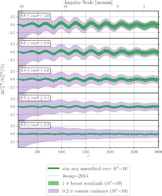
The relative change in the TE power spectrum due to the observer’s motion. The amplitudes of fluctuations are comparable to TT and EE cases, but unlike them there is no overall increase in power at smaller scales for TE. Similar to TT and EE, the Jeong et al. (2014) formula (dashed cyan) emulates the average effect extremely well, but leaves residuals in individual power spectrum realizations (green band). The residuals can be as large as 20 per cent of cosmic variance (purple band).
B2 Hemispherical asymmetry
Let us look at the amount of hemispherical asymmetry induced in TE due to the motion of the observer. Fig. B2 shows the amount of induced asymmetry in the Northern and Southern hemispheres, as well as the difference between the two. Similar to TT and EE, there is about |$\sim 1\!-\!2{{\ \rm per\ cent}}$| motion-induced hemispherical asymmetry in the TE power spectrum in the average of 100 simulations.
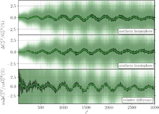
The observer’s motion induces an increase in power in the Northern hemisphere (top) and a decrease in the Southern hemisphere (bottom), which results in an overall |$\sim 1\!-\!2{{\ \rm per\ cent}}$| hemispherical asymmetry in the TE power spectrum. The faint green lines in the background are individual simulations, the jagged black line is the ensemble average, and the smooth green line is the average Gaussian smoothed over δℓ′ = 10. The statistic in the bottom panel is the same as the one in equation (16) with |$G_{\ell ^{\prime }}$| replacing |$C_{\ell ^{\prime }}$| in the denominator.
Similar to what happens in the case of TT and EE, the effects on the Northern hemisphere cancel out the ones in the Southern hemisphere upon the calculation of the power over the whole sky (see Fig. B3). The average change in TE drops to about 0.02 per cent in the whole-sky power spectrum.
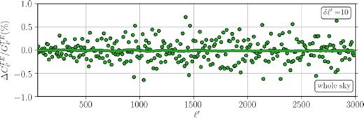
The motion-induced effects on each hemisphere cancel each other out when calculating the power spectrum on the whole sky.
B3 Planck SMICA
Finally, in Fig. B4 we look at the difference between the TE power spectra in the Northern and Southern hemispheres of the Planck SMICA maps and compare them to the boosted simulations. Similar to the case of TT and EE (Fig. 6), the fluctuations in the hemispherical asymmetry of SMICA TE resemble those of the simulations, which suggests that this difference could be at least due in part to the Doppler and aberration effects. We will look at this possibility closely in future work.
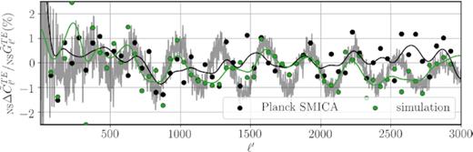
Comparison of Planck SMICA TE hemispherical asymmetry with simulations. The grey lines are the average of 100 simulations, the green circles and lines are a randomly chosen simulation binned and Gaussian smoothed over δℓ′ = 50, and the black circles and lines are the corresponding variables for Planck SMICA. The similarity between the fluctuation patterns of the two lines is certainly suggestive of the Doppler and aberration leftovers in the SMICA TE spectrum.
