


ABSTRACT
This paper studies pseudo-bulges (P-bulges) and classical bulges (C-bulges) in Sloan Digital Sky Survey (SDSS) central galaxies using the new bulge indicator ΔΣ1, which measures relative central stellar-mass surface density within 1 kpc. We compare ΔΣ1 to the established bulge-type indicator Δ〈μe〉 from Gadotti (2009) and show that classifying by ΔΣ1 agrees well with Δ〈μe〉. ΔΣ1 requires no bulge–disc decomposition and can be measured on SDSS images out to z = 0.07. Bulge types using it are mapped on to 20 different structural and stellar-population properties for 12 000 SDSS central galaxies with masses 10.0 < log M*/M⊙ < 10.4. New trends emerge from this large sample. Structural parameters show fairly linear log–log relations versus ΔΣ1 and Δ〈μe〉 with only moderate scatter, while stellar-population parameters show a highly non-linear ‘elbow’ in which specific star formation rate remains roughly flat with increasing central density and then falls rapidly at the elbow, where galaxies begin to quench. P-bulges occupy the low-density end of the horizontal arm of the elbow and are universally star forming, while C-bulges occupy the elbow and the vertical branch and exhibit a wide range of star formation rates at a fixed density. The non-linear relation between central density and star formation rate has been seen before, but this mapping on to bulge class is new. The wide range of star formation rates in C-bulges helps to explain why bulge classifications using different parameters have sometimes disagreed in the past. The elbow-shaped relation between density and stellar indices suggests that central structure and stellar populations evolve at different rates as galaxies begin to quench.
1 INTRODUCTION
The centres of galaxies are uniquely interesting regions of the universe. They are the bottoms of the deepest potential wells, they have the highest baryon densities on kiloparsec scales, they form stars under conditions that are very different from galactic discs, and they enable the growth of supermassive black holes. For all these reasons, we would like to understand their properties in detail.
Important information has emerged about galaxy centres from two rather different directions. The first approach has focused on centres as distinct objects and has studied them using multiple central properties such as morphologies, density profiles and other structural indices, stellar populations, dust and gas content, and star formation rates (e.g. Kormendy & Kennicutt 2004; Athanassoula 2005; Fisher 2006; Fisher & Drory 2008; Fisher, Drory & Fabricius 2009; Fisher & Drory 2010, 2011; Fabricius et al. 2012). A major result is that these disparate parameters are well enough correlated to justify a classification scheme that arranges galaxies into four bins – no-bulge systems, pseudo-bulges, classical bulges, and ellipticals – according to the prominence of a central, dynamically hot stellar population (Kormendy & Kennicutt 2004). Recent reviews of the criteria for classifying galaxies on this system are given by Fisher & Drory (2016, FD16) and by Kormendy (2016, K16).
The second approach attempts to reduce bulge structure to a single number, central stellar surface density within 1 kpc (Σ1). Previous work has shown two quite tight relations that separately describe star-forming galaxies and quenched galaxies in the Σ1–M* plane (e.g. Cheung et al. 2012; Barro et al. 2013; Fang et al. 2013; van Dokkum et al. 2014; Tacchella et al. 2015; Mosleh et al. 2017; Whitaker et al. 2017; Lee et al. 2018; Woo & Ellison 2019). An advantage of Σ1 is that it does not require high angular resolution or bulge–disc decomposition, which enables simple and robust measurements to be made out to z = 0.07 in Sloan Digital Sky Survey (SDSS; Fang et al. 2013) and to z = 3 in CANDELS (Barro et al. 2017), distances where the standard bulge-classification method cannot be used reliably with current data. In return for accepting less detailed information about the centres, the Σ1 method has been able to assemble large, volume-limited data sets that better illuminate connections with global properties and evolutionary trends. A major finding is that the two separate scaling laws that relate Σ1 to galaxy mass M* for quenched and star-forming galaxies have remained very similar since z = 3 (Barro et al. 2017). It thus appears that the manner in which galaxies build their central densities is an ancient process that has been in place for a long time.
The first purpose of this paper is to compare the Σ1 and pseudo-bulge/classical-bulge approaches. Do they order galaxies by central properties in the same way? A problem with the pseudo-bulge/classical-bulge method is that multiple criteria sometimes disagree. Which criteria, if any, correlate best with Σ1, and why? Is Σ1 by itself a useful bulge classifier for SDSS when comparing it to SDSS indices that have not been used for bulge studies before? Finally, do recent insights on galaxy evolution from SDSS and other large surveys shed light on how bulges are evolving?
Fig. 1 plots the Σ1–M* relation and three other structural relations for a sample of nearby SDSS galaxies. The greyscale represents the number density weighted by a completeness correction that is described below. Two features are apparent. One is the extreme narrowness of the Σ1–M* relation. Since galaxies grow significantly in mass, they must also increase in Σ1 in order to stay on this relation; in other words, the Σ1–M* relation for star-forming galaxies is an approximate evolutionary track (Barro et al. 2017). The white arrow shows this schematically. The second feature is two ‘islands’, seen strongly in three of the panels and separated by a weak valley. For concentration and global Sérsic index, the upper island is associated with quenched early-type galaxies while the lower island is associated with star-forming galaxies. It has been shown that the upper island/ridgeline in Σ1–M* also consists mainly of quenched and near-quenched galaxies, while the lower Σ1 island consists mainly of star-forming galaxies (e.g. Cheung et al. 2012; Fang et al. 2013; van Dokkum et al. 2014; Barro et al. 2017). It is also known that star formation rates divide massive galaxies into the red sequence and blue cloud, which are separated by the green valley (GV) (e.g. Strateva et al. 2001; Blanton et al. 2003; Kauffmann et al. 2003a; Bell et al. 2004; Faber et al. 2007; Wyder et al. 2007; Bell 2008; Brammer et al. 2009, 2011). The three valleys seen in Fig. 1, however, are based on structure, not star formation rates, and Section 7.3 will show that the membership of galaxies in the Σ1 islands is not exactly the same as membership in the red sequence and blue cloud. More precisely, the islands contain all the red, quenched galaxies, but they contain additional star-forming galaxies as well. A structural division similar to that shown here was seen in plots of concentration and Sérsic index versus stellar-population indices (Kauffmann et al. 2003b; Baldry et al. 2006; Driver et al. 2006; Ball, Loveday & Brunner 2008), but the difference between it and the stellar-population GV division was not stressed. We call this new feature the structural valley (SV) to distinguish it from the GV of star formation, and its relationship to pseudo-bulges and classical bulges is discussed in Section 7.3.
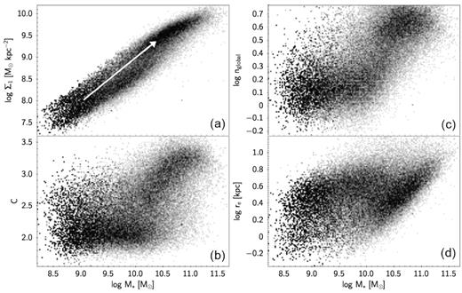
Panels (a), (b), (c), and (d) plot Σ1, concentration, global Sérsic index, and radius versus stellar mass for face-on, central, non-interacting SDSS galaxies with 0.02 < z < 0.07 as described in Table 1 (49 567 objects). The greyscale represents the number density weighted by the completeness correction; all bulge types are included. Two features are apparent. Note the narrowness of the Σ1–M* relation, as well as the two ‘islands’ seen most strongly in Σ1, concentration, and global Sérsic index. The upper ridgeline in panel (a) is populated mainly by quenched and quenching galaxies (Fang et al. 2013; Barro et al. 2017), but the islands in this figure are based on structure, not star formation rate, and their membership is not exactly the same as the red-sequence/blue-cloud division based on star formation. We have named the valley here the SV to distinguish it from the GV of star formation. The arrow represents a schematic evolutionary track in Σ1 versus M*.
It would seem from Fig. 1(a) that galaxies in general are evolving along the Σ1–M* relation (see the arrow), and therefore that Σ1 must increase during a galaxy’s lifetime. Furthermore, since the number of quenched galaxies is also increasing with time (e.g. Bell et al. 2004; Faber et al. 2007), there must be a net flow of galaxies all along the track, including from the main branch on to the upper island. The remainder of this paper will show that the Σ1 track encompasses all bulge types, from no-bulges and pseudo-bulges at the low-Σ1 end to classical bulges and ellipticals on the island. This implies that galaxies generally evolve smoothly in bulge type as well as Σ1, but previous literature on bulge types has not usually emphasized this possibility. Rather, a frequent picture for the origin of bulge types envisions separate mechanisms whereby pseudo-bulges (hereafter P-bulges) form from no-bulges (hereafter N-bulges) by internal secular evolution of galaxy discs whereas classical bulges (hereafter C-bulges) form via major mergers (FD16; K16), which not all galaxies would necessarily undergo. Another proposal is that C-bulges form early via gas-rich instabilities and mergers (e.g. Elmegreen, Bournaud & Elmegreen 2008; Dekel, Sari & Ceverino 2009; Forbes et al. 2014; Ceverino et al. 2015) while P-bulges form more gradually over time, undisturbed, in less dense regions (FD16). If this were strictly true, C-bulges and P-bulges would be on separate evolutionary paths, and P-bulges might again not evolve into C-bulges. Yet a third picture retains secular evolution and mergers as separate mechanisms but varies their importance smoothly with time and mass. When galaxies are low mass and gas rich, it is said that mergers have a limited ability to build stellar bulges (Robertson et al. 2006), and secular evolution is the major bulge-building mechanism. As mass grows and gas content declines, mergers are increasingly able to puff discs into hot stellar systems, and bulges begin to grow mainly by mergers (Hopkins et al. 2009a, b). This version of the two-mechanism picture allows – even requires – that many P-bulges would evolve into C-bulges. Indeed, Kormendy et al. (2010) wondered whether mergers are so effective that all massive galaxies should by now have developed C-bulges, contrary to what is seen.
In contrast to the multiple bulge-building paths entertained in the bulge-classification literature, the Σ1 literature has stressed an unbroken continuum in which all galaxies are continuously building their centres in basically the same fashion, as envisioned in the bulge-evolution picture. However, not much attention has been paid in this literature to the detailed mechanism(s) that does this. Fang et al. (2013) and K16 have stressed that the rise of Σ1 is a natural consequence of entropy growth in self-gravitating systems whereby a multitude of processes – such as violent relaxation, disc instabilities, and gravitational interactions between bars, spirals arms, and stars, etc. – permit subcomponents to exchange energy and angular momentum among themselves, inevitably driving up central density while at the same time building an extended outer envelope. Gaseous dissipation involves actual net energy loss on top of this and compounds the concentration process still further, especially at early times when galaxies are gas rich and dissipative compaction can occur (Dekel et al. 2009; Zolotov et al. 2015; Barro et al. 2017). Although there are mechanisms that can reduce Σ1, their effect is generally small, and they mostly occur after a galaxy is quenched (van Dokkum et al. 2015; Barro et al. 2017). Thus, according to this picture, Σ1 acts as a kind of clock for galaxy evolution: it can easily go up, but it can never go down (by very much).
The previous discussion has glossed over an important point, namely that P-bulges are actually of two types: boxy/peanut bulges, which form via vertical dynamical instabilities in a bar, and discy bulges, which form from gas brought to the central regions via secular evolution (Kormendy & Kennicutt 2004; Athanassoula 2005). These two types of bulges may affect different bulge indicators differently, and we return to the question of barred versus unbarred galaxies in Section 4.
We further note that even though galaxies may be evolving through the various bulge types, not all massive galaxies have evolved all the way to the C-bulge or elliptical stage. Many nearby massive galaxies have P-bulges, e.g. NGC 1097 and M51 (Kormendy & Barentine 2010; Kormendy et al. 2010; Kim et al. 2014; Salo et al. 2015; Gadotti et al. 2019; Querejeta et al. 2019); see also Fig. 16 below. Why some massive galaxies may have evolved to earlier bulge types but others have not is an open question; the data from this study may help to answer it.
Since valuable information about galaxy centres has come from both the Σ1 and bulge-classification approaches, the first goal of this paper is to see whether the two approaches agree. To accomplish this, a sample of objects is needed that has been classified both ways. Fortunately, such a sample is available from the work of Gadotti (2009, G09), who measured bulge types for nearly 1000 SDSS galaxies based on Δ〈μe〉, one of the classic parameters used to classify galaxies in the bulge-classification method (see Section 2 for the definition of Δ〈μe〉). Section 4 compares Δ〈μe〉 to ΔΣ1 (which is Σ1 with mass trend removed), and it appears that both parameters measure approximately the same thing, namely central stellar mass density.
Having established that ΔΣ1 is a valid indicator for SDSS bulges, we then move on to the second part of the paper, which maps 20 different SDSS properties on to bulge types for ∼12 000 SDSS galaxies. New trends emerge from this large and homogeneous sample. The main result is that structural parameters are generally found to correlate closely with ΔΣ1, which is itself a structural parameter, but that spectral indices of C-bulges are bifurcated, with some C-bulges being quenched and others (very) actively star forming. This is consistent with previous studies of star formation rate as a function of ΔΣ1 and helps to explain why the classification of C-bulges has proved difficult – they are not a homogenous class. The bottom line is that the structure and stellar populations of bulges are highly correlated, but not in a linear fashion.
This paper is organized as follows. The data and sample selection are described in Section 2. Section 3 uses the SV to determine the trend of Σ1 versus mass and defines a residual ΔΣ1 relative to the valley. ΔΣ1 is our preferred parameter to characterize the structural state of galaxy bulges. It is compared to the traditional parameter Δ〈μe〉 in Section 4 using the G09 sample, and agreement is generally good. Further comparisons in Sections 5 and 6 reinforce this using 20 structural and stellar-population parameters from SDSS and other data. Finally, Sections 5 and 6 show trends for the whole SDSS sample in the mass range 10 < log M*/M⊙ < 10.4. Implications are discussed in Section 7, and a summary is given in Section 8. Unless otherwise noted, all structural measurements are based on the SDSS i band. We adopt a concordance ΛCDM cosmology: H0 = 70 km |$\rm s^{-1}\ Mpc^{-1}$|, Ωm = 0.3, and |$\Omega _\Lambda$| = 0.7.
2 DATA AND SAMPLE SECTION
Two main samples of galaxies are used in this paper. The first is a large SDSS sample used to study the general properties of galaxies versus central density. It is selected from the SDSS DR7 catalogue (Abazajian et al. 2009). To avoid seeing degradation, we limit the redshift range to 0.02 < z < 0.07 (Fang et al. 2013). Besides the redshift cut, galaxies are limited to log M*/M⊙ > 9.5, axial ratio b/a > 0.5, and single-Sérsic index 0.5 < n < 6. The decision was also made to focus on central SDSS galaxies for this first analysis. It is known that environment affects both stellar populations (e.g. Blanton & Moustakas 2009; Woo et al. 2015) and structural properties (Woo et al. 2017), but the detailed mechanisms are not yet known. We therefore prefer to use the simpler life histories of field galaxies to formulate a basic picture of bulge properties, against which satellite galaxies can be compared in future work. Satellite galaxies are accordingly excluded based on the group designation (Mrank > 1) according to Yang et al. (2012). Merging galaxies are also excluded for similar reasons, using the classification (PMG < 0.1) from Galaxy Zoo (Lintott et al. 2011). After applying these criteria, 41 272 objects are left in this sample.
Integrated photometry (model magnitude) and surface brightness profiles in the ugriz bands for SDSS galaxies are obtained from the SDSS data base and corrected for Galactic extinction. K-corrections are applied using the k-correction code v4.2 from Blanton & Roweis (2007). We compute the cumulative light profile and interpolate smoothly in order to calculate the total light within 1 kpc. The stellar mass surface density within 1 kpc, Σ1,1 is computed using the total light within 1 kpc in the i band and M/Li from Fang et al. (2013). We also add NUV magnitude for those galaxies that have observations in the GALEX data base and apply the Galactic correction and K-correction as for the SDSS photometry. Spectroscopic data including redshifts, stellar masses, fibre velocity dispersions, Dn4000, H δA, H α equivalent width, [O iii], H β, [N ii], H α fluxes, global SSFR, and fibre SSFR are obtained from the MPA/JHU DR7 value-added catalogue.2 We exclude galaxies whose spectra with median per-pixel S/N < 10 when using spectroscopic parameters. Structural parameters in the i band, such as concentration index (defined as R90/R50), global Sérsic index, and effective radius of the galaxies in kpc (converted from the single-Sérsic fit), are taken from the NYU Value-Added Galaxy Catalog (NYU-VAGC) DR73 (Blanton et al. 2005; Adelman-McCarthy et al. 2008; Padmanabhan et al. 2008). We also add the bulge–disc decompositions and b/a values from Simard et al. (2011). Internal reddening corrections from Oh et al. (2011) are applied to all colours but not to emission lines or to absorption indices.
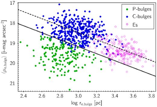
Mean bulge effective surface brightness versus bulge effective radius (Kormendy relation, Kormendy 1977) using data for SDSS galaxies derived from the catalogue of Gadotti (2009, G09). The green, blue, and magenta points indicate P-bulges, C-bulges, and ellipticals, respectively, as classified by G09. Δ〈μe〉 is the residual value of 〈μe〉 relative to the solid line (which is taken from G09). The dashed line above it schematically represents the ridgeline of galaxies identified by Kormendy (1977) as consisting of C-bulges and elliptical galaxies.
The bulge–disc–bar decomposition in G09 also included bars as separate structures. We elect to leave out the bar-component contribution to central density when computing ΔΣ1 for G09 galaxies, but we verify in Fig. 9 below that this choice has not moved barred galaxies systematically off the C-bulge correlation. In the interest of maximizing the number of galaxies, we have likewise retained both satellites as well as centrals in the G09 sample.
We preserve the bulge types from G09 when studying that sample, and this includes using his E classification. When studying the SDSS sample, it is desirable to retain the E/C-bulge distinction, but high-quality bulge–disc decompositions for SDSS are not available. Therefore, we use the probability of a galaxy being an elliptical, P(Ell), from Huertas-Company et al. (2011). Fig. 3 shows the P(Ell) histogram for the G09 sample as a function of G09 bulge type. N-bulges and P-bulges are well separated from E’s, but a large population of C-bulges overlaps with E’s, as shown in the figure. We tested the G09 sample extensively to see if any other structural parameter, such as SDSS concentration, B/T, global Sérsic index, velocity dispersion, or effective mass surface density, could be used to distinguish E-like C-bulges from true E’s, but found none that worked. We therefore elect to classify all SDSS galaxies with P(Ell) > 0.65 as E’s. N-bulges are rare in the G09 sample due to the lower mass limit log M*/M⊙ > 10. The plot of bulge frequencies in Fisher & Drory (2011) also indicates that N-bulges are rare when log M*/M⊙ > 10. Thus, we do not try to make the N-bulge/P-bulge division in this paper but rather simply group the G09 N-bulges in with the P-bulges.
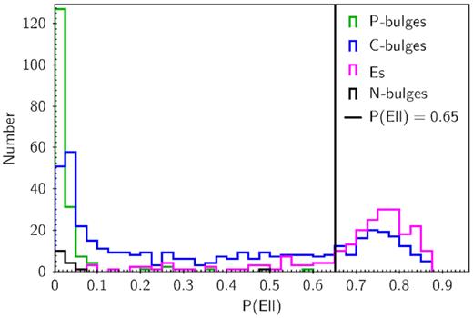
The histogram of the probability of a galaxy being an elliptical, P(Ell), for G09 galaxies. Probabilities are taken from the morphological study of Huertas-Company et al. (2011). The black, green, blue, and magenta histograms represent N-bulges, P-bulges, C-bulges, and E’s, respectively, based on the G09 classifications. N-bulges and P-bulges are cleanly distinguished from E’s, but C-bulges (blue line) are a mixture of types. We could not find any other measurable parameter to differentiate E-like C-bulges from true E’s in the G09 sample, and so all SDSS galaxies with P(Ell) > 0.65 (vertical line) are classed as E’s. N-bulges are classified by the definition of B/T = 0 in G09, which makes them rare in the G09 mass range.
The grey background in Fig. 4 shows the raw density distribution of SDSS galaxies with z < 0.1 in all mass ranges. The foreground plot in yellow shows the density plot for the final sample with all cuts applied. Significant volume-limited corrections are needed for both high-mass and low-mass galaxies (see the caption). We therefore calculate Vmax and Vmin for each object using its redshift and the SDSS survey limits 14 < r < 17.5, where Vmax and Vmin represent the maximum and minimum volumes, respectively, over which the object would be included in the survey. Each galaxy is assigned a completeness correction for both the bright and faint limits based on Vmax and Vmin. SDSS galaxies in all density plots in this paper are weighted by this correction. In much of what follows, a mass-limited SDSS subsample is selected with 10.0 < log M*/M⊙ < 10.4 to highlight masses where the structural bimodality is most prominent (cf. Fig. 1). This mass range is approximately 67 |${{\ \rm per\ cent}}$| complete in the range 10.0 < log M*/M⊙ < 10.1, 80 |${{\ \rm per\ cent}}$| complete in the range 10.1 < log M*/M⊙ < 10.2, and 100 |${{\ \rm per\ cent}}$| complete in the range 10.2 < log M*/M⊙ < 10.4. The selection criteria and resulting sample sizes are summarized in Table 1.
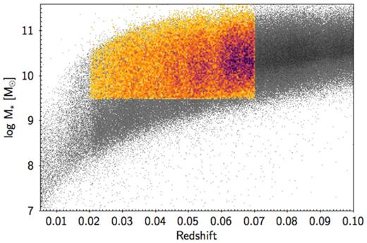
Stellar mass versus redshift, colour coded by raw number density. The grey background is all SDSS galaxies with z < 0.1 in all mass ranges, with upper and lower boundaries set by 14 < r < 17.5. The yellow foreground is our final SDSS sample (Table 1) with 0.02 < z < 0.07, M* > 109.5 M⊙, b/a > 0.5, centrals only, and good-quality single-Sérsic fits. The dark band marks quenched galaxies, which are not detected as deeply as star-forming galaxies on account of their red colours; some low-mass objects of this type are missed at high redshifts in the lower right corner of the yellow region. Conversely, the magnitude cut-off at upper left discriminates against high-mass objects at low redshifts. Significant volume-limited corrections are needed both below 1010 M⊙ and above 1011 M⊙ to correct for these effects (see the text).
Sample descriptions and sizes.
| Desciption | Criterion | N |
|---|---|---|
| SDSS samplea | ||
| Redshift limit | 0.02 ≤ z ≤ 0.07 | 156 634 |
| Magnitude limit | 14 ≤ r ≤ 17.5 | 136 271 |
| Face-on galaxies | b/a ≥ 0.5 | 84 656 |
| Good Sérsic fit | 0.5 < n < 5.9 | 80 098 |
| Central galaxies | Mrank = 1 | 53 519 |
| Non-interacting galaxies | PMG < 0.1 | 49 567 |
| SDSS sample | log M*/M⊙ > 9.5 | 41 272 |
| Mass-limited SDSS sampleb | 10 < log M*/M⊙ < 10.4 | 12 421 |
| G09 samplec | Galaxies from G09 | 860 |
Notes. aCross-matched with all mentioned catalogues.
bAbout 1000 galaxies with median per-pixel S/N < 10 in this sample are excluded when using spectroscopic parameters.
cCross-matched with all mentioned catalogues but without the criteria listed above.
To summarize, there are two main samples used in the remainder of this paper to compare bulge types to structural and spectral indices. One is the small G09 sample with high-quality bulge–disc decompositions. This sample of about 1000 galaxies covers all stellar masses above 1010 M⊙ and contains both central and satellite galaxies. The second is the much larger mass-limited SDSS sample in the range 1010.0–10.4 M⊙, which lacks accurate bulge–disc decompositions and consists of only centrals.
3 THE SV IN THE Σ1–M* DIAGRAM
When using Σ1 as a central density indicator for a wide range in stellar mass, it is important to remove any trend versus mass first. Fang et al. (2013) showed that the Σ1 ridgeline is tilted and that the threshold for quenching grows with stellar mass. Barro et al. (2017), Tacchella et al. (2015), and Lee et al. (2018) confirmed this out to z ∼ 3. All four studies fitted the ridgeline with a simple power law in log–log coordinates. With more careful inspection, we observe a slight curvature in Fig. 1(a) (repeated in Fig. 5b).
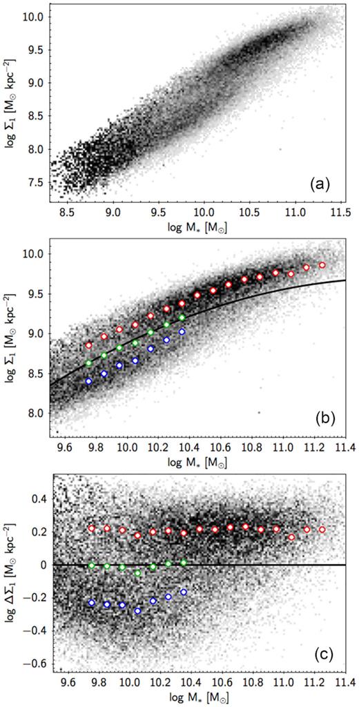
Panel (a): Σ1 versus stellar mass for all SDSS galaxies, ellipticals included, repeated for reference from Fig. 1(a). Panel (b): Σ1 versus stellar mass for the final SDSS sample with log M*/M⊙ > 9.5. Panel (c): ΔΣ1 versus stellar mass for the SDSS galaxies as in panel (b). The points in all the three panels are colour coded by number density weighted by the completeness correction. The red and blue points with white centres are the locations of the high-Σ1 and low-Σ1 populations determined by double Gaussian fitting (see Fig. 6). The location of the SV is indicated by the green points with white centres, which are half-way between the red and blue points. The solid black line in panel (b) is a parabola fitted to the ridgeline of the red points and shifted downward by 0.21 dex to match the SV. Its equation is in the text. ΔΣ1 is defined to be zero along this line, which flattens out the distributions versus mass.
A feature noted in Fig. 1 is a weak valley that separates quenched from star-forming galaxies. Fig. 5(a) repeats Fig. 1 for reference, and Fig. 5(b) is magnified to show more details at the high-mass end. Fig. 6 shows histograms of vertical slices through the population at representative masses (ellipticals have been deleted from these slices in order to better equalize the height of the two peaks), which show that the maximum depth is only about 15 |${{\ \rm per\ cent}}$|. As noted, in order to distinguish between the GV found in the colour–magnitude diagram and the new valley found in Σ1–M*, we have dubbed this feature the SV since Σ1 is a structural parameter, not a colour. The general trend, noted in the ‘Introduction’ section, of galaxies to evolve from star forming to quenched (e.g. Bell et al. 2004; Faber et al. 2007) then implies a net flow of galaxies evolving across the SV.
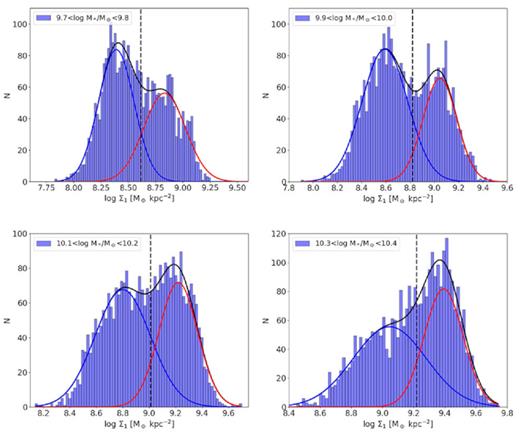
Histograms of Σ1 with fitted double Gaussians in four illustrative mass bins of SDSS: 9.7 < log M*/M⊙ < 9.8, 9.9 < log M*/M⊙ < 10.0, 10.1 < log M*/M⊙ < 10.2, and 10.3 < log M*/M⊙ < 10.4. Completeness corrections have been applied, and only bulges are counted (ellipticals are excluded). The red and blue lines are the individual Gaussians; the black lines are the sum. The black dashed lines show the valley, which is defined by the half-way point between the Gaussian centres.
To remove the mass trend, we fit double Gaussians to the slices shown in Fig. 6. The SDSS sample in Table 1 is used, E’s are excluded, and the volume-limited density correction is applied. Fig. 6 shows the fitting results for four illustrative mass slices: 9.7 < log M*/M⊙ < 9.8, 9.9 < log M*/M⊙ < 10.0, 10.1 < log M*/M⊙ < 10.2, and 10.3 < log M*/M⊙ < 10.4. A single Gaussian is used when log M*/M⊙ > 10.4 since the low-Σ1 galaxies are too few in these mass slices. The two populations are not strongly separated, but the peaks (and hence the SV) appear to be well located. The location of the SV at each mass is defined as the half-way point between the two Gaussian centres. This definition is adopted since it is more robust than the minimum itself to changes in the relative strengths of the peaks.
Fig. 5(c) shows the density plot of ΔΣ1 versus M*. All trends are now flat, and ΔΣ1 = 0 divides galaxies into the two structural clouds. There is a slight turn-up in the ridgelines at low mass, but Σ1 will be used only above log M* = 9.8, where the relations are quite flat. We will test ΔΣ1 as a new parameter to differentiate P-bulges from C-bulges. In our picture in which galaxies are moving in Σ1 and M* from lower left to upper right in Fig. 5(a) (Fang et al. 2013; Barro et al. 2017), ΔΣ1 is an evolving quantity that measures the distance of a galaxy from the final quenched ridgeline.
4 COMPARING Δ〈μe〉 AND ΔΣ1
The next three sections of the paper compare the new parameter ΔΣ1 to other variables, starting in this section with Δ〈μe〉 from G09, which was defined in Fig. 2. Recall that the G09 sample was selected to provide a calibration sample of SDSS galaxies with known bulge types. Therefore, we hope to find good agreement between ΔΣ1 and Δ〈μe〉 in this comparison.
Fig. 7 compares ΔΣ1 and Δ〈μe〉 versus stellar mass for the G09 galaxies. Points are colour coded according to the bulge classification in G09. The agreement with the coloured points is essentially perfect in the lower panel, as expected since the G09 bulge types are based on this parameter. However, the quenched ridgeline and SV are more clearly defined in ΔΣ1–M*. The C-bulge ridge is offset above using Δ〈μe〉 but superimposes closely using ΔΣ1. The latter agrees better with the claim by K16 that the bulges of strong C-bulges are identical to E’s (but see G09 for a different view). Δ〈μe〉 varies significantly with stellar mass, while ΔΣ1 is more constant, the mass trend having been removed. This contributes to the fact that Δ〈μe〉 tends to classify more galaxies as C-bulges at log M*/M⊙ > 10.5 and fewer galaxies as C-bulges at log M*/M⊙ < 10.5 than ΔΣ1. On the whole, however, the two parameters appear to be measuring the same thing, namely central density.
Panel (a): ΔΣ1 versus M* for G09 galaxies. Panel (b): Δ〈μe〉 versus M* for G09 galaxies. Points are colour coded according to the bulge classification in G09. The green and blue points represent P-bulges and C-bulges, respectively, and the magenta circles are E’s. The quenched ridgeline and the SV are more prominent in panel (a), and E’s are also located closer to the high-ΔΣ1 ridgeline. Overall, however, the two parameters appear to be measuring roughly the same thing, especially if the residual mass trends in Δ〈μe〉 were removed.
Fig. 8 shows examples of SDSS postage stamps for G09 galaxies with redshifts z ∼ 0.04 for two mass bins 10.0 < log M*/M⊙ < 10.2 and 10.4 < log M*/M⊙ < 10.6. Galaxies from top to bottom are arranged by their ΔΣ1 values. The two white circles in the upper left corner of the panels show the region where Σ1 is calculated. The smooth progression of morphology from the bottom to top row indicates that ΔΣ1 sorts galaxies well by bulge prominence, which is as expected since fig. 9 in Fang et al. (2013) has shown a similar morphology transition using Σ1. Ordering galaxies by Δ〈μe〉 gives substantially the same results (G09), further confirming the similarity of ΔΣ1 and Δ〈μe〉.
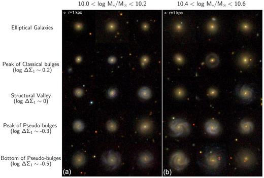
Sample SDSS postage stamps for G09 galaxies with redshifts z ∼ 0.04. Panel (a) shows galaxies with 10.0 < log M*/M⊙ < 10.2, and panel (b) shows galaxies with 10.4 < log M*/M⊙ < 10.6. The top row shows E’s according to G09 that also have P(Ell) > 0.65 according to Huertas-Company et al. (2011). The other four rows are arranged downward by ΔΣ1. E’s and C-bulges peak around log ΔΣ1 ∼ +0.2, while P-bulges peak around log ΔΣ1 ∼ −0.3. Galaxies with log ΔΣ1 ∼ 0 are in the SV. Galaxies with log ΔΣ1 ∼ −0.5 are at the bottom of the log ΔΣ1–M* diagram. The two white circles in the upper left corners have a radius of 1 kpc, which is the region where Σ1 is calculated. Similar figures were presented in Fang et al. (2013) and G09.
Finally, Fig. 9 plots ΔΣ1 versus Δ〈μe〉 directly for the G09 galaxies. ΔΣ1 follows Δ〈μe〉 fairly closely but with some scatter. Separate tests show that the residuals in this relation correlate mainly with galaxy radius and mass: Larger and more massive galaxies lie to the lower right. These systematic residuals are due in part to the fact that mass/size trends have been removed from ΔΣ1 but not from Δ〈μe〉 (see the discussion, Fig. 11), and if that were done, the agreement in Fig. 9 would tighten. In other words, the suspicion is that, by applying information from additional parameters, it should be possible to predict Δ〈μe〉 accurately from ΔΣ1. This is confirmed by the work of Yesuf et al. (2019), who use the random forest classifier to predict G09 bulge types from the SDSS data, achieving an accuracy of 95 per cent. As expected, ΔΣ1 has the highest feature importance, followed by concentration and fibre velocity dispersion.
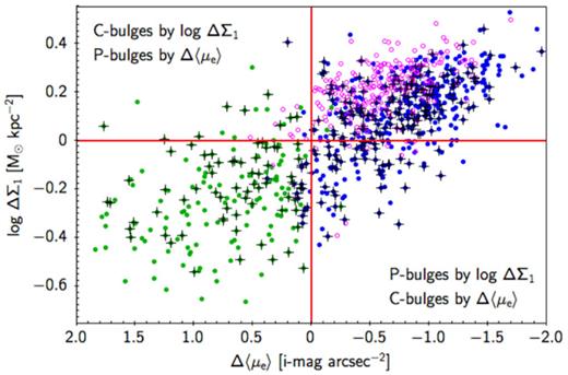
ΔΣ1 is compared directly to Δ〈μe〉 for the G09 galaxies. Points are colour coded according to the galaxy classifications in G09. The green points are P-bulges, the blue points are C-bulges, and the magenta circles are E’s. The reasonable agreement between ΔΣ1 and Δ〈μe〉 suggests that ΔΣ1 can substitute for Δ〈μe〉 as a bulge-classification parameter. Some disagreement occurs in the upper left and lower right quadrants, where types disagree. Separate tests show that the residuals correlate with galaxy mass and radius, reflecting the fact that the mass trend has been removed from ΔΣ1 but not from Δ〈μe〉 (cf. Fig. 7). The black crosses show barred galaxies according to G09. Their location relative to unbarred galaxies is discussed in the text.
Barred galaxies identified by G09 are indicated by the black crosses in Fig. 9. G09 models bars and bulges separately, but the Δ〈μe〉 parameter incorporates only the mass in bulges whereas ΔΣ1 uses the entire central mass. It is therefore important to check whether there is an offset between Δ〈μe〉 and ΔΣ1 as a function of bar presence. Fig. 9 shows generally no large difference between the two distributions aside from the well-known tendency of bars to inhabit galaxies with larger bulges and thus higher central densities (e.g. Masters et al. 2011). Any offset for barred versus unbarred galaxies should be larger for P-bulges, which have intrinsically lower surface brightness and would therefore be inflated more by the presence of bar light. However, the median value of Σ1 in barred P-bulges (green points) is only 0.06 dex (16 per cent) higher than that in non-barred P-bulges, which is small. We also checked for systematic differences between barred and non-barred galaxies in Figs 10–14 below but see none. We conclude that the effect of bars on our classification parameters is small.
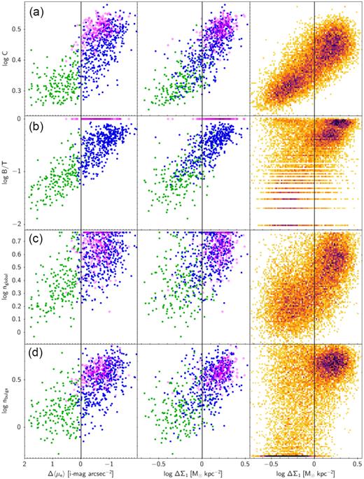
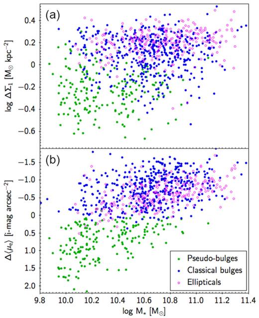
This figure compares four structural parameters versus the structural P-bulge/C-bulge indicators Δ〈μe〉 and ΔΣ1. The two plots on the left in each row compare Δ〈μe〉 and ΔΣ1 for the G09 sample, which includes both central and satellite galaxies. The green and blue points and magenta circles represent P-bulges, C-bulges, and E’s, respectively, as classified by G09. The vertical black lines are the adopted boundaries in ΔΣ1 (here) and Δ〈μe〉 (in G09) that divide P-bulges from C-bulges according to each criterion (P-bulges are to the left of the line in each plot). The rightmost plots are the same structural parameters versus ΔΣ1 for the mass-limited SDSS central sample. SDSS points are weighted by the completeness correction computed in Section 2; E’s are included in the SDSS sample but are not separately marked. The stellar mass, b/a, and redshift limits of the G09 sample are log M*/M⊙ > 10, b/a > 0.9, and 0.02 < z < 0.07, respectively, while the stellar mass, b/a, and redshift limits of the mass-limited SDSS sample are 10.0 < log M*/M⊙ < 10.4, b/a > 0.5, and 0.02 < z < 0.07, respectively. The lower masses in SDSS explains why some parts of the diagrams are not populated (e.g. high values of C are missing). B/T and nbulge for the bulges of G09 galaxies are from the decomposition data in G09, while B/T and nbulge for the galaxies in the SDSS sample are from Simard et al. (2011). A group of galaxies was originally seen in the upper left corner of the SDSS sample in panel (b). Many are objects for which the fitting procedure misidentified bulges as discs and vice versa (e.g. Simard et al. 2011). They are omitted from panels (b) and (d). The outlier population in this region of panel (b) is thereby reduced but still not entirely removed.
In summary, Figs 7–9 collectively imply that ΔΣ1 and Δ〈μe〉 both measure central density and that ΔΣ1 is therefore a reasonable substitute for Δ〈μe〉 as a bulge-classification parameter. This finding agrees with previous works that have also found that central density is closely correlated with bulge type (e.g. Carollo 1999; Fisher & Drory 2016). Unlike Δ〈μe〉, ΔΣ1 does not require bulge–disc decomposition and can be measured directly from SDSS images out to z = 0.07. The use of ΔΣ1 therefore opens the way to studying bulge properties using the full statistical weight of SDSS.
5 Δ〈μe〉 AND ΔΣ1 COMPARED TO OTHER STRUCTURAL PARAMETERS
This section compares Δ〈μe〉 and ΔΣ1 to other structural parameters. Many of these have been mentioned in the literature as useful discriminators between P-bulges and C-bulges (e.g. K16). The comparisons are illustrated in Figs 10–11. Each parameter is shown with three plots. The left and middle plots show the G09 galaxies coloured by bulge types from G09. The leftmost panel uses Δ〈μe〉 from G09, while the middle panel uses ΔΣ1. The far right plot repeats ΔΣ1 for the mass-limited SDSS sample from Table 1 with 10.0 < log M*/M⊙ < 10.4, where SDSS is nearly complete. Ellipticals are included in all the plots but they are not separately marked in the SDSS sample; in this mass range, they are a minority of galaxies, even in the evolved ridgeline population.
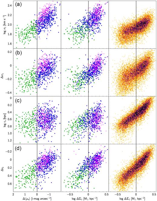
Two additional structural parameters are compared to Δ〈μe〉 and ΔΣ1. The format is the same as Fig. 10. The Y-axis is reversed for re and Δre to match the sense of other figures. The quantity σ1 is the velocity dispersion scaled to a circular aperture of radius 1 kpc, which is computed from the SDSS fibre velocity dispersion using the relation σ ∝ r−0.066 according to Cappellari et al. (2006). Note the lack of high-σ1 galaxies and the lower scatter in the mass-limited (and central) SDSS sample due to the lack of massive galaxies. Velocity dispersion and effective radius of the galaxies (global) are shown raw and with mass trends removed by fitting and subtracting the ridgeline relations for quenched galaxies versus mass. The use of such residuals is appropriate when using ΔΣ1, which also has its mass trend removed. The scatter is accordingly reduced for ΔΣ1 in panels (b) and (d) for the G09 sample, which has a large mass range.
To homogenize the appearance of the plots, the Y-axes are inverted as needed to place quenched galaxies at the top and star-forming galaxies at the bottom. The vertical black lines divide bulge types: Galaxies to the left of these lines are classed as P-bulges and galaxies to the right are C-bulges, according to which X-axis parameter is used. The basic source of all data unless otherwise stated is SDSS DR7 (Abazajian et al. 2009). Any additional special treatments are described in the captions and the text below.
Before describing the figures in detail, we remind readers of our picture that galaxies are on average evolving from low central density to high central density, and thus that there is a net flow of galaxies over time in each figure from left to right. The basis of this point is Fig. 1(a), where the narrowness of the Σ1 locus establishes its nature as an approximate evolutionary track along which Σ1 and stellar mass both grow with time. A further implication is that galaxies must also on average be moving across the SV, which is implied by the steadily increasing number of galaxies on the Σ1 ridgeline from z = 2.5 to now (Barro et al. 2017).5 The important conclusion is that, if bulge type is based on central stellar density (i.e. ΔΣ1 or Δ〈μe〉), at least some P-bulges are evolving to become C-bulges. This answers a major question set up in the ‘Introduction’ section, namely how bulge types relate to galaxy evolution. However, a small caveat is necessary. Many of the following figures show prominent ridgelines, and it is tempting to interpret these as actual evolutionary tracks, analogous to the giant-branch ridgelines in HR diagrams. Although this is very broadly true, future papers will show that the ridgelines in Figs 10–14 are in fact composites of different galaxy subpopulations, and individual galaxies do not necessarily evolve all the way from the far left to the far right in each diagram.
We start with Fig. 10, which displays correlations with four structural parameters measured from the galaxy images.
10(a), log C (R90/R50): The agreement between log C (concentration) and Δ〈μe〉 and ΔΣ1 is one of the best among all the panels, showing few discrepant galaxies off the main relations in the lower right or upper left corners. ΔΣ1 (correlation coefficient r = 0.79) is a bit tighter than Δ〈μe〉 (r = −0.75), but both the parameters are well correlated. The use of log on the Y-axis (and in the other panels) matches the use of logs on the X-axis. The consistent use of logs on both the axes makes all structural diagrams look roughly like power laws. The SDSS sample at right shows an extra blob (more accurately, a widening) at log C ∼ 0.44 and ΔΣ1 ∼ +0.3 that is not seen in the G09 sample (perhaps, this is due to the fact that there are too few galaxies in the G09 sample). This is an example of a subpopulation, and future papers will show that this feature is associated with the smallest quenched galaxies in this SDSS mass range. Values of C in the SDSS sample do not reach the highest values present in the G09 sample owing to the mass limit at log M*/M⊙< 10.4 in SDSS.
10(b), log B/T: The two left plots use log B/T values from G09. Both are tight, with ΔΣ1 (r = 0.76) comparable to Δ〈μe〉 (r = −0.75). The absence of galaxies above log B/T = −0.01 is due to the fact that G09 places all high-B/T objects in the elliptical category, which are shown as the magenta circles at the top of the panels. The SDSS panel uses B/T from Simard et al. (2011). The discontinuity for the low-B/T galaxies is due to the fact that Simard et al. (2011) do not use three decimal digits for B/T. A group of galaxies was originally seen in the upper left corner of the SDSS sample. Many of these proved to be objects in which the fitting procedure misidentified bulges as discs and vice versa (e.g. Simard et al. 2011). Their B/T values were much too high, and they are omitted from this panel (and also from panel d). The outlier population is consequently reduced but is still not entirely eliminated. Agreement between B/T and ΔΣ1 is much poorer overall for SDSS than for the G09 sample, possibly indicating less accurate bulge–disc decompositions in Simard et al. (2011).
10(c), log nglobal: All nglobal indices are single-Sérsic fits from the NYU-VAGC. In the G09 plots at left, Δ〈μe〉 (r = −0.65) now is tighter than ΔΣ1 (r = 0.52), but the scatter in both the plots is large. The SDSS and G09 samples look basically the same, but high-n values are missing from SDSS, a consequence of the 1010.4 M⊙ upper mass limit.
10(d), log nbulge: The two left plots use nbulge from G09. Both relations have intermediate tightness, and Δ〈μe〉 (r = −0.67) is slightly tighter than ΔΣ1 (r = 0.61). The SDSS panel uses nbulge from Simard et al. (2011). The vertical distribution is very different from G09, there being many more low-nbulge objects in SDSS. This again is due to the low-mass cut in SDSS. The tail of outliers in the upper left corner that is visible in panel (b) is present here too. Even though nbulge < 2 (log nbulge < 0.3) has been used as a prime pseudo-bulge discriminant in the past (Fisher & Drory 2008), G09 gave it low weight based on poor agreement with his Δ〈μe〉. This scatter is visible in the far-left panel using Δ〈μe〉 and is replicated using ΔΣ1 in the middle panel. Much of this is probably intrinsic, but an additional factor is that nbulge (and B/T) depends on bulge–disc decompositions. The large scatter for SDSS here parallels the similar scatter in panel (b) and suggests less accurate bulge–disc decompositions in Simard et al. (2011).
Several conclusions follow from Fig. 10. The most important is that both Δ〈μe〉 and ΔΣ1 show reasonable correlations with other well-measured structural parameters and that ΔΣ1 correlates comparably to Δ〈μe〉 with these other measures. The second point is that bulge types using Δ〈μe〉 versus ΔΣ1 agree well. It is true that a few galaxies are on different sides of the vertical lines in the two left-hand panels, but this is a detail – the major features of both diagrams are the same. We therefore feel comfortable in generally denoting P-bulges as low-density bulges and C-bulges as high-density bulges without having to specify which measure, Δ〈μe〉 or ΔΣ1, we are using. If it matters, we will be more specific. Finally, all the panels show considerable spread, and because of this there are inevitably going to be discrepant cases while choosing bulge types based on different parameters. This problem is only moderately severe in certain panels in Fig. 10 [e.g. panel (a), which uses concentration] but it will become very severe in future figures that use spectral indices. The point is, scatter in these panels means that the two potential bulge-class parameters on the X- and Y-axes disagree, and the larger the scatter, the worse the disagreement.
We turn now to Fig. 11, which adds two more structural parameters, central velocity dispersion σ1, and effective radius of the galaxies re. Each is shown raw and as a residual with mass trend removed. The latter is consistent with the removal of the mass trend in ΔΣ1, and using these residual definitions considerably tightens correlations for it.
11(a), log σ1: Δ〈μe〉 (r = −0.77) is tighter than ΔΣ1 (r = 0.67), but this is due to the fact that the mass trend in σ1 has not yet been removed (see panel b). The lack of high dispersions in SDSS is due to the lack of galaxies above 1010.4 M⊙, whereas these are present in the G09 sample. The scattering of low points in all the panels reflects the larger fractional errors in SDSS velocity dispersions below 70 km s−1.
11(b), log Δσ1: The mass trend in σ1 is removed by substituting Δσ1, which is defined as log Δσ1 = log σ1 − 0.338*M* + 1.430. Residual quantities are now used consistently on both axes for ΔΣ1. ΔΣ1 (r = 0.69) is now tighter than Δ〈μe〉 (r = −0.61), and the range of the SDSS sample on the Y-axis is more consistent with the G09 sample. Σ1 was shown to correlate closely with central velocity dispersion σ1 (Fang et al. 2013) through the relations M ∼ |$\sigma _1^{2}$| and M ∼ |$\frac{\sigma _1^{2}}{r}$|, with all quantities measured within 1 kpc. The good correlation here between Δσ1 and ΔΣ1 is therefore expected.
11(c), log re: The Y-axis has been reversed in order to match the sense of other diagrams. The large scatter in Δ〈μe〉 and ΔΣ1 reflects systematic residuals with mass. This effect is less evident in the SDSS panel since the mass range is smaller.
11(d), log Δre: The Y-axis is again reversed. The mass trend in re is removed by substituting Δre, which is defined as log Δre = log re − 0.535*M* + 5.175. Residual quantities are again now used consistently on both axes. ΔΣ1 for the G09 sample tightens dramatically, as expected since Σ1 and re are closely correlated at a fixed mass for star-forming galaxies with Sérsic in the range n = 1–2 (e.g. Barro et al. 2017); elliptical galaxies, which have higher Sérsic indices and therefore a different relationship between Σ1 and re, lie systematically low.
Fig. 11 extends the conclusion from Fig. 10 that Δ〈μe〉 and ΔΣ1 compare well with each other and with other well-measured structural parameters. For maximum tightness, the use of ΔΣ1 requires that mass trends be removed from both coordinates.
6 Δ〈μe〉 AND ΔΣ1 COMPARED TO STELLAR-POPULATION PARAMETERS
The previous section showed correlations between Δ〈μe〉 and ΔΣ1 and other structural parameters. These correlations are quite linear in log–log coordinates, and the distribution of points along most relations is fairly uniform, there being no separate clump due to quenched galaxies. Figs 12–14 now compare these two variables to stellar-population parameters. The format of the figures and samples used are the same as in Figs 10 and 11. Parameters are grouped into categories by type. Photometric indices characterizing stellar age and star formation rate are shown in Fig. 12, followed by stellar-population spectral indices derived from the SDSS spectra6 of the central regions in Figs 13 and 14. Three active galactic nucleus-related (AGN) indices complete the list. Some Y-axes are inverted to put quenched galaxies at the top.
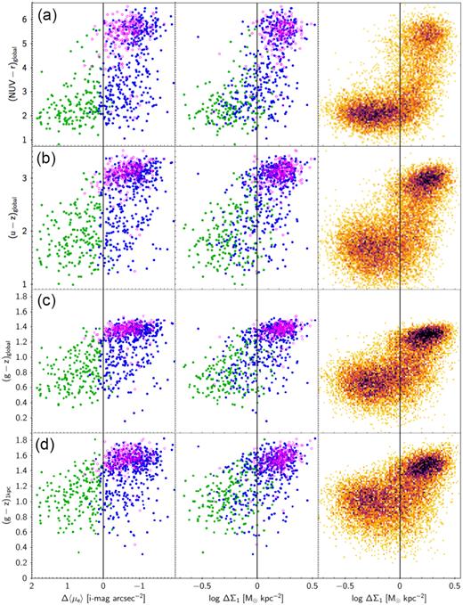
Four colours that are sensitive to star formation rate, stellar age, and dust content are plotted versus Δ〈μe〉 and ΔΣ1. Three are global, and the last is central. The format is the same as in Figs 10 and 11. All colours have been corrected for dust using the global estimates of Oh et al. (2011). The SDSS sample is smaller than the main sample by ∼1000 galaxies due to the extra requirement that spectroscopic S/N > 10. Inner 1 kpc colour (g − z)1kpc is computed from the surface brightness profile obtained from the SDSS data base (the colour g − z has been used since u is too noisy through a 1 kpc aperture). Note the elbow-shaped distributions in NUV − r and (to a lesser extent) in u − z. It is shown in the next panels that galaxies in the elbow have a high central density yet also a high star formation rate. These objects figure prominently in the discussion, and we have named them star-forming classical bulges (C-SFBs; see also Fig. 16).
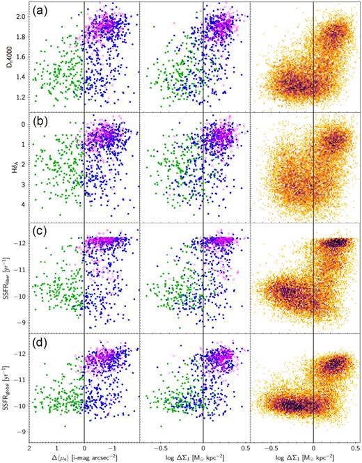
Three stellar-population indices from the SDSS spectra plus a fourth index showing global specific star formation rate from Brinchmann et al. (2004) are compared to Δ〈μe〉 and ΔΣ1. The format is the same as in Figs 10 and 11. The presence of the elbow in the first three panels confirms the presence of ongoing star formation and young stellar ages in the centres of star-forming classical bulges (C-SFBs). The fourth panel agrees with NUV − r in Fig. 12 and establishes that young stars are present throughout, not just in the inner parts. The downward trend from left to right for star-forming galaxies in panel (c) indicates even higher star formation rates at higher central densities.
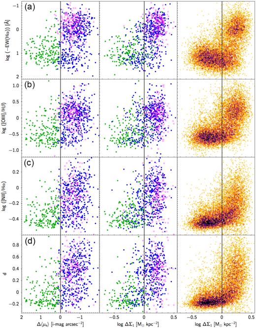
Four emission-line ratios compared to Δ〈μe〉 and ΔΣ1. The format is the same as in Figs 10 and 11. The H α equivalent width is multiplied by −1 and the y-axis is reversed to maintain the same sense as in other figures. (Taking logs loses roughly 2 per cent of galaxies, which have intrinsically positive EWs near zero.) The quantity d is the distance of a galaxy from the line dividing star-forming galaxies from AGNs according to Kauffmann et al. (2003c); its equation is given in the text. These emission-line data confirm the presence of ongoing star formation at the centres of star-forming classical bulges (C-SFBs), in agreement with the absorption indices and |$\rm SSFR_{\rm fibre}$| in Fig. 13. The downward tilt in EW(H α) signals higher ongoing star formation in elbow galaxies.
Fig. 12 shows four colour indices that are diagnostic of stellar age, star formation rate, and/or dust. The first three are global, and the last one is for the inner 1 kpc only.
12(a), NUV − r: This UV index is sensitive to ongoing star formation with an averaging time of a few tens of millions of years (e.g. Yesuf et al. 2014). The quenched clump at upper right is underpopulated because red galaxies tend to be missed in GALEX on account of their low UV flux. The main new feature in this plot is the pronounced ‘elbow’, which is visible in both the G09 and SDSS samples. The elbow was discovered previously in SDSS galaxies by Fang et al. (2013) using NUV − r versus ΔΣ1 and shown to exist out to z = 3 by Barro et al. (2017) using specific star formation rate instead of NUV − r (see also Mosleh et al. 2017; Lee et al. 2018).
We call attention to the dramatically different appearance of this panel from the previous panels in Figs 10–11, which used structural variables and were generally monotonic. The difference signals a divergence between structural properties and stellar-population properties, which will be repeated in all subsequent spectral parameters. Objects in the clump at upper right are quenched galaxies with high central density. Objects at lower left are star forming with a low central density. The objects in the elbow are aberrant in having high star formation rates despite having a high central density. We have named these objects star-forming classical bulges (C-SFBs), and their location is also highlighted in Fig. 16. These objects seem poised to enter the GV, and their properties may therefore provide a clue to the mechanics of quenching. The ridgeline of star-forming galaxies at the bottom of the distribution is also strikingly flat, suggesting no large trend in global specific star formation rate with central density as long as galaxies are star forming.
The preceding paragraph has defined a new subclass of C-bulges, but it is seen from the G09 plots in Fig. 12 that the exact membership in this class is not quite the same depending on whether C-bulges are defined using Δ〈μe〉 or ΔΣ1. While ΔΣ1 is preferred because it is used for the larger SDSS sample, we stress that the new subclass C-SFBs is basically just a useful name that calls attention to the fact that the relation between the structural variables and the stellar-population variables is highly non-linear, which is true regardless of whether ΔΣ1 or Δ〈μe〉 is used. The exact membership in this class is not important in what follows.
12(b), (u − z)global: The plot of (u − z)global resembles that of NUV − r but with lower dynamic range. The elbow is still present but is slightly less prominent. The quenched sequence at the top of the SDSS distribution is tilted slightly upward, suggesting an age gradient within the quenched population. Unlike NUV − r, the ridgeline of star-forming galaxies tilts slightly downwards towards higher ΔΣ1. Overall, these diagrams resemble plots of Sérsic index and/or concentration versus global (u − r) in Driver et al. (2006), Baldry et al. (2006), and Ball et al. (2008), which with the benefit of hindsight look rather elbow shaped.
The next two panels compare central versus global colours in the same colour index. Since u is too noisy through a 1 kpc aperture, g − z is used.
12(c), (g − z)global: The dynamic range of this colour index is less than NUV − r or u − z. The upward tilt of quenched galaxies that was seen in u − z remains visible, but the elbow looks weaker because the colour of the C-SFB population is quite red in this index. It appears that some C-SFB objects have moved up into the GV, or even merged with the quenched clump using this colour. The combination of red g − z plus blue NUV − r could mean dust (e.g. Williams et al. 2009; Brammer et al. 2011; Patel et al. 2011) or composite stellar populations (Wang et al. 2017). ΔΣ1 appears slightly tighter than Δ〈μe〉 in the G09 sample.
12(d), (g − z)1kpc: This g − z is measured within 1 kpc whereas the dust correction from Oh et al. (2011) is global, and so there is the possibility of mismatch. The total dynamic range is smaller than (g − z)global, which says that colour gradients are larger in star-forming galaxies than in quenched galaxies (centres are slightly redder). Whether this is due to older stars or more dust cannot be answered without more data.
The main result from Fig. 12 is to highlight evidence for a high-density star-forming population near the elbow of NUV − r and other colours, which we have termed the C-SFB population. Such a population was seen before in Fang et al. (2013), Barro et al. (2017), Woo et al. (2017), Mosleh et al. (2017), and Lee et al. (2018) using global indices. An attempt using g − z in Fig. 12(d) to see whether young stars also extend to the centres of these galaxies was inconclusive. Figs 13 and 14 will test this idea using central SDSS indices.
13(a), Dn4000: Dn4000 is a commonly used age indicator that averages star formation over time-scales of a few hundred million years (e.g. Yesuf et al. 2014). In Fig. 13(a), Δ〈μe〉 and ΔΣ1 scatter nearly equally in the G09 sample, and the C-SFB elbow is very strong in both, confirming that young central stars are present. Additional panels with other indices below confirm this. It is interesting to compare the large SDSS population in the right-hand panel with the corresponding panel for NUV − r in Fig. 12(a). The elbow is prominent in both, but Dn4000 actually declines with ΔΣ1 in star-forming galaxies, indicating even younger stars at the centres of C-SFB galaxies (the SDSS fibre spans approximately 1–4 kpc at these distances). This appears in subsequent figures and agrees with similar findings by Woo & Ellison (2019), who found younger stars in the centres of denser star-forming galaxies (see below). Kauffmann et al. (2003b) plotted Dn4000 versus effective stellar mass density, μ*, rather than ΔΣ1 as here. The same two clumps of star-forming and quenched galaxies were seen coexisting at a high density, but the decline in Dn4000 among the star-forming population was not apparent. This may be because they used absolute density, not a residual, for a sample that contained a wide range of stellar mass.
13(b), H δA: This index is corrected for emission and is a sensitive young-star indicator with a response time comparable to NUV − r (Yesuf et al. 2014). Δ〈μe〉 and ΔΣ1 both scatter broadly relative to H δA in the G09 sample. In SDSS, the quenched peak is strong and tight, but star-forming galaxies scatter widely. The latter effect hints at different central star formation histories even while galaxies are on the main sequence. Known processes that can cause H δA to differ from longer time-scale indices (like Dn4000) include starbursts and rapid quenching (e.g. Dressler & Gunn 1983; Zabludoff et al. 1996; Quintero et al. 2004; Yesuf et al. 2014). However, independent of scatter, the general star-forming population again tilts downward versus ΔΣ1, replicating Dn4000 and supporting the presence of relatively younger stars at the centres of C-SFBs. The large scatter in H δA in star-forming galaxies compared to Dn4000 and other central indices (see below) is another new finding and is not understood.
13(c), |$\rm SSFR_{\rm fibre}$|: This is the specific star formation rate within the fibre from Brinchmann et al. (2004). A major surprise is the very strong downward trend with ΔΣ1, signalling much larger SSFR in the centres at a high density and supporting and amplifying previous results from Dn4000 and H δA and from |$\rm SSFR_{\rm global}$| in the next panel.
13(d), |$\rm SSFR_{\rm global}$|: This is the specific star formation rate for the entire galaxy from Brinchmann et al. (2004). It combines the measurement of H α flux in the fibre with additional colour information from the outer parts. Its morphology generally matches that of the other global index, NUV − r in Fig. 12(a). The C-SFB population in the elbow is prominent, signalling strong ongoing global star formation, and the ridgeline is much more level than in Dn4000 or H δA and more like NUV − r.
In total, Figs 12 and 13 strongly establish the presence of young stars and ongoing star formation both globally and at the centres of C-SFB galaxies. The high star formation rates in these galaxies are therefore a general phenomenon not confined to the outer parts (i.e. we are not seeing dead, red bulges, and blue outer discs). There is evidence from Dn4000, H δA, and |$\rm SSFR_{\rm fibre}$| of even stronger star formation activity in the centres of C-SFB elbow galaxies than in the centres of low-Σ1 galaxies farther from the quenched ridgeline. This finding is consistent with the results of Woo & Ellison (2019), who study age and star formation rate gradients in star-forming SDSS galaxies as a function of ΔΣ1. Galaxies with high ΔΣ1 tend to have strong age gradients with younger stellar populations and higher specific star formation rates in their centres, while lower ΔΣ1 galaxies have older centres with lower specific star formation rates. Woo & Ellison (2019) study gradients whereas we study absolute central values, but the results are consistent.
Finally, Fig. 14 adds four more emission-line indices that shed further light on star formation and AGNs.
14(a), EW(H α): This index has not been corrected for dust, but we have verified that the basic morphology remains unchanged if the reddening corrections of Oh et al. (2011) are used (note that EWs here are multiplied by −1). The morphology is similar to Dn4000 in Fig. 13(a). Δ〈μe〉 and ΔΣ1 in the G09 sample look similar, and both exhibit a strong elbow, as does SDSS. The quenched clump in SDSS is broadened due to the presence of Seyfert and LINER emission, which varies from galaxy to galaxy. The downward tilt along the horizontal branch duplicates similar trends in Dn4000, H δA, and |$\rm SSFR_{\rm fibre}$|, but the very short time-scale of H α directly implies higher ongoing star formation in elbow galaxies, not just younger average age.
14(b), [O iii]/H β: This is one of two line ratios used to divide star-forming galaxies and AGNs in the BPT diagram. Δ〈μe〉 and ΔΣ1 in the G09 sample look similar, and both exhibit a strong elbow in the C-SFB population, which is also seen in the SDSS sample. The ratio is flat at the star-forming value into the elbow, indicating ongoing star formation there, shifting to the AGN value for galaxies in the quenched clump.
14(c), [N ii]/H α: This is the other line ratio used to divide star-forming galaxies from AGNs in the BPT diagram. The plots resemble [O iii]/H β except that [N ii]/H α scatters more widely in quenched galaxies, and [N ii] appears to increase faster than [O iii] as galaxies evolve into the GV.
14(d), d: The quantity d is the slanting distance of a galaxy from the dividing line between star-forming and AGN galaxies in the BPT diagram defined by Kauffmann et al. (2003c) and is computed as d = log ([O iii]/H β) − 0.61/[log ([N ii]/H α) − 0.05] − 1.3. The diagram looks like an average of [O iii]/H β and [N ii]/H α, as expected.
We now summarize the major conclusions from Figs 10–14. We stress again that the SDSS sample is for central galaxies only with log M*/M⊙ > 10.0 and the behaviour of satellites may be different (Woo et al. 2017).
First, Δ〈μe〉 and ΔΣ1 appear to characterize the structural state of bulges similarly in that both measure bulge prominence via central density. Although the left-hand and middle panels of these figures differ in detail, they are broadly similar. Since Δ〈μe〉 is one of the standard parameters used to classify P-bulges and C-bulges (e.g. G09; FD16), it follows that ΔΣ1 is also a serviceable indicator of bulge structure, with the additional advantages that it does not require bulge–disc decomposition and it can be measured out to z = 0.07 in SDSS images (Fang et al. 2013) and out to z = 3 in HST images (Barro et al. 2017). We have therefore met one of the major goals of this paper, to compare ΔΣ1 to at least one other classical bulge structure indicator, and we have shown that it compares favourably and measures similar bulge properties. We also note that ΔΣ1 has had the mass trend removed, and therefore for consistency other mass-dependent parameters should also have their mass trends removed before comparing to it.
Secondly, the different panels of Figs 10–14 exhibit a wide variety of different morphologies that suggest a wealth of information yet to be unlocked with additional analysis. This is reinforced by the discovery, to be discussed in future papers, that the broad, fuzzy loci in Figs 10–14 are actually comprised of subpopulations in different evolutionary stages. This is the reason we have warned against overinterpreting the entire ridgelines as evolutionary tracks. Instead, it is the various subpopulations within these patterns that are the tracks, as will be shown in future papers.
Thirdly, the locus of star-forming galaxies is rather flat versus ΔΣ1 using global parameters like NUV − r, u − z, and |$\rm SSFR_{\rm global}$| but it trends downward at high Σ1 using central parameters like Dn4000, H δ, EW(H α), and |$\rm SSFR_{\rm fibre}$|.7 This shows conclusively that not only is global star formation high in C-SFB elbow galaxies but also central star formation is even higher. This finding of younger stars and higher star formation at the centres of high-density C-SFBs agrees with measurements of stellar-population gradients by Woo & Ellison (2019).
The final point, mentioned above, is that correlations involving purely structural parameters (including Δ〈μe〉 and ΔΣ1) seem to be rather straight in log–log space whereas correlations that mix stellar-population variables with Δ〈μe〉 and ΔΣ1 are elbow shaped. We have verified separately that the elbow objects are substantially the same in all diagrams. Together, these results suggest that central galaxies in this mass range possess a well-correlated set of structural parameters and a separate set of well-correlated stellar-population parameters and that elbow relations result when mixing parameters from the two classes.
7 DISCUSSION
7.1 Comparison to previously measured bulge types
Our most important finding is that star formation rates do not correlate perfectly with central structure – galaxies with ΔΣ1 < 0 are all star forming, whereas galaxies with ΔΣ1 > 0 are a mixture of quenched and star-forming galaxies (the ‘elbow’ pattern). This pattern persists even when even more global structural parameters, such as concentration, B/T, nglobal, and re, are used. Finally, different indices are quite consistent: All structural parameters show roughly linear relations against ΔΣ1, whereas all star-forming indices show elbows.
As shown in the left-hand and middle panels of Figs 10–14, these results agree very well with G09, as might be expected since our ΔΣ1 bulge calibration is closely modelled on his parameter Δ〈μe〉. However, the bulge-type literature in general has used a much wider range of bulge-classification parameters, and to compare to them, we use the summary of correlations by FD16. Several conclusions are at variance with the very clear trends in Figs 10–14. Broadly speaking, sources agree that the majority of P-bulges are low density and high star forming and that the majority of C-bulges are high density and low star forming, but difficulties arise when trying to make sense of the outliers.
To illustrate, we select four findings from FD16 and add some comments. We primarily rely on the SDSS sample but refer occasionally to the G09 sample when needed.
‘Though C-bulges are rarely found to be blue, P-bulges are often red’. Neither of these conclusions agrees with our data. If C-bulges are defined as galaxies that lie to the right of the vertical lines in Figs 10–14, it is seen that a substantial portion of them are blue and star forming. More quantitatively, using the mass-limited SDSS sample and setting aside the 642 elliptical galaxies leaves 5588 C-bulges. Dividing them at Dn4000 = 1.6 gives 3238 red galaxies and 2350 blue galaxies. Thus, 42 per cent of central C-bulges in the mass range 10.0 < log M*/M⊙ < 10.4 are blue. It is likely that this fraction varies with mass and environment: More massive galaxies are redder and more quenched than the SDSS sample (e.g. Baldry et al. 2006; Ball et al. 2008), and including satellites would also add more red galaxies. Nevertheless, the fraction of 42 per cent in our sample does not really merit the word ‘rare’.
The second part of the sentence also does not agree, as P-bulges in the SDSS sample are virtually never red. Again, the statement may be sample dependent, as low-ΔΣ1 galaxies are redder when they are satellites (Woo et al. 2017) and also when they are massive (Ball et al. 2008). Both satellites and massive galaxies have been pruned from the SDSS sample but not from the G09 sample, and more red P-bulges may indeed be present there. The tentative conclusion is that the detailed distributions of galaxies in these diagrams may depend on both mass and environment (cf. Ball et al. 2008) and that general conclusions should be carefully qualified.
‘If a bulge is star forming (and there is no interaction present), this is very good evidence that the bulge is a pseudo-bulge, but when the bulge is not star forming this does not imply that the bulge is classical’. Again, both of these conclusions disagree with our data. In the SDSS sample, 29 per cent of star-forming bulges are C-bulges in this mass range, which means that the P-bulge prediction would be wrong nearly one-third of the time, not really a ‘very good’ prediction. As for non-star-forming bulges, virtually all are classical in the SDSS sample, contrary to FD16. However, the number of P-bulges among red galaxies would be increased by including satellites, so the environmental dependence of the distributions may again be an issue.
‘Though P-bulges are rarely found to have high σ, C-bulges may have either high or low σ’. This statement generally agrees with our data, especially if one imagines adding more massive galaxies to the SDSS sample in Fig. 11(a). However, we have argued that use of a mass-corrected residual Δσ1 is more appropriate than the use of an absolute σ1.
‘Bulges that consist of both a thin, star-forming pseudo-bulge and a hot-passive classical bulge are very likely present in some galaxies’. This statement is made in the context of so-called composite bulges, which are objects that exhibit properties of both bulge types (e.g. Erwin et al. 2015). Such objects might be an intriguing way to account for the properties of C-SFBs, i.e. elbow galaxies that have high central density yet high central star formation. However, we have checked this possibility using the sample of composite bulges in Erwin et al. (2015) and find that few of them actually host active central star formation (they are mostly S0’s). Moreover, the elbow phenomenon strongly exists in NUV − r as well as the SDSS indices (Fig. 12a), and NUV − r, being global, would not be much affected by star formation in a pseudo-bulge. It thus appears that the division between active and passive C-bulges is a global phenomenon, not one that is associated with the presence or not of a composite bulge.
The previous bullets have highlighted instances of disagreements between this paper and the findings in FD16. However, the problem of classifying bulges is more general and has been noted in several works (e.g. G09; K16). On reflection, we think that most disagreements in classifying individual galaxies can be chalked up to four causes: a certain amount of noisy data, reliance on hard-to-measure and possibly inconclusive quantities like nbulge, failure to use mass-corrected residual quantities consistently, and failure to recognize the fundamentally non-linear (elbow-shaped) relation between structure and stellar populations, which give discrepant classifications for elbow galaxies. Discrepancies in broader trends may arise from these effects as well as differences in the mass ranges and environmental densities used. We hope to explore these second-parameter effects in future papers.
7.2 Frequency of bulge types versus stellar mass
Another comparison to previous work is the frequency of bulge types as a function of stellar mass. Fig. 15 repeats this plot from Fisher & Drory (2011) with our SDSS data added. The lower limit is set to log M*/M⊙ = 9.5, as SDSS magnitude incompleteness corrections are large below that. No correction is made for fibre targeting incompleteness (Section 2), but if this is a function of apparent magnitude only, then the resulting distributions are at least relatively correct. For bulge types, we use the three populated quadrants shown in Fig. 16: (1) lower left, P-bulges (ΔΣ1 < 0); (2) lower right, star-forming C-bulges (C-SFBs); and (3) upper right, quenched C-bulges (C-QBs). Ellipticals are included as a fourth category in the upper panel of Fig. 15 using P(Ell) > 0.65 from Huertas-Company et al. (2011) (see Section 2) but they are not included in the lower panel. We cannot distinguish between N-bulges and P-bulges, and so our P-bulge category lumps them together.
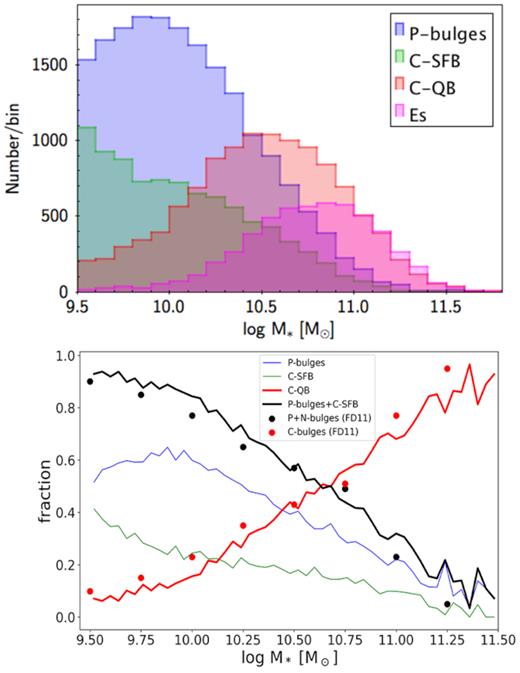
Top panel: The number of SDSS galaxies of different bulge types in 0.2 dex mass bins. P-bulges are defined as galaxies in the lower left quadrant of Fig. 16, C-SFBs are the star-forming C-bulges in the lower right quadrant, and C-QBs are quenched galaxies in the upper right quadrant (E’s included). Magnitude incompleteness corrections are applied to all numbers. Bottom panel: Fractions of various bulge types versus mass, with ellipticals now excluded. The black and red dots are analogous data from Fisher & Drory (2011). Good agreement is achieved if it is assumed that the FD P-bulges comprise mostly star-forming bulges while their C-bulges are mostly quenched, i.e. that their bulge-typing criteria weight stellar-population properties more than central density.
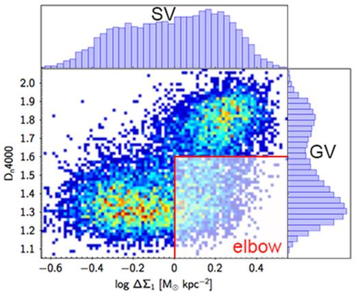
Dn4000 versus ΔΣ1 and their histograms for our mass-limited SDSS sample of central galaxies in the range 10.0 < log M*/M⊙ < 10.4. Points are colour coded by the number density weighted by the magnitude completeness correction. The dip in the Dn4000 histogram is the familiar GV. The dip in the ΔΣ1 histogram is the SV (cf. Figs 1, 5, and 6). Even though each axis shows two peaks, the makeup of the peaks is not the same because of the existence of the galaxies at the elbow (shaded region to lower right). Elbow galaxies are spectrally P-bulges but structurally C-bulges, which demonstrates the different nature of the GV and SV – they are not defined by the same objects.
The top panel of Fig. 15 shows the number of galaxies per 0.2 dex mass bin. As expected, mass trends are strong, with P-bulges concentrated at lower masses, C-QBs at intermediate masses, and ellipticals at high masses. Somewhat unexpected is the similarity of the C-SFB bulges to P-bulges. One might have expected them to be intermediate between P-bulges and C-QBs, but they are very close to P-bulges, suggesting a close evolutionary connection.
The bottom panel shows fractions of the three bulge types (minus ellipticals) versus mass. The black and red dots show analogous data points from Fisher & Drory (2011). The black points are for the galaxies they call P+N-bulges, and the red dots are for the galaxies they call C-bulges. Interestingly, good agreement is achieved if their P-bulges are identified with our P+C-SFBs and their C-bulges are identified with our C-QBs. A hypothesis is that the net criteria used by FD16 weight stellar-population-related properties more heavily than central density. That would mean assigning types by cutting Fig. 16 horizontally through the GV rather than vertically through the SV. We notice that no matter which criteria we choose to identify P-bulges, there are still many massive P-bulges (more than 20 per cent at log M*/M⊙ = 11.0). Given that P-bulges may be converted to C-bulges via mergers, previous authors (e.g. Kormendy et al. 2010) have highlighted the continued existence of these galaxies. We reinforce this problem here, and Chen et al. (2019) may help explain this from a theoretical point of view.
7.3 Are bulge properties bimodal?
We turn now to the topic of ‘bimodality’, which might potentially play an important role in deducing the origins and evolution of bulges. Much of the literature on bulge types claims that P-bulges and C-bulges are ‘bimodal’, which according to the strict definition of the word means a population showing two separate peaks. A search of the literature reveals only one structural parameter histogram that is convincingly bimodal, a histogram of nbulge that shows two peaks in Fisher & Drory (2010). However, as the authors say, the sample in that paper is overweighted by Virgo Cluster galaxies, which might tend to produce a false peak at high nbulge. In fact, a later version of this histogram with more galaxies does not display two separate peaks but rather one smooth (if noisy) distribution (FD16). P-bulges are clustered at one end, and C-bulges are clustered at the other, but there is no strong feature in the histogram itself that signals two distinct populations.
Three points are relevant. First, it is necessary to employ large and representative samples when testing histograms for bimodality – overweighting the Virgo Cluster may create a false peak where none exists. Secondly, the fact that a second parameter varies systematically from one end of a distribution to the other does not mean that the base population is bimodal; it merely says that two variables are correlated. Thirdly, genuine bimodality would be significant because it might signal that P-bulges and C-bulges are formed by separate mechanisms. In fact, as noted in the ‘Introduction’ section, it is a common view that P-bulges are formed by secular evolution while C-bulges are formed by mergers (or perhaps by violent disc instabilities when galaxies were young and gas rich) (e.g. FD16; K16). The existence of two clearly separate peaks in any property might therefore support this picture.
An important insight from Figs 12–14 is that bimodality for bulges should properly be considered simultaneously in both spectral and structural space. No single histogram, whether it uses a structural variable or a spectral variable, can convey the full 2D parameter distribution of these objects. This is illustrated in Fig. 16, which replots Dn4000 versus ΔΣ1 for SDSS central galaxies with masses in the range 10.0 < log M*/M⊙ < 10.4. Histograms of the distributions in ΔΣ1 and Dn4000 are on the X- and Y-axes. It is true that both histograms are bimodal. The Dn4000 distribution shows the well-known dichotomy between star-forming and quenched galaxies, separated by the GV. The ΔΣ1 histogram is also (weakly) bimodal. This is the same feature that was highlighted in Figs 5 and 6, which we dubbed the SV.8 However, these histograms in X and Y are not the most effective way to demonstrate the true bimodality of the population – that is most clearly shown by the two islands in two dimensions, and thus the bimodality in question is neither purely structural nor purely spectral but a combination of the two. The final point is that the objects that comprise the two peaks in Dn4000 are not exactly the same as the objects that comprise the two peaks in ΔΣ1. That is because the elbow galaxies (shaded region) are members of the P-bulge peak based on star formation rate, but they are members of the C-bulge peak based on structure. Hence, a one-dimensional classification system using only structural data, as we have employed here, will necessarily give an incomplete and confusing picture – the population needs to be modelled in both spectral and structural space simultaneously for a full understanding.
These conclusions were already evident from plots that mixed structural variables and spectral variables in Kauffmann et al. (2003b), Driver et al. (2006), Baldry et al. (2006), and Bell (2008), but they are now clearer using the larger array of spectral indices and the mapping on to structural bulge types in Figs 12–14.
7.4 Bulge types in relation to galaxy quenching
A final point is the close connection between the results here to previous papers on Σ1 in galaxies. It is now clear that the ‘elbow’ seen in Figs 12–14 is the same elbow pattern in SDSS galaxies seen by Fang et al. (2013) in which galaxies with low ΔΣ1 have high star formation but galaxies with high ΔΣ1 have a wide range of star formation rates. Barro et al. (2017) and Lee et al. (2018) showed that this elbow pattern is ancient and extends back to at least z = 3 in CANDELS. It is thus a deeply ingrained feature of how (central) galaxies fade in our Universe. A major result of this work is to show how bulge types – P-bulges, C-bulges, and E’s – map on to this pattern. If the local mapping is universal, distant galaxies would also exhibit P-bulge and C-bulge properties similar to nearby galaxies. If our picture that galaxies are evolving from low ΔΣ1 to high ΔΣ1 today is correct, it would follow that the entire sequence from N-bulge to P-bulge, C-bulge, and finally to E’s is an evolutionary progression that exists at all redshifts.
Fang et al. (2013) attempted to explain the non-linear correlation between star formation rate and ΔΣ1 in terms of quenching by black hole feedback. Their picture was motivated by the relations MBH ∼ σ4 and |$\Sigma _1 \sim \sigma _1^2$|, the latter also measured by Fang et al. (2013). Thus, |$M_{BH} \sim \Sigma _1^2$|, and central density Σ1 becomes an indicator of BH mass. According to this picture, galaxies build bulges and black holes together before they quench. C-SFBs in the elbow are star-forming galaxies at the tipping point, while C-bulges on the vertical branch are former C-SFBs in which BH feedback is finally having a measurable dampening effect on star formation rate. In other words, the elbow-shaped distributions are due to the fact that structure and stellar populations evolve differently near quenching. Remaining questions are why galaxies tend to quench at a particular mass and why the quenched ridgeline in Σ1 versus M* has the observed slope and zero-point (Fig. 1a). These topics are addressed in a companion paper to this one on how black holes might quench galaxies by transferring energy to the hot gas in their dark haloes (Chen et al. 2019).
8 CONCLUSIONS
In this paper, we study the relationship between the stellar mass surface density within 1 kpc, Σ1, and the nature of galactic bulges in SDSS galaxies with 0.02 < z < 0.07 and log M*/M⊙ > 10.0. The goals are to establish how Σ1 relates to other bulge-classification parameters and to see if it can be used to identify C-bulges and P-bulges in SDSS. A residual parameter ΔΣ1 is defined by removing the mass trend from Σ1. Since ΔΣ1 can be measured from SDSS aperture photometry without the need for delicate bulge–disc decompositions, success in using ΔΣ1 would open the SDSS sample out to z = 0.07 to further bulge studies.
A sample of nearly 1000 SDSS galaxies from Gadotti (2009) with careful bulge–disc–bar decompositions and measured values of the established bulge-classification parameter Δ〈μe〉 is used to validate ΔΣ1. ΔΣ1 is compared to Δ〈μe〉 for the G09 sample and also to a larger mass-limited sample of SDSS central galaxies in the range 10.0 < log M*/M⊙ < 10.4. Results are as follows:
ΔΣ1 and Δ〈μe〉 (from G09) measure similar aspects of bulge structure, and derived bulge types, both P-bulge and C-bulge, are broadly similar. ΔΣ1 can be used to provide statistically useful measures of bulge types for SDSS galaxies out to z = 0.07.
According to either ΔΣ1 or Δ〈μe〉, the main distinction between bulge types is central stellar density: P-bulges have low central densities, while C-bulges have high central densities.
Additional SDSS parameters are compared to ΔΣ1 and Δ〈μe〉. Structural parameters (based on kinematics and mass-density profiles) show fairly linear log–log relations versus Δ〈μe〉 and ΔΣ1 with only moderate scatter. Stellar-population parameters in contrast show a highly non-linear ‘elbow’ in which specific star formation rate remains roughly flat with central density and then falls rapidly at the elbow, where galaxies begin to quench. Similar trends are seen for both central and global star formation indicators. The elbow seen here is the same as the feature seen by Fang et al. (2013) for SDSS galaxies and by Barro et al. (2017), Mosleh et al. (2017), and Lee et al. (2018) for CANDELS galaxies.
In the mass-limited central SDSS sample, P-bulges are found to be a homogeneous class, are universally star forming, and occupy the low-density portion of the horizontal elbow arm. C-bulges in contrast exhibit a wide range of star formation rates from quenched to highly active and occupy the elbow itself and the vertical branch above it. New terminology is introduced to subdivide C-bulges according to star formation rate: C-SFBs are star-forming C-bulges in and near the elbow, while C-QBs are quenched C-bulges at the end of the vertical branch. Preliminary evidence is mentioned that the detailed distributions of galaxies along and off the elbow may also vary with mass and environment.
Classifying galaxies as P-bulges or as C-bulges has been difficult in the past because criteria sometimes disagree. Results here suggest that a major reason is the elbow-shaped correlations between structural parameters and star formation indices, which means that classifying objects by structure as opposed to stellar-population indices will disagree for many galaxies.
Bimodality in bulge types has been discussed in the bulge-classification literature. A major conclusion from this work is that distributions in spectral and structural parameters are both bimodal, stemming from the existence of two distinct ‘islands’ that are clearly visible in plots of spectral versus structural parameters. Understanding the bimodality of bulges will thus require modelling structure and stellar populations simultaneously.
The structural and stellar-population relationships in this paper and their variation from index to index suggest an unsuspected richness in the central properties of galaxies as their star formation rates begin to fade. Exploring these in future may shed light on how galaxies quench. Galaxies with IFU data from surveys such as the SDSS-IV MaNGA may be useful in providing spatially resolved star formation maps to further understand the evolution track. If evolution is really along the horizontal branch of the elbow and then upwards to quenching, what is the expected signature in star formation maps?
SUPPORTING INFORMATION
Table B1. Sample entries from the Σ1 catalogue for SDSS DR7 galaxies.
Please note: Oxford University Press is not responsible for the content or functionality of any supporting materials supplied by the authors. Any queries (other than missing material) should be directed to the corresponding author for the article.
ACKNOWLEDGEMENTS
We acknowledge financial support from NSF grants AST-0808133 and AST-1615730. YL acknowledges support from the China Scholarship Council. This work is also partly supported by the National Key Basic Research and Development Program of China (No. 2018YFA0404501) and by the National Science Foundation of China (Grant Nos. 11821303, 11333003, 11390372, and 11761131004 for SM and YL). ARP acknowledges partial support from UNAM PAPIIT grant IA104118, the CONACYT ‘Ciencia Basica’ grant 285721, the UC MEXUS postdoctoral fellowship, and UC MEXUS Collaborative Research Grant CN-17-125.
Funding for the SDSS and SDSS-II has been provided by the Alfred P. Sloan Foundation, the Participating Institutions, the National Science Foundation, the U.S. Department of Energy, the National Aeronautics and Space Administration, the Japanese Monbukagakusho, the Max Planck Society, and the Higher Education Funding Council for England. The SDSS website is http://www.sdss.org/.
GALEX (Galaxy Evolution Explorer) was a NASA Small Explorer, launched in 2003 April. We gratefully acknowledge the NASA’s support for construction, operation, and science analysis for the GALEX mission, developed in cooperation with the Centre National d’Études Spatiales of France and the Korean Ministry of Science and Technology.
We thank the referee for a thorough and stimulating referee report, which greatly improved the presentation. We also acknowledge our debt to Dmitri Gadotti for publishing his catalogue of μe and other bulge–disc decomposition parameters, which provided the calibration sample needed for understanding the larger SDSS sample.
Footnotes
The Σ1 value for SDSS DR7 galaxies is available online as supplementary material.
Note that G09 does not provide the mean effective surface brightness within the bulge effective radius 〈μe〉 in the online catalogue, but rather effective surface brightness at the bulge effective radius μe only. Thus, we compute 〈μe〉 ourselves using μe and bulge Sérsic index from the online catalogue.
As mentioned in Section 2 describing the sample, a signal-to-noise cut of S/N > 10 per pixel was applied in choosing the spectroscopic subsample, which caused the loss of about 1000 additional galaxies out of 12 000 (see Table 1). We have verified that these galaxies are mostly lost because they are dim, but they are otherwise relatively uniformly distributed as a function of ΔΣ1 and colour in Figs 12–14. Their loss does not therefore substantially distort the sample. No additional cuts are applied for emission-line S/N.
We have verified that this effect is not due to a fibre aperture effect by seeing no redshift dependence in any plot.
The bimodality is weaker here than that in Fig. 6 because the mass range here is log M*/M⊙ = 10.0–10.4 inclusive.
REFERENCES
APPENDIX A: REDDENING CORRECTIONS
A concern is how reddening corrections may have affected the distributions of galaxies in Figs 10–14. The reddening corrections of Oh et al. (2011) have been adopted here for colours (but not emission lines). Fig. A1 plots their E(B − V) versus ΔΣ1. These are global estimates for only the stellar continua. The mass range is limited to 10.0 < log M*/M⊙ < 10.4, and the Y-axis is inverted to match the sense of Figs 10–14. The striking elbow-shaped pattern in Fig. A1 matches the similar pattern in Figs 12–14, which also plots spectral parameters. The horizontal bottom branch contains star-forming galaxies, and the vertical branch is populated by fading and quenched galaxies, which in this figure have less or zero reddening.
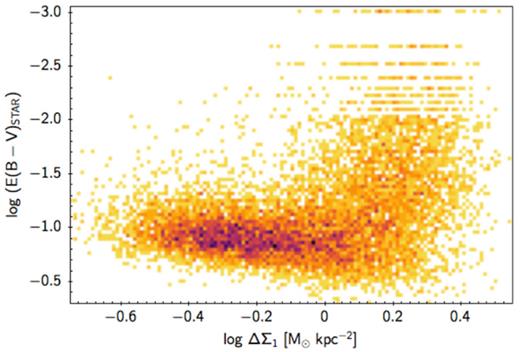
Reddening values for SDSS DR7 galaxies from Oh et al. (2011) plotted versus the bulge density parameter ΔΣ1. The sample used is the mass-limited SDSS sample in the mass range 10.0 < log M*/M⊙ < 10.4 used in Figs 10–14. Reddening values are global and are estimated for the stellar continuum. The Y-axis has been reversed to match the sense of Figs 10–14. The elbow pattern seen here matches similar patterns in Figs 12–14: The horizontal arm is populated by star-forming galaxies, and the vertical branch is populated by fading and quenched galaxies. Reddening is moderate overall and does not vary greatly along the star-forming branch across the bottom; average values range from only 0.10 to 0.17 mag. Conclusions from Figs 12–14 should therefore not depend sensitively on whether reddening corrections are applied or not.
The important features of the figure are the overall small values of E(B − V) and the small slope of the trend along the horizontal star-forming branch: Values of E(B − V) vary from 0.10 mag on average at low ΔΣ1 to about 0.17 mag on average at high ΔΣ1. Thus, E(B − V) is small on average and rather constant, even for star-forming galaxies. In the main text, we are interested in how star-forming indicators vary versus ΔΣ1 along this lower branch. The conclusion from Fig. A1 is that our results should not depend greatly on whether raw or reddening-corrected parameters are used, and this was confirmed by separate tests. Thus, we elect to use the reddening-corrected values of Oh et al. (2011) for all magnitudes and colours but use uncorrected values from SDSS DR7 for emission lines and spectral indices.
APPENDIX B: SUPPLEMENTARY DATA
The Σ1 value for SDSS DR7 galaxies with their SDSS identification can be found in the online version of this article. Notice that we only provide the Σ1 value for galaxies with 0.02 < z < 0.07 and axial ratio b/a > 0.5 to avoid the seeing degradation and the added opacity in edge-on galaxies.
Sample entries from the Σ1 catalogue for SDSS DR7 galaxies. The full table is available online as supplementary data.
| RA | DEC | SDSS DR7 objid | log Σ1 |
|---|---|---|---|
| 147.3295 | 0.0289 | 587725074995609782 | 9.4297 |
| 146.5128 | −0.8458 | 588848898824274111 | 9.4704 |
| 146.8644 | −0.4641 | 588848899361276123 | 9.0138 |
| 146.7559 | −0.1682 | 588848899898147178 | 8.2839 |
| 146.0937 | −0.7931 | 587725073921343655 | 9.7409 |
Note. The first three columns show the SDSS identification of the galaxies. Column (4) shows the log Σ1 value.
