


ABSTRACT
A new upper limit on the 21 cm signal power spectrum at a redshift of z ≈ 9.1 is presented, based on 141 h of data obtained with the Low-Frequency Array (LOFAR). The analysis includes significant improvements in spectrally smooth gain-calibration, Gaussian Process Regression (GPR) foreground mitigation and optimally weighted power spectrum inference. Previously seen ‘excess power’ due to spectral structure in the gain solutions has markedly reduced but some excess power still remains with a spectral correlation distinct from thermal noise. This excess has a spectral coherence scale of 0.25–0.45 MHz and is partially correlated between nights, especially in the foreground wedge region. The correlation is stronger between nights covering similar local sidereal times. A best 2-σ upper limit of |$\Delta ^2_{21} \lt (73)^2\, \mathrm{mK^2}$| at |$k = 0.075\, \mathrm{h\, cMpc^{-1}}$| is found, an improvement by a factor ≈8 in power compared to the previously reported upper limit. The remaining excess power could be due to residual foreground emission from sources or diffuse emission far away from the phase centre, polarization leakage, chromatic calibration errors, ionosphere, or low-level radiofrequency interference. We discuss future improvements to the signal processing chain that can further reduce or even eliminate these causes of excess power.
1 INTRODUCTION
Exploring the Cosmic Dawn (CD) and the subsequent Epoch of Reionization (EoR), comprising two eras from z ∼ 6−30 when the first stars, galaxies and black holes heated and ionized the Universe, is of great importance to our understanding of the nature of these first radiating sources. It provides insight on the timing and mechanisms of their formation, as well as the impact on the physics of the interstellar medium (ISM) and intergalactic medium (IGM) of the radiation emitted by these first light sources (see e.g. Ciardi & Ferrara 2005; Morales & Wyithe 2010; Pritchard & Loeb 2012; Furlanetto 2016, for extensive reviews).
Observations of the Gunn–Peterson trough in high-redshift quasar spectra (e.g. Becker et al. 2001; Fan et al. 2006) and the measurement of the optical depth to Thomson scattering of the Cosmic Microwave Background (CMB) radiation (e.g. Planck Collaboration XIII 2016b) both suggest that the bulk of reionization took place in the redshift range 6 ≲ z ≲ 10. The evolution of the observed Ly α Emitter (LAE) luminosity function at z > 6 (Clément et al. 2012; Schenker et al. 2013) and the Ly α absorption profile towards very distant quasars (Mortlock 2016; Greig et al. 2017; Davies et al. 2018) are other indirect probes of the EoR.
The most direct probe of this epoch, however, is the redshifted 21 cm line from neutral hydrogen, seen in emission or absorption against the CMB (Madau, Meiksin & Rees 1997; Shaver et al. 1999; Tozzi et al. 2000; Zaroubi 2013). A number of observational programs are currently underway, or have recently been completed that aimed to detect the 21 cm brightness temperature from the EoR and CD. The 21 cm global experiments, such as EDGES1 (Bowman et al. 2018) or SARAS2 (Singh et al. 2017) aim to measure the sky-averaged spectrum of the 21 cm signal. The tentative detection of the global 21 cm signal reported by the EDGES team (Bowman et al. 2018) has unexpected properties. This signal, consisting of a flat-bottomed deep absorption-line feature during the CD at z = 14−21, is considerably stronger and wider than predicted (Fraser et al. 2018), and, depending on the additional mechanism invoked to explain it (e.g. Barkana et al. 2018; Berlin et al. 2018; Ewall-Wice et al. 2018; Fialkov & Barkana 2019; Mirocha & Furlanetto 2019), could also have an impact on the predicted strength of the 21 cm brightness temperature fluctuations during the EoR. Complementary to these, the interferometric experiments aim at a statistical detection of the fluctuations from the EoR using radio interferometers such as LOFAR,3 MWA,4 or PAPER.5
These instruments have already set impressive upper limits on the 21 cm signal power spectra, considering the extreme challenges they face, but have not yet achieved a detection. Using the GMRT,6 Paciga et al. (2013) reported a 2 − σ upper limit of |$\Delta _{21}^2 \lt (248\, \mathrm{mK})^2$| at z = 8.6 and wavenumber |$k \approx 0.5 \,\mathrm{h\, cMpc^{-1}}$| from a total of about 40 h of observed data. Recently, Barry et al. (2019) reported a 2 − σ upper limit of |$\Delta _{21}^2 \lt (62.4\, \mathrm{mK})^2$| at z = 7 and |$k \approx 0.2 \,\mathrm{h\, cMpc^{-1}}$| using 21 h of Phase I MWA data, and Li et al. (2019) published a 2 − σ upper limit of |$\Delta _{21}^2 \,\lt (49\, \mathrm{mK})^2$| at z = 6.5 and |$k \approx 0.59\, \mathrm{h\, cMpc^{-1}}$| using 40 h of Phase II MWA data. The PAPER collaboration reported a very deep upper limit (Ali et al. 2015), but after re-analysis (Cheng et al. 2018) have recently reported revised and higher upper limits (Kolopanis et al. 2019), the deepest being |$\Delta _{21}^2 \lt (200\, \mathrm{mK})^2$| at z = 8.37 and |$k \approx 0.37\, \mathrm{h\, cMpc^{-1}}$|. In Patil et al. (2017), the LOFAR-EoR Key Science Project (KSP) published their first upper limit based on 13 h of data from LOFAR, reporting a 2 − σ upper limit of |$\Delta _{21}^2 \lt (79.6 \,\mathrm{mK})^2$| at z = 10.1 and |$k \approx 0.053 \,\mathrm{h\, cMpc^{-1}}$|.
Much more research is still needed, however, to control the many complex aspects in the signal processing chain (Liu & Shaw 2019) in order to reach the expected 21 cm signal strengths which lie two to three orders of magnitude below these limits (e.g. Mesinger, Furlanetto & Cen 2011). Mitigating all possible effects that could prevent a 21 cm signal detection is particularly important since these instruments are also pathfinders for the much more sensitive and ambitious second-generation instruments such as the SKA7 (Koopmans et al. 2015) and HERA8 (DeBoer et al. 2017).
At the low radiofrequencies targeted by 21 cm signal observations, the radiation from the Milky Way and other extragalactic sources dominates the sky by many orders of magnitude in brightness (Shaver et al. 1999). The emission of these foregrounds varies smoothly with frequency, and this characteristic can be used to differentiate it from the rapidly fluctuating 21 cm signal (Jelić et al. 2008). However, due to the ionosphere and the frequency-dependent response of the radio telescopes (e.g. its primary beam and uv-coverage both scale with frequency), structure is introduced to the otherwise spectrally smooth foregrounds, causing the so-called ‘mode-mixing’ (Morales et al. 2012). Most of these chromatic effects are confined inside a wedge-like shape in k-space (Datta, Bowman & Carilli 2010; Trott, Wayth & Tingay 2012; Vedantham, Udaya Shankar & Subrahmanyan 2012; Liu, Parsons & Trott 2014a,b), and to mitigate them, many experiments adopt a ‘foreground avoidance’ strategy which only performs statistical analyses of the 21 cm signal inside a region in k-space where the thermal noise and 21 cm signals dominate (e.g. Jacobs et al. 2016; Kolopanis et al. 2019). In practice, however, leakage above the wedge is also observed and is thought to be due to gain-calibration errors because of an incomplete or incorrect sky model (Patil et al. 2016; Ewall-Wice et al. 2017), errors in band-pass calibration, cable reflections (Beardsley et al. 2016), multipath propagation, mutual coupling (Kern et al. 2019), residual radiofrequency interference (RFI) (Offringa, Mertens & Koopmans 2019a; Whitler, Beardsley & Jacobs 2019), as well as chromatic errors introduced due to leakage from the polarized sky into Stokes I (Jelić et al. 2010; Spinelli, Bernardi & Santos 2018) or ionospheric disturbances (Koopmans 2010; Vedantham & Koopmans 2016).
By modelling and removing the foreground contaminants, the LOFAR EoR KSP team aims at probing the 21 cm signal both outside and inside the wedge, thereby potentially increasing the sensitivity to the 21 cm signal by an order of magnitude (Pober et al. 2014) and enabling exploration of the signal at the largest available scales, which have more significance for cosmology/signal-clustering studies. This has required the development of a comprehensive sky model of the North Celestial Pole (NCP) field (Yatawatta et al. 2013; Patil et al. 2017), currently consisting of nearly thirty thousand components. The model is used to solve station gains in a large number of directions using the distributed gain-calibration code sagecal-co9 (Yatawatta 2016), and subsequently removes these components with their direction-dependent instrumental response functions. Confusion-limited residual compact and diffuse foregrounds also need to be removed and, to this end, we employ a novel strategy consisting of statistically separating the contribution of the 21 cm signal from the foregrounds using the technique of Gaussian Process Regression (GPR; Mertens, Ghosh & Koopmans 2018; Gehlot et al. 2019). These data processing steps are described in Section 3.
We report here an improved 21 cm power spectrum upper limit from the LOFAR EoR Key Science Project based on a total of ten nights of observations (141 h of data) of the NCP field, acquired during the first three LOFAR cycles. In this work, we focus on the redshift bin z ≈ 8.7–9.6, corresponding to the frequency range 134–146 MHz. Our observational strategy is described in Section 2. The processing and analyses of these observations are discussed in Sections 3 and 4. A new upper limit on the 21 cm signal power spectra is presented in Section 5. Finally, we discuss the remaining excess power (in comparison with the thermal noise power) that we observe, its potential origins, and improvements of the processing pipeline that we aim to implement to reduce it, in Section 6. The implications of this improved upper limit are studied in Ghara et al. (2020) and a summary of their finding is also presented in Section 7.1. Throughout this paper we use a ΛCDM cosmology consistent with the Planck 2015 results (Planck Collaboration XIII 2016a). All distances and wavenumbers are in comoving coordinates.
2 LOFAR-HBA OBSERVATIONS
The LOFAR EoR KSP targets mainly two deep fields: the NCP and the field surrounding the bright compact radio source 3C 196 (de Bruyn & LOFAR EoR Key Science Project Team 2012). Here we present results on the NCP field for which we already published an upper limit on the 21 cm signal based on 13 h of data (Patil et al. 2017). The NCP can be observed every night of the year, making it an excellent EoR window. Currently ≈2480 h of data have been observed with the LOFAR High-Band Antenna (HBA) system. The LOFAR HBA radio interferometer consists of 24 core stations distributed over an area of about 2 km diameter, 14 remote stations distributed over the Netherlands, providing a maximum baseline length of ∼100 km, and an increasing number of international stations distributed over Europe (van Haarlem et al. 2013). In this work, we analysed 12 nights of observations from the LOFAR Cycle 0, 1, and 2. The observations are carried out using all core stations (in split mode, so de facto providing 48 stations) and remote stations10 in the frequency range from 115 to 189 MHz, with a spectral resolution of |$3.05\,$| kHz (i.e. 64 channels per sub-band of |$195.3\,$| kHz width), and a temporal resolution of 2 s. NCP observations were scheduled from ‘dusk to dawn’ (thus avoiding strong ionospheric effects and avoiding the sun), and have a typical duration of 12–16 h. While data have been acquired over the 115–189 MHz band, we concentrate our effort in this work on the redshift bin z ≈ 8.7–9.6 (frequency range 134–146 MHz), thus reducing the required processing time while we are further optimizing our calibration strategy. The observational details of the different nights analysed are summarized in Table 1.
List of all the nights of observation analysed in this work. Information on observation date, time, and duration, along with noise statistics is given for every nights.
| Night ID | LOFAR | UTC observing start | LSTa starting | Duration (h) | SEFDb estimate | |$\frac{\lt |\delta _\nu V_V|^2\gt }{\lt |\delta _t V_I|^2\gt }^c$| | |$\frac{\lt |\delta _\nu V_I|^2\gt }{\lt |\delta _t V_I|^2\gt }^d$| |
|---|---|---|---|---|---|---|---|
| cycle | date and time | time (h) | (Jy) | ||||
| L80847 | 0 | 2012-12-31 15:33:06 | 22.7 | 16.0 | 4304 | 1.28 | 1.88 |
| L80850* | 0 | 2012-12-24 15:30:06 | 22.2 | 16.0 | 4226 | 1.61 | 2.19 |
| L86762 | 0 | 2013-02-06 17:20:06 | 2.9 | 13.0 | 4264 | 1.30 | 1.93 |
| L90490 | 0 | 2013-02-11 17:20:06 | 3.2 | 13.0 | 4331 | 1.32 | 1.91 |
| L196421 | 1 | 2013-12-27 15:48:38 | 22.7 | 15.5 | 4077 | 1.62 | 2.21 |
| L205861 | 1 | 2014-03-06 17:46:30 | 5.2 | 11.9 | 3884 | 1.37 | 1.92 |
| L246297 | 2 | 2014-10-23 16:46:30 | 19.3 | 13.0 | 4294 | 1.31 | 1.95 |
| L246309 | 2 | 2014-10-16 17:01:41 | 19.1 | 12.6 | 4253 | 1.24 | 1.60 |
| L253987 | 2 | 2014-12-05 15:44:35 | 21.1 | 15.3 | 3978 | 1.23 | 1.88 |
| L254116 | 2 | 2014-12-10 15:42:54 | 21.4 | 15.4 | 4298 | 1.21 | 1.80 |
| L254865 | 2 | 2014-12-23 15:45:36 | 22.3 | 15.5 | 4057 | 1.31 | 1.88 |
| L254871* | 2 | 2014-12-20 15:44:04 | 22.1 | 15.5 | 3917 | 1.25 | 1.73 |
Notes.aLocal sidereal time.
bSystem equivalent flux density.
cRatio of Stokes V sub-band difference power over thermal noise power.
dRatio of Stokes I sub-band difference power over thermal noise power.
* These two nights are not part of the 10 nights selection.
3 METHODOLOGY AND DATA PROCESSING
We first introduce the methods and processing steps used to reduce the data from the raw observed visibilities to the power spectra. The LOFAR-EoR data processing pipeline consists, in essence, of (1) Pre-processing and RFI excision, (2) direction-independent calibration (DI-calibration), (3) direction-dependent calibration (DD-calibration) including subtraction of the sky-model, (4) imaging, (5) residual foregrounds modelling and removal, (6) power spectra estimation. The strategy used in steps (1) and (2) is similar to the one adopted in Patil et al. (2017) while the strategy used for the rest of the steps has undergone significant revisions. Fig. 1 shows an overview of the LOFAR-EoR data processing pipeline. All data processing is performed on a dedicated compute-cluster called Dawn (Pandey et al. 2020), which consists of 48 × 32 hyperthreaded compute cores and 124 Nvidia K40 GPUs. The cluster is located at the Centre for Information Technology of the University of Groningen.
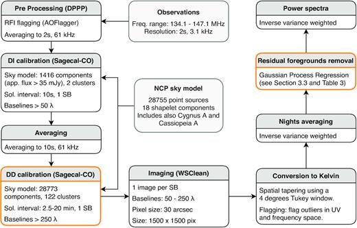
The LOFAR-EoR HBA processing pipeline, describing the steps required to reduce the raw observed visibilities to the 21 cm signal power spectra. The development of the sky-model used at the calibration steps is not described here. The orange outline denotes processes of the pipeline which can have a substantial impact on the 21 cm signal and which are tested through signal injection and simulation (see Section 6.1 and Mevius et al. in preparation).
3.1 Calibration and imaging
In this section, we describe the processes involved in transforming uncalibrated observed visibilities to calibrated, sky-model subtracted image cubes.
3.1.1 RFI flagging
RFI-flagging is done on the highest time and frequency resolution data (2 s, 64 channels per sub-band) using aoflagger11 (Offringa, van de Gronde & Roerdink 2012). The four edge channels of the 64 sub-band channels, each having 3.05 kHz spectral resolution, affected by aliasing from the poly-phase filter, are also flagged. This reduces the effective width of a sub-band to 183 kHz. The data are then averaged to 15 channels (12.2 kHz) per sub-band to reduce the data volume for archiving purposes and further processing (all LOFAR-EoR observations are archived in the LOFAR LTA at surfSARA, and Poznan). It was later found that the data were not correctly flagged during this first RFI flagging stage (the time-window was of insufficient size to correctly detect time-correlated RFI). Since the highest resolution on which the data are archived is 15 channels per sub-band and 2 s, we decided to apply a second RFI flagging on these data before averaging to the three channels and 2 s data product which is used in the initial steps of the calibration. The intrastation baselines of length 127 m share the same electronics cabinet and are prone to correlated RFI generated inside the cabinet itself. Hence, these baselines are also flagged during the pre-processing step. Typically about 5 per cent of visibilities are flagged at this stage (Offringa et al. 2013).
3.1.2 The NCP sky model
The source model components of the NCP field (Bernardi et al. 2010; Yatawatta et al. 2013) has been iteratively built over many years from the highest resolution images, with an angular resolution ≈6 arcsec, using buildsky (Yatawatta et al. 2013). This sky model is composed of 28 773 unpolarized components (28 755 delta functions and 18 shaplets12) covering all sources up to 19 degrees distance from the NCP and down to an apparent flux density of ≈3 mJy inside the primary beam. It also includes Cygnus A about 50° away from the NCP, and Cassiopeia A about 30° away from the NCP, which are the two brightest radio sources in the Northern hemisphere. The spectra of each component are modelled by a third-order polynomial function in log–log space. For modelling some of the brightest sources we have also made use of international baselines in LOFAR, which provide a resolution down to 0.25 arcsec.
The intensity scale of our sky model is set by NVSS J011732+892848 (RA 01h 17m 33s, Dec 89° 28’ 49’ in J2000) (see Fig. 2), a flat spectrum source with an intrinsic flux of 8.1 Jy with 5 per cent accuracy (Patil et al. 2017). The flux and spectrum of this source were obtained following a calibration against 3C 295 in the range 120–160 MHz (Patil et al. 2017). Fig. 2 (top panels) shows images of the NCP field after DI calibration, revealing the sources with flux >3 mJy in the inner 4° × 4° and sources observable at a distance up to 15° from the phase centre (up to the second side-lobe of the LOFAR-HBA primary beam). Many of these sources have complex spatial structure and are modelled by multiple delta functions (or shaplets). The accuracy of our flux scale calibration is tested by cross-identifying the 100 brightest sources observed at a distance <3° from the phase centre with the 6C (Baldwin et al. 1985) and 7C (Hales et al. 2007) 151 MHz radio catalogues. We obtained the intrinsic flux of these sources by first applying a primary-beam correction, and then modelling their spectra over the 13 MHz bandwidth with a power-law to estimate their flux at 151 MHz. We found a mean ratio of 1.02 between our intrinsic flux and the 6C/7C flux with a standard deviation of 0.12, highlighting the accuracy of our absolute flux scale calibration. We additionally found that the night-to-night fluctuations of the flux of these bright sources are on average about 5 per cent, likely due to intrinsic sources fluctuations and primary beam errors not captured by the DI-calibration step.
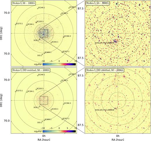
LOFAR-HBA Stokes I continuum images (134–146 MHz) of the NCP field. All 12 nights (≈170 h) were included in making these images. The top panels show the field after DI calibration, with 3C 61.1 subtracted in the visibilities using sagecal, and the images deconvolved using wsclean. The bottom panels show the residual after DD calibration. The left-hand panels show a 34° × 34° image with a resolution of 3.5 arcmin (baselines between 50 and 1000λ) and include the positions of the 3C sources in the field (black circles). The right-hand panels are zoomed 4° × 4° images with a resolution of 42 arcsec (baselines between 50 and 5000λ) in which we also indicate the position of NVSS J011732+892848 (black circle). Power spectra are measured in this 4° × 4° field of view.
3.1.3 Direction-independent calibration
For direction-independent calibration, we use the same approach as described in Patil et al. (2017). Since the relatively bright source in the NCP field, 3C 61.1 (see Fig. 2), is close to the first null of the station’s primary beam, it is necessary to have a separate set of solutions for this direction. In that way we isolate the strong direction-dependent effects of this source. The remainder of the field is modelled by selecting the 1416 brightest components from the NCP sky model, down to an apparent flux limit of 35 mJy. This flux limit was chosen to reduce the processing time while still preserving the signal-to-noise (S/N) required to calibrate the instrument towards these two directions at high time resolution, the power of the remaining sources in the 28 773 components NCP sky model account for only 1 per cent of the total power of the sky model. Calibration is performed on the three channels (61 kHz), and 2 s resolution data set with a spectral and time solution interval of 195.3 kHz (one sub-band) and 10 s, thus allowing us to solve for fast direction-independent ionospheric phase variations. Calibration is done using sagecal-co (Yatawatta 2016), constraining the solutions in frequency with a third-order Bernstein polynomial over 13 MHz bandwidth. sagecal’s consensus optimization distributes the processing over several compute nodes while iteratively penalizing solutions that deviate from a frequency smooth prior by a quadratic regularization term. The frequency smooth prior is updated at each iteration. If given a sufficient number of iterations, this process should converge to this prior. We refer the readers to Yatawatta (2015, 2016) for a more detailed description of the sagecal-co algorithm. In addition to smooth spectral gain variations, we also solve at this stage for the fast frequency varying band-pass response of the stations, which are caused by low-pass and high-pass filters in the signal chain as well as reflections in the coax-cables between tiles and receivers (Offringa et al. 2013; Beardsley et al. 2016; Kern et al. 2020). For this purpose, we use a low regularization parameter and limit the number of iterations to 20. After DI-calibration, outliers in the visibilities (with an amplitude conservatively set to be larger than 70 Jy) are flagged and the data are averaged to the final data product of three channels and 10 s.
3.1.4 Direction-dependent calibration and sky-model subtraction
LOFAR has a wide field-of-view (about 10° between nulls at 140 MHz; van Haarlem et al. 2013) and the visibilities are susceptible to direction-dependent gain variations mainly due to time varying primary beam and ionospheric effects. Therefore, source subtraction is not a simple deconvolution problem and has to be done with the appropriate gain corrections applied along different source directions. Solving for the gains in each direction would be impractical. The extent of the problem is reduced by (i) clustering the sky-model components (Kazemi, Yatawatta & Zaroubi 2013) in a limited number of directions (here we use 122 directions), (ii) constraining the per-sub-band (195.3 kHz) solutions to be spectrally smooth over the 13 MHz bandwidth. The number of clusters, which are typically 1–2 degrees in diameter, is a trade-off between maximizing the S/N inside each cluster and minimizing the cluster size in which all direction-dependent effects (DDE) are assumed to be constant. Constraining the solutions to be spectrally smooth is possible because the earlier direction-independent calibration has taken out most non-smooth instrumental response from the signal chain, and we assume the DDE to be spectrally smooth. We again use sagecal-co (Yatawatta 2016) with a third-order Bernstein polynomial frequency regularization over the 13 MHz bandwidth to solve for the direction-dependent full Stokes gains, represented by a complex 2 × 2 Jones matrix (Hamaker, Bregman & Sault 1996). They incorporate all DDE (at this stage mainly the temporally slow primary beam and ionospheric phase fluctuations). The solution time intervals are chosen between 2.5 and 20 min, depending on the apparent total flux in each cluster. This should be adequate for capturing primary beam changes over time, but not for the fast ionospheric phase variations on most baselines (Vedantham & Koopmans 2016). In the future, we plan to investigate the reduction of this solution time interval and to decouple the phase and amplitude solution time (e.g. van Weeren et al. 2016).
sagecal-co uses a consensus optimization with an alternating direction method of multipliers (ADMM) algorithm to efficiently solve for all clusters and all sub-bands simultaneously. The gain solution is constrained to approach a smooth curve by a regularization prior. As for DI-calibration, here we again use the Bernstein polynomial basis function. We use a total of 40 ADMM iterations, which we found to be sufficient to achieve the required convergence. The regularization parameter must be carefully chosen for the fitting process to converge while still enforcing sufficient smoothness. Low or no regularization will effectively overfit the data, resulting in signal suppression at the smallest baselines where we are most sensitive to the 21 cm signal (Patil et al. 2016). The solution adopted in Patil et al. (2017) is to split the baseline set into non-overlapping calibration and 21 cm signal analysis subsets. We chose to exclude the baselines |$\lt \!250\, \lambda$| in DD calibration. This limit is chosen as a compromise: (i) the lower set includes the baselines lengths where we are most sensitive to the 21 cm signal, (ii) it excludes from the calibration the baselines at which the Galactic diffuse emission, not included in our sky-model, starts to be significant, (iii) it still includes enough baselines in the calibration to reach the required S/N. The downside is that the calibration errors now cause excess noise for the baselines not part of the calibration (an effect that was investigated in detail in Patil et al. 2016). This additional source of noise can be mitigated by adequately enforcing spectrally smooth solutions, which has the combined benefit of reducing calibration errors, improving the convergence rate, and smoothing the remaining calibration errors along the frequency direction (Yatawatta 2015; Barry et al. 2016). Mouri Sardarabadi & Koopmans (2019) have theoretically quantified the level of the expected signal suppression and leakage from direction-dependent calibration. By excluding the |$\lt \!250\, \lambda$| baselines during calibration and enforcing spectral smoothness of the gains, they found no signal loss on the baselines of interest and limited amplification for |$k_{\parallel }$| modes below |$0.15\, \mathrm{h\, cMpc^{-1}}$|. Even when considering sky-model incompleteness and that spectral smoothness is only partially achieved, very limited suppression of maximally 5 per cent is observed. We confirm these results experimentally (Mevius et al. in preparation) using signals injected in to the data and a setup identical to our observational and processing setup.
The regularization parameters and number of iterations adopted in Patil et al. (2017) were later found to be sub-optimal: the convergence was never reached, resulting in relatively high excess noise. For the analysis presented here, significant focus is placed on improving this aspect. We tested increasing regularization values over a limited set of visibilities (about 1 h of data) by evaluating the ADMM residuals after each iteration to assess the convergence and gain in signal-to-noise ratio. The latter is calculated for every gain-direction (hence cluster of sky-model components) individually and is defined as the ratio of the mean of the gain solution over the standard deviation of the sub-band gain differences. For each individual cluster, we select the regularization value that maximizes the above-mentioned ratio (Mevius et al. in preparation). Compared to Patil et al. (2017) this ratio is improved by a factor of five. For most clusters, we now reach an S/N ratio ≳20, with clusters inside the first lobe of the primary lobe closer to an S/N ratio of 100 or above (Mevius et al., in preparation).
Gain-corrected sky-model visibilities are computed after DD-calibration by applying the gain solutions to the predicted sky-model visibilities for each cluster, and subsequently subtracting these from the observed visibilities. Fig. 2 (bottom panels) shows residual images of the NCP field after DD calibration. While most of the sources have been correctly subtracted, the brightest sources leave residuals with flux between −50 and +50 mJy.
3.1.5 Imaging after sky-model subtraction
Residual visibilities obtained after calibration and source subtraction are gridded and imaged independently for each sub-band using wsclean13 (Offringa et al. 2014), creating an (l, m, ν) image cube. Recently, several studies analysed the impact of visibility gridding on the 21 cm signal power spectra. Offringa et al. (2019a) assessed the impact of missing data due to RFI flagging and found that the combination of flagging and averaging causes tiny spectral fluctuations, resulting in ‘flagging excess power’ which can be mitigated to a sufficient level by sky-model subtraction before gridding and by using unitary weighted visibilities during gridding.14 The impact of the gridding algorithm itself is also assessed in Offringa et al. (2019b), and a minimum requirement on various gridding parameters is prescribed. In this work we follow all these recommendations: (i) our sky-model is subtracted by sagecal before gridding, (ii) we use unit weighting during gridding, (iii) we use a Kaiser-Bessel anti-aliasing filter with a kernel size of 15 pixels and an oversampling factor of 4095, along with 32 w layers. These ensure that any systematics due to gridding are confined significantly below the predicted 21 cm signal and thermal noise (see fig. 8 in Offringa et al. 2019a and fig. 5 in Offringa et al. 2019b).
Stokes I and V images in Jy PSF−1 and point-spread function (PSF) maps are produced with natural weighting for each sub-band separately. We also create even and odd 10 s time-step images to generate gridded time-difference visibilities, which are used to estimate the thermal noise variance in the data. We then combine the different sub-bands to form image cubes with a field of view of 12° × 12° and 0.5 arcmin pixel size and these are subsequently trimmed using a Tukey (i.e. tapered cosine) spatial filter with a diameter of 4°. This ensures that we reduce our analysis to the most sensitive part of the primary beam, which has a full width at half-maximum (FWHM) at 140 MHz of ≈4.1°, and avoid the uncertainties of the primary beam at a substantial distance from the beam centre. We choose a Tukey window as a compromise between avoiding sharp edges when trimming the images and maximizing the observed volume (i.e. maximizing the sensitivity).
3.2 Conversion to brightness temperature and the combination of power spectra
Here we discuss how visibilities are converted to brightness temperature and how data are averaged both per night of observations and between nights.
3.2.1 Conversion to brightness temperature
For each analysed data set, we store the gridded visibilities V(u, v, ν) in HDF5 format in units of Kelvin, along with the numbers of visibilities that went into each (u, v, ν) grid point, Nvis(u, v, ν).
3.2.2 Outlier flagging
We use a k-sigma clipping method with detrending, to flag outliers in the gridded visibility cubes. These are likely due to low-level RFI not flagged by aoflagger or due to non-converged gain solutions. Sub-band outliers are flagged based on their Stokes-V and Stokes-I variance, while (u, v) grid outliers are flagged based on their Stokes-V and sub-band-difference Stokes-I variance. Depending on the data set, we found that about 20–35 per cent of the sub-bands and about 5–10 per cent of uv-cells are flagged. At this stage, we are very conservative in our approach to flagging data, favouring less data rather than bad data. These ratios could be reduced in the future by improving low-level RFI flagging before visibilities gridding, and using new algorithms able to filter certain type of RFI instead of flagging them.
3.2.3 Noise statistics and weight estimates
Another noise estimate can be derived from the visibility difference between sub-bands, δνV(u, v, ν), which should better reflect the spectrally uncorrelated noise in the data. Compared to the time difference noise spectrum (in baseline-frequency space), we find that the sub-band difference noise variance is on average higher by a factor ≈1.35 for Stokes V and ≈2 for Stokes I (sixth and seventh columns of Table 1, respectively) with a small night-to-night variation. We also find that this additional spectrally uncorrelated noise term is dependent on the baseline length, with the ratio of the sub-band difference over time difference noise spectrum gradually increasing as a function of decreasing baseline length. A similar trend is observed for both Stokes I and V (see Fig. 3).
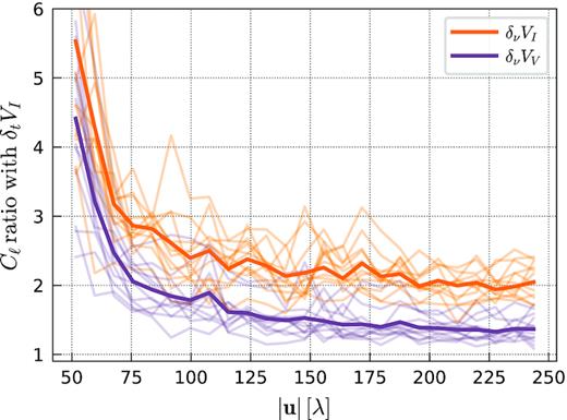
Ratio between sub-band difference and time difference angular power spectra for Stokes I (orange lines) and Stokes V (magenta lines). All nights are shown, and the average over all nights is indicated by thicker line.
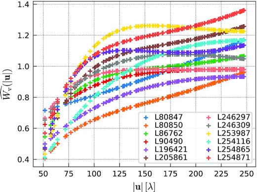
Weights scaling factor |$\widehat{W_\mathrm{v}}$| as a function of baseline length, for all nights (one colour per night).
3.2.4 Averaging multiple nights
3.3 Residual foreground removal
After direction-dependent calibration and subtraction of the gain-corrected sky model, the residual Stokes I visibilities are composed of extragalactic emission below the confusion limit (and thus not removable by source subtraction) and partially polarized diffuse Galactic emission which is still approximately three orders of magnitude brighter than the 21 cm signal. The emission mechanism of these foreground sources (predominantly synchrotron and free–free emission) are well-known to vary smoothly in frequency, and this characteristic can differentiate them from the rapidly fluctuating 21 cm signal (Shaver et al. 1999; Jelić et al. 2008). However, the interaction of the spectrally smooth foregrounds with the Earth’s ionosphere, the inherent chromatic nature of our observing instrument (in both the PSF and the primary beam), and chromatic calibration errors create additional ‘mode-mixing’ foreground contaminants which introduce spectral structure to the otherwise smooth foregrounds (Datta et al. 2010; Morales et al. 2012; Trott et al. 2012; Vedantham et al. 2012).
In the 2D angular (k⊥) versus line-of-sight (|$k_{\parallel }$|) power spectra, the foregrounds and mode-mixing contaminants are primarily localized inside a wedge-like region.15 This makes them separable from the 21 cm signal by either avoiding the predominantly foreground-contaminated region and only probe a k-space region where the 21 cm signal dominates (foreground avoidance strategy; e.g. Liu et al. 2014a; Trott et al. 2016), or by exploiting their different spectral (and spatial) correlation signature to separate them (foreground removal strategy; e.g. Chapman et al. 2012, 2013; Patil et al. 2017; Mertens et al. 2018).
We adopt a foreground removal strategy which, if done correctly, has the advantage of considerably increasing our sensitivity to larger comoving scales (smaller k-modes) (Pober et al. 2014). To that aim, we developed a novel foregrounds removal technique based on GPR (Mertens et al. 2018). In this framework, the different components of the observations, including the astrophysical foregrounds, mode-mixing contaminants, and the 21 cm signal, are modelled as a Gaussian Process (GP). A GP is the joint distribution of a collection of normally distributed random variables (Rasmussen & Williams 2005). The sum of the covariances of these distributions, which define the covariance between pairs of observations (e.g. at different frequencies), is specified by parametrizable covariance functions. The covariance function determines the structure that the GP will be able to model. In GPR, we use the GP as parametrized priors, and the Bayesian likelihood of the model is estimated by conditioning this prior to the observations. Standard optimization or Monte Carlo Markov Chain (MCMC) methods can be used to determine the optimal hyperparameters of the covariance functions. The GPR method is closely related to Wiener filtering (Zaroubi et al. 1995; Särkkä & Solin 2013). Compared to the Generalized Morphological Component Analysis (GMCA; Bobin et al. 2008; Chapman et al. 2013) used in Patil et al. (2017), GPR is more suited to treat the problem of foregrounds in high redshift 21 cm experiments (Mertens et al. 2018) and reduces the risk of signal suppression by explicitly incorporating a 21 cm signal covariance prior in its GP covariance model.
3.3.1 Gaussian process regression
We use an exponential covariance function for the 21 cm signal, as we found that it was able to match well the frequency covariance from a simulated 21 cm signal (Mertens et al. 2018). Eventually, the choice of the covariance functions is data driven, in a Bayesian sense, selecting the one that maximizes the evidence. We will see in Section 4 that the simple foregrounds +21 cm dichotomy will need to be adapted, introducing an additional component, to match the data better.
3.3.2 Bias corrections
3.4 Power spectra estimation
The uncertainties on the power spectra reported here are sample variance taking into account the number of individual uv-cells averaged, and the effective observed field-of-view given by the primary beam Apb(l, m) and spatial tapering function Aw(l, m). They assume that all averaged uv-cells are independent measurements.17 All residual and noise power spectra are computed without a frequency-tapering function to benefit from the full bandwidth sensitivity. In the case of GPR residuals, we have another source of uncertainty which comes from the uncertainty on the GP model hyperparameters. These can be propagated using an MCMC method (see Appendix B). This calculation shows it to be negligible compared to the sample variance and it can be ignored in our calculations (see also Mertens et al. 2018).
4 RESULTS FROM NIGHT TO NIGHT
In this section we discuss the results of processing the data from each night individually. We start by assessing the improvement made to the data processing compared to Patil et al. (2017). The residual foregrounds (after DD calibration) and noise in the data are analysed and we examine the residual image cubes after GPR foreground removal, and its night-to-night correlation.
4.1 Power spectra before foreground removal
All nights are calibrated and imaged following the procedure described in Section 3.
4.1.1 Calibration improvements
To demonstrate the improvement in the calibration, we process one night of observation (L246309) with the DD calibration regularization parameters used in Patil et al. (2017). Mevius et al. (in preparation) show that the latter approach leads to substantial excess noise (beyond thermal noise), in particular if the constraints on spectral smoothness are not correctly enforced. This leads to excess noise on baselines |$\lt\! 250\, \lambda$| because of overfitting (see also Mouri Sardarabadi & Koopmans 2019). Cylindrically averaged power spectra of Stokes I and Stokes V for the two calibration procedures (old versus new) are shown in Figs 5 and 6, indicating a significant decrease of the excess noise, while leaving the residual foregrounds largely unaffected. Taking the difference between the old and new procedures shows that the excess noise is reduced in both Stokes I and Stokes V in a similar manner (see Fig. 6). This excess noise is mostly spectrally uncorrelated and close to constant as a function of |$k_{\parallel }$|, with the small increase of power at |$k_{\parallel } \lt 0.2 \mathrm{h\, cMpc^{-1}}$| related to the basis function adopted as frequency gain constraint. This is in good agreement with the theoretical predictions from Mouri Sardarabadi & Koopmans (2019). With the new procedure, the Stokes V power is now also closer to the thermal noise power.
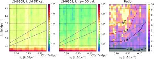
Improvement due to the new calibration for a single night of observation. We compare the new DD calibration procedure (middle panel) against the one adopted in Patil et al. (2017) (left-hand panel). The ratio of the two (right-hand panel) shows a substantial reduction of the excess noise related to the 250λ baseline cut overfitting effect (by a factor >5 for |$k_{\parallel } \gt 0.8 \mathrm{h\, cMpc^{-1}}$|), with no impact on the residual foregrounds (ratio ∼1 at low |$k_{\parallel }$|). The plain grey lines indicate, from bottom to top, 50° and instrumental horizon delay lines (delimiting the foreground wedge).
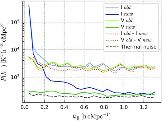
Improvement due to the new calibration for a single night of observation. Here we compare Stokes I (blue lines) and Stokes V (green lines) cylindrically averaged power spectra (averaged over all baselines) processed with the new DD calibration procedure (new) against the one used in Patil et al. (2017) (old). The excess noise (difference between old and new) is reduced similarly in Stokes I (orange line) and Stokes V (red line). The thermal noise power is indicated by the dashed grey line.
4.1.2 Residual foregrounds
Fig. 7 shows the total intensity variance and angular power spectra at different steps of processing. The foreground power is reduced by a factor of ∼500 after DD calibration. The residual power is consistent between nights, with a night-to-night relative variation of |$\approx 12 {{\ \rm per\ cent}}$|. The Stokes I angular power spectra are relatively flat before sky-model subtraction, while afterwards, the power towards the larger scales (smaller baselines) increases, consistent with a power law with a spatial slope βℓ ≈ −1.18. On large scales, the observed residual power, |$C_{\ell } (|\mathbf {u}| = 50 \lambda) \sim 10^3\, \mathrm{mK^2}$|, is comparable with the power attributed to the Galactic foregrounds in the NCP field observation from Bernardi et al. (2010) using the Westerbork telescope. However, the spatial slope does not match the expectation from Galactic diffuse emission, in the range [−2, −3] (Bernardi et al. 2010). This suggests that the residual power observed here is a combination of Galactic emission, residual confusion-limited extragalactic sources, and calibration errors from the DD-calibration stage. The latter may be substantial (see e.g Mouri Sardarabadi & Koopmans 2019), but because they are now mostly frequency coherent (resulting from the high regularization used in the consensus optimization), they are separable from the 21 cm signal and can be removed using the GPR method.
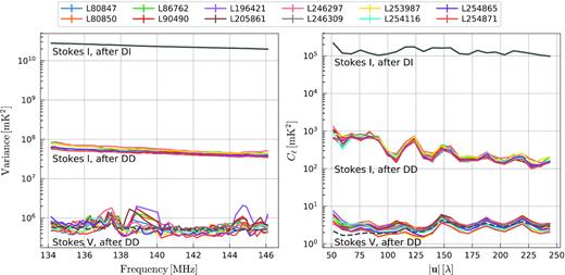
Variance (left-hand panel) and angular power spectra (right-hand panel) for all nights at different processing stages. Different nights are indicated by a different colour. The top lines show the Stokes I power after DI calibration. The middle lines show the Stokes I power after DD calibration and sky model subtraction (but before GPR). The lines at the bottom show the Stokes V sub-band difference power. The black dashed line represent the thermal noise power for an average observing duration time (14.4 h) and an average SEFD (4150 Jy).
4.1.3 Noise statistics
Following the procedure detailed in Section 3.2.3, Stokes V and Stokes I sub-band difference power spectra (δνI and δνV, respectively) are generated as a proxy for spectrally uncorrelated noise, and time-difference power spectra from even/odd sets are generated as a proxy for the thermal noise power spectra (δtV). Taking the power ratio of δνV over δtV, exhibits a non-negligible excess power well above the thermal noise level (|$\approx \! 35{{\ \rm per\ cent}}$|, see Table 1). This additional spectrally uncorrelated noise is baseline dependent, with a flat ratio of |$\approx \! 1.25$| for baselines of length |$\gt 125\, \lambda$|, and then gradually increasing to smaller baselines (see Figs 7 and 3). The ratio also varies considerably from night to night. Examining the power ratio of δνV over δνI, shows a higher sub-band difference noise level (by a factor |$\approx \!50{{\ \rm per\ cent}}$|) in Stokes I. This ratio has a weak dependence on the baseline length (with a Pearson correlation coefficient between ratio and baselines r = 0.23 and a corresponding p-value <10−5).
This source of noise is still being investigated. One hypothesis is mutual-coupling between spatially close stations (e.g. Fagnoni et al. 2019). This would explain the rise of power with decreasing baseline length. It might also be a source of broad-band and faint RFI at the central LOFAR ‘superterp’ region. It is also interesting to note that the Galactic diffuse emission is prominent at baselines |$\lt\! 125\, \lambda$|. Each of these effects will be further analysed in future publications.
4.2 Residual foreground removal
The residual foreground emission after DD calibration is removed using GPR modelling which is applied to the same gridded visibilities (4° × 4° field of view) as used for the power spectrum analysis.
4.2.1 Covariance model
In Section 3.3 it was shown that we can recover unbiased power spectra of the signal as long as the covariance model matches the data. The GP model therefore needs to be as comprehensive as possible, incorporating covariance functions for all components of the data, including the 21 cm signal and known systematics. The selection of the covariance functions is driven by the data in a Bayesian framework, by selecting the model that maximizes the evidence. Because these covariance functions are parametrized, they too are optimized.
- (1) The foregrounds – At this stage, the foreground residuals are mainly composed of intrinsic sky emission from confusion-limited extragalactic sources and from our own Galaxy, and of mode-mixing contaminants related to e.g. the instrument chromaticity and calibration errors that can originate from all sources in the sky leaking into the 4° × 4° image cubes through their side lobes. We build this property into the GP spectral-covariance model by decomposing the foreground covariance matrix into two separate parts,with ‘sky’ denoting the intrinsic sky and ‘mix’ denoting the mode-mixing contaminants. A Matern covariance function is adopted for each of the components of the GP model of the data, which is defined as (Stein 1999):(28)$$\begin{eqnarray*} K_{\mathrm{fg}} = K_{\mathrm{sky}} + K_{\mathrm{mix}}, \end{eqnarray*}$$where σ2 is the variance, r = |νq − νp| is the absolute difference between the frequencies of two sub-bands, and Kη is the modified Bessel function of the second kind. The parameter η controls the smoothness of the resulting function. Functions obtained with this class of kernels are at least η-times differentiable. The kernel is also parametrized by the hyperparameter l, which is the characteristic scale over which the spectrum is coherent. Setting η to ∞ yields a Gaussian covariance function, also known as the radial basis function, which is well-adapted to model the intrinsic (sky) foreground emission (Mertens et al. 2018). The coherence scale of this component is usually large, and we adopt a uniform prior |$\mathcal {U}(10, 100)$| MHz for lsky. For the mode-mixing component, several covariance functions are evaluated. We test the Matern covariance function with different values of ηmix (|$+\inf$|, 5/2 and 3/2), and also the Rational Quadratic function (κRatQuad) which was used recently in Gehlot et al. (2019) to model the foreground contaminants of LOFAR-LBA data. A Matern kernel with ηmix = 3/2 is favoured by the data when comparing the Bayes factor (the ratio of the evidence of one hypothesis to the evidence of another), with very strong evidence against a wide range of alternatives (see Table 2 for a comparison of all tested GP models). A uniform prior |$l_{\mathrm{mix}} \sim \mathcal {U}(1,10)$| is adopted, because simulations show that the foreground signal is separable from the 21 cm signal as long as lmix ≳ 1 MHz (Mertens et al. 2018).(29)$$\begin{eqnarray*} \kappa _{\mathrm{Matern}}(\nu _p, \nu _q) = \sigma ^2 \frac{2^{1 - \eta }}{\Gamma (\eta)}\left(\frac{\sqrt{2\eta }r}{l}\right)^{\eta }K_{\eta }\left(\frac{\sqrt{2\eta }r}{l}\right), \end{eqnarray*}$$
(2) The 21 cm signal – The covariance shape of the real 21 cm signal is not known. However, information from current 21 cm simulations can be used to assess which family of models is a good approximation of the 21 cm signal. Mertens et al. (2018) show that the 21 cm signal frequency covariance – calculated using 21cmFAST (Mesinger et al. 2011) – can be well-approximated by an exponential covariance function (i.e. a Matern function with η = 1/2). This function has two hyperparameters: the frequency coherence scale l21 and a variance |$\sigma ^2_{21}$|. These allow some degree of freedom to match different phases of reionization. Based on the covariance of 21 cmFAST simulations at different redshifts (see fig. 2 in Mertens et al. 2018), a uniform prior |$\mathcal {U}(0.1,1.2)$| MHz on l21 is adopted.
(3) The noise – Various noise estimators can be used to build the noise covariance. The time-differenced visibilities – obtained from the difference between even and odd sets of visibilities (e.g. separated by only several seconds) – is expected to be an excellent estimator of the thermal noise. It does, however, not fully reflect the spectrally uncorrelated random errors in our data (e.g. due to increased noise at short baselines; see Section 4.1.3). An alternative is to use Stokes V, which has previously been used as a noise estimator (Patil et al. 2017). It, however, can be corrupted by polarization leakage from Stokes I. The difference between alternating sub-bands in Stokes V can also be a good noise estimator, but it introduces correlation between consecutive sub-bands. The solution that is adopted is to simulate the noise covariance |$K_{\mathrm{v_sn}}$| that we will use in our GP model using the weights in equation (6) and the noise definition of the gridded visibilities in equation (4). This estimator is based on Stokes V noise, while the actual noise in Stokes I can be slightly higher (see Section 3.2.3 and Table 1). A noise scaling factor αn is therefore adopted, which is optimized along with the other hyperparameters of the GP model, resulting in the final noise covariance |$\rm K^{\prime }_{\mathrm{sn}} = \alpha _n K_{\mathrm{sn}}$|. An associated noise data set VN(u, v, ν) is built to compute the noise power spectra and is used to subtract the noise bias from the residual power spectra.
(4) The excess noise – After applying GPR using foreground, 21 cm signal and noise-only covariance models, a significant spectrally correlated residual is still present. This ‘excess noise or power’ is accommodated in the model by an additional Matern covariance kernel Kex. Different values of ηex were tested and ηex = 5/2 is strongly favoured by the data. Adding this ‘excess’ component to the model significantly increases the Bayesian evidence (see Table 2), motivating this choice.
Different GP models assessed against the fiducial GP model, being a Matern kernel with ηmix = 3/2 (see Section 4.2.1). Negative values of the difference in log-evidence (|$\cal Z$|) indicate a less probable model. A difference of |$|\Delta {\cal Z}|\gt 20$| is typically regarded as a very strong difference in evidence.
| Model change | |$\Delta {\cal Z}$| |
|---|---|
| ηex = 5/2, ηmix = 3/2 (fiducial) | 0 |
| ηmix = 5/2 | −39 |
| ηmix = +∞ | −147 |
| κmix ≡ κRatQuad | −7 |
| αn = 1 (fixed) | −110 |
| |$\sigma ^2_{\mathrm{ex}} = 0$| (fixed) | −149 |
| ηex = 3/2 | −17 |
| Model change | |$\Delta {\cal Z}$| |
|---|---|
| ηex = 5/2, ηmix = 3/2 (fiducial) | 0 |
| ηmix = 5/2 | −39 |
| ηmix = +∞ | −147 |
| κmix ≡ κRatQuad | −7 |
| αn = 1 (fixed) | −110 |
| |$\sigma ^2_{\mathrm{ex}} = 0$| (fixed) | −149 |
| ηex = 3/2 | −17 |
Summary of the GP model, the priors on its hyperparameters, and the estimated median and 68 per cent confidence intervals obtained using an MCMC procedure for the 10 nights data set (see Appendix B. All covariance functions are Matern functions.
| Hyperparameter | Prior | MCMC estimate (10 nights) |
|---|---|---|
| ηsky | +∞ | − |
| |$\sigma ^2_{\mathrm{sky}} / \sigma ^2_{\mathrm{n}}$| | − | |$611\substack{+22\\-19}$| |
| lsky | |$\mathcal {U}(10, 100)$| | |$47.5\substack{+3.1\\-2.8}$| |
| ηmix | 3/2 | − |
| |$\sigma ^2_{\mathrm{mix}} / \sigma ^2_{\mathrm{n}}$| | − | |$50.4\substack{+2.1\\-1.9}$| |
| lmix | |$\mathcal {U}(1, 10)$| | |$2.97\substack{+0.09\\-0.08}$| |
| ηex | 5/2 | − |
| |$\sigma ^2_{\mathrm{ex}} / \sigma ^2_{\mathrm{n}}$| | − | |$2.18\substack{+0.09\\-0.14}$| |
| lex | |$\mathcal {U}(0.2, 0.8)$| | |$0.26\substack{+0.01\\-0.01}$| |
| η21 | 1/2 | − |
| |$\sigma ^2_{\mathrm{21}} / \sigma ^2_{\mathrm{n}}$| | − | <0.77 |
| l21 | |$\mathcal {U}(0.1, 1.2)$| | >0.73a |
| αn | − | |$1.17\substack{+0.06\\-0.06}$| |
Note. aThe upper confidence interval hits the prior boundaries, hence we report here only the lower limit.
4.2.2 Power spectra after foreground removal
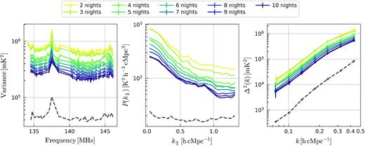
Fig. 8 shows the variance and power spectra of the residual after GPR foreground removal for all nights, compared to the expected thermal noise level for an average observing duration time of 14.4 h with an SEFD of 4150 Jy. For all nights, the excess power per sub-band is a factor of 2–3 times higher than the thermal noise. This excess corresponds to the ‘excess’ component of our GP model which is not removed from the data due to its small frequency coherence scale. At small |$k_{\parallel }$|, the ratio of residual to thermal noise power is ≈5–10, while it is ≈1–2 at large |$k_{\parallel }$|. The same can be seen in the spherically averaged power spectra. Night-to-night variations of the residual power is a factor 2–3 and cannot be explained by the different total observing times between nights. For example, the excess power in LOFAR observing-cycle 2 observations is below that for cycles 0 and 1. Different ionospheric or RFI conditions might contribute to these night-to-night variations. Hence, although this excess power is drastically lower than in Patil et al. (2017) due to improved calibration, it is still not entirely mitigated. Below we investigate the excess power in more detail.
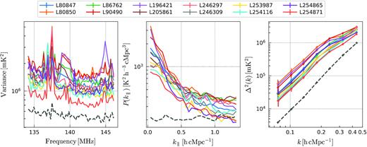
Variance (left-hand panel), cylindrically averaged power spectra (averaged over all baselines) (middle panel) and spherically averaged power spectra (right-hand panel) of Stokes I after GPR residual foreground removal, for all nights analysed in this work. The black dashed line represent the thermal noise power for an average observing duration time (14.4 h) and an average SEFD (4150 Jy). At high |$k_{\parallel }$|, the residual power after GPR is close to the thermal noise level, but a frequency correlated excess power is present. Note that the noise bias has not been removed here.
4.3 Night-to-night correlations between residuals
A corner-plot of the correlations between nights is presented in Fig. 9 for each of the three different regions. We also show the correlation coefficients as a function of their difference in the start of the observations in Local Siderial Time (LST) versus their start in number of (Julian) days. This representation provides additional clues about the different observing conditions between nights. In the ‘EoR window’, only very small correlations are observed. The correlation is on average slightly larger for the shorter baselines (≈0.04, significance >0.032) than for the larger baselines (≈0.02, significance >0.018), as defined above. Significantly larger correlations are found in the ‘foregrounds wedge’ region (≈0.03–0.25, significance >0.018). For each of the three regions, also a clear trend between the correlation coefficients and either difference in Julian date (between nights) or LST are found: correlations are larger if the observations are either close in Julian date or close in LST, and largest if they are close in both, hence they observe the same sky during the observing runs with a similar primary beam and a similar PSF. The largest correlation, in particular inside the wedge region, is found when two nights are close and separated by only a small number of days. This suggests that some of the excess power in the data residuals (after sky-model and foreground subtraction) originates from sky emission that is far from the phase centre for which the primary beam will change considerably at different values of the LST. The PSF will also change but, for all nights, the uv-plane is always fully sampled in the 50–250λ range, given the long (12–16h) duration of our observing nights. For the shorter baselines and in the ‘EoR window’ region, the trend with LST difference is less pronounced, which suggests that part of the additional noise at baselines <100λ discussed in Section 4.1.3 may have a local origin (e.g. RFI). These are all baselines from stations in the superterp and might arise from mutual-coupling. Its origin will be investigated in the future using a near-field imaging technique (Paciga et al. 2011).
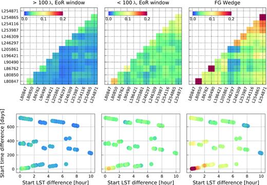
Top: Cross-coherence matrix between all nights after GPR foregrounds removal. Three different regions of the cylindrically averaged power spectra are analysed: The EoR window for baselines |$\gt \!100\, \lambda$| (left-hand panel), the EoR window for baselines |$\lt\! 100\, \lambda$| (middle panel), and the foreground wedge region for baselines |$\gt \!100\, \lambda$| (right-hand panel). We note there is no or a small correlation in the EoR window, while the correlation is more noticeable in the foreground wedge, especially for certain combinations of nights. Bottom: Cross-coherence (colour scale) between two nights as a function of LST time difference (abscissa) and UTC time difference (ordinate). We observe higher correlation between observation started at the same LST time (which will see the same sky throughout the observation).
Based on this analysis, we discard nights L80850 and L254871 as the former has a high residual power and both have a high correlation coefficient between their residuals with other nights. This leaves a total of ten nights for further analysis.
5 COMBINING DATA SETS
In this section, we discuss the power spectra obtained by combining the ten selected nights of observations, corresponding to about 141 h of data.
5.1 Weighted averaging of the data
The gridded visibilities of separate nightly data sets are averaged following the procedure described in Section 3.2.4. They are combined in the order of their date of observation.19 Intermediate data sets are also kept, yielding a total of nine combined data sets with an increasing total observation time. For each accumulated data set, the residual foregrounds are estimated and subtracted following the same GPR procedure and GP covariance model described in Section 4.2. Hence, the GPR is only applied to the combined data sets.
When combining the data, the GP spectral coherence scales of the foregrounds converge to similar values as found from individual nights. This suggests that these scales are stable between nights. The GP variances for the ‘sky’ and ‘mix’ components also do not vary much when compared to the total variance (≈0.85–0.9 for the ‘sky’ component, and ≈0.04–0.065 for the ‘mix’ component). This is expected for a signal that is coherent over nights. The GP variance of the ‘excess’ component decreases with increasing total observation time. It does not decrease, however, as would be expected from uncorrelated noise, with a ratio |$\approx \! 2.2$| found between the two nights data set (28 h) and ten nights data set (141 h), confirming that the ‘excess’ component partly correlates between nights. The most probable hyperparameter values for the combined (i.e. ten nights) data set are given in Table 3, with their confidence intervals obtained using an MCMC procedure (see Appendix B and Mertens et al. 2018). Most parameters are well constrained, except the variance of the ‘21 cm signal’ component which is consistent with zero, as expected for such a short total integration time, and the coherence-scale of the ‘21 cm signal’ for which the upper bound of the posterior distribution hit the prior boundary, also the significance of the later is reduced given the non-significant variance of this component. Hence only upper limits on the 21 cm signal (power spectra) can be given.
5.2 Residual power spectra
Fig. 10 shows the power spectrum and its integrated variance after applying GPR, but before subtracting the noise bias, as we combine more data. The frequency range of 136–140 MHz is heavily affected by RFI and many of the corresponding sub-bands are therefore discarded. The results are compared to the thermal noise power estimated from the 10 s time difference visibilities. The data are combined (i.e. integrated) in the order of the observation. The integrated variance as a function of frequency (left-hand panel) shows a gradual reduction of power as we combine more data. However, taking the ratio between the 2 and 10 nights of accumulated data, a value of ≈3 is found while theoretically a ratio closer to ≈5 is expected. Examining the power spectra as a function of |$k_{\parallel }$| (middle panel) shows that the ratio of residual power over thermal noise is worse in the foreground-dominated region (i.e. inside the ‘wedge’), where only a reduction in power of ≈2.8 is found. At |$k_{\parallel } \gt 1 \mathrm{h\, cMpc^{-1}}$|, the ratio is closer to ≈4. Comparing the residual power to the thermal-noise power in the spherically averaged power spectrum (right-hand panel), the residual power is found to be ≈14 times the thermal noise power at |$k \approx 0.08 \mathrm{h\, cMpc^{-1}}$|, and about ≈6 times the thermal noise power at |$k \approx 0.45\mathrm{h\, cMpc^{-1}}$|.
Variance (left-hand panel), cylindrically averaged power spectra (averaged over all baselines) (middle panel), and spherically averaged power spectra (right-hand panel) of Stokes I after GPR residual foreground removal, as we combine the nights, from 2 (yellow) to 10 (dark blue). The black dashed line represent the thermal noise power of the 10 nights data set, estimated from 10 s time difference visibilities. Note that the noise bias is not removed here.
In Fig. 11, we compare the cylindrically averaged power spectra of the 10 nights data set residual (middle panel) to a 1 night equivalent data set power spectrum in which the different nights are averaged incoherently (i.e. averaged in power spectra) (left-hand panel). Taking the ratio of the two (right-hand panel), we observe a ratio ≈4 in the foreground wedge region and ≈5–6 outside it where a ratio of 10 is expected. This indicates that the night-to-night correlation of the residual is not just limited to the wedge, where some residual sky foregrounds might be expected, but also affects the EoR window. Even at high |$k_{\parallel }$|, the residuals are not thermal noise dominated in the combined data set. This night-to-night correlation of the residuals, that we also observed in Section 4.3, is the major challenge that needs to be understood and solved in the future as it limits our ability to integrate >200 h of data. Possible origins will be discussed in Section 6.

Cylindrical Stokes I power spectra after GPR residual foreground removal of the 10 nights incoherently averaged (left-hand panel) and coherently averaged (middle panel). Both are optimally combined and thus the ratio of the two (right-hand panel) is expected to be 10 in the case of uncorrelated residuals. We observe significant residuals in the foreground wedge region, especially below the 50° delay line (black lines), for both the incoherently and coherently averaged cases. The ratio of the two is <5 in this region, suggesting frequency correlated excess power which is also partially correlated between nights.
5.2.1 Residual over thermal-noise power ratio
Fig. 12 shows the ratio of the power spectrum of the Stokes I residuals over the observed noise power spectrum (left-hand panel) and over the thermal noise power spectrum (right-hand panel). The noise power spectrum is computed from the simulated noise data set VN(u, v, ν) used in the GP model (see Section 4.2.1) and accounts for the larger spectrally uncorrelated noise level observed on baseline lengths of |$\lt\! 125\, \lambda$| as compared to the thermal noise. Hence, it incorporates the noise scaling factor αn which is optimized as part of the GP covariance model. The residual of the Stokes I over the observed noise ratio shows that the GP model properly accounts for the spectrally uncorrelated noise in the data: a ratio ∼1 is reached at |$k_{\parallel } \gt 1 \mathrm{h\, cMpc^{-1}}$|. At lower values of |$k_{\parallel }$|, however, the ratio gradually increases. This is the spectrally correlated excess power, which is also part of the GP model, but is not part of the foreground covariance model. Remarkably, the ratio appears to be baseline independent, indicating that the excess power follows the same baseline dependence as the noise (which corresponds to the uv-density). Examining the ratio of the residual over the thermal noise shows that it increases towards shorter baseline lengths.
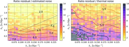
Ratio of cylindrical Stokes I power spectra of the 10 nights Stokes I after GPR residual foreground removal over the noise estimated by GPR (left-hand panel) and the thermal noise estimated from 10 s time difference visibilities (right-hand panel). The excess power (against the frequency uncorrelated noise) does not show strong baselines dependence. The baseline dependence of the excess noise (described in Section 4.1.3) is striking when compared against the thermal noise.
In summary, the residual power spectrum from the combined data set, after GPR foreground removal, can be decomposed into (i) thermal noise, (ii) an additional noise-like component that is spectrally uncorrelated, and (iii) an excess noise that is partially correlated between nights and spectrally correlated (i.e. its power spectrum in delay space is not white) and cannot be removed by the GPR method as part of the spectrally smooth foregrounds. The noise power is still significantly larger than the thermal noise power, especially on shorter baseline lengths, although the excess is much smaller than found in Patil et al. (2017) due to the signal-processing improvements presented in this paper.
5.3 Upper limit on the 21 cm signal power spectrum
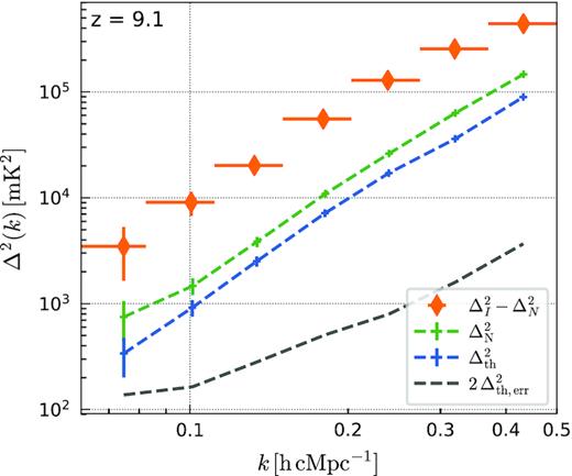
Final 10 nights Stokes I spherically averaged power spectra after GPR residual foreground removal and noise bias removal (orange). The green and blue dashed lines represent, respectively, the estimated frequency uncorrelated noise and thermal noise power of the 10 nights data set. The black dashed line represents the 2 − σ upper limit theoretically achievable if the residual of the 10 nights data set were thermal noise dominated.
|$\Delta _{21}^2$| upper limit at the 2 – σ level (|$\Delta _{21,\mathrm{UL}}^2$|) and theoretical thermal noise sensitivity (|$\Delta _{\mathrm{th,err}}^2$|) from the 10 nights data set, at given k bins.
| k | |$\Delta _{21}^2$| | |$\Delta _{21,\mathrm{err}}^2$| | |$\Delta _{21,\mathrm{UL}}^2$| | |$2\, \Delta _{\mathrm{th,err}}^2$| |
|---|---|---|---|---|
| |$\mathrm{h\, cMpc^{-1}}$| | mK2 | mK2 | mK2 | mK2 |
| 0.075 | (58.96)2 | (30.26)2 | (72.86)2 | (13.10)2 |
| 0.100 | (95.21)2 | (33.98)2 | (106.65)2 | (14.30)2 |
| 0.133 | (142.17)2 | (39.98)2 | (153.00)2 | (18.73)2 |
| 0.179 | (235.80)2 | (51.81)2 | (246.92)2 | (25.16)2 |
| 0.238 | (358.95)2 | (64.00)2 | (370.18)2 | (31.54)2 |
| 0.319 | (505.26)2 | (87.90)2 | (520.33)2 | (44.60)2 |
| 0.432 | (664.23)2 | (113.04)2 | (683.20)2 | (67.76)2 |
The deepest upper limit |$\Delta ^2_{21} \lt (72.86)^2\, \mathrm{mK^2}$|, is observed at |$k = 0.075\, \mathrm{h\, cMpc^{-1}}$|. Despite it being the deepest upper limit at this redshift, this is still a factor ∼30 higher in power than the upper limit that could theoretically be achieved if the residual would be consistent with thermal noise. To make a comparison with the previous upper limits based on 13 h of data (Patil et al. 2017), we note that in this work we discard the smallest |$k_{\parallel }$| modes when computing the spherically averaged power spectra while this was not the case in Patil et al. (2017), limiting the smallest measurable k mode.20 We also use different foregrounds-removal and power spectrum estimation methods. Nevertheless, at |$k = 0.1\, \mathrm{h\, cMpc^{-1}}$|, the upper limit on |$\Delta ^2_{21}$| is improved by a factor 7.7. Most of this improvement can be attributed to the improved DD calibration.
6 DISCUSSION
In this section, a number of checks of the results of our processing pipeline are discussed. Further improvements to the upper limit by investigating potential sources for the still large excess power and mitigation methods are also discussed.
6.1 Data-processing cross-checks
A critical assessment of the full processing pipeline is essential to ensure a reliable upper limit on the 21 cm signal. Such a complex experiment uses advanced signal processing techniques that may potentially remove or alter the signal if not applied properly (and sometimes even if they are applied properly). A number of such scenarios have been documented as a result of biases in the calibration (e.g. Barry et al. 2016; Patil et al. 2016; Ewall-Wice et al. 2017), foregrounds mitigation (e.g. Paciga et al. 2013), and power spectra estimation (e.g. Cheng et al. 2018; Kolopanis et al. 2019). To ensure limited signal loss or bias of the 21 cm signal power spectra, a number of checks were performed at various steps in the processing pipeline.
Calibration – Direction-dependent calibration has the potential to modify the signal when solving for too many parameters (Patil et al. 2016). Our calibration scheme strictly limits this possibility by discarding the baselines |$\lt \! 250\, \lambda$| during the calibration step and enforcing spectral smoothness of the instrumental gains via regularization. This bias reduction was also verified theoretically (Mouri Sardarabadi & Koopmans 2019) and experimentally (Mevius et al. in preparation). We additionally checked that the Stokes V power spectra before and after DD calibration are comparable, checked that images of Stokes Q and Stokes U show the same diffuse Galactic polarized structure before and after DD calibration (only point sources due to polarization leakage are removed, as expected), and checked that we observe the same polarized structure at Faraday depths of −30 and |$-24.5 \, \mathrm{rad\, m^{-2}}$| , before and after DD calibration, as previously observed in Patil et al. (2016, fig. 3). In each of the cases, we confirm that diffuse emission is not suppressed on baselines |$\lt \! 250\, \lambda$| where we determine the 21 cm signal results, as expected since they do not participate in the calibration.
Foregrounds mitigation – The GPR foregrounds mitigation method has been extensively tested against a large range of foreground simulations (Mertens et al. 2018) as well as simulated LOFAR (Offringa et al. 2019a) and SKA foregrounds (Mitra et al. in preparation). Mertens et al. (2018) showed that statistical separation between foregrounds and signal can be achieved when the foregrounds are correlated on frequency scales ≳3 MHz which is the case for the combined data set (lmix = 3.0 ± 0.1 MHz). We can also recover an unbiased power spectrum of the signal when the chosen GP covariance model is a good match to the data. In reality, the model and data might not be perfect matches, and some biases can be expected. To assess this, injection tests and simulation tests were performed which reproduce the frequency correlations in the data. The results are presented in Appendix A and Figs A1 and A2. No signs of significant signal loss are found in any of tested cases. The 21 cm signal is recovered effectively unbiased in the simulation tests. In the injection test, we observe a positive bias <3 on large scales and low S/N which is reduced to ∼1 at higher S/N scenario.
Power spectra – The power spectra estimation has been tested against a data set with known power spectra as part of a SKA blind challenge (Mitra et al. in preparation) and has been compared to other power spectra pipelines (e.g. Offringa et al. 2019a) demonstrating the accuracy of our power spectra pipeline. Uncertainty estimates are tested using a Monte Carlo method with noise and simulated 21 cm like signals showing good agreement between our analytical estimates and the ones obtained from simulations.
6.2 Possible origin of the excess power
The residual power spectra after GPR foreground removal and noise bias subtraction are dominated by an excess power that is in part spectrally and temporally (i.e. between nights) correlated. On large angular scales (|$k \approx 0.1 \mathrm{h\, cMpc^{-1}}$|), this excess power reaches ≈22 times the thermal noise power (Fig. 13), and currently it is the dominant effect that impacts our 21 cm signal upper limits (or its future detection) with LOFAR. In the ideal situation where one is thermal noise limited, by combining >100 nights of data (roughly the data in hand), limits of a few mK at |$k = 0.1 \mathrm{h\, cMpc^{-1}}$| can in principle be reached. Understanding the origin of this excess power is therefore essential. Below, we discuss several potential causes. A more detailed analysis is left for a forthcoming work (Gan et al., in preparation).
Foreground sources – Most of the foreground sources and their associated PSF side-lobes are subtracted during DD calibration and the GPR foreground-removal steps. In Fig. 14, a 20° × 20° image of the sky model is presented, restored with a 7 arcmin FWHM Gaussian PSF (top left-hand panel) as well as an image of the frequency-averaged (continuum) Stokes I image after DD calibration (top right-hand panel). Most of the sources from the sky model are correctly subtracted. The main lobe of the Primary Beam (PB) is confusion noise limited on this angular scale and dominates the residual foregrounds. The standard deviation in the frequency direction of the DD-calibrated image cube (bottom left-hand panel), indicates that although most of the line-of-sight power is inside the main PB lobe, there is significant power outside as well. After GPR (bottom right-hand panel), the residual power becomes more spread over the full field but remains concentrated mainly inside the first and second null of the PB. There is no significant correlation between (i) the variance in the frequency direction after GPR and (ii) the structure in the Stokes I image after DD calibration or the sky-model image. This suggests that (i) GPR properly removed the confusion limited foregrounds in the inner |$\lt \! 20^{\circ }$| from the phase centre, and (ii) the excess power does not originate predominately from sources |$\lt \! 20^{\circ }$| from the phase centre. The larger coherence found between two nights observed at similar LST ranges and the decorrelation at larger LST time difference (Fig. 9) could also be explained by this hypothesis given that the average PB only changes significantly between LSTs at distance |$\gt \! 20^{\circ }$|. Foreground sources further from the beam centre that are not part of the sky model result in spectrally fluctuating side-lobes, due to the chromatic PSF, that GPR might find hard to model. The Galactic plane, which is about 30° from the NCP, is very bright on large spatial scales and could also be a source of the excess power. However, in the cylindrically averaged power spectra, its power should still be limited to the foreground wedge, while this is not the case for the excess (Fig. 12) which has power up to high |$k_{\parallel }$| and no clear baseline dependence.
Polarization leakage – LOFAR has an instrumentally polarized response. This may cause diffuse polarized emission to leak into Stokes I. Faraday rotation of the polarized foreground could then introduce spectral fluctuations, which may mimic or cover up the frequency structure of the 21 cm signal (Asad et al. 2015; Jelić et al. 2015). Although this could explain the spectral correlation of the excess power, the predicted level of leakage is expected to be much smaller (i.e. |$\sim \! 1 {{\ \rm per\ cent}}$|) than the observed level of excess power (see Asad et al. 2016). Hence, we believe that the current level of excess power is not the result of polarization leakage in the NCP, which is only marginally polarized.
DD-calibration errors – The overfitting of the data in the DD-calibration step caused by the removal of baselines |$\lt 250\, \lambda$| during calibration in the past has been a clear origin of excess power in LOFAR data (see the discussion in e.g. Patil et al. 2016, 2017 and the simulation from Mouri Sardarabadi & Koopmans 2019). The improvements made in the calibration step have considerably reduced its impact, and it should not introduce the kind of excess we observe in the full 141 h data set. To verify this, the power spectrum of the DD-calibrated sky model for one night (i.e. L253987) is created, showing negligible power above the wedge. We therefore conclude that the DD-calibrated sky-model in our current approach is sufficiently spectrally smooth that it does not leak power in the EoR window. On the other hand, no DD-calibration is applied to the residuals after sky-model subtraction (e.g. confusion-level sources and diffuse emission that are not part of the sky-model) which only have DI-calibration gain applied to them.
DI-calibration errors – At present, the spectral smoothness via Bernstein polynomials in sagecal is still only mildly enforced at the DI-calibration step (i.e. the regularization strength is kept low). The reason is that at this first step in the calibration process, band-pass and cable-reflection structure in the frequency direction are still present in the data and need to be corrected. Because the signal-to-noise of the sky model is very high, spectrally correlated calibration errors may still be introduced. It has been demonstrated that chromatic DI-calibration errors due to an imperfect sky-model can be transferred from longer to shorter baselines (Barry et al. 2016; Patil et al. 2016; Ewall-Wice et al. 2017). These spectrally correlated gains, when applied to the data, can then introduce spectral fluctuations well above the foreground wedge horizon and could be an origin of our observed excess. The 1416 brightest sources in our sky model account for about 99 per cent total sky model power, suggesting the leakage is most probably relatively small. However its impact on the power spectra is difficult to evaluate without proper simulations, because of the spectrally correlated errors sky-residuals introduce (Datta et al. 2010; Barry et al. 2016; Ewall-Wice et al. 2017). We plan to perform such simulations in future work, although the impact of sky-incompleteness has theoretically already been analysed, in a LOFAR-like setup, by Mouri Sardarabadi & Koopmans (2019), as discussed earlier.
RFI – Low-level RFI may still pass undetected by aoflagger (Wilensky et al. 2019). It is currently applied on ≈12.2 kHz frequency which is not optimal for detecting low-level narrow-band RFI. The additional flagging operation that is applied to the gridded visibilities cube may also miss such RFI. Faint broadband RFI could also introduce frequency structure at high |$k_{\parallel }$| and is usually difficult to detect and flag. However, it would be difficult to explain the LST dependency of the night-to-night correlation.
Intrinsic spectral structure in the data and instrument – Our calibration strategy assumes that direction-dependent effects are spectrally smooth and relatively stable in time (we use a time solution interval of 2.5–20 min). Some effects, such as ionospheric scintillation noise, which have decorrelation times of the order of seconds (Vedantham & Koopmans 2016), are not solved and can leave frequency correlated noise. Scintillation noise due to bright sources such as Cas A and Cygnus A could also scatter power at high |$k_{\parallel }$|, above the ‘foregrounds wedge’ (e.g. Gehlot et al. 2018). Spectral structure in the signal chain of the instrument (Beardsley et al. 2016; Kern et al. 2019) is another source of spectrally correlated errors. It is however quite stable between nights and thus calibratable.
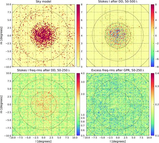
Top left-hand panel: Apparent NCP sky-model, convolved with a 7 arcmin FWHM Gaussian PSF, composed of more than 28 000 components distributed in 122 clusters. Top right-hand panel: 10 nights total intensity (Stokes I) image averaged over the 12 MHz bandwidth after DD calibration and sky-model subtraction, at 7 arcmin resolution. Bottom left-hand panel: 10 nights total intensity image rms along the frequency-direction, after DD calibration and sky-model subtraction, at 13 arcmin resolution. Bottom right-hand panel: 10 nights total intensity image rms along the frequency-direction after GPR residual foreground removal, at 13 arcmin resolution. All images are in units of Kelvin, and the three dashed circles indicate the approximate position of the primary beam nulls (≈4.5, 9, 13.5 deg).
Most likely the excess power is not due to just one of the above causes, but to a combination.
6.3 Future data-processing enhancements
Most of the causes of excess power that we discussed in the previous section could be mitigated by improving RFI mitigation, the instrumental and ionosphere calibration scheme, our sky model, and the GPR covariance model:
Improving the low level RFI flagging – Currently about 5 per cent of the uv-cells and several sub-bands are flagged after gridding. If this low-level RFI could be flagged on higher resolution data sets, this could improve our sensitivity and reduce their impact in the EoR window. Combining the time-differenced visibilities amplitude of all baselines, a technique recently introduced in Wilensky et al. (2019), will be used to identify faint RFI below the single baseline thermal noise. Ground-plan sources of broad-band RFI will also be investigated and suppressed using near-field imaging (e.g. Paciga et al. 2011).
Enforcing spectrally smooth solutions at the DI steps – This is not done right now and could still lead to small chromatic gain calibration errors. In this process, we will have to separately fit slowly time varying band-pass effects, such as cable reflections, which would not be modelled by the Bernstein polynomial prior. A second DI-calibration step with a long solution time and low regularization (i.e. bandpass calibration) would be able to solve them with limited extra noise (e.g. Barry et al. 2019; Li et al. 2019). We will also investigate directly using the Bernstein polynomial prior as gain solutions at the DI and DD steps which could reduce chromatic gain errors and the overfitting effect even further. This will also mitigate the impact of having an incomplete sky model (Barry et al. 2016; Ewall-Wice et al. 2017).
Improving the GPR covariance model – The GPR method requires a covariance model that is a good statistical description of the data to be effective. Covariance kernels that would better describe the foreground wedge and the 21 cm signal would improve this model. This requires building a physically motivated spectral and spatial covariance model for each source of mode-mixing contaminant (calibration errors, ionosphere, instrument chromaticity, ...) and building a 21 cm signal covariance model, directly parametrized with EoR physical parameters.
Optimizing sagecal calibration settings – We will also revise the solution times of the DD-calibration, the order of Bernstein polynomial prior and the maximum baselines used in the calibration. Decoupling the phase and amplitude solution time intervals could also further reduce calibration errors.
Improving the NCP sky model – Finally, a complete review of our current sky model will be carried out, investigating as well the inclusion of diffuse Stokes I, Q, and U emission as observed using the AARTFAAC21 HBA system (Prasad et al. 2016; Gehlot 2019).
7 CONCLUSIONS
The LOFAR-EoR KSP’s primary objective is to detect the 21 cm signal from the EoR in the redshift range z ≈ 7–11. We expect that a total of at least 1000 h of observation with the LOFAR-HBA system will be necessary for a detection of the signal predicated by a wide range of theoretical models (Mertens et al. 2018). Whereas in Patil et al. (2017) we presented a first upper limit from one night of data (13 h), in this work we processed twelve nights of data, combining the best ten nights (141 h). Compared to Patil et al. (2017), we have introduced significant enhancements in the direction-dependent calibration of the data, replaced the foregrounds mitigation strategy and improved the power spectra extraction, leading to significantly deeper limits on the 21 cm signal even when using the same data. Our main results are the following:
The excess power, due to gain overfitting (see Patil et al. 2016 for an extensive discussion), that appears on short baselines when a baseline cut is introduced between the imaging and calibration steps,22 has been considerably reduced by increasing (via regularization) the spectral smoothness of the gain solutions in the DD-calibration step. The ratio of the variance between adjacent sub-band differences and thermal noise power (based on visibility differences on a 10 s time scale) is reduced to a factor of ≈1.8 from a factor ≈10 in the procedure used in Patil et al. (2017). In addition, we introduced GPR (Mertens et al. 2018) to remove the residual foreground emission after sky-model subtraction in the DD-calibration step. We find GPR to be more suitable compared to the GMCA method (Chapman et al. 2013) in the implementation used by Patil et al. (2017).
We analysed data from twelve nights of observation obtained during LOFAR Cycles 0, 1, and 2. The data quality was found to be similar from night to night, except for two nights that were discarded from the final analysis. In all data sets, spectrally uncorrelated (white power spectrum) noise on baselines |$\lt \!100\, \lambda$| is larger than expected for thermal noise (by up to a factor 2 to 3). It is seen in both Stokes I and Stokes V, and does not appear to be related to the calibration, sky foregrounds, or polarization leakage, in any clear way. Low-level RFI, below the flagging threshold, could be a possible cause of this particular white excess noise on very short baselines. Further examination and mitigation of the excess noise is planned.
After foreground removal using both DD calibration and GPR, the Stokes I residual power spectrum is characterized by a spectrally correlated excess which is included in the overall GPR covariance model as a Matern kernel. It has a coherence scale lex ≈ 0.25–0.45 MHz, depending on the night. This excess is partially correlated between nights, especially in the foreground wedge region but also outside it. Larger correlations are also found between observations that started at similar LST times. The latter finding and the relatively rapid spectral de-correlation, together suggest that the residuals may originate from un-modelled or incorrectly modelled sky emission far from the phase centre.
After combining the best 10 out of 12 analysed nights of data (|$141\,{\rm h}$| of data), the residual Stokes I power decreased by a factor of ≈4 in the foreground wedge region, and by a factor of 5–6 outside of the wedge. The residuals are dominated by the same spectrally correlated excess noise found in all individual nights.
Based on the 141 h data set, we find an improved 2 − σ upper limit on the 21 cm signal power spectrum at z ≈ 9.1 of |$\Delta ^2_{21} \lt (72.86)^2\, \mathrm{mK^2}$| at |$k = 0.075 \mathrm{h\, cMpc^{-1}}$| (the lowest k-mode) and |$\Delta ^2_{21} \lt (106.65)^2\, \mathrm{mK^2}$| at |$k = 0.1 \mathrm{h\, cMpc^{-1}}$| (the reference k-mode), with a dk/k ≈ 0.3. The latter is an improvement by a factor ≈8 in power compared to the previous upper limit reported in Patil et al. (2017).
We have examined a range of possible origins for the excess power, including residual foregrounds emission from sources away from the phase centre, polarization leakage of Stokes Q and U emission to Stokes I, chromatic DI/DD-calibration errors and low-level RFI. No clear cause has yet been identified, but further improvements of our processing procedures are currently under way to reduce its level by (i) improving low-level RFI flagging, (ii) enforcing spectrally smooth solutions during DI-calibration, (iii) further optimizing sagecal calibration settings (regularization prior, number of ADMM iterations, applying the Bernstein polynomial prior itself instead of the regularized gain solutions), and (iv) using more physically motivated GPR covariance models that are not only defined in the frequency direction, but also in time and baseline, to better separate the various contributions to the power spectrum and 21 cm signal limits.
Based on current estimates of the thermal noise in the analysed data sets, which we believe to be accurate, and assuming that the excess power can be mitigated, one can reach a 2 − σ sensitivity limit of |$\approx \!(14)^2\, \mathrm{mK^2}$| at |$k = 0.1\, \mathrm{h\, cMpc^{-1}}$| from the same 10 nights of data, and a very deep |$\approx \!(4)^2\, \mathrm{mK^2}$| sensitivity limit, when combining about 100 nights of data, which is in the range where current 21 cm EoR models predict the power to be.
Although the cause of excess noise has still not been fully solved, the results presented in this paper are a significant step forward compared to those by Patil et al. (2017). Several issues that were identified in that work have now largely been mitigated, and a number of major improvements in our data processing procedure have been achieved. In the present analysis, possible sources of the excess power have been unveiled and solutions to mitigate them are currently investigated.
7.1 Implication of the upper limit on the EoR
The implications of the improved 21 cm signal power spectrum upper limit on the Epoch of Heating (EoH) and EoR are analysed in detail in an accompanying paper by Ghara et al. (2020) using the reionization simulation code grizzly (Ghara, Choudhury & Datta 2015; Ghara et al. 2018) and a Bayesian inference framework to constrain the parameters of the IGM. They study two sets of extreme scenarios that can be constrained by this upper limit: (i) For an IGM with a uniform spin temperature, they find that the models which can be ruled out have a combination of a very cold IGM (spin temperature |$\lt \!3\, \mathrm{K}$|) and a high UV photon emission rate (Ghara et al. 2020). (ii) In the case of a non-uniform IGM spin temperature, they find that the current upper limit is likely to rule out models with large emission regions which do not cover more than a third of an otherwise unheated IGM (Ghara et al. 2020).
ACKNOWLEDGEMENTS
FGM and LVEK would like to acknowledge support from a SKA-NL Roadmap grant from the Dutch Ministry of Education, Culture and Science. SZ acknowledges support from the Israeli Science Foundation (grant no. 255/18). ITI was supported by the Science and Technology Facilities Council (grants ST/I000976/1, ST/F002858/1, and ST/P000525/1); and The Southeast Physics Network (SEPNet). GM is thankful for support by Swedish Research Council grant 2016-03581. VJ acknowledges support by the Croatian Science Foundation for a project IP-2018-01-2889 (LowFreqCRO). EC acknowledges support from the Royal Society via. the Dorothy Hodgkin Fellowship.
Footnotes
Experiment to Detect the Global Epoch of Reionization Signature, https://loco.lab.asu.edu/edges/
Shaped Antenna measurement of the background RAdio Spectrum, http://www.rri.res.in/DISTORTION/saras.html
Low-Frequency Array, http://www.lofar.org
Murchison Widefield Array, http://www.mwatelescope.org
Precision Array to Probe EoR, http://eor.berkeley.edu
Giant Metrewave Radio Telescope, http://gmrt.ncra.tifr.res.in
Square Kilometre Array, http://www.skatelescope.org
Hydrogen Epoch of Reionization Array, http://reionization.org
The remote stations, which comprise nominally 48 tiles compared to the 24 tiles of a split core station, were tapered to have the same size and shape as the core stations.
Shapelets form an orthonormal basis in which a source of arbitrary shape can be described by a limited number of coefficients with sufficient accuracy (Yatawatta 2011).
All visibilities that go into one uv-cell are assumed to have the same noise and therefore the same weight.
This peculiar shape is explained by the fact that longer baselines (higher k⊥) change length more rapidly as a function of frequency than smaller baselines, causing increasingly faster spectral fluctuations, and thus producing power into proportionally higher |$k_{\parallel }$| modes.
Formally the chromatic nature of the instrument implies that mode-mixing has a multiplicative effect, but this can be approximated, to first order, as an additive effect, justifying the use of separable additive covariance for large and small frequency coherence scale foregrounds.
The primary beam and spatial tapering function introduce correlation, but those can be ignore at the scales we measure our power spectra: the width of the primary beam and tapering window is four times larger than the scale probed by our smallest baseline of |$50\, \lambda$|.
This is only done for illustration purposes, since the final result does not depend on the order in which the data are combined.
The smallest k bin in Patil et al. (2017) was |$0.053 \mathrm{h\, cMpc^{-1}}$|.
Amsterdam-ASTRON Radio Transients Facility and Analysis Center
That is, removing baselines |$\lt \!250\, \lambda$| during calibration and only imaging 50–250 λ baselines during the 21 cm signal analysis phase.
This procedure uses the emcee python package (http://dfm.io/emcee/current/) (Foreman-Mackey et al. 2013).
REFERENCES
APPENDIX A: SIGNAL INJECTION TESTS AND SIMULATIONS
GPR foreground mitigation may alter the 21 cm signal and assessing its efficiency and robustness is therefore crucial. In Mertens et al. (2018) we have carried out numerous tests against a large range of foregrounds simulations. Here we present tests which are more specifically connected to the frequency correlations observed in the LOFAR data.
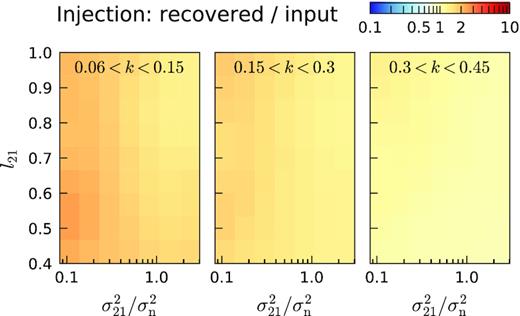
Result of the injection test for a wide range of coherence scale (l21) and S/N (|$\sigma ^2_{21} / \sigma ^2_{\mathrm{n}}$|) of the 21 cm like injected simulated signal. We plot the ratio of the recovered over injected signal spherically averaged power spectra for three k-bins.
Signal injection in simulated data – We also perform data simulations that reproduce the spectral correlations found in the full data set, using its optimal GPR covariance model parameters. For these simulations, our input ‘signal’ is the ‘21 cm signal’ and ‘excess’. GPR is applied to these data sets using a similar setup as for the injection tests, and we compute the ratio of the recovered over input power spectra. Our results (Fig. A2) show a ratio ≈1 for all the tested coherence scales and S/N of the 21 cm signal.
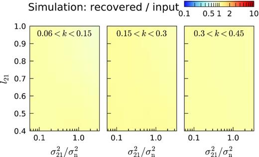
Result of the simulation test for a wide range of coherence scale l21 and S/N (|$\sigma ^2_{21} / \sigma ^2_{\mathrm{n}}$|) of the simulated 21 cm like signal. We plot the ratio of the recovered over injected signal spherically averaged power spectra for three k-bins. In this case, the recovered and input include the ‘excess’ signal.
APPENDIX B: CONFIDENCE INTERVAL ON THE GP MODEL HYPERPARAMETERS
An MCMC can be used to fully sample the posterior distribution of the GP model’s hyperparameters. This allows us to validate the optimal values obtained by optimization algorithm, and to estimate their confidence intervals. We apply the MCMC method23 described in Section 4.2.2 of Mertens et al. (2018) on the 10 nights data set. Fig. B1 shows the resulting posterior probability distribution of the GP model hyperparameters. The parameter estimates and confidence intervals are summarized in Table 3, along with their input values and associated priors. The correlation between the different parameters of the model is overall very small. All parameters are also well constrained, except the variance of the ‘21 cm signal’ component, which is consistent with zero.
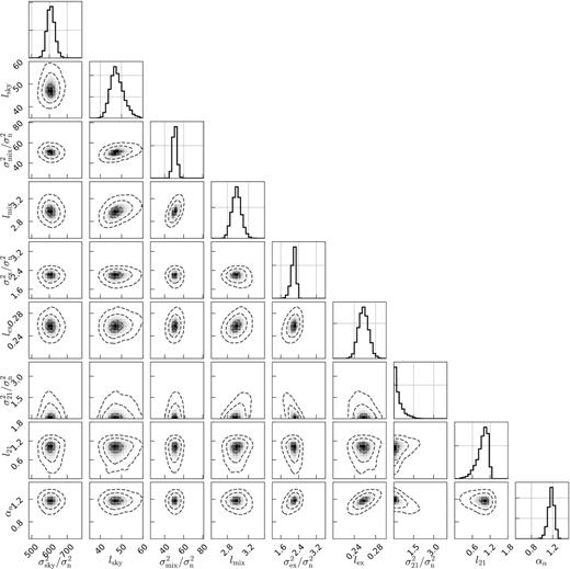
Posterior probability distributions of the GP model hyperparameters for the 10 nights data set. The covariance model has nine parameters: two for each of the sky, mix, 21, and ex (excess) components, plus the scaling factor αn. The black dashed contours show the 68 per cent, 95 per cent, and 99.7 per cent confidence interval.
