


ABSTRACT
Next generation interferometers, such as the Square Kilometre Array, are set to obtain vast quantities of information about the kinematics of cold gas in galaxies. Given the volume of data produced by such facilities astronomers will need fast, reliable, tools to informatively filter and classify incoming data in real time. In this paper, we use machine learning techniques with a hydrodynamical simulation training set to predict the kinematic behaviour of cold gas in galaxies and test these models on both simulated and real interferometric data. Using the power of a convolutional autoencoder we embed kinematic features, unattainable by the human eye or standard tools, into a 3D space and discriminate between disturbed and regularly rotating cold gas structures. Our simple binary classifier predicts the circularity of noiseless, simulated, galaxies with a recall of 85% and performs as expected on observational CO and H i velocity maps, with a heuristic accuracy of 95%. The model output exhibits predictable behaviour when varying the level of noise added to the input data and we are able to explain the roles of all dimensions of our mapped space. Our models also allow fast predictions of input galaxies’ position angles with a 1σ uncertainty range of ±17° to ±23° (for galaxies with inclinations of 82.5° to 32.5°, respectively), which may be useful for initial parametrization in kinematic modelling samplers. Machine learning models, such as the one outlined in this paper, may be adapted for SKA science usage in the near future.
1 INTRODUCTION
The age of Big Data is now upon us; with the Square Kilometre Array (SKA) and Large Synoptic Survey Telescope (LSST) both set to see first light in the mid-2020s.
A key area for big data in the next decades will be the studying of the kinematics of cold gas in galaxies beyond our own. This field will rely on interferometers, such as the SKA, thanks to their ability to reveal the morphology and kinematics of the cold gas at high spatial and spectral resolution. Current instruments like the Atacama Large Millimeter/submillimeter Array (ALMA) have revolutionized the study of gas in galaxies with their sensitive, high resolution, observations of gas kinematics. However, this field lacks the benefits afforded by fast survey instruments, having long been in an era of point and shoot astronomy. As such, large data sets capable of containing global statistics in this research domain have yet to emerge and studies are plagued by slow analytical methods with high user-involvement.
At the time of writing, large-scale radio interferometric surveys such as WALLABY (Duffy et al. 2012) and APERTIF (Oosterloo, Verheijen & van Cappellen 2010) are set to begin and will motivate the creation of tools that are scalable to survey requirements. However, these tools will be insufficient for screening objects come the advent of next-generation instruments which are set to receive enormous quantities of data, so large in fact that storing raw data becomes impossible.
In recent times, disc instabilities, feedback, and major/minor mergers have become favoured mechanisms for morphological evolution of galaxies (e.g. Parry, Eke & Frenk 2009; Bournaud et al. 2011; Sales et al. 2012), the effects of which are visible in their gas kinematics. Therefore, gas kinematics could be used to rapidly identify interesting structures and events suitable for understanding drivers of galaxy evolution (e.g. Diaz et al. 2019). If the kinematics of galaxies can accurately yield information on feedback processes and major/minor merger rates, then astronomers using next generation instruments could develop a better understanding of which mechanisms dominate changes in star formation properties and morphology of galaxies. In order to do this we must develop fast, robust, kinematic classifiers.
Recently, machine learning (ML) has been used successfully in astronomy for a range of tasks including gravitational wave detection (e.g. Shen et al. 2017; Zevin et al. 2017; Gabbard et al. 2018; George & Huerta 2018), exoplanet detection (e.g. Shallue & Vanderburg 2018), analysing photometric light-curve image sequences (e.g. Carrasco-Davis et al. 2019), and used extensively in studies of galaxies (e.g. Dieleman, Willett & Dambre 2015; Ackermann et al. 2018; Domínguez Sánchez et al. 2018a,b; Bekki 2019).
While using ML requires large data acquisition, training time, resources, and the possibility of results that are difficult to interpret, the advantages of using ML techniques over standard tools include (but are not limited to) increased test speed, higher empirical accuracy, and the removal of user-bias. These are all ideal qualities which suit tool-kits for tackling hyperlarge data sets. However, the use of ML on longer wavelength millimetre and radio galaxy sources has been absent, with the exception of a few test cases (e.g. Alger et al. 2018; Ma et al. 2018; Andrianomena, Rafieferantsoa & Davé 2019), with the use of such tests to study the gas kinematics of galaxies being non-existent. It is therefore possible that, in the age of big data, studying gas kinematics with ML could stand as a tool for improving interferometric survey pipelines and encouraging research into this field before the advent of the SKA.
Cold gas in galaxies that is unperturbed by environmental or internal effects will relax in a few dynamical times. In this state, the gas forms a flat disc, rotating in circular orbits about some centre of potential, to conserve angular momentum. Any disturbance to the gas causes a deviation from this relaxed state and can be observed in the galaxy’s kinematics. Ideally therefore, one would like to be able to determine the amount of kinetic energy of the gas invested in circular rotation (the so-called circularity of the gas; Sales et al. 2012). Unfortunately this cannot be done empirically from observations because an exact calculation of circularity requires full 6D information pertaining to the 3D positions and velocities of a galaxy’s constituent components. Instead, in the past, astronomers have used approaches such as radial and Fourier fitting routines (e.g. Krajnović et al. 2006a; Spekkens & Sellwood 2007; Bloom et al. 2017) or 2D power-spectrum analyses (e.g. Grand et al. 2015) to determine the kinematic regularity of gas velocity fields.
In this work we use an ML model, called a convolutional autoencoder, and a hydrodynamical simulation training set to predict the circularity of the cold interstellar medium in galaxies. We test our resulting model on both simulated test data and real interferometric observations. We use the power of convolutional neural networks to identify features unattainable by the human eye or standard tools and discriminate between levels of kinematic disorder of galaxies. With this in mind, we create a binary classifier to predict whether the cold gas in galaxies exhibit dispersion-dominated or disc-dominated rotation in order to maximize the recall of rare galaxies with disturbed cold gas.
In Section 1.1 we provide the necessary background information for understanding what ML models we use throughout this paper. In Section 2.1 we describe the measuring of kinematic regularity of gas in galaxies and how it motivates the use of ML in our work. In Section 2 we outline our preparation of simulated galaxies into a learnable training set as well as the ML methods used to predict corresponding gas kinematics. In Section 3 the results of the training process are presented and discussed with a variety of observational test cases. Finally, in Section 4 we explain our conclusions and propose further avenues of research.
1.1 Background to convolutional autoencoders
Convolutional neural networks (CNNs), originally named neocognitrons during their infancy (Fukushima 1980), are a special class of neural network (NN) used primarily for classifying multichannel input matrices, or images. Information is derived from raw pixels, negating the need for a user-involved feature extraction stage; the result being a hyperparametric model with high empirical accuracy. Today, they are used for a range of problems from medical imaging to driverless cars.
A conventional CNN can have any number of layers (and costly operations) including convolutions, max-pooling, activations, fully connected layers, and outputs and often utilize regularization techniques to reduce overfitting. (For a more in depth background to the internal operations of CNNs we refer the reader to Krizhevsky, Sutskever & Hinton 2012). These networks are only trainable (through back propagation) thanks to the use of modern graphics processing units (GPUs; Steinkraus, Buck & Simard 2005). It is because of access to technology such as GPUs that we are able to explore the use of ML in a preparatory fashion for instrument science with the SKA in this paper.
A CNN will train on data by minimizing the loss between sampled input images and a target variables. Should training require sampling from a very large data set, training on batches of inputs (also called mini-batches) can help speed up training times by averaging the loss between input and target over a larger sample of inputs. Should the network stagnate in minimizing the loss, reducing the learning rate can help the network explore a minimum over the parameter space of learnable weights and thus increase the training accuracy. Both of the aforementioned changes to the standard CNN training procedure are used in our models throughout this paper.
An autoencoder is a model composed of two subnets, an encoder and a decoder. Unlike a standard CNN, during training, an autoencoder learns to reduce the difference between input and output vectors rather than the difference between output vector and target label (whether this be a continuous or categorical set of target classes). In an undercomplete autoencoder the encoder subnet extracts features and reduces input images to a constrained number of nodes. This so-called bottleneck forces the network to embed useful information about the input images into a non-linear manifold from which the decoder subnet reconstructs the input images and is scored against the input image using a loss function. With this in mind, the autoencoder works similar to a powerful non-linear generalization of principal component analysis (PCA), but rather than attempting to find a lower dimensional hyperplane, the model finds a continuous non-linear latent surface on which the data best lies.
Autoencoders have been used, recently, in extragalactic astronomy for de-blending sources (Reiman & Göhre 2019) and image generation of active galactic nuclei (AGNs; Ma et al. 2018).
A convolutional autoencoder (CAE) is very similar to a standard autoencoder but the encoder is replaced with a CNN feature extraction subnet and the decoder is replaced with a transposed convolution subnet. This allows images to be passed to the CAE rather than 1D vectors and can help interpret extracted features through direct 2D visualization of the convolution filters. For an intuitive explanation of transposed convolutions we direct the reader to Dumoulin & Visin (2016) but for this paper we simply describe a transpose convolution as a reverse, one-to-many, convolution.
2 METHODOLOGY
2.1 Circularity parameter
As κ can only be calculated empirically from simulated galaxies, combining ML techniques with simulations will allow us to explore their abilities to learn features that can be used to recover κ in observations faster, and more robustly, than by human eye. In fact, κ has been used in previous studies to infer the origin of galaxy stellar morphologies (Sales et al. 2012) and, more recently, to investigate the kinematics of gas in post starburst galaxies (Davis et al. 2019).
2.2 EAGLE
The Evolution and Assembly of GaLaxies and their Environments (EAGLE) project1 is a collection of cosmological hydrodynamical simulations which follow the evolution of galaxies and black holes in a closed volume Λ cold dark matter (ΛCDM) universe. The simulations boast subgrid models which account for physical processes below a known resolution limit (Crain et al. 2015; Schaye et al. 2015; The EAGLE team 2017). These simulations are able to reproduce high levels of agreement with a range of galaxy properties which take place below their resolution limits (see e.g. Schaye et al. 2015). Each simulation was conducted using smooth particle hydrodynamics, meaning users can directly work with the simulated data in the form of particles, whose properties are stored in output files and a data base that can be queried.
In this paper we make use of these simulations, in conjunction with kinematic modelling tools, to generate a learnable training set. We then probe the use of this training set for transfer learning with the primary goal being to recover kinematic features from generated velocity maps. Using simulations has certain advantages over collecting real data including accessibility, larger sample sizes, and the ability to calculate empirical truths from the data. However, there are drawbacks, including: unproven model assumptions, imperfect physics, and trade-off between resolution and sample size due to computational constraints.
The scripts for reading in data, from the EAGLE project data base, were adapted versions of the EAGLE team’s pre-written scripts.2 The original simulations are saved into 29 snapshots for redshifts z = 0–20 and for this work we utilize snapshot 28 for RefL0025N0376 and RefL050N0752 and snapshots 28, 27, 26, and 25 for RefL0100N1504 (i.e. redshifts z = 0–0.27). When selecting galaxies from these snapshots, we set lower limits on the total gas mass (>1 × 10⁹ M⊙) and stellar mass (>5 × 10⁹ M⊙) within an aperture size of 30 kpc around each galaxy’s centre of potential (i.e. the position of the most bound particle considering all mass components), in order to exclude dwarf galaxies. In order to select particles which are representative of cold, dense, molecular gas capable of star formation, we only accepted particles with a SFR > 0 for pre-processing (as described in Section 2.3). There are many ways to select cold gas in the EAGLE simulations (Lagos et al. 2015) but we use this method for its simplicity as our primary goal is to create a model that is capable of learning low-level kinematic features so as to generalize well in transfer learning tests. The upper radial limit for particle selection of 30 kpc, from the centre of potential, is in keeping with the scales over which interferometers, such as ALMA, typically observe low-redshift galaxies. It is important that we replicate these scales in order to test our model performance with real data as described in Section 3.3. One should note that for future survey instruments, such as the SKA, an alternative scaling via consideration of noise thresholds would be more appropriate. However, as we are particularly interested in the performance of our models with ALMA observations, we instead impose a radial limit for this work. At this stage we also set a lower limit on the number of particles within the 30 kpc aperture to >200. This was to ensure we had enough particles to calculate statistically valid kinematic properties of the galaxies and reduce scaling issues caused by clipping pixels with low brightness when generating velocity maps. With these selection criteria, we work with a set of 14 846 simulated galaxies.
2.3 Data preparation
Each galaxy was rotated so that their total angular momentum vector was aligned with the positive z-axis using the centre of potential (as defined in the EAGLE Data base; see The EAGLE team 2017) as the origin. We then made use of the Python based kinematic simulator KinMS3 (KINematic Molecular Simulation) from Davis et al. (2013) to turn EAGLE data into mock interferometric observations. KinMS has flexibility in outputting astronomical data cubes (with position, position, and frequency dimensions) and moment maps from various physical parametrizations and has been used for CO molecular gas modelling in previous work (e.g. Davis et al. 2013) and for observational predictions from EAGLE (Davis et al. 2019). Using KinMS we generate simulated interferometric observations of galaxies directly from their 3D particle distributions.
Thanks to the controllable nature of the EAGLE data, we have the ability to generate millions of images from just a handful of simulations by using combinations of rotations and displacements of thousands of simulated galaxies per snapshot. This flexibility also has the added benefit of naturally introducing data augmentation for boosting the generalizing power of an ML algorithm. For any given distance projection, galaxies were given eight random integer rotations in position-angle (0° ≤ θpos < 360°) and inclination (5° ≤ ϕinc ≤ 85°). Each galaxy is displaced such that they fill a 64 arcsec × 64 arcsec mock velocity map image in order to closely reflect the field of view (FOV) when observing CO(1-0) line emission with ALMA. We define the displacement of each simulated galaxy in terms of their physical size and desired angular extent. Each galaxy’s radius is given as the 98th percentile particle distance from its centre of potential in kpc. We use this measurement, rather than the true maximum particle radius, to reduce the chance of selecting sparsely populated particles for calculating displacement distances, as they can artificially scale down galaxies.
The EAGLE galaxies were passed to KinMS to create cubes of stacked velocity maps, with fixed mock beam sizes of bmaj = 3 arcsec, ready for labelling. Each cube measured 64 × 64 × 8 where 64 × 64 corresponds to the image dimensions (in pixels) and eight corresponds to snapshots during position-angle and inclination rotations. The median physical scale covered by each pixel across all image cubes in a representative sample of our training set is 0.87 kpc. It should be noted that we set all non-numerical values or infinities to a constant value, as passing such values to an ML algorithm will break its training. We adopt 0 |$\rm{km\,s}^{-1}$| as our constant (similarly to Diaz et al. 2019) to minimize the background influencing feature extraction. Our training set has a range in blank fraction (i.e. the fraction of pixels in images with blank values set to 0 |$\rm{km\,s}^{-1}$|) of 0.14 to 0.98, with a median blank fraction of 0.52. Fig. 1 shows simulated ALMA observations of galaxies when using KinMS in conjunction with particle data from the EAGLE simulation RefL0025N0376.
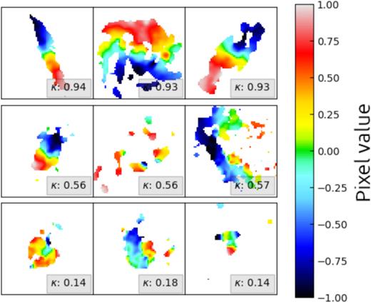
Random exemplar velocity maps for the noiseless EAGLE data set. Rows of increasing order, starting from the bottom of the figure, show galaxies of increasing κ. The κ for each galaxy is shown in the bottom right of the frame in a grey box. Each galaxy has randomly selected position angle and inclination and the colourbar indicates the line of sight velocities, which have been normalized into the range −1 to 1 and subsequently denoted as pixel values. The images have dimensions of 64 × 64 pixels in keeping with the size of input images to our models in this paper, as described in Section 2.6. One can easily see the changes in velocity field from κ ∼ 1 to κ ∼ 0 as galaxies appear less disc-like with more random velocities.
2.4 Simulating noise
Noise presents a problem when normalizing images into the preferred range. Rescaling, using velocities beyond the range of real values in a velocity map (i.e. scaling based on noise), will artificially scale down the true values and thus galaxies will appear to exhibit velocities characteristic of lower inclinations. We clip all noisy moment 1 maps at a fixed 96th percentile level, before normalizing, in order to combat this effect. Note that this choice of clipping at the 96th percentile level is arbitrarily based on a handful of test cases and represents no specific parameter optimization. Although simple, this likely reflects the conditions of a next generation survey in which clipping on the fly will be done using a predetermined method globally rather than optimizing on a case by case basis.
2.5 Labelling the training set
Each galaxy, and therefore every cube, is assigned a label in the continuous range of 0 to 1 corresponding to the level of ordered rotation, κ, of that galaxy.
In Fig. 1, the difference between levels of κ is clear in both structure and velocity characteristics, with low κ galaxies exhibiting less regular structures and more disturbed velocity fields than high κ galaxies.
Fig. 2 shows the distribution of κ in our training set. It is clear that our training set is heavily imbalanced with a bias towards the presence of high κ galaxies. Additionally, as κ approaches one, the possible variation in velocity fields decreases as there are limited ways in which one can create orderly rotating disc-like structures. However, our data set contains a surplus of galaxies as κ approaches one. Therefore, if one were to randomly sample from our data set, for training an ML model, then the model would undoubtedly overfit to high κ images. This is a common problem in ML particularly with outlier detection models whose objectives are to highlight the existence of rare occurrences. In Section 2.6 we describe our solution for this problem with the use of weighted sampling throughout training to balance the number of galaxies with underrepresented κ values seen at each training epoch.
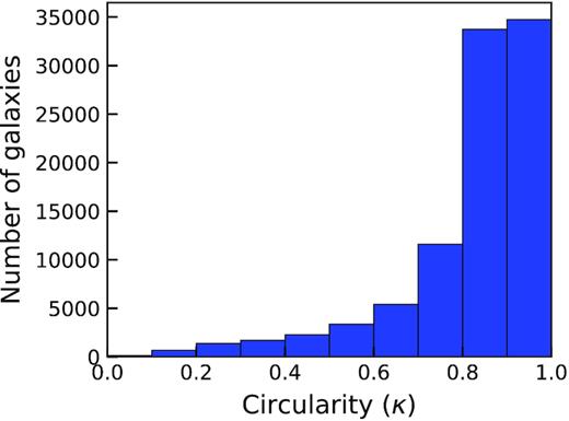
A histogram of κ labelled galaxies in the noiseless EAGLE training set. Galaxies have been binned in steps of δκ = 0.1 for visualization purposes but remain continuous throughout training and testing. The distribution of κ is heavily imbalanced, showing that more galaxies exhibit a κ closer to 1 than 0.
2.6 Model training: Rotationally invariant case
In this section we describe the creation and training of a convolutional autoencoder to embed κ into latent space and build a binary classifier to separate galaxies with κ above and below 0.5. Note that 0.5 is an arbitrarily chosen threshold for our classification boundary but is motivated by the notion of separating ordered from disturbed gas structures in galaxies.
In order to construct our ML model, we make use of PyTorch4 0.4.1, an open source ML library capable of GPU accelerated tensor computation and automatic differentiation (Paszke et al. 2017). Being grounded in Python, PyTorch is designed to be linear and intuitive for researchers with a C99 API backend for competitive computation speeds. We use PyTorch due to its flexible and user friendly nature for native Python users.
A visual illustration of the CAE architecture is shown in Fig. 3 and described in Table A1 in more detail. The model follows no hard structural rules and is an adaption of standard CNN models. The decoder structure is simply a reflection of the encoder for simplicity. This means our CAE is unlikely to have the most optimized architecture and we propose this as a possible avenue for improving on the work presented in this paper. The code developed for this paper is available on GitHub5 as well as an ongoing development version.6
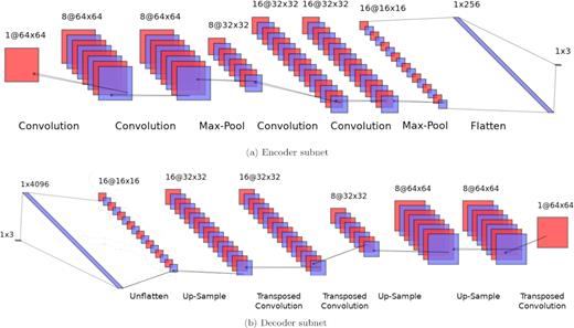
Illustration of the CAE architecture used in this paper. The encoder subnet (top) makes use of a series of convolutions and max-pooling operations to embed input image information into three latent dimensions. The decoder subnet (bottom) recovers the input image using transposed convolutions and up-sampling layers. The output of the encoder is passed to the decoder during training but throughout testing only the encoder is used map velocity maps into latent space.
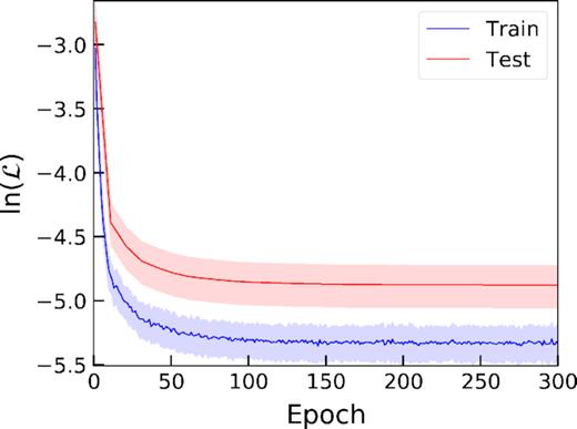
Training the CAE on noiseless EAGLE velocity maps. The solid lines show the natural log mean MSE loss and solid colour regions show 1σ spread at any given epoch. In order to reduce computational time, the test accuracy is evaluated every 10th epoch. We see smooth convergence of our CAE throughout training with no turnover of the test accuracy indicating that our model did not overfit to the training data.
The CAE learned to encode input images to 3D latent vectors. Further testing showed that any higher compression, to lower dimensions, resulted in poor performance for the analyses described in Section 3 and compression to higher dimensions impaired our ability to directly observe correlations between features and latent positions with no improvement to the model’s performance. We use scikit-learn’s7 PCA function on these vectors to rotate the latent space so that it aligns with one dominant latent axis, in this case the z axis. As seen in Fig. 5, the 3D latent space contains structural symmetries which are not needed when attempting to recover κ (but are still astrophysically useful; see Section 3.5). Because of this, the data are folded around the z and x axes consecutively to leave a 2D latent space devoid of structural symmetries with dimensions |z| and |$\sqrt{x^{2}+y^{2}}$| from which we could build our classifier (see Section 3.3).
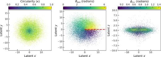
Noiseless eagle test data in 3D latent space. All subplots show the same latent structure but coloured differently by: true κ (left), true position angle (θpos, middle), and true inclination (ϕinc, right). It is clear from the right subplot that low κ galaxies lie close to the z = 0 region. θpos is very neatly encoded in the clockwise angle around the latent z-axis. The red dashed line indicates the positive latent x axis from which θpos is measured. ϕinc appears to be encoded in a much more complex fashion than κ and θpos.
Having tested multiple classifiers on the 2D latent space (such as high-order polynomial and regional boundary approaches), we find that a simple vertical boundary line is best at separating the galaxies whose κ are greater than or less than 0.5. This is highlighted in Fig. 6, where we see the spread on latent positions taken up by different κ galaxies makes a regression to recover κ too difficult. In order to optimize the boundary line location, we measure the true positive (TP), true negative (TN), false positive (FP), and false negative (FN) scores when progressively increasing the boundary line’s x location. The intersection of TP and TN lines (and therefore the FP and FN lines) in Fig. 7 indicates the optimal position for our boundary, which is at |$\sqrt{x^{2}+y^{2}}=2.961\pm 0.002$|. The smoothness of the lines in Fig. 7 show how the two κ populations are well structured. If the two populations were clumpy and overlapping, one would observe unstable lines as the ratio of positive and negatively labelled galaxies constantly shifts in an unpredictable manner.
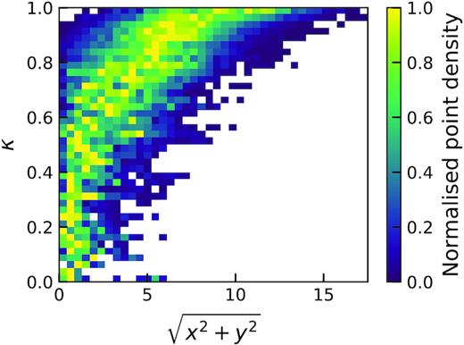
2D histogram of κ against latent position for noiseless EAGLE test data. Pixels are coloured by point density normalized such that the point density in each row lies in the range 0 to 1. We see a very clear relationship between κ and latent position but also a high spread of latent positions occupied by high κ galaxies, making a regression task to recover κ from our encoding difficult.
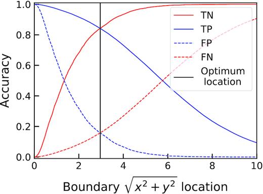
The observed change in all four components of a confusion matrix when changing the boundary line x-location. The optimal position for a binary classification is chosen as the intersection of TP and TN lines, which is identical to the location at the intersection of FP and FN lines. We observe smooth changes to the TN, TP, FP, and FN lines as the boundary line location changes, showing that both target populations are well clustered.
3 RESULTS AND DISCUSSION
3.1 Test case I: Noiseless EAGLE data
The number of high and low κ labelled images, in both the training and test sets, for the noiseless EAGLE data set are shown in Table 1. Fig. 8(a) shows the classification accuracy on the noiseless EAGLE training set. The TP and TN accuracy scores are unsurprisingly identical given the method used to find the optimal boundary in Section 2.6 was designed to achieve this (see intersection points in Fig. 7). The classifier has a mean training recall of 84 % for both classes.
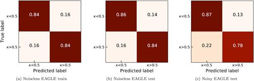
Normalized confusion matrix showing the performance of the classifier when testing the 8(a) noiseless EAGLE training set, 8(b) noiseless EAGLE test set (seeded with Gaussian noise with |$\frac{1}{\text{S/N}} = \frac{1}{10}$| and masking at three times the RMS level of line free regions), and 8(c) noisy EAGLE test set. The mean recall scores are 84 %, 85 %, and 82.5 %, respectively.
Proportions of high and low κ labelled images in both training and test sets for the noiseless EAGLE data set.
| Number of images | |||
|---|---|---|---|
| Data set | κ > 0.5 | κ < 0.5 | Total |
| Training | 88 840 (94 %) | 6144 (6 %) | 94 984 |
| Test | 22 224 (93 %) | 1560 (7 %) | 23 784 |
| Number of images | |||
|---|---|---|---|
| Data set | κ > 0.5 | κ < 0.5 | Total |
| Training | 88 840 (94 %) | 6144 (6 %) | 94 984 |
| Test | 22 224 (93 %) | 1560 (7 %) | 23 784 |
Fig. 8(b) shows the confusion matrix when testing the noiseless EAGLE test set using our boundary classifier. We see that the model performs slightly better than when tested on the training set, suggesting that the model did not overfit to the training data and is still able to encode information on κ for unseen images.
3.2 Test case II: Noisy EAGLE data
Fig. 8(c) shows the results of classifying noisy EAGLE test data with S/N = 10 and masking at three times the RMS level (see Section 2.4 for details). Note that this is a simple test case and places no major significance on the particular level of S/N used. The introduction of noise has a clear and logical, yet arguably minor, impact on the classifier’s accuracy. The combination of adding noise followed by using an arbitrary clipping level causes test objects to gravitate towards the low κ region in latent space. This should come as no surprise as κ correlates with ordered motion; therefore, any left over noise from the clipping procedure, which itself appears as disorderly motions and structures in velocity maps, anticorrelates with κ causing a systematic shift towards the low κ region in latent space.
One could reduce this shifting to low κ regions in several ways. (1) Removing low S/N galaxies from the classification sample. (2) For our test cases we used a single absolute percentile level for smooth clipping noise; using levels optimized for cases on a one-by-one basis will prevent overclipping. (3) If one were to directly sample the noise properties from a specific instrument, seeding the simulated training data with this noise before retraining an CAE would cause a systematic shift in the boundary line, mitigating a loss in accuracy. It should also be noted that we have not tested the lower limit of S/N for which it is appropriate to use our classifier but instead we focus on demonstrating the effects of applying noise clipping globally across our test set under the influence of modest noise.
3.3 Test case III: ALMA data
We tested 30 velocity maps of galaxies observed with ALMA to evaluate the performance of the classifier on real observations. Given that we used KinMS to tailor the simulated velocity maps to closely resemble observations with ALMA we expect similar behaviour as seen when testing the simulated data. For our test sample we use an aggregated selection of 15 velocity maps from the mm-Wave Interferometric Survey of Dark Object Masses (WISDOM) CO(1-0, 2-1, and 3-2) and 15 CO(1-0) velocity maps from the ALMA Fornax Cluster Survey (AlFoCS; Zabel et al. 2019). We classify each galaxy, by eye, as either disturbed or regularly rotating (see Table A2) in order to heuristically evaluate the classifier’s performance.
Fig. 9 shows the positions of all ALMA galaxies (round markers) in our folded latent space, once passed through the CAE. Of the 30 galaxies, 6 (20 %) are classified as κ < 0.5; this higher fraction, when compared to the fraction of low κ galaxies in the simulated test set, is likely due to the high number of dwarf galaxies, with irregular H2 gas, targeted in AlFoCS.

Folded latent space positions of noiseless EAGLE galaxies (coloured 2D histogram), ALMA galaxies (circular markers), and LVHIS galaxies (triangular markers); the suspected low κ galaxies are coloured red and suspected high κ galaxies coloured blue. The EAGLE points are coloured by average value of κ in each 2D bin and the grey dashed line shows the classifier boundary between κ < 0.5 and κ > 0.5 objects. Eight of the 10 suspected low κ LVHIS galaxies are classified as κ < 0.5 and five of the seven suspected low κ ALMA galaxies are classified as κ < 0.5. In both cases we see only one misclassification far from the boundary line and low κ region. A selection of three LVHIS and three ALMA galaxies are shown to the left and right of the central plot, respectively, their locations in latent space indicated by black numbers. Images are scaled to 64 × 64 pixels with values normalized between −1 to 1, because of this images are shown as a close representation of CAE inputs before latent encoding. For illustration purposes the backgrounds have been set to nan whereas the CAE would instead see these regions as having a value of 0.
We find one false positive classification close to the classification boundary and one false positive classification far from the classification boundary. The false negative classification of NGC 1351A can be explained by its disconnected structure and edge-on orientation (see Zabel et al. 2019; fig. B1). Since low κ objects appear disconnected and widely distributed among their velocity map fields of view, it is understandable why NGC 1351A has been misclassified as a disturbed object. It should be noted that upon inspection the false positive classification of FCC282 can be attributed to the appearance of marginal rotation in the galaxy. We see evidence of patchy high κ galaxies residing closer to the classification boundary than non-patchy examples. This may indicate a relationship between patchiness and latent positioning. The classifier performs with an accuracy of 90 % when compared to the predictions by human eye. Of the 30 galaxies observed with ALMA, 6 (20 %) are classified as low κ and of the 23 (77 %) galaxies identified by eye as likely to be high κ galaxies, only one was misclassified as low κ.
3.4 Test case IV: LVHIS data
In order to test the robust nature of the classifier, we used it to classify velocity maps of H i velocity fields from the Local Volume HI Survey (LVHIS; Koribalski et al. 2018). This is an important test as it determines the applicability of the classifier to H i line emission observations, the same emission that the SKA will observe. As described in Section 2.3, the EAGLE training set was designed to reflect observations with ALMA, making this transfer learning test a good opportunity to evaluate the model’s ability to generalize to unseen data containing different systematic characteristics.
Rather than moment masking the data cubes, like in Section 3.2, each cube is clipped at some fraction of the RMS (calculated in line free channels) to mimic the noise removal processes used in generating velocity maps in the LVHIS data base. All galaxies whose positions could not be found using the Python package astroquery8 (searching the SIMBAD Astronomical Data base9), or whose H i structures were clearly misaligned with the true galaxy centres, were omitted from further testing. This was to prevent misclassification based on pointing error which correlates with features of disorderly rotation to the CAE and would artificially increase the FN rate. This left 61 galaxies (see Table A3) from which velocity maps were made and passed through the CAE. Finally, where images were not 64 × 64 pixels, we used PyTorch’s torch.nn.functional.interpolation function (in bilinear mode) to rescale them up or down to the required dimensions prior to clipping.
The latent positions of all H i galaxies are shown in Fig. 9 (triangular markers). Of the 61 galaxies, 8 (13 %) are classified as low κ. By eye, we identified 10 galaxies in the LVHIS which are likely to be definitively classified as κ < 0.5 (see Table A3). Of these 10 candidates, eight were correctly identified as κ < 0.5, one is observed as very close to the classification boundary, and one is unquestionably misclassified.
3.5 Recovering position angle
Scientists who wish to model the kinematics of galaxies often require initial estimates for parameters such as position angle, inclination, mass components, radial velocity profiles etc. Given that position angle is clearly encoded in our latent xy plane (see Fig. 5), it is possible to return predicted position angles with associated errors. This could prove useful for fast initial estimates of θpos for scientists requiring them for kinematic modelling. We define the predicted position angle, θlatent, as the clockwise angle between the positive latent x-axis and the position of data points in the latent xy plane. We removed the systematic angular offset, δθ, between the positive latent x-axis and the true position angle (θpos) =0° line by rotating the latent positions by the median offset, found to be δθ ∼ 36.6°, and subtracting an additional 180°. In the now rotated frame, θlatent is defined as |$\tan ^{-1}\left(\frac{y}{x}\right)$|, where x and y are the latent x and y positions of each galaxy (see Fig. 10). We calculated errors on the resulting predictions of θlatent by taking the standard deviation of residuals between θlatent and θpos.
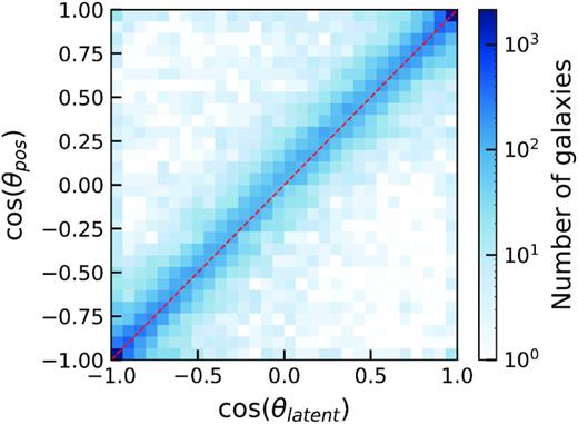
2D histogram showing the predicted position angles for the noiseless EAGLE test set against their true position angles. The red dashed line shows the 1:1 line along which all data would lie for a perfect predictor of position angle.
We repeated this procedure for the noisy EAGLE data, with S/N = 10, the results of which are also shown in Fig. 11 with red error bars. We can see that the recovery of θpos is still well constrained at higher inclinations with only a slight increase in the error most notably at lower inclinations (see Fig. 11. We see that at higher inclinations the error in predicted θpos is better constrained than for lower inclinations. This should come as no surprise as the ellipticity of galaxies and the characteristic shape of their isovels are gradually lost as a galaxy approaches lower inclinations thus making it more difficult to calculate θpos. During further testing we also observe reduced errors on position angles when limiting to higher κ test galaxies.
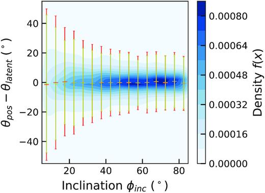
Kernel density estimation of error in θpos against inclination for noiseless EAGLE test data (yellow error bars) and noisy EAGLE test data (red error bars). Coloured contours show the 2D probability density, central horizontal line markers show the mean error in θpos in bins of width δθpos = 5°. The error bars show the standard error in each bin.
It should be noted that our method for recovering θpos is not the only one. Other kinematic fitting routines exist for this purpose including fit_kinematic_pa (Krajnović et al. 2006b) and the radon transform method (Stark et al. 2018). These methods likely have higher accuracy than seen here, as our network was not optimized for the recovery of θpos. Bench marking an ML model against existing ones, as a dedicated standalone mechanism for recovering θpos, is an avenue for future research.
Given that there is such a strong overlap in z-positions occupied by different galaxy inclinations, we were unable to recover the inclinations of galaxies in the simple manner as for θpos. However, from visualization the distribution of inclinations against latent-z position, we are confident that inclination plays a part in latent positioning of galaxies. Because of this we are confident in our understanding of all three latent dimensions that the CAE has learned.
4 CONCLUSIONS
We have shown that it is possible to use ML to encode high dimensional (64 × 64 pixels) velocity maps into three dimensions, while retaining information on galaxy kinematics, using convolutional autoencoders. We have successfully recovered the level of ordered rotation of galaxies using a simple binary classifier, from a multitude of test sets including simulated EAGLE velocity maps, ALMA velocity maps, and H i survey velocity maps. When testing real observational data, we see a clustering of low κ galaxies towards the origin and around the classification boundary, in line with our understanding of our folded 2D latent space. Our tests on simulated data show a mean recall of 85 % when attempting to recover the circularity parameter as well as 90 % and 97 % heuristic accuracy when recovering the circularity parameter for galaxies observed with ALMA and as part of LVHIS, respectively. We have managed to mitigate the problems associated with a heavily imbalanced training set by using both weighted sampling during training and balancing the true positive and true negative accuracy scores when constructing our classifier. In addition to recovering information on the ordered rotation characteristics of galaxies, we have also been successful in providing estimates on position angle from the full 3D latent positions of velocity maps with associated errors. These will be useful for initial guesses at θpos for kinematic modelling routines in related work.
We were able to show our classifier’s positive performance when testing LVHIS data. This outcome is important for two reasons: (1) it shows the robustness of the classifier when making the transition from simulated to real data of different origins and (2) it shows that using machine learning to study the kinematics of H i sources is likely possible and therefore applicable to SKA science.
Recovering inclinations, ϕinc, of galaxies was not possible using our CAE due to the high overlap in latent z positions for the entire range of ϕinc. However, the spread of z positions occupied by galaxies at mid-range inclinations was considerably less than at lower inclinations, indicating that while ϕinc is not recoverable, we are confident that it is partly responsible for the positions of galaxies in the latent z-axis. Therefore, we have a rational understanding of what information all three latent dimensions are encoding from the input images. This makes our model predictable and logical in how it behaves when seeing input data. This understanding is often missing in CNN style networks, and especially in deep learning models.
The main caveat with this work pertains to the use of percentages in our maximum-likelihood function when calculating the optimal boundary line for the binary classifier. This makes our classifier independent of the underlying distribution of high and low κ galaxies in an attempt to maximize the recall of both classes. The means our classifier will work well in situations where both classes are more equally distributed (such as galaxy clusters). However, one should take care when testing heavily imbalanced data sets where, although the data set has been drastically thinned of high κ galaxies, it is likely that the user will still need to examine the low κ classification set for contaminants.
As demonstrated by Diaz et al. (2019), using a combination of morphology and kinematics for classification purposes improves performance over using only one attribute. Therefore, a logical improvement on our work would be using a branched network or an ensemble of networks which use both moment zero and moment one maps to make predictions on kinematic properties. Our models rely on using maps of galaxies which are centred on their centres of potential (i.e. the position of the most bound particle); therefore, our classifier is sensitive to the choice of centre of potential proxy. This is undeniably an issue for on-the-fly surveys where the centre of potential of a target is estimated rather than empirically calculable. Therefore, including information such as intensity maps may allow re-centring based on observed characteristics rather than archived pointings for improving the classifiers performance. We see this as the most lucrative avenue for improving our models in the future.
Performing operations on a velocity map, as we have done in this work, means we are working several levels of abstraction away from the raw data cubes that future instruments, such as the SKA, will create. Therefore improvements could be made on our methods to analyse the effects of encoding data cubes into latent space rather than velocity maps. CNNs have long been capable of performing operations on multichannel images, making this avenue of research possible and useful in reducing the need for heavy processing of raw data cubes before processing with ML algorithms as we have done in the work.
ACKNOWLEDGEMENTS
The authors would like to thank the anonymous reviewer for their useful comments which improved this manuscript.
This paper has received funding by the Science and Technology Facilities Council (STFC) as part of the Cardiff, Swansea & Bristol Centre for Doctoral Training.
We gratefully acknowledge the support of NVIDIA Corporation with the donation of a Titan Xp GPU used for this research.
This research made use of astropy,10 a community-developed Python package for Astronomy (Astropy Collaboration 2013, 2018).
This paper makes use of the following ALMA data:
ADS/JAO.ALMA#2013.1.00493.S ADS/JAO.ALMA#2015.1.00086.S ADS/JAO.ALMA#2015.1.00419.S ADS/JAO.ALMA#2015.1.00466.S ADS/JAO.ALMA#2015.1.00598.S ADS/JAO.ALMA#2016.1.00437.S ADS/JAO.ALMA#2016.1.00839.S ADS/JAO.ALMA#2015.1.01135.S ADS/JAO.ALMA#2016.1.01553.S ADS/JAO.ALMA#2016.2.00046.S
ALMA is a partnership of the ESO (representing its member states), NSF (USA), and NINS (Japan), together with the NRC (Canada), NSC, ASIAA (Taiwan), and KASI (Republic of Korea), in cooperation with the Republic of Chile. The Joint ALMA Observatory is operated by the ESO, AUI/NRAO, and NAOJ.
JD wishes to thank Dr. Freeke van de Voort, from the Max Planck Institute for Astrophysics, for her help in querying the EAGLE data base and understanding the circularity parameter used throughout this paper.
We thank the PyTorch community for their assistance in learning the ropes of implementing and training neural networks with PyTorch. PyTorch is an optimized, open source, tensor library for deep learning using GPUs and CPUs.
Footnotes
REFERENCES
APPENDIX A: INFORMATION ON TEST GALAXIES
Architecture for our autoencoder, featuring both encoder and decoder subnets. The decoder is a direct reflection of the encoder’s structure.
| Layer | Layer type | Units/number of filters | Size | Padding | Stride | |
|---|---|---|---|---|---|---|
| Encoder | Input | Input | – | (64,64) | – | – |
| Conv1 | Convolutional | 8 | (3,3) | 1 | 1 | |
| ReLU | Activation | – | – | – | – | |
| Conv2 | Convolutional | 8 | (3,3) | 1 | 1 | |
| ReLU | Activation | – | – | – | – | |
| MaxPool | Max-pooling | – | (2,2) | – | 1 | |
| Conv3 | Convolutional | 16 | (3,3) | 1 | 1 | |
| ReLU | Activation | – | – | – | – | |
| Conv4 | Convolutional | 16 | (3,3) | 1 | 1 | |
| ReLU | Activation | – | – | – | – | |
| MaxPool | Max-pooling | – | (2,2) | – | 1 | |
| Linear | Fully-connected | 3 | – | – | – | |
| Decoder | Linear | Fully-connected | 3 | – | – | – |
| Up | Partial inverse max-pool | – | (2,2) | – | 1 | |
| ReLU | Activation | – | – | – | – | |
| Trans1 | Transposed Convolution | 16 | (3,3) | 1 | 1 | |
| ReLU | Activation | – | – | – | – | |
| Trans2 | Transposed Convolution | 16 | (3,3) | 1 | 1 | |
| Up | Partial inverse max-pool | – | (2,2) | – | 1 | |
| ReLU | Activation | – | – | – | – | |
| Trans3 | Transposed Convolution | 8 | (3,3) | 1 | 1 | |
| ReLU | Activation | – | – | – | – | |
| Trans4 | Transposed Convolution | 8 | (3,3) | 1 | 1 | |
| Ouput | Output | – | (64,64) | – | – |
ALMA galaxies selected from the WISDOM and AlFoCS surveys. WISDOM targets have beam major axes ranging from 2.4 to 6.7 arcsec with a mean of 4.4 arcsec and pixels/beam values ranging from 2.42 to 6.68 with a median value of 4.46. ALL WISDOM targets have channel widths of 2 |$\rm{km\,s}^{-1}$| bar one target which has a channel width of 3 |$\rm{km\,s}^{-1}$|. AlFoCS targets have beam major axes ranging from 2.4 to 3.3 arcsec with a mean of 2.9 arcsec and pixels/beam values ranging from 5.25 to 7.85 with a median value of 6.46. AlFoCS targets have channel widths ranging from 9.5 to 940 |$\rm{km\,s}^{-1}$|, with a median channel width of 50 |$\rm{km\,s}^{-1}$|. Of all 30 galaxies in the test set, seven were identified by eye as most likely to be classified as κ < 0.5 and their associated model predictions are shown. 27 (90 percent) of the galaxies are classified as predicted by human eye. NGC 1351A is the only false negative classification owing to its disconnected structure and edge on orientation.
| Object ID | Survey | Author prediction | Model prediction | Heuristic result |
|---|---|---|---|---|
| (disturbed=0, regular = 1) | (κ < 0.5 = 0, κ > 0.5 = 1) | (TP=true positive, FP = false positive TN=true negative, FN = false negative) | ||
| ESO358-G063 | AlFoCS | 1 | 1 | TP |
| ESO359-G002 | AlFoCS | 0 | 0 | TN |
| FCC207 | AlFoCS | 1 | 1 | TP |
| FCC261 | AlFoCS | 0 | 0 | TN |
| FCC282 | AlFoCS | 0 | 1 | FP |
| FCC332 | AlFoCS | 0 | 0 | TN |
| MCG-06-08-024 | AlFoCS | 0 | 0 | TN |
| NGC 1351A | AlFoCS | 1 | 0 | TN |
| NGC 1365 | AlFoCS | 1 | 1 | TP |
| NGC 1380 | AlFoCS | 1 | 1 | TP |
| NGC 1386 | AlFoCS | 1 | 1 | TP |
| NGC 1387 | AlFoCS | 1 | 1 | TP |
| NGC 1436 | AlFoCS | 1 | 1 | TP |
| NGC 1437B | AlFoCS | 1 | 1 | TP |
| PGC013571 | AlFoCS | 0 | 1 | FP |
| NGC 0383 | WISDOM | 1 | 1 | TP |
| NGC 0404 | WISDOM | 0 | 0 | TN |
| NGC 0449 | WISDOM | 1 | 1 | TP |
| NGC 0524 | WISDOM | 1 | 1 | TP |
| NGC 0612 | WISDOM | 1 | 1 | TP |
| NGC 1194 | WISDOM | 1 | 1 | TP |
| NGC 1574 | WISDOM | 1 | 1 | TP |
| NGC 3368 | WISDOM | 1 | 1 | TP |
| NGC 3393 | WISDOM | 1 | 1 | TP |
| NGC 4429 | WISDOM | 1 | 1 | TP |
| NGC 4501 | WISDOM | 1 | 1 | TP |
| NGC 4697 | WISDOM | 1 | 1 | TP |
| NGC 4826 | WISDOM | 1 | 1 | TP |
| NGC 5064 | WISDOM | 1 | 1 | TP |
| NGC 7052 | WISDOM | 1 | 1 | TP |
LVHIS galaxies chosen from the LVHIS data base as suitable for testing. The targets have beam major axes ranging from 5.3 to 34.7 arcsec with a mean of 13.2 arcsec and have pixels/beam values ranging from 5.25 to 34.74 with a median value of 12.78. The channel widths are 4 |$\rm{km\,s}^{-1}$| bar one target which has a channel width of 8 |$\rm{km\,s}^{-1}$|. Of all 61 galaxies in the test set, 10 (16 percent) were identified by eye as most likely to be classified as κ < 0.5 and their associated model predictions are shown. Of these 10 galaxies eight were correctly identified as low κ by the binary classifier with no false negative predictions.
| LVHIS ID | Object ID | Author prediction | Model prediction | Heuristic result |
|---|---|---|---|---|
| (disturbed=0, regular = 1) | (κ < 0.5=0, κ > 0.5 = 1) | (TP=true positive, FP = false positive TN=true negative, FN = false negative) | ||
| LVHIS 001 | ESO 349-G031 | 1 | 1 | TP |
| LVHIS 003 | ESO 410-G005 | 0 | 1 | FP |
| LVHIS 004 | NGC 55 | 1 | 1 | TP |
| LVHIS 005 | NGC 300 | 1 | 1 | TP |
| LVHIS 007 | NGC 247 | 1 | 1 | TP |
| LVHIS 008 | NGC 625 | 1 | 1 | TP |
| LVHIS 009 | ESO 245-G005 | 1 | 1 | TP |
| LVHIS 010 | ESO 245-G007 | 0 | 0 | TN |
| LVHIS 011 | ESO 115-G021 | 1 | 1 | TP |
| LVHIS 012 | ESO 154-G023 | 1 | 1 | TP |
| LVHIS 013 | ESO 199-G007 | 1 | 1 | TP |
| LVHIS 015 | NGC 1311 | 1 | 1 | TP |
| LVHIS 017 | IC 1959 | 1 | 1 | TP |
| LVHIS 018 | NGC 1705 | 1 | 1 | TP |
| LVHIS 019 | ESO 252-IG001 | 1 | 1 | TP |
| LVHIS 020 | ESO 364-G?029 | 1 | 1 | TP |
| LVHIS 021 | AM 0605-341 | 1 | 1 | TP |
| LVHIS 022 | NGC 2188 | 1 | 1 | TP |
| LVHIS 023 | ESO 121-G020 | 1 | 1 | TP |
| LVHIS 024 | ESO 308-G022 | 1 | 1 | TP |
| LVHIS 025 | AM 0704-582 | 1 | 1 | TP |
| LVHIS 026 | ESO 059-G001 | 1 | 1 | TP |
| LVHIS 027 | NGC 2915 | 1 | 1 | TP |
| LVHIS 028 | ESO 376-G016 | 1 | 1 | TP |
| LVHIS 029 | ESO 318-G013 | 1 | 1 | TP |
| LVHIS 030 | ESO 215-G?009 | 1 | 1 | TP |
| LVHIS 031 | NGC 3621 | 1 | 1 | TP |
| LVHIS 034 | ESO 320-G014 | 1 | 1 | TP |
| LVHIS 035 | ESO 379-G007 | 1 | 1 | TP |
| LVHIS 036 | ESO 379-G024 | 0 | 0 | TN |
| LVHIS 037 | ESO 321-G014 | 1 | 1 | TP |
| LVHIS 039 | ESO 381-G018 | 1 | 1 | TP |
| LVHIS 043 | NGC 4945 | 1 | 1 | TP |
| LVHIS 044 | ESO 269-G058 | 1 | 1 | TP |
| LVHIS 046 | NGC 5102 | 1 | 1 | TP |
| LVHIS 047 | AM 1321-304 | 0 | 0 | TN |
| LVHIS 049 | IC 4247 | 0 | 1 | FP |
| LVHIS 050 | ESO 324-G024 | 1 | 1 | TP |
| LVHIS 051 | ESO 270-G017 | 1 | 1 | TP |
| LVHIS 053 | NGC 5236 | 1 | 1 | TP |
| LVHIS 055 | NGC 5237 | 1 | 1 | TP |
| LVHIS 056 | ESO 444-G084 | 1 | 1 | TP |
| LVHIS 057 | NGC 5253 | 0 | 0 | TP |
| LVHIS 058 | IC 4316 | 0 | 0 | TP |
| LVHIS 060 | ESO 325-G?011 | 1 | 1 | TP |
| LVHIS 063 | ESO 383-G087 | 0 | 0 | TN |
| LVHIS 065 | NGC 5408 | 1 | 1 | TP |
| LVHIS 066 | Circinus Galaxy | 1 | 1 | TP |
| LVHIS 067 | UKS 1424-460 | 1 | 1 | TP |
| LVHIS 068 | ESO 222-G010 | 1 | 1 | TP |
| LVHIS 070 | ESO 272-G025 | 0 | 0 | TN |
| LVHIS 071 | ESO 223-G009 | 1 | 1 | TP |
| LVHIS 072 | ESO 274-G001 | 1 | 1 | TP |
| LVHIS 075 | IC 4662 | 1 | 1 | TP |
| LVHIS 076 | ESO 461-G036 | 1 | 1 | TP |
| LVHIS 077 | IC 5052 | 1 | 1 | TP |
| LVHIS 078 | IC 5152 | 1 | 1 | TP |
| LVHIS 079 | UGCA 438 | 0 | 0 | TN |
| LVHIS 080 | UGCA 442 | 1 | 1 | TP |
| LVHIS 081 | ESO 149-G003 | 1 | 1 | TP |
| LVHIS 082 | NGC 7793 | 1 | 1 | TP |
