


ABSTRACT
The recent imaging of the M87 black hole at millimetre wavelengths by the Event Horizon Telescope (EHT) collaboration has triggered a renewed interest in numerical models for the accretion of magnetized plasma in the regime of general relativistic magnetohydrodynamics. Here, non-ideal simulations, including both the resistive effects and, above all, the mean-field dynamo action due to sub-scale, unresolved turbulence, are applied for the first time to such systems in the fully non-linear regime. Combined with the differential rotation of the disc, the dynamo process is able to produce an exponential growth of any initial seed magnetic field up to the values required to explain the observations, when the instability tends to saturate even in the absence of artificial quenching effects. Before reaching the final saturation stage we observe a secondary regime of exponential growing, where the magnetic field increases more slowly due to accretion, which is modifying the underlying equilibrium. By varying the dynamo coefficient we obtain different growth rates, though the field seems to saturate at approximately the same level, at least for the limited range of parameters explored here, providing substantial values for the Magnetically Arrested Disk parameter for magnetized accretion. For reasonable values of the central mass density and the commonly employed recipes for synchrotron emission by relativistically hot electrons, our model is able to reproduce naturally the observed flux of Sgr A*, the next target for EHT.
1 INTRODUCTION
Large-scale magnetic fields are well known to play a fundamental role in high-energy astrophysics, hence a natural question one needs to answer is how fields in sources such as compact stars or accretion discs are amplified from initial seed values. Battery-like mechanisms are needed to create primordial extragalactic fields (Kronberg 1994), which may be amplified to higher values by plasma advection, rotation and collapse to values appropriate for stellar magnetism (Mestel 1999), up to B ∼ 1012 G, the field of a standard neutron star, a value required to power the surrounding young supernova remnant, when present, as recognized even before the actual discovery of pulsars (Pacini 1967).
In most cases a further amplification may occur by instabilities capable of converting kinetic energy into magnetic energy. Under certain conditions, within the ideal magnetohydrodynamical regime (MHD), both Kelvin–Helmoltz and Rayleigh–Taylor instabilities are able to provide such effect, and these have been studied also in the relativistic environment of Pulsar Wind Nebulae (Bucciantini et al. 2004; Bucciantini & Del Zanna 2006). A very efficient and ideal process, operating in differentially rotating systems when seed fields are already present, is the magnetorotational instability (MRI; Balbus & Hawley 1998), known to be able to amplify the fields on ideal time-scales and to trigger MHD turbulence.
However, the main process believed to be responsible for magnetic field amplification is a non-ideal one, thus requiring a modification of the MHD equations. In typical astrophysical plasmas, this effect is due to the non-linear coupling of small-scale velocity and magnetic field fluctuations, possibly caused by the instabilities mentioned above. The result of this correlation leads to the creation of an electromotive force capable of amplifying magnetic fields. This process is known as mean-field dynamo (e.g. Moffatt 1978; Krause & Raedler 1980; Cowling 1981; Roberts & Soward 1992; Brandenburg & Subramanian 2005) and has been applied to a large number of astrophysical contexts, from the Sun (Parker 1955) to cosmological fields (Kulsrud et al. 1997).
As far as compact objects are concerned, the α−Ω dynamo may be responsible for the amplification of fields up to B ∼ 1014−15 G in magnetars during the proto-neutron star phase. If the initial rotation period is less than 1 ms, the field can be amplified either by differential rotation, magnetic instabilities, and the dynamo effects described above (Duncan & Thompson 1992; Bonanno, Rezzolla & Urpin 2003; Burrows et al. 2007; Obergaulinger, Janka & Aloy 2014; Guilet & Müller 2015; Mösta et al. 2015). The intense magnetic fields that form can be so strong to cause quadrupolar deformations in the star, that in some cases are able to radiate gravitational waves (Dall’Osso, Shore & Stella 2009; Pili, Bucciantini & Del Zanna 2017) and guide relativistic outflows capable of powering gamma-ray bursts (Usov 1992; Bucciantini et al. 2009; Metzger et al. 2011; Bucciantini et al. 2012; Pili et al. 2016).
Certainly the amplification of the magnetic field plays a key role in the accretion around the black holes of active galactic nuclei (AGNs; e.g. Pariev, Colgate & Finn 2007). From a theoretical point of view it is believed that discs are threaded by magnetic fields allowing MRI to operate, leading to a redistribution of angular momentum and to MHD turbulence. MRI works for both ordered and disordered fields, though this mechanism alone is inefficient in compensating the turbulent decay if the initial fields are too weak or too incoherent (Bhat et al. 2017). In these cases a genuine dynamo process would be actually needed to amplify the initial fields to higher values.
The MRI-induced turbulence triggers in turn the accretion of mass and magnetic flux towards the black hole. If the latter is rotating, Poynting-dominated relativistic jets may be launched due to rotational energy extraction inside the ergosphere (Blandford & Znajek 1977; McKinney & Gammie 2004), though even the rotation of the disc itself is known to be able to drive centrifugally driven polar outflows (Blandford & Payne 1982). Amplification of magnetic fields due to dynamo and/or MRI is also important in other scenarios of high-energy astrophysics, like neutron star mergers (Rezzolla et al. 2011; Giacomazzo et al. 2015) and tidal disruption events (Sadowski et al. 2016; Bonnerot et al. 2017).
The importance of MRI has been recently highlighted in Bugli et al. (2018), where the interaction between MRI and the fluid, non-axisymmetric Papaloizou-Pringle instability (PPI; Papaloizou & Pringle 1984) has been investigated. Three-dimensional general relativistic magnetohydrodynamics (GRMHD) simulations show that in a magnetized torus around a Schwarzschild black hole, PPI large-scale modes are suppressed by the development of MRI, which is then to be considered the main driver for accretion on to supermassive black holes.
GRMHD simulations of MRI-induced accretion on to rotating black holes is being receiving considerable attention due to the success of the Event Horizon Telescope (EHT) collaboration, capable of imaging the emission and the shadow around the event horizon of a black hole for the very first time (EHT Collaboration 2019a). The comparison between data and numerical models has allowed to infer the main physical quantities of the compact object (EHT Collaboration 2019b). The observed source has been the nucleus of the elliptical galaxy M87, but research is ongoing for the main target Sgr A*, the compact radio source located at the centre of our Milky Way, whose emission is believed to be due to (inefficient) accretion on to a black hole of a few 106 M⊙ (Narayan et al. 1998; Mościbrodzka et al. 2014).
A thick torus with a weak magnetic field is typically chosen as initial equilibrium for GRMHD simulations of the accretion on to black holes (De Villiers, Hawley & Krolik 2003; McKinney & Gammie 2004; Hawley & Krolik 2006; McKinney 2006). Two configurations are mainly considered for the initial magnetic field: one leading to SANE, Standard and Normal Evolution (Narayan et al. 2012), or to a MAD one, Magnetically Arrested Disk (Narayan, Igumenshchev & Abramowicz 2003). The latter is characterized by a higher advected magnetic flux with respect to the SANE case, capable of lowering the mass accretion rate down to |$\sim 10^{-6}\dot{M}_\mathrm{Edd}$|, a factor up to 50 times lower than for SANE accretion (EHT Collaboration 2019b). The results of the simulations are then post-processed by general relativistic ray-tracing codes solving radiative-transfer in curved space–times (e.g. Mościbrodzka & Gammie 2018), so that synthetic images can finally be created.
In this context it is important to underline the capabilities of a GRMHD code in dealing with accretion on to a rotating black hole in Kerr metric, a problem with many numerical difficulties and subtleties (e.g. the use of horizon-penetrating coordinates, the treatment of low-density polar funnel where Poynting jets are launched, and so on). An extensive comparison has been recently pursued among the codes available worldwide, including the one from our group, Eulerian Conservative High-Order (echo; Del Zanna et al. 2007), employed for the simulations in this paper. The good agreement between the results on a standard test on SANE-type accretion reveals that the community of GRMHD codes is able to provide consistent solutions to address these problems and meaningful comparison with the observations (see Porth & EHT Collaboration 2019, and references therein).
However, it must be noticed that the simulations employed by the EHT community and for the code comparison tests all rely on initial magnetic fields with pressure which is one hundredth of the kinetic pressure. This value corresponds to a subdominant field, but it is not far from the value needed to reproduce both the dynamics needed to launch the polar jets and the non-thermal synchrotron emission (once a model for the distribution for the emitting electrons has been established). A more natural scenario would be the one in which a very low initial field is evolved and amplified by some kind of dynamo process, so to reach self-consistently the correct threshold for MRI to induce accretion and to reproduce the correct dynamical and emission properties.
The first relativistic models for mean-field α−Ω dynamo effects in thick discs around Kerr black holes were proposed more than two decades ago (Khanna & Camenzind 1996; Brandenburg 1996), whereas the first implementation within a full GRMHD scheme (even including radiation) is due to Sadowski et al. (2015), where the dynamo action in accretion discs was parametrized using the results of local shearing box simulations of MRI, leading to the addition of both poloidal and toroidal magnetic field components. Interestingly, the 2D axisymmetric simulations with the mentioned dynamo recipes were able to produce the same kind of fields obtained in 3D simulations without artificial terms, where the turbulent dynamo is fully operative.
The first rigorous treatment of the dynamo effects within (resistive) GRMHD was presented by Bucciantini & Del Zanna (2013), later applied to the physics of accretion discs by Bugli, Del Zanna & Bucciantini (2014). There the evolution of magnetic fields was studied by in axisymmetry and in the kinematic regime, that is by solving Maxwell equations alone not considering the feedback on the disc’s plasma. While the α-effect is supposed to be given by the coupling between unresolved velocity and field fluctuations, the Ω-effect is due to the differential rotation of the disc. The magnetic field threading the disc is indeed amplified exponentially (the growth is unbounded in the kinematic case), not related to the period of rotation (thus on gravity or on the fluid properties), but rather on the microphysics of turbulence, providing the ξ dynamo coefficient in equation (2). When an odd function of the latitude with respect to the equator is chosen for ξ, the model is even capable of reproducing the counterpart of butterfly diagrams as observed for the solar cycle (Charbonneau 2010).
The dynamo in relativistic plasmas is characterized by additional difficulties compared to the classical MHD, since as for the resistive case, the electric field must be also evolved and stiff terms in the equations appear, requiring some sort of implicit treatment (e.g. Palenzuela et al. 2009; Dionysopoulou et al. 2013; Del Zanna et al. 2016; Mignone et al. 2019). The theory and the best numerical strategies are outlined in Bucciantini & Del Zanna (2013), where a fully covariant generalization of equation (2) was first proposed for relativistic plasmas, the GRMHD equations with both resistive and dynamo terms were first written in the so-called 3+1 formalism as needed for numerical integration (see also Del Zanna & Bucciantini 2018), and where a robust method for the solution of the implicit step coupled to the inversion procedure from conservative to primitive variables, using a 3D Newton–Raphson scheme, was suggested.
In this paper, we generalize our previous work on the mean-field dynamo in accreting discs (Bugli et al. 2014) by investigating the completely self-consistent and non-linear regime (dynamic regime) during the accretion phase. The linear growth of the fields cannot reasonably continue for an arbitrarily long time, and it is expected to be quenched naturally by the feedback on the disc. Our goal is to see how the transition to the non-linear phase occurs, to investigate the interplay with MRI, and the effect of accretion on the dynamo process itself, for a given disc model and a variety of dynamo parameters.
Finally, on top of our GRMHD model based on the dynamo action, we compute the local emissivity and integrated flux in the radio band (in the approximation of an optically thin plasma), and we propose a comparison with observational data for Sgr A*, in view of the long-awaited analysis by the EHT collaboration.
2 EQUATIONS AND NUMERICAL METHODS
2.1 The echo code for non-ideal GRMHD
The echo code is an efficient finite-difference shock-capturing scheme for the GRMHD system of conservation laws, based on the 3+1 formalism of numerical relativity and working in any space–time metric (Del Zanna et al. 2007). Here, we describe the implementation of the non-ideal effects, namely the inclusion of the resistive and dynamo terms, following Bucciantini & Del Zanna (2013), Del Zanna & Bucciantini (2018).
The echo code is designed to solve numerically the system of equation (4), for any technical detail the reader is referred to Del Zanna et al. (2007). The code is based on high-order spatial reconstruction and derivation algorithms and a simple two-wave solver. In particular, in this work, we employ the MP5 algorithm, Monotonicity Preserving (Suresh & Huynh 1997), to reconstruct variables at cell interfaces, combined to a sixth-order fixed-stencil derivation routine for numerical fluxes, allowing to reach an overall fifth order of spatial accuracy in smooth regions. The solenoidal constraint for the magnetic field is enforced through the Upwind Constrained Transport method based on a staggered representation of magnetic field components (Londrillo & Del Zanna 2000, 2004), allowing the preservation of the solenoidal condition to machine accuracy for a second-order scheme, or up to its nominal spatial accuracy when higher order methods are employed. The echo code for GRMHD has been also extended to dynamical space–times in the asymptotically flat approximation (Bucciantini & Del Zanna 2011).
2.2 The implicit step and the inversion from conservative to primitive variables
- First, intermediate values of the conservative variables are obtained as sums of i − 1 purely explicit terms as follows :and(12)$$\begin{eqnarray*} \boldsymbol {\mathcal {X}}_\star ^{(i)} = \boldsymbol {\mathcal {X}}^n+\Delta t \sum _{j=1}^{i-1} \left[ \tilde{a}_{ij}\boldsymbol {\mathcal {Q}}_{\boldsymbol {\mathcal {X}}}[\boldsymbol {\mathcal {U}}^{(j)}] + {a}_{ij}\boldsymbol {\mathcal {R}}_{\boldsymbol {\mathcal {X}}}[\boldsymbol {\mathcal {U}}^{(j)}] \right] \end{eqnarray*}$$where the two (lower triangular) matrices with coefficients |$\tilde{a}_{ij}$| and aij have dimensions s × s.(13)$$\begin{eqnarray*} \boldsymbol {\mathcal {Y}}_\star ^{(i)}=\boldsymbol {\mathcal {Y}}^n+\Delta t \sum _{j=1}^{i-1}\tilde{a}_{ij}\boldsymbol {\mathcal {Q}}_{\boldsymbol {\mathcal {Y}}}[\boldsymbol {\mathcal {U}}^{(j)}], \end{eqnarray*}$$
- Secondly, variables |$\boldsymbol {\mathcal {X}}^{(i)}$|, those with stiff source terms, undergo an extra implicit evolution step for j = i, with |$\tilde{a}_{ii}=0$| and aii ≠ 0 by definition, so that one must solve(14)$$\begin{eqnarray*} \boldsymbol {\mathcal {X}}^{(i)}=\boldsymbol {\mathcal {X}}_\star ^{(i)}+a_{ii}\Delta t \, \boldsymbol {\mathcal {R}}_{\boldsymbol {\mathcal {X}}} \left[\boldsymbol {\mathcal {X}}^{(i)}, \boldsymbol {\mathcal {Y}}_\star ^{(i)}\right], \quad \boldsymbol {\mathcal {Y}}^{(i)}=\boldsymbol {\mathcal {Y}}_\star ^{(i)}. \end{eqnarray*}$$
The relation (16) allows one to calculate the electric field as a function of the velocity and of the magnetic field at the end of each substep. However, since the numerical scheme evolves in time the conserved variables in equation (10), primitives variables such as the velocity are not readily available and the implicit step must be nested in the non-linear iterative procedure which recovers primitive variables from the above set of conservative ones. Starting with a straightforward guess for |$\tilde{u}^{j\, (0)}$|, that is the value corresponding to the set of conserved variables at the previous time-step, we proceed by adopting the following Newton–Raphson scheme:
at any iteration (k), with a value |$\tilde{u}^{j\, (k)}$| for the velocity, work out the electric field given by solving equation (16);
- evaluate the functionwhere the modified enthalpy is(18)$$\begin{eqnarray*} f_i (\tilde{u}^j) = \tilde{w} \gamma _{ij}\tilde{u}^j+\epsilon _{ilm}E^lB^m-S_i, \end{eqnarray*}$$obtained using equation (6), is also given in terms of conservative variables and velocity components alone;(19)$$\begin{eqnarray*} \tilde{w} = w\Gamma = \frac{\Gamma [\mathcal {E}+D-u_\mathrm{em}]- D /\hat{\gamma }_1}{\Gamma ^{2}-1/\hat{\gamma }_1}, \end{eqnarray*}$$
- evaluate the Jacobianwhere(20)$$\begin{eqnarray*} J_{ij} = \frac{\partial f_i}{\partial \tilde{u}^j} = \tilde{w} \gamma _{ij} + \tilde{u}_i \frac{\partial \tilde{w}}{\partial \tilde{u}^j} + \epsilon _{ilm}\frac{\partial E^l}{\partial \tilde{u}^j}B^m, \end{eqnarray*}$$and where we have used |$\partial \Gamma /\partial \tilde{u}^j = \tilde{u}_j /\Gamma$|. The expression for the Jacobian of the electric field is more involved. Recalling that for any function f(Γ) we have |$\partial f/\partial u^j = \dot{f} \, u_j/\Gamma$|, one can write(21)$$\begin{eqnarray*} \frac{\partial \tilde{w}}{\partial \tilde{u}^j} = \frac{ [\mathcal {E} + D - u_\mathrm{em} ] \tilde{u}_j /\Gamma - 2 \tilde{w} \tilde{u}_j -\Gamma E_i (\partial E^i / \partial \tilde{u}^j) }{\Gamma ^2 - 1/\hat{\gamma }_1}, \end{eqnarray*}$$and the expressions for the derivative of the coefficients are reported in the Appendix. Once the full Jacobian is known, we can finally update the velocity as(22)$$\begin{eqnarray*} A_0 \Gamma (\partial E^i / \partial \tilde{u}^j) &=& - \dot{A}_0 E^i u_j + A_1 \Gamma u^i E_{\star j} + \dot{A}_3 B^i u_j + A_4\Gamma u^i B_j \nonumber \\ &&+\, (A_1 \Gamma \gamma ^i_{\, j}+\dot{A}_1 u^i u_j)(E_{\star k}u^k)\nonumber\\ && +\, \epsilon ^{ilm}(A_2\Gamma \gamma _{lj}+\dot{A}_2 u_l u_j) E_{\star m} \nonumber \\ && +\, (A_4\Gamma \gamma ^i_{\, j}+\dot{A}_4 u^i u_j)(B_ku^k) \nonumber\\ && + \, \epsilon ^{ilm}(A_5\Gamma \gamma _{lj}+\dot{A}_5 u_l u_j) B_m\nonumber\\ \end{eqnarray*}$$(23)$$\begin{eqnarray*} \tilde{u}^{j \, (k+1)} = \tilde{u}^{j \, (k)} - \left[J_{ij}^{(k)}\right]^{-1} f_i^{(k)} . \end{eqnarray*}$$
The iterations are repeated until the desired accuracy is reached, so that the primitive variables at every substep j can be computed for the IMEX scheme.
The above 3D Newton–Raphson scheme based on the vanishing of momentum equations and using the |$\tilde{u}_m$| variables, first introduced by Bucciantini & Del Zanna (2013), has proved to be the most robust one and has been recently adopted in other resistive relativistic MHD codes (Mignone et al. 2019; Ripperda et al. 2019). The novel feature introduced here is the analytical calculation of the Jacobian in equation (20), that appears to be more robust in critical situations and to require |$10{\!-\!}20{{\ \rm per\ cent}}$| less iterations compared to the approach in Bucciantini & Del Zanna (2013), where the Jacobian was computed numerically, by evaluating the momenta twice for nearby values of |$\tilde{u}^j$|.
3 DISC MODEL AND NUMERICAL SET-UP
In Table 1, the parameters used to characterize the disc configuration are shown. Lengths and times are expressed in units of rg = GMBH/c2 (the gravitational radius) and rg/c, respectively. The mass density is normalized against ρ0 = n0mp, where n0 is a reference peak number density in the disc, whereas enthalpy, energy density, and fluid and magnetic pressure are normalized against ρ0c2. The spin parameter aBH must also be provided in order to characterize the Kerr-type metric, and here we choose the same value used in the aforementioned code comparison project (Porth & EHT Collaboration 2019).
Parameters of the initial equilibrium model.
| |$a_\mathrm{BH}$| | |$r_\mathrm{in}$| | |$r_{c}$| | |$w_{c}$| | A0 | |$\rho _\mathrm{min}$| | |$p_\mathrm{min}$| |
|---|---|---|---|---|---|---|
| 0.9375 | 6 | 12 | 1 | 10−8 | 10−4 | 10−6 |
| |$a_\mathrm{BH}$| | |$r_\mathrm{in}$| | |$r_{c}$| | |$w_{c}$| | A0 | |$\rho _\mathrm{min}$| | |$p_\mathrm{min}$| |
|---|---|---|---|---|---|---|
| 0.9375 | 6 | 12 | 1 | 10−8 | 10−4 | 10−6 |
Initialization parameters for the various runs and growth rates in the two phases. The reported dynamo numbers refer to their maximum value. The initial plasma beta is β = 109 for all runs.
| |$\eta _\mathrm{max}$| | |$\xi _\mathrm{max}$| | |$C_\xi$| | |$C_\Omega$| | |$\gamma _1(B_P)$| | |$\gamma _1(B_T)$| | |$\gamma _2(B_P)$| | |$\gamma _2(B_T)$| | |
|---|---|---|---|---|---|---|---|---|
| Run1 | 1.0 × 10⁻³ | 3.0 × 10⁻² | 3.6 × 10² | 8.3 × 10² | 3.76 ± 0.010 | 3.57 ± 0.01 | 0.720 ± 0.010 | 0.634 ± 0.008 |
| Run2 | 1.0 × 10⁻³ | 3.5 × 10⁻² | 4.2 × 10² | 8.3 × 10² | 4.190 ± 0.030 | 3.960 ± 0.030 | 0.220 ± 0.009 | 0.225 ± 0.008 |
| Run3 | 1.0 × 10⁻³ | 4.0 × 10⁻² | 4.8 × 10² | 8.3 × 10² | 4.930 ± 0.030 | 4.660 ± 0.040 | 0.460 ± 0.010 | 0.490 ± 0.020 |
| Run4 | 1.0 × 10⁻³ | 2.5 × 10⁻² | 3.0 × 10² | 8.3 × 10² | 2.980 ± 0.010 | 2.800 ± 0.002 | 0.597 ± 0.008 | 0.476 ± 0.004 |
| Run5 | 1.0 × 10⁻³ | 2.0 × 10⁻² | 2.4 × 10² | 8.3 × 10² | 2.460 ± 0.010 | 2.267 ± 0.009 | 0.436 ± 0.002 | 0.412 ± 0.005 |
| Run1q | 1.0 × 10⁻³ | 3.0 × 10⁻² | 3.6 × 10² | 8.3 × 10² | 3.450 ± 0.010 | 3.200 ± 0.020 | 0.486 ± 0.005 | 0.396 ± 0.003 |
| Run2q | 1.0 × 10⁻³ | 3.5 × 10⁻² | 4.2 × 10² | 8.3 × 10² | 3.990 ± 0.020 | 3.820 ± 0.030 | 0.513 ± 0.006 | 0.449 ± 0.004 |
| Run3q | 1.0 × 10⁻³ | 4.0 × 10⁻² | 4.8 × 10² | 8.3 × 10² | 4.760 ± 0.020 | 4.540 ± 0.040 | 0.570 ± 0.003 | 0.526 ± 0.003 |
| Run4q | 1.0 × 10⁻³ | 2.5 × 10⁻² | 3.0 × 10² | 8.3 × 10² | 2.850 ± 0.010 | 2.760 ± 0.010 | 0.408 ± 0.006 | 0.352 ± 0.004 |
| Run5q | 1.0 × 10⁻³ | 2.0 × 10⁻² | 2.4 × 10² | 8.3 × 10² | 2.336 ± 0.007 | 2.220 ± 0.010 | 0.354 ± 0.005 | 0.318 ± 0.003 |
4 NUMERICAL RESULTS
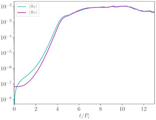
The time evolution of the average values of the toroidal |$B_T=\sqrt{B^\phi B_\phi }$| and poloidal |$B_P=\sqrt{B^2 - B_T^2}$| components of the magnetic field.
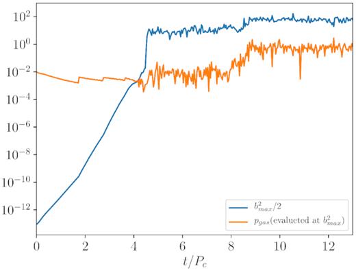
Time evolution of |$p_\mathrm{mag}=\frac{1}{2}b^2$| and pgas ≡ p, both evaluated where pmag takes its maximum value.
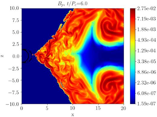
The three phases are more clearly apparent in Fig. 3, where spatial maps of the (poloidal) magnetic field are presented (in logarithmic scale) at three different times. In the upper panel we are clearly still in the kinematic, linear phase of the dynamo. The magnetic field does not affect the disc shape, magnetic islands corresponding to the linear dynamo modes migrate towards the outer edge of the disc while growing in amplitude. In the middle panel, the disc starts to be affected by the presence of the growing field and dynamo waves are dragged towards the black hole by the accretion. The accretion process is most probably triggered by MRI (see the discussion below), that also drives turbulent motions. In this dynamic regime, magnetic structures tend to form low-pressure vortices that drag matter away (bottom panel), that for high values of the magnetic field can even evacuate the plasma locally (and safety floor density values can be required numerically, in order to limit this effect). The dynamo modes are barely visible during the phase of the secondary growth (third panel), and they seem to be localized only at the external boundary of the disc, where density and the dynamo term ξ are lower (this point will be addressed in the next section).
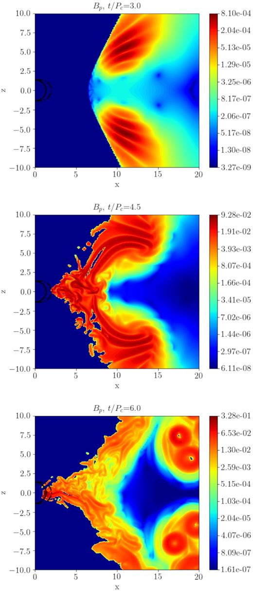
Colour maps of the poloidal magnetic field BP in logarithmic scale, for three different times t/Pc. Black lines near the origin are the contours of the black hole’s ergosphere (dashed line) and horizon rh (solid line).
4.1 Dependence on the α-dynamo number and on the quenching effect
We now investigate the dependence of the results on the α-dynamo number Cξ and on the employment of an explicit quenching effect (see below). The list of runs with the corresponding parameters is reported in Table 2. In particular, Run2 and Run3 are characterized by increasing values of ξ and Cξ with respect to our reference Run1 values, whereas Run4 and Run5 by decreasing values of the same parameters. Fig. 4 shows the dependence of the exponential growth rates of the kinematic (γ1) and dynamic (γ2) phases, respectively, with the dynamo number Cξ. Growth rates are measured for both the poloidal field component (blue triangles) and for the toroidal one (blue circles), values also reported in Table 2. The red symbols indicate the corresponding quantities for simulations where quenching is active (labelled with a ‘q’ in the table of runs).
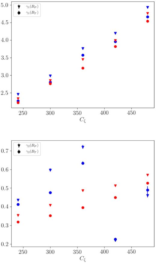
Dependence of growth rates γ1 and γ2 on the dynamo number Cξ. Triangles (circles) for the poloidal (toroidal) field components, blue (red) colour for runs without (with) quenching.
We observe that the rates γ1 corresponding to the kinematic phase follow a linear trend, as expected, whereas the rates γ2, corresponding to the phase where accretion affects the dynamo modes, show an unexpected drop at high values of ξ (blue symbols). This may be due to the rapid growth of the magnetic field, leading to values able to modify the fluid equilibrium itself. This seems to prevent, or at least to lower, a subsequent amplification, as if a saturated state has been reached.
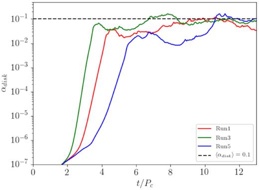
The quantity αdisc defined in equation (42) as a function of time, for three runs with different dynamo number Cξ.
The five runs have been repeated with identical parameters and the addition of the quenching effect, labelled as Run1q–Run5q in Table 2. As expected, the dynamo growth rates are basically unchanged in the quasi-kinematic phase. However, now the rates γ2 appear to grow linearly with Cξ, exactly as rates γ1, even in the phase where turbulence and accretion are present (see the red symbols in Fig. 4, for both γ1 and γ2). Notice that below Cξ = 400 the γ2 values are lower than the corresponding cases without quenching, as expected, but higher above that value, where however the blue data looked pathological since no regular trend was followed. Four additional runs with Cξ increasing from ≃750 up to ≃1800 have also been performed, again in presence of the quenching term. The linear trend for γ2 is less evident than what shown in Fig. 4, though we find a final value γ2 ≃ 1.5, that is more or less what one would expect from a linear extrapolation.
These results show that the dynamo appears to be the main mechanism for amplifying magnetic fields even during the phase in which the disc starts to lose mass, which is accreting on to the black hole. Furthermore, when quenching is activated, since a lower magnetic field is present, the formation of vortices evacuating the plasma is inhibited and the dynamo structures evolve more smoothly even in a turbulent environment, as clearly shown in Fig. 6.
Map of the poloidal field (in logarithmic scale) for t = 6Pc (Run1q, with quenching), to be compared with the third panel of Fig. 3 (Run1, without quenching).
In order to better clarify why the secondary growth rate γ2 is lower than the corresponding γ1, we plot in Fig. 7 the time series of the spatial averages of the Cξ dynamo number. We clearly see that, when the accretion begins and the first saturation phase starts, the quantity decreases for all runs without the quenching term and for Run3q as well. This is due to the fact that during accretion the density can be modified substantially, and |$\langle$|Cξ|$\rangle$| as well, and this effect is stronger for higher magnetization levels. When the quenching term is present both magnetization and turbulence are generally lower, the presence of the low-density vortices is avoided, and the overall dynamics is certainly more regular. In any case, especially for runs with quenching, the lower values of γ2 cannot be attributed to correspondingly smaller values of |$\langle$|Cξ|$\rangle$|, while migration of the plasma near the border of the disc, where Cξ is reduced, appears to be more important. In addition, when the density is low, the other dynamo term, |$C_\Omega$|, gets larger values, and for a constant Cξ the overall growth rates are expected to be reduced (see table 1 in Bugli et al. 2014).
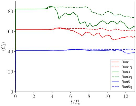
Time series of the dynamo number Cξ averaged over the whole disc.
A very interesting result is that the value of Cξ and the presence of quenching do not affect too much the value of the quantities in the final saturation stage, as can be seen in Fig. 8, where the growth of the average strength of the magnetic field is plotted for our six reference runs. The initial kinematic growth and also the first saturation phase clearly depend on Cξ, as the fastest growing mode occurs at a wavenumber ∼ξ/η (Brandenburg & Subramanian 2005), with smaller scales triggered by MRI leading to a turbulent cascade towards the dissipative scales. However, the second and final saturation phase looks approximately independent on the Cξ value and on the presence of quenching (all curves tend to the same value of |$\langle$|B|$\rangle$| within a factor of ≃3), hence we deem that the accretion dynamics and the reached equipartition with the fluid component play a major role at this final stage (see the similar behaviour of αdisc).
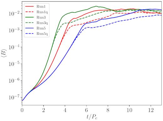
Time evolution of the averaged intensity of the magnetic field, for three runs without and with quenching.
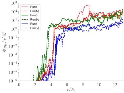
Time evolution of the magnetic flux ΦBH penetrating the horizon, divided by the accretion rate, for the same six runs as in Fig. 8.
4.2 On the magnetorotational instability
In the non-linear regime it is interesting to investigate whether MRI is capable of affecting the dynamo action or, more generally, of changing substantially the structure of the magnetic field.
Fig. 10 shows the time evolution of the factor Qθ, averaged over the whole disc, in the case of Run1. Apparently the MRI instability could be resolved during the dynamical phase and therefore, if present, it would be expected to play a role in the growth of the magnetic field, competing with the ongoing dynamo process.
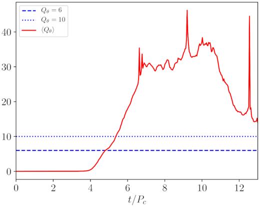
Time dependence of the averaged MRI quality factor Qθ, for Run1 parameters. The two horizontal lines are the thresholds for resolving the linear (dashed line) and non-linear (dotted line) phases.
To investigate this aspect we have re-executed Run1 twice, the first time by setting ξ = 0 for t/Pc > 4.5, at the end of the first linear stage, and the second one for t/Pc > 8.0, just before the final saturation after the second linear phase. As we can see in Fig. 11, the magnetic field components immediately start to decrease after the dynamo has been switched off, in both cases. Notice that the poloidal component is the one suffering the fastest decrease, the toroidal one is probably still supported by a residual amplification due to rotation (a purely Ω effect).
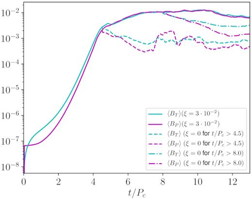
Growth of the magnetic field components for Run1 and for two additional runs with the same parameters but switching off the dynamo (ξ = 0) for t/Pc > 4.5 (dashed lines) and for t/Pc > 8.0 (dot–dashed lines).
This result means that the dynamo action is the main driver for magnetic field enhancement in all phases, whereas MRI, which is surely present and resolved numerically in our simulations, seems to be responsible mainly for triggering turbulence and driving the accretion. Amplification of magnetic fields by MRI is instead less strong than the one due to the mean-field dynamo (we recall that our simulations are 2D axisymmetric), and its effect is only visible in the final saturation stage, where a faster decrease due to dissipation is inhibited. We conclude by saying that the adopted resistivity value of η = 10−3 is still above the level of numerical dissipation, which is estimated to be η ∼ 10−4 for the resolution employed.
4.3 Comparison with Sgr A* radio emission
Our GRMHD models based on the dynamo action will be used here to infer the synthetic emission by the magnetized plasma of the accreting matter and to compare it with observational data. The most straightforward targets are obviously the two sources observed by EHT, Sgr A* and M87*, i.e. the cores containing the supermassive black holes of our Galactic Centre and of the elliptical galaxy M87. In the latter case, the very first image of the emission from the regions around a black hole’s event horizon has been recently taken (EHT Collaboration 2019a), whereas at the moment work is in progress to reduce data in the case of Sgr A*.
Since our simulations are more focused on the plasma dynamics occurring inside the disc, with the magnetic field growing from initial seed values, we choose here to compare our model with Sgr A* data, as in the case of M87* a substantial fraction of the emission is known to come from the polar jet. The structure of Sgr A* is rather uncertain because the source is hidden by optically thick interstellar medium that surrounds it. For this reason models with or without a jet have been built over the years to infer its emission properties (Mościbrodzka et al. 2009, 2014; Mościbrodzka & Falcke 2013).
The radio emission in the mm band of the Sgr A* spectrum can be modelled by the radiation produced by thermal synchrotron-emitting relativistic electrons in an ADAF/RIAF (Advection-Dominated Accretion Flow and Radiatively Inefficient Accretion Flow) model. According to the theory, most of the energy is stored in the thick pressure-supported disc and advected inwards with high speed and efficiency. The large scale height and accretion velocity makes the density low, the gas cooling time long compared to advection times (the temperature of proton remains high, Tp ∼ 1011−1012 K), and the plasma is optically thin (Narayan, Yi & Mahadevan 1995; Narayan & McClintock 2008).
In the following, we show that our model (we choose Run1 and Run1q parameters) can predict that the initial magnetic field (∼10−4 G) is amplified by the mean-field dynamo up to a level able to explain the observed flux in the millimetric wavelengths. The three free parameters left, namely ν, Rhigh, and n0, are chosen as follows: ν is set to 230 GHz, the same used for M87*, Rhigh is fixed to 20, a reasonable value in the disc and n0 is chosen as the value that best reproduces the observed flux of 2.64 ± 0.14 Jy at 230 GHz (Mościbrodzka & Falcke 2013; Mościbrodzka et al. 2014; EHT Collaboration 2019a). Let us look at Fig. 12. The predicted synthetic flux follows the average magnetic field trend, increasing until it reaches a quasi-stationary value. We perform a time average in the range t/Pc = [7−13], obtaining a flux of 2.59 Jy consistent with the observations when assuming n0 = 6.5 × 107 cm−3 for Run1 and n0 = 5.5 × 107 cm−3 for Run1q.
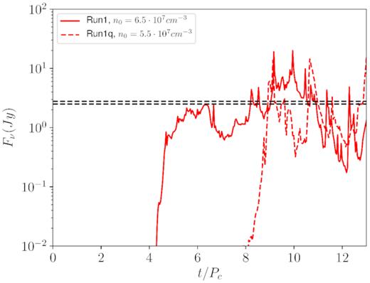
Time evolution of the synthetic flux Fν computed on top of Run1 (solid line), and of Run1q (dashed line). The horizontal dashed lines represent the observed value at for the reference frequency ν = 230 GHz.
In Fig. 13 (upper panel), we show the time evolution of the maximum value of the magnetic field in the disc, reaching Bmax ≃ 3−4 kG at the saturation of the dynamo process. At the same time, the average electron temperature reaches |$\langle$|Te|$\rangle$| just below 1011 K (lower panel). Overall these quantities result in agreement with the values obtained in the simulations of Mościbrodzka et al. (2009) and Mościbrodzka & Falcke (2013).
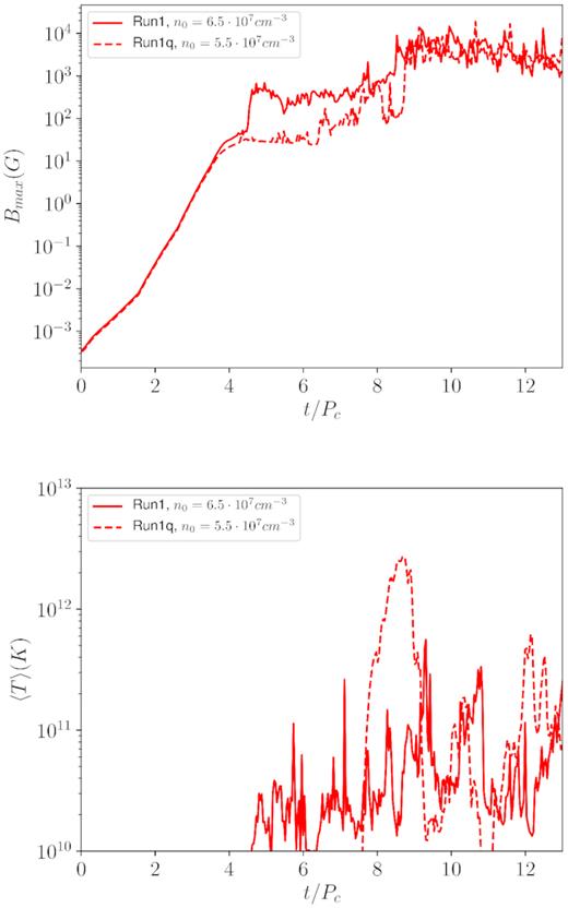
Time evolution of the maximum value of the magnetic field strength (upper panel) and of the average electron temperature (lower panel) for Run1 (solid line) and of Run1q (dashed line).
5 SUMMARY AND CONCLUSIONS
In this paper, we have investigated, for the first time by means of non-ideal axisymmetric GRMHD simulations, the mean-field dynamo process operating in thick accretion discs around black holes, in the fully non-linear regime. This work can be seen as a follow-up of our previous analysis in the purely kinematical regime (Bugli et al. 2014).
Similar GRMHD simulations have been recently employed to model the dynamics and emission of the central core of the galaxy M87 (EHT Collaboration 2019b), comparing with observational data including the very first image of the shadow of a black hole’s event horizon (EHT Collaboration 2019a). Contrary to the standard numerical initial set-up, where a subdominant but non-negligible magnetic field (pmag/p ∼ 10−2) is present in the disc right from the start (e.g. Porth & EHT Collaboration 2019), here we initialize the simulation with an extremely small magnetic field (pmag/p ∼ 10−9), which is later self-consistently amplified during the evolution by the α−Ω dynamo process.
A linear kinematic exponential growth, followed by an other one with reduced rate when accretion becomes important, is observed for a variety of dynamo parameters. Both rates increase linearly with the dynamo parameter at least for the limited range explored here. The dynamo is clearly the main driver, with the second, reduced stage due to the fact that due to accretion the density in the disc is modified and the non-dimensional dynamo number Cξ reduces in time, especially for runs with a stronger dynamo. At later times the accretion process and the stronger field are capable of affecting the overall structure of the disc itself and the growth of the magnetic field ceases, reaching a saturation phase where the magnetic field is approximately constant in time. The presence of an explicit quenching term in the α-dynamo shortens the linear phase but seems not to affect the final saturation stage, occurring roughly for similar values of the magnetic field strength (within a factor of three). The quenching also helps in avoiding the formation of a few pathological structures with highly magnetized vortices evacuating the plasma in the outer disc regions, and the overall dynamics is more regular.
In spite of the widely recognized importance of MRI for global simulation of discs around black holes (e.g. Bugli et al. 2018, and references therein), and in spite of our simulations having the sufficient spatial accuracy to resolve such instability (the MRI quality factor Q exceeds 10 after a few rotational periods), this does not seem to play a major role here, if not as an initial trigger for the turbulent cascade and accretion on to the black hole. We have tested this hypothesis by switching off the dynamo term at the end of each growth phase (in different runs with otherwise the same parameters): the field starts to decrease immediately, and MRI seems to be just capable of balancing dissipation at small scales, reaching a steady (turbulent) state at late times.
By assuming the approximation of an optically thin plasma, as expected for Sgr A*, the accreting supermassive black hole of our Galaxy, we have computed on top of our simulations the expected emission, at millimetre wavelengths, for such source. A two-temperature plasma and all the recipes commonly employed for ADAF/RIAF systems have been used, obtaining very reasonable results, compared to previous works (Mościbrodzka et al. 2009, 2014). This confirms that the dynamo action, believed to occur in these systems due to small-scale turbulence, is capable of amplifying the magnetic fields, in a self-consistent way, up to the values required to reproduce the observations.
All simulations have been performed with our echo code (Del Zanna et al. 2007), which has recently successfully participated to a code comparison project by the EHT collaboration (Porth & EHT Collaboration 2019), in the upgraded version to include non-ideal resistive and dynamo effects in the Ohm’s law (Bucciantini & Del Zanna 2013; Del Zanna & Bucciantini 2018). From a computational point of view, we have here improved the implicit version of the conservative-to-primitive inversion step, by providing for the first time the analytical Jacobian matrix needed in the 3D Newton–Raphson scheme. A similar approach has been recently employed for purely resistive schemes (Mignone et al. 2019; Ripperda et al. 2019).
To conclude, we believe that non-ideal resistive-dynamo models of accreting discs around black holes represent a necessary upgrade to the existing ideal ones. However, for a detailed comparison against the revolutionary images by the EHT collaboration, fully 3D simulations and ray-tracing techniques in curved space–times are certainly required.
ACKNOWLEDGEMENTS
The authors are grateful to the anonymous referee for very helpful suggestions. Numerical calculations have been made possible through a CINECA-ISCRA project and a CINECA-INFN agreement, providing access to resources on MARCONI at CINECA. We acknowledge financial support from the ‘Accordo Attuativo ASI-INAF no. 2017-14-H.0 Progetto: on the escape of cosmic rays and their impact on the background plasma’ and from the INFN Teongrav collaboration. MB acknowledges support from the European Research Council (ERC starting grant no. 7153 68 – MagBURST).
Footnotes
REFERENCES
, in
APPENDIX A: THE COEFFICIENTS FOR THE ELECTRIC FIELD AND FOR ITS JACOBIAN
In the present Appendix, we show how equation (16) has been derived and we provide the expressions for the required coefficients of Γ and of their derivatives, to be used in equation (22). Since we are working with spatial vectors alone, involving the 3D metric tensor γij (not diagonal in Kerr–Schild coordinates), we use here for simplicity the standard vector notation, for which |$\boldsymbol {v}$| is employed rather than vi.
