


ABSTRACT
The applicability of a linearized perturbed FLRW metric to the late, lumpy universe has been subject to debate. We consider in an elementary way the Newtonian limit of the Einstein equations with this ansatz for the case of structure formation in late-time cosmology, on small and large scales, and argue that linearizing the Einstein tensor produces only a small error down to arbitrarily small, decoupled scales (e.g. Solar system scales). On subhorizon patches, the metric scale factor becomes a coordinate choice equivalent to choosing the spatial curvature, and not a sign that the FLRW metric cannot perturbatively accommodate very different local physical expansion rates of matter; we distinguish these concepts, and show that they merge on large scales for the Newtonian limit to be globally valid. Furthermore, on subhorizon scales, a perturbed FLRW metric ansatz does not already imply assumptions on isotropy, and effects beyond an FLRW background, including those potentially caused by non-linearities of general relativity (GR), may be encoded into non-trivial boundary conditions. The corresponding cosmologies have already been developed in a Newtonian setting by Heckmann and Schücking and none of these boundary conditions can explain the accelerated expansion of the universe. Our analysis of the field equations is confirmed on the level of solutions by an example of pedagogical value, comparing a collapsing top-hat overdensity (embedded into a cosmological background) treated in such perturbative manner to the corresponding exact solution of GR, where we find good agreement even in the regimes of strong density contrast.
1 INTRODUCTION
The late universe, a slice of which is visible to galaxy surveys on our past light-cone, is very clumpy. This is in stark contrast to the earlier universe: the observed fluctuations in the cosmic microwave background (CMB) are small (Aghanim et al. 2018), allowing for a precise interpretation of their properties based on linearized, relativistic cosmological perturbation theory that is well established (Durrer 2008). However, gravitational collapse has transformed the smooth state into one that cannot be evolved anymore by effective fluid equations (Baumann et al. 2012) without removing short scales of comoving size of a couple of Mpc, and certainly not by linear equations.
The conceptually simple, but technically challenging, non-linear Newtonian Vlasov–Poisson system (Peebles 1980) describes the gravitational amplification of dark matter structures including smaller scales and large density contrasts. Newtonian N-body simulations have tackled the challenging prediction of the structures’ morphology, solving this system by sampling its characteristic curves. There is no doubt that Newtonian theory is capturing the gravitational physics of finite astrophysical systems such as galaxies or clusters of galaxies, where gravity is weak. We similarly expect Newtonian physics to approximate sufficiently localized cosmological patches when fields are weak and matter is moving slowly (Peebles 1980; Kaiser 2017), including the non-linear evolution of matter beyond linear cosmological perturbation theory. However, in cosmology, we are interested in global solutions, and the validity and generality of a Newtonian approximation is not immediately clear when going to large scales.
The Newtonian limit of general relativity (GR) may therefore be studied carefully in the context of large-scale structure in cosmology (Peebles 1980; Holz & Wald 1998; Green & Wald 2012). The limit involves linearizing the Einstein tensor for weak fields around a background. The choice of this global background solution is non-trivial. Instead, a local approach aims to avoid this step and it has been shown how gluing together patches close to the Minkowski space–time in a bottom-up construction yields cosmological solutions of GR (Sanghai & Clifton 2015), that is, the background emerges and can be compared to the predictions of Newtonian cosmology. Therefore, a local approach can help clarifying the generality of the Newtonian limit in cosmology, which is crucial when building simple models for reaching robust conclusions about our universe comparing to observations. For example, the report in Rácz et al. (2017) of large relativistic acceleration effects beyond Newtonian cosmology without the need for dark energy produced in simulations with a modified N-body code has recently received a critical reply Kaiser (2017) in which the backreaction proposal (see e.g. Buchert & Räsänen 2012) was discussed assuming a Newtonian setting. However, any significant differences of Newtonian and GR cosmological dynamics claimed to invalidate this reply (Buchert 2017) must be related to assumptions made when taking the Newtonian limit of GR, and the discussion can be supplemented by this step. Beyond foundational questions in GR, a Newtonian limit is still the foundation for obtaining the leading-order corrections to structure formation from covariantly formulated modified gravity theories, by using N-body simulations that have been modified accordingly. Furthermore, the Newtonian limit is the relevant approach for properly addressing cosmological effects on cosmologically very small systems, like the Solar system (or even an atom Bonnor 1999; Price & Romano 2012), both for GR (Dicke & Peebles 1964; Bonnor 1996; Cooperstock, Faraoni & Vollick 1998; Carrera & Giulini 2010; Nandra, Lasenby & Hobson 2012b) and modified gravity. Constraints on the time evolution of the Newton constant obtained in the Solar system (Pitjeva & Pitjev 2013; Hofmann & Müller 2018; Fienga et al. 2015) and therefore on modified gravity are already below one per cent of the Hubble rate, and are becoming stronger with observation time with dramatic implications for some models (Belgacem et al. 2019).
In this paper, we are concerned with a correct leading-order treatment of non-linear structures in late-time cosmology. This is complemented by recent works on more general expansions of GR for a highly accurate description of our universe (Adamek et al. 2013, 2016; Fidler et al. 2017; Milillo et al. 2015; Goldberg, Clifton & Malik 2017).
On the other hand, it is usually stated that the metric scale factor in equation (1) should be the one of a best-fitting background universe. When perturbations in equation (1) are neglected ‘on average’, and if the background energy density is assumed to be the Newtonian spatial average of the physical density, the metric scale factor obeys the same Friedmann equation of the homogeneous ball of matter in Newtonian theory. Since the Einstein equations are non-linear, a background scale factor based on Newtonian averaging may seem as a shortcut lacking rigorous justification (Kolb, Marra & Matarrese 2010; Wiltshire 2011). Furthermore, if the ‘correct’ scale factor must be chosen in equation (1), corresponding to some average Hubble flow, the intuition may be that situations where matter locally moves with very different expansion rates (e.g. after turnaround) cannot be small perturbations as assumed in equation (1, Räsänen 2010). However, it has also been shown that Lemaître–Tolman–Bondi (LTB) solutions with locally different expansion rates of matter can be mapped to perturbed FLRW if the inhomogeneities are confined to subhorizon scale (Van Acoleyen 2008; Yamamoto et al. 2016). This supports the validity of the ansatz (1), but clearly questions the physical relevance of the scale factor in the metric on small scales, similarly to its introduction as a coordinate choice in Newtonian cosmology.
We therefore studied GR cosmology using a perturbed FLRW metric and guided by the observed properties of dark matter at low redshifts, emphasizing a local approach. To leading order, we recovered the validity of a linearization of the Einstein tensor and obtained a consistent Newtonian limit. These results can be illustrated by an explicit example: the simplest, most extreme (and therefore most interesting) space–time describing a collapsing object within the expanding universe is arguably that of a top-hat profile – a homogeneous core surrounded by an empty shell – embedded into a matter-dominated universe. We confirmed that the perturbed FLRW metric is able to describe this situation; it can thus simultaneously accommodate structures with very different expansion rates. As a key step in the argument, we derived explicit coordinate transformations that can change the scale factor non-perturbatively from being solution of one Friedmann equation to a solution of another Friedmann equation, while keeping the potentials perturbative. We also found that on subhorizon scales and allowing for Ψ ≠ Φ the scale factor in the metric (1) is arbitrary, whereas it emerges on large scales for a correct description of the geometry, where it eventually must correspond to the physical motion of matter. We checked this gauge freedom of a(t) by repeating the analysis of the top-hat example using the perturbed FLRW metric with another choice of scale factor.
Due to the local and constructive approach, the calculations are general enough to have implications for the backreaction proposal. On small scales, where the scale factor of the perturbed FLRW metric is arbitrary, the effect of GR solutions is constrained free of the assumption that the global background is an FLRW space–time. Since local cosmological tests take place in this regime, dark energy can be probed disentangled from potential relativistic effects on the dynamics.
The paper is structured as follows. Section 2 reviews the Newtonian limit for late-time cosmology and derives the starting point of Newtonian cosmology from GR in the general setting of arbitrary scale factor. Section 3 then introduces the top-hat space–time in detail in Section 3.1, tests the FLRW metric in the standard case in Section 3.2, and subsequently confirms the result of Section 2, for Ψ ≠ Φ with a non-standard choice of scale factor in Section 3.3. Before we conclude in Section 5 we discuss in Section 4 in some detail the large-scale limit (Section 4.1), the meaning of cosmic expansion for local systems (Section 4.2), the transition from covariance to inertial frames (Section 4.3), and the assumptions that have been made with the FLRW metric and the implications for the backreaction proposal (Section 4.4).
2 NEWTONIAN LIMIT
2.1 Weak-field, slow-motion expansion scheme
We can develop an expansion scheme based on a non-relativistic velocity v ≪ 1 and anticipating that the potentials Ψ and Φ, in this section collectively denoted as ϕ, behave similarly to Newtonian potentials and obey a Poisson equation sourced dominantly by the matter density fluctuations corresponding to the observed morphology. For simplicity and because we are considering the late universe we shall set a ≈ 1 in the following explanation; comoving spatial coordinates x can be thought of as physical.
We assume further that the vector perturbation |$\boldsymbol {B}$| is of order |$\mathcal {O}(v^3)$| and behaves similarly to the potentials under derivatives. For further discussion of the scheme and the literature, it is more practical to see the equations first.
2.2 Field equations
Reiterating on the comment around equation (8) above, on very small and fast scales, the result (18) should be thought of as Ψ − Φ ∼ 0 (to lowest order). The right-hand side is a cosmological term ∝ k(t)r2 that automatically loses significance on small scales. In fact, near r = 0 the Laplacian of Ψ − Φ may actually be dominated by space-dependent post-Newtonian terms. These new terms arise from solving equations to next order containing now both terms like |$\ddot{\phi }$| in equation (12) as well as quadratic terms like ϕ∂2ϕ in (10) (which are of similar size). However, since ∂2ϕ still dominates ϕ∂2ϕ, the post-Newtonian terms are subleading and the statement Ψ = Φ (up to a constant) is now correct to leading order if the cosmological term ∝ k(t)r2 is even smaller. This is for example true when restricting to Solar system scale, where we know how small the post-Newtonian corrections are. Therefore, while one could drop the cosmological term in e.g. equation (12) on such scales to emphasize it is not the largest subleading correction, it is not necessary when the goal is only a valid leading-order treatment. As written, the equation holds also on cosmological scales.
On the other hand, studying the full linearized Einstein equations including terms like |$\ddot{\phi }$| in equation (12) while setting Ψ = Φ, which removes spatial derivatives from equation (12, and which is obtained from excluding terms like ϕ∂2ϕ and gauging α(t) = 0) leads to unphysical results for large density contrasts (Räsänen 2010) and is incorrect given the physical setup because |$\ddot{\phi } \sim \phi \partial ^2 \phi$|. Blind application of the standard cosmological perturbation theory treatment developed for small density contrasts, when a perturbative expansion in powers of the potential is well behaved, does break down for large-scale structure. This does not imply that proper leading-order physics cannot be obtained from a linearized treatment like ours. Instead of being forced to include quadratic terms or higher, the easier solution is to drop certain linear terms by changing to an expansion scheme that tracks powers of v.
The expansion scheme discussed here can also effectively be obtained in Fourier space of linear perturbation theory in a subhorizon limit, which we see a posteriori. By taking the leading terms when k → ∞ and before any manipulations that use δ ≪ 1 (and by selecting a Newtonian source) the expansion discussed here is recovered, but only for the special gauge of α(t) = 0. In the Fourier space approach polynomial growth in real space is easily missed. Typically, one introduces background equations to define sources of vanishing volume average to be able to divide by k2.
2.3 Friedmann equations as a gauge choice
From equation (18), any other gauge choice implies the set-in of a quadratic divergence for the difference of the two potentials, and therefore for at least one them in the metric. The Friedmann gauge choice is thus relevant when constructing a global perturbed FLRW solution, to be discussed below in Section 4.1.
If we are interested in a patch of the universe of size much smaller than the Hubble scale, a growth of the potentials |$\sim H_0^2 r^2$| is of no concern. In this case a(t) is allowed to depart from the Friedmann solution by |$\mathcal {O}(1)$|. Instead of satisfying equation (22), a(t) may satisfy (17) for α(t) ≠ 0 chosen with |$\alpha (t) \sim H_0^2$|. This preserves the condition for small peculiar velocities on subhorizon scales (14). The scale factor is therefore directly related to an arbitrary gauge freedom in the subhorizon limit.
As discussed above, Ψ − Φ also contains small non-linear terms and time derivatives of the potentials, which dominate the quadratic difference on sufficiently small scales, so Ψ ≃ Φ restricted to very small scales does not imply Friedmannian scale factor evolution. Instead, the scale factor remains unconstrained in its cosmological evolution. This is expected, because the choice of scale factor should become completely irrelevant on these local scales. In particular it may still be chosen to obey a gauge like equation (23) for a treatment unified with larger scales.
2.4 Motion of matter
We now show that we indeed obtain the proper Newtonian limit independent of the choice of scale factor.
3 EMBEDDED TOP-HAT COLLAPSE
To test the gauge freedom of the scale factor and the applicability of the perturbed FLRW metric in situations of strong inhomogeneity, we consider a spherically symmetric example with Λ = 0 for simplicity. For radial motion, T0i is irrotational and we can set |$\boldsymbol {B}=0$| in the following. In particular, we consider the collapse of a pressureless dust top-hat (core region), leaving behind a vacuum shell, embedded into the matter cosmos.
To understand our example, it is useful to be aware of the Einstein–Straus solution (Einstein & Straus 1945, 1946; Carrera & Giulini 2010). It serves as an even simpler toy model of a collapsed structure in the expanding universe and can be thought of as the end result of a spherical collapse in the following sense: it represents what is obtained from a matter-dominated universe by compressing the dust contained within a ball of arbitrary size into a black hole. The dust outside of the vacuum bubble created in this way continues its usual expansion not only in Newtonian gravity but also, exactly, in GR. The vacuum bubble is therefore bounded by a shell of fixed comoving radial coordinate and expanding in physical coordinates (for standard comoving coordinates adjusted to the initial Hubble flow). An observer entering the bubble from the outside trying to remain at fixed comoving or physical coordinates needs to compensate a gravitational pull towards the centre that is increasing with decreasing distance to the black hole (starting at zero for the comoving case) and ultimately diverging at the Schwarzschild horizon, but the crossover into the bubble is smooth. An explicit solution in a single coordinate system is rather unwieldy in terms of formulae (Schücking 1954; Laarakkers & Poisson 2001; Balbinot, Bergamini & Comastri 1988), considerably more so than the solution McVittie found by direct integration of the Einstein equations (McVittie 1933; Nandra, Lasenby & Hobson 2012a) with a similar goal of describing a point mass embedded in an expanding universe, but the physical picture is simpler for the Einstein–Straus solution.
Instead of imposing a central black hole, we will be concerned with the previous weak-field stage of the collapse, for which the black hole is smoothed to a collapsing top-hat core similar to the Oppenheimer–Snyder model (Oppenheimer & Snyder 1939). The Oppenheimer–Snyder model is in some sense the most extreme yet simple case of collapse. The exact solution of a top-hat undergoing turnaround and collapse is a portion of the closed FLRW space–time (Misner et al. 2017).4 The combined Einstein–Straus–Oppenheimer–Snyder collapse has been discussed by other authors within GR (Nottale 1982; Dai, Pajer & Schmidt 2015; Kim, Lasenby & Hobson 2018). The density profile and its evolution is schematically illustrated in Fig. 1.
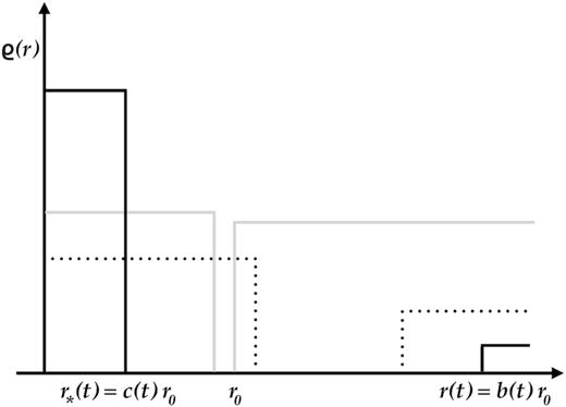
An example initial density profile is shown (grey) with a top-hat created by compressing the matter in a homogeneous universe within a spherical region. After some expansion (dotted), the top-hat turns around and collapses, whereas the outer universe continues to expand (black). The boundary of the top-hat is denoted as r*(t) and the outer boundary of the vacuum region as r(t). Their time evolution is parametrized by two scale factors c(t) and b(t), respectively.
We wish to model this space–time in the perturbed FLRW gauge, which will give a continuously differentiable but approximate solution in a single coordinate system by construction. Our strategy is to assess the quality of the approximation by comparing the result to the exact (closed FLRW, Schwarzschild, and flat FLRW) solutions separately for each of the three regions by finding appropriate coordinate transformations. This compliments the more complicated and less explicit result in Van Acoleyen (2008), which studies the validity of the perturbed FLRW solution by comparison to the exact LTB class of solutions, with the explicit top-hat collapse case that intuitively is the most challenging one for the perturbed FLRW metric.5
3.1 Newtonian top-hat collapse
We first use a physical radial coordinate r in which Newtonian theory holds in the usual way to describe some aspects of the collapse. Subsequently, we will work with two alternative choices of comoving coordinates.6 While it would be possible to stay entirely within the respective comoving coordinates for the calculations, this would double part of our work.
We now first explore the natural choice a(t) = b(t) and then the choice a(t) = c(t) for the metric scale factor. The latter choice can be valid if not only the top hat but the whole patch considered are small compared to the Hubble distance |$H_a^{-1}$| according to the discussion after equation (13).
3.2 Cosmological scale factor
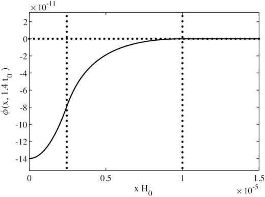
This plot shows the three matched pieces of the solution for ϕ in equations (47)–(49) for an overdensity obtained from first compressing the dust in a ball of radius |$r_0 = 10^{-5} H_0^{-1}$| to 0.4r0 (c(t0) = 0.4) and then letting it collapse until tf = 1.4t0. The vertical lines indicate the separation into core, vacuum, and outer cosmological region. The radial coordinate x is comoving with scale factor b(t). In the moment t = tf shown in the plot, b(tf) ≈ 1.66 (thus, if tf refers to today, t0 is at a redshift of 0.66). Initial velocities were aligned with the original Hubble flow; it follows that K = −2.34. The density contrast in the top-hat core, in the leftmost area of the plot, is δ = b3(tf)/c3(tf) − 1 ≈ 67, but the potential remains small everywhere.
3.2.1 External region x ≥ x0
Since ϕ = 0, the metric (44) is the FLRW metric for the EdS cosmos.
3.2.2 Vacuum region x*(t) < x < x0
In the following, we keep |$H_\mathrm{ b}^2 r^2$| and M/r as the smallest terms. The first one is very small compared to one if the vacuum region is very small compared to the Hubble distance, |$r_0 \ll H_\mathrm{ b}^{-1}$|, because x ≤ x0 and |$b = \mathcal {O}(1)$|; the second term is everywhere small under the weak-field assumption. We drop |$\sqrt{H_\mathrm{ b}^2 r^2} (M/r) = H_\mathrm{ b} M$| and smaller, and thus also Hbrϕ ≪ v2. In general, one cannot drop terms of order v3 (like |$\boldsymbol {B}$| itself) from the vector mode; however, only the transverse part of any vector mode enters in the continuity equation (26). We can therefore definitely ignore radial r − t off-diagonal terms of order v3 in the metric, corresponding to a longitudinal mode.
3.2.3 Interior region x ≤ x*(t)
3.3 Collapsing scale factor
where the formulae each again hold in the three regions now written as x ≤ r0, r0 < x < x0(t), and x ≥ x0(t), respectively. They are shown in Fig. 3. A comparison of the potentials Φ and ϕ from the previous section is shown in Fig. 4.
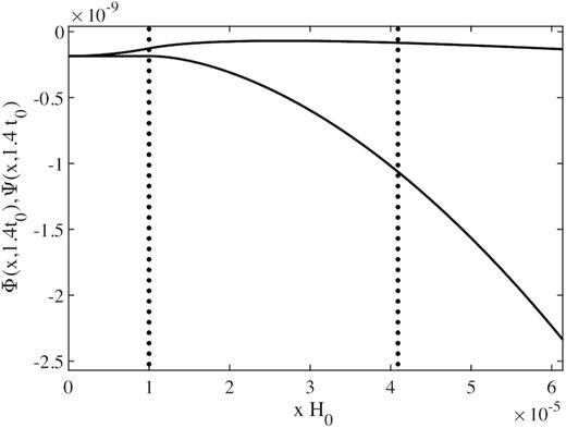
Shown are Φ (upper curve) and Ψ (lower curve) given by equations (83)–(86) for the same overdensity as in Fig. 2. Coordinates are now comoving with respect to scale factor c(t). Both potentials diverge quadratically on large scales since the scale factor does not correspond to the average motion there, but still remain small in a cosmological region of subhorizon size.

3.3.1 External region x ≥ x0(t)
It has to be noted that unlike before for the exterior region, this was shown only on subhorizon scales, because we have assumed smallness of the potentials which clearly both grow quadratically for this choice of scale factor. As discussed, on larger scales, the choice of a scale factor that leads to large peculiar velocities is not expected to be successful in the Newtonian limit.
3.3.2 Vacuum region r0 ≤ x ≤ x0(t)
3.3.3 Interior region x ≤ r0
This case would have been even simpler, namely not requiring a time transformation δt = 0 = ϵ, had we shifted the potentials by a (time-dependent) constant setting Ψ = 0 in the inside. A similar trick was used zeroing ϕ in the expanding scale factor case a(t) = b(t), exploited in Section 3.2.1. Here, we have illustrated that a non-zero constant related to γ(t) in equation (18) can be removed.
4 DISCUSSION
The coordinate transformations derived in the previous section validate the perturbed FLRW description for the embedded top-hat example for different gauge choices of the scale factor for a specific example. Here, we address some subtle points of the general Newtonian limit: the validity on large scales in Section 4.1, the Newtonian picture of structure formation in Section 4.2 and the relation of the linear part of the gauge freedom Ψ − Φ in equation (16) to the Newtonian cosmology developed by Heckmann and Schücking (1955, 1956) as well as implications for backreaction in the remaining two sections.
4.1 Emergence of Friedmann scale factor
On scales comparable to or larger than the Hubble scale, we have seen that the Newtonian limit can work only under a list of assumptions.
First, we need Ψ ≃ Φ and α(t) ≃ 0, so we may demand simply α(t) = 0 with the corresponding Friedmann solution (23) for a(t). Otherwise, if Ha departs by |$\mathcal {O}(H_0)$| from the Friedmann evolution, the difference of the potentials, and therefore at least one of them, approaches |$\mathcal {O}(1)$| at the Hubble scale, contradicting the assumption of small potentials used to derive the Newtonian field equations in Section 2.
Second, in Section 2, we have also requested that the physical Hubble flow is described by a(t) on large scales so that peculiar velocities can remain small far away from the coordinate center.
These two conditions are compatible, because the Friedmann equation for a(t) from the Einstein equations for Ψ = Φ and the Friedmann equation for the matter background that can be derived from the geodesic equation (38, done in Section 3.1 for the special case of vanishing cosmological constant) are in fact equivalent.
The smallness of the average of the source of the Poisson equation at early times becomes a statement about the flatness of the universe on large scales. If the average is not small at an early time, a curvature term may be introduced to balance the resulting divergence. The argument of the time-preservation of the absence of the divergence can be generalized to this case.
One is of course free to introduce another scale factor and coordinate system when solving the Newtonian equations after they have been obtained as described, and discussed in Kaiser (2017). However, only the Friedmann scale factor a(t) will be valid in the expression for the metric to describe the geometry of the space−time. In this sense, the a(t) given by equation (23) is emerging on large scales as a quantity that is useful for the description of the geometry.
4.2 Cosmic expansion force acting on local systems?
Many workers have investigated the influence of the global cosmology on the local dynamics. The classic results of Einstein & Straus (1945, 1946) are in accordance with the more general result (38) reported here that there is no local effect in a matter-dominated universe that cannot be explained in a simple manner by Newtonian gravity. In particular, Newton’s laws do not have to be ‘corrected’ for the ‘expansion of space’.
The cosmological constant does have an effect, investigated for example in Nandra et al. (2012b). More generally, any modification of the background evolution, be it homogeneous dark energy or infrared-modified gravity, replaces the cosmological constant by a term that is time dependent in general. This term can simply be understood as the Newtonian ‘weight’ of the dark energy component seen as a perfect fluid, when taking as given that pressure gravitates as predicted by GR. Note that N-body simulations are sensitive to modification of the background evolution because of this mechanism.12 All of this certainly has been known to some cosmologists for a long time (an early qualitative discussion is Dicke & Peebles 1964, see also Noerdlinger & Petrosian 1971), has been employed in studies of dynamics, e.g. in Lahav et al. (1991) and Falco et al. (2013), and forms the starting point of the success of Newtonian cosmology. An insightful discussion of the problem can be found in Dominguez & Gaite (2001), where the Newtonian shear effects are also investigated.
However, recent studies have sometimes come to more diffuse conclusions. These are often based on modelling the problem using exact solutions that contain a homogeneous component, like unperturbed FLRW for the the homogeneous universe (Cooperstock et al. 1998; Bonnor 1999; Price & Romano 2012), exact solutions describing a mass embedded into a universe with homogeneous density component like McVittie’s13 (Carrera & Giulini 2010; Nandra et al. 2012a), or others (Bonnor 1996), or they discuss several such models (Faraoni & Jacques 2007). On the other hand, the LTB solution does not contain a separate homogeneous component, and results directly agree with ours (Pavlidou, Tetradis & Tomaras 2014).
The homogeneous background components in the universe, more precisely a ball of cosmic fluids centred in the origin and extending up to a particle’s position, causes a force with magnitude proportional to |$\ddot{a} r / a$| according to Newton’s gravity, where a is the scale factor of the background cosmology obeying the Friedmann equations. (Indeed this is a valid way to derive the Friedmann equations, see Section 3.1 and Bertschinger 1995; Maggiore 2018.) The authors investigating local systems in cosmological backgrounds based on exact solutions often report such a force, but do not seem to appreciate that it can be understood in a simple Newtonian way. This is problematic when drawing conclusions about our realistic inhomogeneous universe. One must be aware of the local distribution of sources. For example, for vanishing cosmological constant, there is no cosmic force in the Solar system if and only if there is no dark matter in the Solar system, and conversely a force due to dark matter can be orders of magnitude larger than |$\ddot{a} r / a$| if the dark matter concentration is similarly higher. Regarding the cosmic effects on atoms, the importance of the nature of dark matter is then obvious.
In our view, it would be a particularly unnatural interpretation to attribute the effect instead to a long-range non-Newtonian force exerted from the ‘expansion of space’, which does not make sense in the Newtonian picture. Therefore, there is no need to argue against the validity of the physical picture given by the Einstein–Straus situation, even if it is not a realistic model neglecting the hierarchy of structures and demanding an exceedingly large vacuum bubble to compensate e.g. our sun (Carrera & Giulini 2010).
4.3 Newtonian inertial frames in cosmology
In an unperturbed Λ cold dark matter (ΛCDM) universe, the symmetry of homogeneity is incompatible with the Newtonian postulate of the existence of one particular class of inertial frames related by Galilean transformations. Two matter particles at two different locations feel a relative force and cannot both be at rest in, and define the origin of, an inertial frame of the same class. Clearly, there is no concept of a unique, global ‘absolute space’ for an infinite self-gravitating system. Even for a finite, expanding sphere there is no preferred inertial frame if observers at different locations are taken to be equivalently meaningful and ignorant of the boundary (McCrea 1955).
In this paper, we are faced with the general-relativistic emergence of the situation captured by this modification of Newtonian theory. On the one hand, for the starting point of the (unperturbed) FLRW metric, the transformation from one free-fall observer to another is a trivial translation generated by the obvious spatial Killing vectors. All comoving observers are geodesic and therefore simultaneously unaccelerated from a GR point of view. On the other hand, the Newtonian limit involves the transition to expanding physical coordinates which necessarily singles out the coordinate origin, seemingly breaking the symmetry. But the theory of GR and the FLRW ansatz on small scales with free perturbations naturally do not ‘know’ that our goal is to find Newton’s familiar equations written out in any inertial frame at all and certainly do not choose the origin for us.
And indeed, GR manages to preserve the symmetry of homogeneity due to gauge freedom.14 The function |$\boldsymbol {\beta }(t)$| is a degree of freedom arising when integrating Einstein’s equations that adds a linear term |$\boldsymbol {\beta }(t) \cdot \boldsymbol {x}$| to Ψ (and |$- 2 \boldsymbol {\beta }(t) \cdot \boldsymbol {x}$| to g00) according to equation (15). Again, in general, for |$\boldsymbol {\beta }(t)\ne 0$|, the negative gradient generates a global acceleration |$-\boldsymbol {\beta }(t)$| on a particle, as can be easily seen from the geodesic equation in the form of equation (32). In this case, one may boost to that proper frame which, as seen from the original one, undergoes the same acceleration. In Minkowski space, so on sufficiently small scales, such a boost precisely removes the linear term from g00 (Møller 1952), replacing it by the square |$(\boldsymbol {\beta }(t) \cdot \boldsymbol {x})^2$|. The effect of this remaining term in the geodesic equation must be neglected at leading order if we assume the acceleration happens on cosmic time-scales |$|\boldsymbol {\beta }| \sim H_0 v$|. While a detailed calculation of the boost for the perturbed FLRW metric on all scales goes beyond the scope of this discussion, we may conclude that the choice of |$\boldsymbol {\beta }(t)$| can be used on small scales and after taking the Newtonian limit to transform from one class of inertial frame to another, and in general, it allows for the description of the same physics from an accelerated frame. Therefore, setting |$\boldsymbol {\beta }(t) = 0$| (together with the assumptions in the next section) has the interpretation of selecting one of all the mutually accelerated classes of inertial frames compatible with homogeneity as our coordinate system.
It is worth pointing out a difference between the Newtonian and GR cosmology. Unlike in the Newtonian cosmology developed in Heckmann & Schücking (1956), the mathematically explicit homogeneity of the Newtonian cosmology obtained here from GR does not rely on the engineered boundary conditions (101), but emerges naturally from the field equations.
4.4 Boundary conditions and constraints on general-relativistic effects on the dynamics
We can further develop the discussion of possible effects from GR on the dynamics, under the assumption that gravitational waves can be neglected. Restricted to small scales, we will see that the assumption of a perturbed FLRW metric is weak enough and that we can understand the effects of cosmological solutions beyond an FLRW background despite the formal use of this metric. Specifically, we ask the questions if, first, it is possible within the approach under consideration that ignorance of the ‘right’ global background solution could lead to an order-unity effect on the matter motion on scales large enough to have cosmological applications, and, secondly, if this effect could look like cosmic acceleration. We will find that the answers are yes and no, respectively.
It is important to be mathematically slightly more precise in the rest of this section. To obtain a well-posed Dirichlet problem from the Poisson equation (9) or its Newtonian analogue (33), we must prescribe boundary conditions. We can define a boundary of a finite-sized (but large) patch of the universe under consideration and prescribe the potential on it. At first, we may ignore the gravitational effects caused by matter outside a spherical patch and set the source to zero there; note first that in the homogeneous case the Newtonian forces from each outer spherical shell cancel exactly. In the inhomogeneous Newtonian setting, the shearing caused by structures beyond ∼1 Mpc, which affects only non-spherical objects, has been estimated in Dominguez & Gaite (2001) to be negligibly small.
The effect of any different Green’s function (or boundary condition) is that of adding to the solution another homogeneous solution of the Poisson equation, i.e. a harmonic function. Among these are linear functions (planes). These have been fixed already in the previous section (e.g. to ensure that the centre of the spherical patch, where the potential gradient vanishes in the homogeneous setting, is the coordinate origin). The non-linear harmonic functions, on the other hand, have non-trivial gradients. For example, the small effect of the matter inhomogeneities outside the spherical patch could be reintroduced by a small deformation of the Green’s function. Furthermore, effects from the boundary at infinity17 in Newtonian cosmology or, as we will see below, from non-FLRW background solutions in GR are encoded in boundary conditions. Similarly, if the non-linear terms of GR were to conspire to give an effect at very large scales, this would have to appear as non-trivial boundary conditions of our patch.
In the complete theory of GR a choice of boundary conditions on a surface surrounding the region of interest is not required; providing initial data are enough.18 However, after taking the Newtonian limit, we have lost the information of the evolution of the boundaries. Thus, while the Green’s function is actually determined and cannot just be chosen to be equation (104), we are ignorant of it, also because we do not want to control the initial state in our approach on very large scales, preferring to restrict linearization to a subhorizon patch. Therefore, we simply consider the possibility of generic boundary conditions which can even be time-dependent. The only constraint we put on them is that they cause effects that are at most of order unity, that is, they cause additional forces comparable to the Newtonian forces, since even stronger effects are certainly not observed. Equivalently, we are allowed to add additional harmonic functions ϕh to the potential that have gradients comparable to those of the Newtonian potential obtained with equation (104).
It follows that these functions ϕh do not grow arbitrarily fast. Since we want |$| \nabla \phi _\mathrm{ h} | \lesssim H_0 v + H_0^2 r$| [again corresponding to the local forces and the Friedmann forces, respectively, equation (37)], they reach at most |$\mathcal {O}(1)$| at the horizon scale. Upon subtraction of an irrelevant constant, we therefore have ϕh ∼ v2 on subhorizon scales ≲ v/H0. This scale is already cosmological in the sense that the average matter density in a region of this size can be comparable to that of the cosmological constant, and the latter therefore effective in causing an accelerated Friedmann evolution of the patch. The approximations of Section 2 still hold. Furthermore, the choice of scale factor is irrelevant on this scale as discussed in Section 2.3 (cf. Section 4.1); in particular a = 1 is allowed, corresponding to an expansion around Minkowski space–time.19 It is clear that there is no additional input from the fact that the starting point was a perturbed FLRW metric. The situation is instead that locally a given metric, in fact general up to neglecting tensor modes and smallness of vector modes, satisfies Einstein’s equations for a given source to some required accuracy under the assumptions of Section 2, and uniqueness of the solution for given initial conditions implies that we are considering the right solution if the initial conditions are satisfied. Since we have encoded the non-trivial initial conditions in the scalar sector into the boundary conditions, which are still free, we are facing the general set of all relevant scalar sector solutions of GR for the local cosmological patch with a given dust source. In particular, as mentioned, there is no assumptions on isotropy at this point (within the limits of order-unity effects). As another example, locally, curvature of spatial slices can be realized perturbatively, as is clear from the example in Section 3, where the coordinate transformation between the curved FLRW metric for the collapsing core and the flat FLRW metric description was given. We conclude that on cosmological but subhorizon scales, the perturbed FLRW metric is a fully general ansatz for the relevant physics that does not imply a choice of background. On the other hand, we cannot trivially extend such a local treatment to horizon scales, because ϕh can become non-perturbative, just like Φ and Ψ − Φ for the wrong choice of metric scale factor. We have thus made the assumption of an FLRW background earlier when claiming that can Ψ and Φ remain small on large scales, making an implicit statement on their boundary conditions.
Despite the generality of the free boundary conditions, they cannot cause radial forces like the cosmic forces, including the accelerating one caused by a cosmological constant. To see this, note that the gradients of the harmonic functions ϕh are necessarily divergence-free. Therefore, by Gauss’ theorem, their flux through any closed surface must vanish, which is impossible for a radial force field. The gradients instead correspond to anisotropic (multipole) forces causing tidal shear. As mentioned above, the shear due to the inhomogeneity of the matter outside the patch is normally negligible in our universe (Dominguez & Gaite 2001). However, one can conceive cosmological models that are not based on an isotropic and homogeneous FLRW background. These effects can be modelled locally by non-linear harmonic functions ϕh since we have seen that this is the only remaining degree of freedom. It is interesting to note that these functions are in one-to-one correspondence with the different solutions of Heckmann–Schücking Newtonian cosmology selected by different boundary conditions (101) because those boundary conditions are precisely such that the solution to the Poisson equation is unique up to the addition of planes (Heckmann & Schücking 1956) and therefore they precisely fix the non-linear functions ϕh. Consequently, these general anisotropic Newtonian models, as well as their exact relativistic counterparts with non-trivial electric part of the Weyl tensor (Ellis 2009) in the Newtonian limit, admit a perturbed FLRW description by using some Green’s function different from equation (104) on subhorizon scales.
Conversely, if anisotropies are sufficiently constrained (which seems natural given the observed isotropy of the CMB), there cannot be large boundary conditions that break our perturbative treatment. The relevant solutions of GR are then restricted to be close to the FLRW type even on larger scales. We reserve a quantitative version of this argument for future work.
For a much more rigorous and more general discussion of backreaction, see Ishibashi & Wald (2005), and Green & Wald (2011, 2013, 2014).
5 SUMMARY AND CONCLUSION
We have justified and analysed the Newtonian limit of late-time GR cosmology with a perturbed FLRW ansatz including scalar and vector modes, following an approach in real space and implementing assumptions on the matter structures and motion based on observations. The vector mode of the metric can be used to absorb the transverse component of the time-space components of the energy-momentum tensor and does not enter elsewhere to leading order. The dynamics of CDM is Newtonian to leading order, which was discussed mostly assuming flatness and isotropy, although generalizations have been pointed out. The scale factor in the metric, or equivalently the spatial curvature at some instance, is a gauge choice on subhorizon scales and always drops out of the dynamical equations when they are formulated in a Newtonian frame. GR does not select the inertial frame; selecting it is another gauge choice. This can be understood as a consequence of the cosmological principle encoded in the FLRW geometry, and its implementation into Newtonian cosmology has previously been achieved in the Heckmann–Schücking formulation of the boundary conditions.
On large scales comparable or beyond the Hubble scale, given natural assumptions, the Newtonian limit works, but the scale factor appearing in the metric must be chosen to be close enough to the standard one compatible with the Friedmann equations with the right spatial curvature. In Fourier space, on horizon scales, one finds general-relativistic corrections which however correspond to Newtonian cosmology in changed variables (Green & Wald 2012). Since we work in real space to define accuracy, we are not concerned with these terms in this work.
Restricting to small vector perturbations and ignoring gravitational waves, GR does not allow for other dust cosmologies than those of Heckmann and Schücking (1956) on subhorizon scales. Therefore, comparing observations of structure on these scales to predictions derived with the perturbed FLRW metric are actually general if, in case it is of interest, anisotropic boundary conditions are allowed.
Consequently, measuring the cosmological dynamics on subhorizon scales can directly probe and disentangle the existence and nature of dark energy versus relativistic dynamical effects (encoded in boundary conditions). For example, one may study properties of galaxy clusters like the turnaround radius, see Hansen et al. (2019), and references therein. Less directly, one may restrict comparing clustering data to predictions based on the perturbed FLRW approach with various kinds of dark energy to subhorizon scales to restore model independence. On the other hand, supernova measurements of the expansion history have to extend to large distances of redshifts z ∼ 1 to make the effects of dark energy on the cosmological background dynamics visible, by going sufficiently far into the past on the light-cone instead of on particle trajectories, exceeding the subhorizon regime. On these larger scales, a more advanced treatment including GR cosmologies beyond FLRW backgrounds would be required to make the most of the data in particular if GR supports cosmologies that are both relevant for our universe and not simple large-scale extensions of the Heckmann–Schücking Newtonian cosmologies, such that new radial forces can emerge on large scales. However, this seems difficult to achieve without simultaneously violating observed isotropy already on smaller scales.
Furthermore, we fully agree with the Newtonian picture in Kaiser (2017) on the distinction of volume expansion and a scale factor that is a gauge freedom, and share the critique of the N-body simulation carried out in Rácz et al. (2017), where the two concepts were mixed, and the metric scale factor was locally adjusted to the expansion rate. We have shown that changing the metric scale factor in a patch must be accompanied by a change of metric curvature according to Einstein’s equations, and this in fact ensures that the Newtonian limit, which holds to leading order, is unchanged. Failing to do so simulates not relativistic physics beyond an FLRW background, but another theory than GR.
We conclude that the perturbed FLRW ansatz provides a consistent physical picture. It works as well as one could possibly hope for for the embedded top-hat model we have studied, for which the exact solution is known. From this analysis, there are no concerns for using the perturbed FLRW metric to simultaneously describe cosmology and much smaller scales like the Solar system.
The equations of motion for matter can be generalized e.g. to include frame dragging from the vector mode. In Castiblanco et al. (2019), the authors claim that the relativistic dynamical corrections beyond the Newtonian limit can have a very significant effect on the squeezed bispectrum due to the combination of different scales, at least when evaluated in perturbation theory. If confirmed by non-perturbative numerical studies, this would limit the success of Newtonian cosmology (amended with relativistic light propagation) in the perturbed FLRW metric (1) for late-time large scale structure.
ACKNOWLEDGEMENTS
I thank Michele Maggiore, Pierre Fleury, and Enis Belgacem for many crucial discussions and encouraging support and Pierre Fleury for a careful reading of the manuscript and insightful comments. Ruth Durrer, Steen Hansen, Nick Kaiser, David F. Mota, and Clément Stahl, as well as the anonymous referee, have also provided well-appreciated feedback on various aspects of this work. My work is supported by the Fonds National Suisse and the SwissMAP National Center of Competence in Research.
Footnotes
It should be noted at this point that seemingly circular reasoning like this is not problematic when solving differential equations as long as the final solution is self-consistent and satisfies all required boundary conditions under some assumptions ensuring uniqueness of the solution. (We also assume that an exact solution is obtainable continuously from minute deformations of the approximate result.) Instead of circular reasoning, this approach may be seen as an educated guess of a solution. There are however subtleties: besides not discussing tensor perturbations here, boundary conditions, required for uniqueness, will be addressed below. For now, we are still in the process of checking self-consistency.
It is also easy to miss these terms when working in Fourier space.
It appears that in this form the vector modes of FLRW were already discussed in Thomas, Bruni & Wands (2015).
The original interior Oppenheimer–Snyder solution (Oppenheimer & Snyder 1939) is actually equal to a patch of time-reversed flat EdS which does not allow for a turnaround.
A reader familiar with the LTB solutions may think that the embedded top-hat collapse should be a special case. Indeed, LTB solutions exactly describe more general inhomogeneous dust distributions with spherical symmetry. However, a single LTB metric is not able to cover the space–time considered with one set of coordinates. The gauge (gtt = −1, diagonal) is too constraining for each region so that one inherits the discontinuities from the discontinuous source.
To be clear, again the word ‘comoving’ refers only to the use of FLRW coordinates with some scale factor of the metric (1) factored out from the physical spatial coordinates. Comoving coordinates in this sense do not guarantee vanishing or small peculiar velocities, because the scale factor may not be related to the physical motion of matter.
Conservation of mass is implied by the continuity equation (30). The flat-space expression for the volume of the ball follows only to leading order. Metric perturbations and perturbations of T00 and of the time coordinate that would change the spatial slicing due to coordinate transformations relevant in the present work can be neglected at the required order, because the mass only enters into small terms that are themselves perturbative.
The energy conservation employed here is the first integral of the Newtonian form of the geodesics (38).
One may also check that the continuity equation preserves homogeneity of the density under the linear radial velocity profiles that the law r(t) = b(t)r0 implies at an initial time, which in turn are preserved by the gravitational force of a homogeneous ball. Of course, this is unstable: gravitation amplifies small inhomogeneities. A real top-hat disintegrates into shocks; the present model is a smoothed idealization.
Note that t0 may be chosen to be e.g. in the past and therefore H0 may not mean the Hubble parameter today.
One can recycle the previous result for ϕ in equations (47)–(49). Compared to equation (46), at fixed time, the values of the source ρ = T00 are the same in each region to leading order. One may rescale the terms quadratic in x by c2/b2 and correct for the different Hubble rates by adding |$c^2(H_\mathrm{ b}^2- H_\mathrm{ c}^2) x^2/4$|. For the matching, the latter difference can be ignored because it affects all regions in the same way. Then, at the two boundaries expressed in the new coordinates, the new potential evaluates to the same numerical value as before. The new homogeneous solutions required for matching properly at the (new) boundaries thus need to be numerically unchanged at the boundaries as well. Therefore the constants are unchanged (but we write x*(t) → cr0/b, its previous definition, to not confuse it with the new x* = r0), and the term ∝ 1/x in the middle region picks up a factor of b/c, since x at the boundary is rescaled by the same factor.
Of course in different coordinates like comoving space and supercomoving time, employed for numerical reasons, the physics may be less obvious.
Indeed, the energy-momentum tensor of McVittie’s solution shows that besides the central delta function there is a homogeneous cosmic fluid everywhere.
We do not specify any boundary conditions for Ψ. Here we assume Φ to be any fixed solution of equation (9), the boundary conditions of which we discuss below.
Of course, throughout, we assume that a perturbative treatment is valid, where the size of the non-linear terms is estimated using properties of the linear solution.
This Green’s function generates the isotropic Friedmann expansion in the homogeneous case. This is not happening for a non-spherical patch choice, but in this case we cannot expect the force from outside the patch to be negligible unless the total matter distribution is either finite and aspherical or the infinite limit of such a set-up, to be discussed below.
For example, one can consider the infinite limit of a aspherical, e.g. elliptical, matter distribution (Bertschinger 1995).
Beyond the Newtonian approximation, which is based on elliptic constraint equations, the boundary conditions are not a free choice but fixed by the initial state and the dynamics of GR. To illustrate causality, consider GR linearized around Minkowski spacetime (Maggiore 2008), gμν = ημν + hμν with |$\bar{h}_{\mu \nu } = h_{\mu \nu } - \eta _{\mu \nu } h /2$| : in Lorenz gauge (which is exhibiting causality more explicitly) |$\partial _\mu \bar{h}_{\mu \nu } = 0$| one has |$\Box \bar{h}_{\mu \nu } = - 16 \pi G_\mathrm{ N} T_{\mu \nu }$| and therefore
REFERENCES
APPENDIX A: NORMAL COORDINATES FOR EINSTEIN–DE SITTER SPACE–TIME
For a general FLRW metric (not necessarily matter-dominated) and this time approximating we still find f(r, t) = t + Hr2/2 + h(t), thus grr ≈ 1 + H2r2. The time–time component becomes |$g_{\mathrm{ t}^{\prime }\mathrm{ t}^{\prime }} \approx -(1-H^2r^2)/(1+ \dot{H} r^2/2 + \dot{h})^2$|. For h = 0, this is the weak-field de Sitter metric for |$\dot{H} = 0$|; if on the other hand |$\dot{H} = -3 H^2 /2$| for EDS, gtt ≈ (1 + H2r2/2) agrees with the weak-field limit of the previous exact result.
