Positron flux and γ-ray emission from Geminga pulsar and pulsar wind nebula Free

γ-ray flux of Geminga PWN.

Instrument	Photon energy (TeV)	γ-ray flux (⁠\|$\rm TeVs^{-1}\,cm^{-2}$\|⁠)	Angular FWHM (deg)	Reference
MILAGRO	35	(4.62 ± 1.31) × 10⁻¹³	\|$2.6^{+0.7}_{-0.9}$\|	Abdo et al. (2009)
HAWC	7	(2.39 ± 0.34) × 10⁻¹²	∼5	Abeysekara et al. (2017b)
MAGIC	0.05	<3.5 × 10⁻¹²	–	Ahnen et al. (2016)
MAGIC^a (corrected)	0.05	<2.6 × 10⁻¹¹	–	–

Instrument	Photon energy (TeV)	γ-ray flux (⁠\|$\rm TeVs^{-1}\,cm^{-2}$\|⁠)	Angular FWHM (deg)	Reference
MILAGRO	35	(4.62 ± 1.31) × 10⁻¹³	\|$2.6^{+0.7}_{-0.9}$\|	Abdo et al. (2009)
HAWC	7	(2.39 ± 0.34) × 10⁻¹²	∼5	Abeysekara et al. (2017b)
MAGIC	0.05	<3.5 × 10⁻¹²	–	Ahnen et al. (2016)
MAGIC^a (corrected)	0.05	<2.6 × 10⁻¹¹	–	–

^aThe corrected upper limit is derived by adopting the surface-brightness profile provided in equation (1) of Abeysekara et al. (2017a).

Table 1.

γ-ray flux of Geminga PWN.

Instrument	Photon energy (TeV)	γ-ray flux (⁠\|$\rm TeVs^{-1}\,cm^{-2}$\|⁠)	Angular FWHM (deg)	Reference
MILAGRO	35	(4.62 ± 1.31) × 10⁻¹³	\|$2.6^{+0.7}_{-0.9}$\|	Abdo et al. (2009)
HAWC	7	(2.39 ± 0.34) × 10⁻¹²	∼5	Abeysekara et al. (2017b)
MAGIC	0.05	<3.5 × 10⁻¹²	–	Ahnen et al. (2016)
MAGIC^a (corrected)	0.05	<2.6 × 10⁻¹¹	–	–

Instrument	Photon energy (TeV)	γ-ray flux (⁠\|$\rm TeVs^{-1}\,cm^{-2}$\|⁠)	Angular FWHM (deg)	Reference
MILAGRO	35	(4.62 ± 1.31) × 10⁻¹³	\|$2.6^{+0.7}_{-0.9}$\|	Abdo et al. (2009)
HAWC	7	(2.39 ± 0.34) × 10⁻¹²	∼5	Abeysekara et al. (2017b)
MAGIC	0.05	<3.5 × 10⁻¹²	–	Ahnen et al. (2016)
MAGIC^a (corrected)	0.05	<2.6 × 10⁻¹¹	–	–

^aThe corrected upper limit is derived by adopting the surface-brightness profile provided in equation (1) of Abeysekara et al. (2017a).

Because the γ-ray emission region is much larger than the X-ray nebula, Abeysekara et al. (2017a) attributed the γ-ray emission to IC emission of the electron–positron pairs diffusing in the ISM. Here, we propose that both the X-ray and γ-ray emission originate from the PWN of the Geminga pulsar (see Section 3).

3 THE MODEL OF GEMINGA PULSAR AND ITS PWN

Our model for Geminga involves a dynamically evolved pulsar and a static nebula. The main caveat of the current model is that for simplicity we neglect the spatial and time evolution of the PWN. We discuss this issue in Section 6.

3.1 Pulsar

We assume that the pulsar spin-down energy is dissipated via magnetic dipole radiation with a braking index of n = 3. The current age of the Geminga pulsar is estimated to be

\begin{eqnarray*} t_{\mathrm{ age}}=\tau _c\left[1-\left(\frac{P_0}{P}\right)^2\right]\approx 320 \,\rm kyr, \end{eqnarray*}

(3)

where we assumed an initial period of P₀ = 0.045 s following Abeysekara et al. (2017a). τ₀ is the initial spin-down time-scale:

\begin{eqnarray*} \tau _0 = \tau _{c}\left(\frac{P_0}{P}\right)^2\approx 12\, {\rm kyr}\left(\frac{P_0}{0.045s}\right)^2. \end{eqnarray*}

(4)

The spin-down luminosity L(t) is modelled as (e.g. Shapiro & Teukolsky 1983)

\begin{eqnarray*} L(t)=\dot{E}_{\mathrm{ spin}}\frac{(1+t_{\mathrm{ age}}/\tau _0)^2}{(1+t/\tau _0)^2}, \end{eqnarray*}

(5)

where t is the time since the birth of the Geminga pulsar. The basic parameters of the Geminga pulsar are summarized in Table 2.

Table 2.

Physical parameter of the Geminga pulsar.

Period	P	0.237s
Derivative of period	\|$\dot{P}$\|	\|$11.4\times 10^{-15}\mathrm{ s}\, \mathrm{ s}^{-1}$\|
Initial period	P₀	0.045 s
Spin-down power	\|$\dot{E}_{\mathrm{ spin}}$\|	\|$3.4 \times 10^{34}$\| erg s^–1
Characteristic age	τ_c	\|$330$\| kyr
Age	t_age	\|$320$\| kyr
Distance	d	\|$250\,$\| pc
Transverse velocity	v_t	\|$211\, \rm km s^{-1}$\|

Period	P	0.237s
Derivative of period	\|$\dot{P}$\|	\|$11.4\times 10^{-15}\mathrm{ s}\, \mathrm{ s}^{-1}$\|
Initial period	P₀	0.045 s
Spin-down power	\|$\dot{E}_{\mathrm{ spin}}$\|	\|$3.4 \times 10^{34}$\| erg s^–1
Characteristic age	τ_c	\|$330$\| kyr
Age	t_age	\|$320$\| kyr
Distance	d	\|$250\,$\| pc
Transverse velocity	v_t	\|$211\, \rm km s^{-1}$\|

Table 2.

Physical parameter of the Geminga pulsar.

Period	P	0.237s
Derivative of period	\|$\dot{P}$\|	\|$11.4\times 10^{-15}\mathrm{ s}\, \mathrm{ s}^{-1}$\|
Initial period	P₀	0.045 s
Spin-down power	\|$\dot{E}_{\mathrm{ spin}}$\|	\|$3.4 \times 10^{34}$\| erg s^–1
Characteristic age	τ_c	\|$330$\| kyr
Age	t_age	\|$320$\| kyr
Distance	d	\|$250\,$\| pc
Transverse velocity	v_t	\|$211\, \rm km s^{-1}$\|

Period	P	0.237s
Derivative of period	\|$\dot{P}$\|	\|$11.4\times 10^{-15}\mathrm{ s}\, \mathrm{ s}^{-1}$\|
Initial period	P₀	0.045 s
Spin-down power	\|$\dot{E}_{\mathrm{ spin}}$\|	\|$3.4 \times 10^{34}$\| erg s^–1
Characteristic age	τ_c	\|$330$\| kyr
Age	t_age	\|$320$\| kyr
Distance	d	\|$250\,$\| pc
Transverse velocity	v_t	\|$211\, \rm km s^{-1}$\|

We denote by η the fraction of the pulsar spin-down luminosity that accelerates the electron–positron pairs in the PWN:

\begin{eqnarray*} \eta L(t) = 2\int _{E_{\mathrm{ lo}}}^{E_{\mathrm{ hi}}} E\, Q(E,t)\mathrm{ d}E. \end{eqnarray*}

(6)

Q(E, t) represents the differential number density of the injected electron or positron at energy E and time t. E_lo and E_hi are the low-energy and high-energy cut-offs of the injected spectrum, respectively. Following Abeysekara et al. (2017a), we adopt |$E_{\mathrm{ lo}}=1\,\rm GeV$| and |$E_{\mathrm{ hi}}=500 \rm TeV$|⁠.

The factor η cannot be derived from first principles, as particle acceleration in PWN is not fully understood yet. It is also not clear whether η evolves with time. For simplicity, we assume that η is time independent. We discuss later in Section 6 how would a time-dependent η affect our conclusion.

In order to explain the positron excess, a minimum requirement without taking into account the energy loss and propagation effect is that the energy of the accelerated positrons from all the nearby pulsars together is larger than the observed positron excess, i.e.

\begin{eqnarray*} \sum _i \eta L_i(t=0)\left(\frac{d_i}{250\,\rm pc}\right)^{-2}\gtrsim 2\times 10^{36} \,\rm erg\,s^{-1}. \end{eqnarray*}

(7)

t = 0 indicates that it is the initial spin-down luminosity. This constrains the initial period of the nearby pulsars. For example, if we attribute the positron excess solely to the Geminga pulsar, then the simple argument requires |$P_0\lesssim 0.1\rm s \, \eta ^{1/4}$|⁠.

The injected spectrum is assumed to have a broken power law with

\begin{eqnarray*} Q(E, t_0) = q(t_0)\left\lbrace \begin{array}{@{}l@{\quad }l@{}}\left(\frac{E}{E_{b}}\right)^{-\alpha _1}, \mbox{ for } E_{\mathrm{ lo}}\lt E\lt E_{b},\\ \left(\frac{E}{E_{b}}\right)^{-\alpha _2}, \mbox{ for } E_b \le E \lt E_{\mathrm{ hi}},\\ \end{array}\right. \end{eqnarray*}

(8)

where E_b is the break energy, α₁ and α₂ are the power-law indices below and above the break, respectively, and q(t₀) is a normalization constant:

\begin{eqnarray*} q(t_0)=\frac{\eta L(t_0)}{2}\left[ \frac{E_\mathrm{ b}^{\alpha _1}(E_\mathrm{ b}^{2-\alpha _1}-E_{\mathrm{ lo}}^{2-\alpha _1})}{2-\alpha _1}+ \frac{E_\mathrm{ b}^{\alpha _2}(E_{\mathrm{ hi}}^{2-\alpha _2}-E_{\mathrm{ b}}^{2-\alpha _2})}{2-\alpha _2}\right]^{-1} \nonumber\\ \end{eqnarray*}

(9)

for α₁ ≠ 2 and α₂ ≠ 2. We adopt α₁ = 1.5 for simplicity and α₂ = 2.34 as suggested by Abeysekara et al. (2017a). If α₁ is smaller, then the injection spectrum at low energy is too hard. If α₁ is larger and close to 2, then it is difficult to explain the MAGIC upper limit as discussed later.

3.2 PWN

The rapidly rotating pulsar drives a relativistic and magnetized wind into the surrounding medium. The interaction inflates a bubble of energetic particles and magnetic fields, which is referred to as the PWN and is usually observable in multiwavelength (Gaensler & Slane 2006). The best-known example of PWN is the young Crab nebula that has a prominent jet-torus structure (Hester 2008). In the late time evolution of a PWN, the reverse shock of the supernova remnant eventually moves inward and crushes the central PWN. This process further complicates the multiwavelength morphology. Due to the pulsar motion and the asymmetry in the supernova ejecta and the ISM, after the crushing phase the PWN is likely to end up with two distinct parts: a compact nebula near the pulsar filled with recently injected fresh particles and an offset relic nebula dominated by aged particles injected a long time ago (Gaensler & Slane 2006; Kargaltsev, Rangelov & Pavlov 2013). The relic PWNe can produce TeV emission via IC scattering of the interstellar radiation field and are the dominant population of γ-ray sources in our Galaxy (Kargaltsev et al. 2013). Many of the compact PWNe show bow shock tail morphology as the central pulsar are usually found to move supersonically in the ISM.

We assume that the Geminga PWN has two parts as illustrated in Fig. 1. The inner part is a compact nebula containing freshly injected particles. It corresponds to the bow shock nebula detected in X-ray with a size of |$0.2\,{\rm pc}\, (d/250\rm pc)$| (Caraveo et al. 2003, 2004; Posselt et al. 2017). The outer part is the relic PWN dominated by aged particles that were injected a long time ago. The γ-ray emission region reported by HAWC and MILAGRO with a size of several tens of pc probably correspond to the relic PWN. Since the observed X-ray nebula is much smaller than the γ-ray nebula, we neglect it and focus on only the relic nebula and the surrounding ISM in the rest of the paper.

Figure 1.

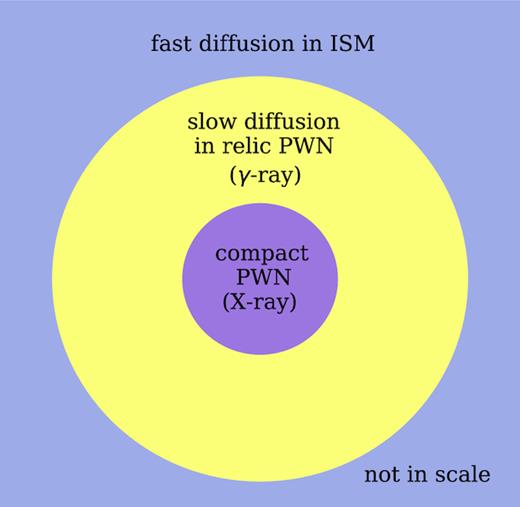
A schematic figure of particle transport in the Geminga PWN. The inner part of the PWN corresponds to the small bow shock nebula detected in X-ray and is unimportant in our model. The outer part of the PWN corresponds to the large nebula detected in γ-ray. Beyond the nebula, particles diffuse isotropically in the ISM where the diffusion coefficient is larger.

The diffusion coefficient in the relic nebula is expected to be smaller than that in the ISM, as the magnetic field in the nebula is higher and the magnetic topology is also more complicated. This naturally explains why the HAWC collaboration derived within the TeV emission region a diffusion coefficient much smaller than the ISM value. We propose that inefficient diffusion in the relic PWN of an old pulsar is likely to be a common phenomenon which can be tested by future γ-ray observation of other nearby pulsars.

4 γ-RAY SPECTRUM OF GEMINGA PWN

We turn now to calculate the IC emission of the Geminga PWN and compare it with the γ-ray data shown in Table 1

4.1 Energy losses

When the electron–positron pairs diffuse in the PWN and the ISM, they lose energy to IC and synchrotron emission. The energy loss rate, including the Klein–Nishina effect, is

\begin{eqnarray*} \dot{E}&=&\dot{E}_{\mathrm{ IC}} +\dot{E}_{\mathrm{ syn}} \nonumber \\ &=& -\frac{4}{3}c\sigma _T \gamma ^2\left[ \sum _i\frac{U_{i}}{(1+4\pi \gamma \epsilon _i)^{3/2}} + \frac{B^2}{8\pi }\right], \end{eqnarray*}

(10)

where c is the speed of light, γ is the electron’s Lorentz factor, and σ_T is the Thomson cross-section. U_i represents the energy density of the radiation field in different energy channel and ε_i is the corresponding normalized photon energy. For a Black Body radiation with a temperature T, we have ε = 2.8K_BT/m_ec², where K_B is the Boltzmann constant and m_e is the electron mass (Moderski et al. 2005). In the calculation, we take into account CMB, infrared (IR), and optical photon fields, which are listed in Table 3. B is the magnetic field due to the central pulsar. The equipartition magnetic field in the X-ray tail close to the pulsar is estimated to be 20μG (Posselt et al. 2017), which implies that the spatial averaged B field within the γ-ray nebula is likely marginally larger than the interstellar value of a few μG. In this work, we adopt B = 3μG in the ISM and assume for simplicity that the cooling in the PWN and ISM is the same.

Table 3.

Physical parameter of the photon fields.

photon field	T(K)	\|$U\rm (eV\,cm^{-3})$\|
CMB	2.7	0.26
IR	20	0.3
Optical	5000	0.3

Table 3.

Physical parameter of the photon fields.

photon field	T(K)	\|$U\rm (eV\,cm^{-3})$\|
CMB	2.7	0.26
IR	20	0.3
Optical	5000	0.3

The cooling time for an electron or positron to decay from E₁ to E₂ via synchrotron and IC emission is

\begin{eqnarray*} \tilde{t}_c(E_1,E_2)&=&\int _{E_2}^{E_1} \frac{-dE}{\dot{E}} \nonumber\\ &=&\int _{E_2}^{E_1} \frac{3dE}{4\gamma ^2\sigma _T c}\left[\frac{B^2}{8\pi }+\sum _i\frac{U_{i}}{(1+4\pi \gamma \epsilon _i)^{3/2}}\right]^{-1}. \end{eqnarray*}

(11)

4.2 IC emission

Based on the conservation of total number of electrons and positrons, the accumulated differential number density of electrons or positrons at time t_age satisfies

\begin{eqnarray*} N(E) = \frac{1}{dE}\int _0^{t_{\mathrm{ age}}}Q(E_0,t_0)\, dE_0\, \mathrm{ d}t_0. \end{eqnarray*}

(12)

A particle with energy E now (i.e. at t_age) was originally injected at t₀ with energy E₀, i.e. |$t_0 = t_{\mathrm{ age}}-\tilde{t}_c(E_0,E)$|⁠. The above integral can be further simplified into

\begin{eqnarray*} N(E) = -\int ^{{\rm min}[E_{hi},\, E_0]}_E \frac{Q[E_0, t_{\mathrm{ age}}-\tilde{t}_c(E_0, E)] }{\dot{E}}\, \mathrm{ d}E_0, \end{eqnarray*}

(13)

if we apply the relation |$\mathrm{ d}t_0/\mathrm{ d}E = -\mathrm{ d}\tilde{t}_c(E_0,E)/\mathrm{ d}E=1/\dot{E}$|⁠. The upper limit of the integration |${\rm min}[E_{hi},\, E_0]$| accounts for the high-energy cut-off of the injection spectrum.

The corresponding IC emission from both electrons and positrons are calculated with the naimapython package (Zabalza 2015), which implements the analytical approximations to IC scattering of blackbody radiation developed by Khangulyan, Aharonian & Kelner (2014). The formula remains accurate within 1 per cent over a wide range of energies.

In Figs 2 and 3, we compare the IC emission of the nebula with the γ-ray data for different injection spectrum and different initial pulsar periods. The upper panel depicts the differential number density E²N(E) of the electrons or positrons, while the lower panel depicts the corresponding IC emission. The MILAGRO, HAWC, and MAGIC data are illustrated with a black square, a circle, and an arrow, respectively. The single power-law model developed in Abeysekara et al. (2017a) overproduces the γ-ray emission in the GeV band even with the corrected MAGIC upper limit. In order to explain the MAGIC upper limit, we need either a broken power-law injection spectrum or a single power-law spectrum but with a larger initial period P₀ as demonstrated in Figs 2 and 3, respectively.

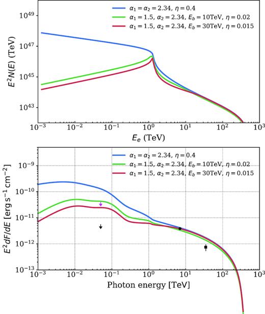
Upper panel: The differential number density E2N(E) as a function of the electron or positron energy for different α1 and α2. Lower panel: IC emission for different injection spectra. The black square and dot denote the MILAGRO and HAWC observations, respectively. The magenta and black arrows describe the corrected and uncorrected MAGIC upper limits, respectively.

Figure 2.

Upper panel: The differential number density E²N(E) as a function of the electron or positron energy for different α₁ and α₂. Lower panel: IC emission for different injection spectra. The black square and dot denote the MILAGRO and HAWC observations, respectively. The magenta and black arrows describe the corrected and uncorrected MAGIC upper limits, respectively.

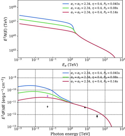
Same as Fig. 2 but for a single power-law injection spectrum with different initial periods P0.

Figure 3.

Same as Fig. 2 but for a single power-law injection spectrum with different initial periods P₀.

In the upper panel, the blue line shows a sharp drop around 1 TeV. This is mainly a reflection of the evolution history of the pulsar spin-down luminosity as indicated in equation (5). Electrons or positrons with energy |$E\gtrsim 1\rm TeV$| have a cooling time |$\tilde{t}_c(E_{\mathrm{ hi}}, E)\lesssim t_{\mathrm{ age}}-\tau _0$| and are injected at t₀ ≳ τ₀ accordingly. τ₀, the initial spin-down time-scale, is much smaller than t_age with the default P₀. When t₀ ≳ τ₀, the pulsar spin-down luminosity decreases rapidly with t₀. Hence, N(E) steepens with energy due to the decrease in the pulsar luminosity. If we increase the initial period P₀, the sharp drop gradually disappears as shown in Fig. 3. This is because τ₀ becomes comparable to t_age and the pulsar spin-down luminosity becomes for a short while a constant in time. P₀ ≳ 0.14 s is required to explain the MAGIC upper limit.

According to Figs 2 and 3, it is difficult to distinguish between the two explanations with only spectral information. The low-energy surface-brightness profile of the nebula is important to disentangle the two possibilities.

5 PARTICLE TRANSPORT AND SPATIAL DISTRIBUTION

We turn now to explore the spatial distribution of the electron–positron pairs and the positron flux on the Earth with a two zone diffusion model. The two zone diffusion model was studied by Fang et al. (2018) recently with numerical simulation. Here, we derive an analytical solution for the model, which involves a slow diffusion in the relic nebula and a fast diffusion in the ISM. The diffusion coefficient in the relic nebula is expected to be smaller than that in the ISM due to the larger magnetic field and the more complicated magnetic field topology.² The two zone diffusion model can explain the small diffusion coefficient derived by Abeysekara et al. (2017a), as it corresponds to the value in the relic nebula instead of the ISM.

To obtain the spatial distribution of the pairs, we solve the particle transport equation

\begin{eqnarray*} \frac{\partial N(E, r, t)}{\partial t}&=&\nabla \cdot \left[D(E, r)\nabla N(E, r,t)\right] \nonumber \\ &&+\,\frac{\partial }{\partial E}\left[\dot{E}(E)N(E,r,t) \right] + Q(E,t)\delta (\vec{r}), \\ \nonumber \end{eqnarray*}

(14)

where D(E, r) is the diffusion coefficient. The source function Q(E, t) and the energy loss term |$\dot{E}(E)$| are defined in equations (8) and (10), respectively. We begin with a discussion of homogeneous diffusion, i.e. a single zone diffusion, and then derive the solution for the two zone case.

5.1 A single zone diffusion

For a homogenous diffusion, Atoyan, Aharonian & Völk (1995) derive an analytical solution for the transport equation

\begin{eqnarray*} N_1(r, E) = \int _{{\rm max}[0,\, t_{\mathrm{ age}}-\tilde{t}_c(E_{hi}, E)]}^{t_{\mathrm{ age}}} \frac{\dot{E}(E_0)}{\dot{E}(E)}\frac{Q(E_0,t_0) }{\pi ^{3/2}r_{\mathrm{ d}}^3}e^{-r^2/r_{\mathrm{ d}}^2} \mathrm{ d}t_0, \end{eqnarray*}

(15)

where E_hi is the high-energy cut-off of the injection spectrum and |$\tilde{t}_c(E_{\mathrm{ hi}}, E)$| is the cooling time from E_hi to E. If E is close to E_hi, the cooling time |$\tilde{t}_c(E_{\mathrm{ hi}},E)$| becomes smaller than t_age. In this situation, only particles injected at |$t_0\gt t_{\mathrm{ age}}-\tilde{t}_c(E_{\mathrm{ hi}}, E)$| contribute to N₁(r, E). This is reflected in the lower limit of the integration. E₀ corresponds to the initial energy of an electron or positron at injection time t₀ that cooled down to E at t_age. r_d is the diffusion length scale which is defined as

\begin{eqnarray*} r_{\mathrm{ d}} = 2 \left[\int _E^{\mathrm{ min}[E_0,E_{\mathrm{ hi}}]}\frac{D(\hat{E})}{\dot{E}(\hat{E})} \mathrm{ d}\hat{E}\right]^{1/2}. \end{eqnarray*}

(16)

In Fig. 4, we plot r_d as a function of E_e for |$t_{\mathrm{ age}}=320\,\rm kyr$|⁠, B = 3μG and

\begin{eqnarray*} D=4.5\times 10^{27}\,\rm cm^2\,s^{-1} \left(\frac{{ \mathit{ E}}}{100\,TeV}\right)^{1/3} \end{eqnarray*}

(17)

for a Kolmogorov-type turbulence.

Figure 4.

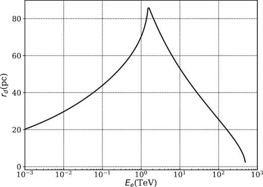
The diffusion length scale r_d, defined in equation (16), as a function of the electron or positron energy with homogeneous diffusion.

|$\dot{E}(E_0)/\dot{E}(E)$| in equation (15) characterizes the energy loss of a particle for an arbitrary cooling function. If there are no energy losses or very slow cooling, then |$\dot{E}(E_0)/\dot{E}(E) \rightarrow 1$| and equation (15) recovers the solution with no energy loss, i.e.

\begin{eqnarray*} N_{1,nl}(r, E) = \int _{0}^{t_{\mathrm{ age}}} \frac{Q(E,t) }{\pi ^{3/2}r_{\mathrm{ d}}^3}e^{-r^2/r_{\mathrm{ d}}^2} \mathrm{ d}t. \end{eqnarray*}

(18)

In equation (15), the term

\begin{eqnarray*} H_1(r,E)=\frac{1}{\pi ^{3/2}r_{\mathrm{ d}}^3}e^{-r^2/r_{\mathrm{ d}}^2} \end{eqnarray*}

(19)

describes the spatial distribution of all the particle. If integrated over the whole space, equation (15) simply recovers the spectral energy distribution derived in equation (13).

5.2 Two zone diffusion

We assume now a diffusion coefficient of the form

\begin{eqnarray*} D(E, r)=\left(\frac{E}{100 \,\rm TeV}\right)^{1/3}\left\lbrace \begin{array}{@{}l@{\quad }l@{}}D_1, \, 0 \,\lt\, r\,\lt\, r_{\mathrm{ b}},\\ D_2, \, r\,\ge\, r_{\mathrm{ b}}, \end{array}\right. \end{eqnarray*}

(20)

where r_b is the boundary between the two zones. For simplicity we fix r_b = 60 pc and then vary D₁ to reproduce the HAWC surface-brightness profile (Abeysekara et al. 2017a). After obtaining D₁, we vary D₂ and compare the results with the positron excess data. r_bis expected to be ≳30 pc, otherwise we cannot reproduce the HAWC surface-brightness profile. If r_b is too large, then the positron flux on the Earth becomes similar to the single zone model result and it cannot account for the positron excess. The exact value of r_b can be constrained by future multiwavelength observation.

To derive the solution for two zone diffusion, we only need to replace the homogeneous diffusion term H₁(r, E) in equation (15) with the two zone diffusion term H₂(r, E). The solution now becomes

\begin{eqnarray*} N_2(r, E) = \int _{{\rm max}[0,\, t_{\mathrm{ age}}-\tilde{t}_c(E_{hi}, E)]}^{t_{\mathrm{ age}}} \frac{\dot{E}(E_0)}{\dot{E}(E)}Q(E_0,t_0) H_2(r,E) \mathrm{ d}t_0, \end{eqnarray*}

(21)

where

\begin{eqnarray*} H_{2}(r,E) = \frac{ b(b+1)}{\pi ^{3/2}r_{d1}^3[\rm 2b^2erf(r_b)-b(b-1)erf(2r_b)+2erfc(r_b)]} \end{eqnarray*}

\begin{eqnarray*} \times \left\lbrace \begin{array}{@{}l@{\quad }l@{}}\left[e^{-r^2/r_{\mathrm{ d}1}^2} + \left(\frac{b-1}{b+1}\right)\left(\frac{2r_\mathrm{ b}}{r}-1\right)e^{-(r-2r_{\mathrm{ b}})^2/r_{\mathrm{ d}1}^2} \right], \, r\lt r_\mathrm{ b},\\ \left(\frac{2b}{b+1}\right)\left[\frac{r_\mathrm{ b}}{r}+b(1-\frac{r_\mathrm{ b}}{r})\right]e^{-[(r-r_{\mathrm{ b}})/r_{\mathrm{ d}2}+r_{\mathrm{ b}}/r_{\mathrm{ d}1}]^2}, \, r\ge r_\mathrm{ b}.\\ \end{array}\right.&& \end{eqnarray*}

(22)

b, r_d1 and r_d2 are constants and are defined as

\begin{eqnarray*} b\equiv \frac{\sqrt{D_1}}{\sqrt{D_2}}, \end{eqnarray*}

(23)

\begin{eqnarray*} r_{\mathrm{ d}1}(E) \equiv 2 \left[\int _E^{\mathrm{ min}(E_0,E_{\mathrm{ hi}})}\frac{D(x,r\lt r_\mathrm{ b})}{\dot{E}(x)} \mathrm{ d}x\right]^{1/2} \end{eqnarray*}

(24)

and

\begin{eqnarray*} r_{\mathrm{ d}2}(E) \equiv 2 \left[\int _E^{\mathrm{ min}(E_0,E_{\mathrm{ hi}})}\frac{D(x,r\gt r_\mathrm{ b})}{\dot{E}(x)} \mathrm{ d}x\right]^{1/2}, \end{eqnarray*}

(25)

respectively. erf(x) is the error function and erfc(x) = 1 – erf(x). Appendix A describes a detailed derivation of H₂(r, E).

|$r_{\mathrm{ d}1}^3 H_2(r,E)$| is a dimensionless quantity, which depends on three dimensionless parameter r/r_d1, b, and r_b/r_d1. Here, we are interested in the regime with b < 1 and r_b/r_d1 ≳ 1. Since the diffusion coefficient in the ISM is expected to be larger than that in the nebula. Under the assumption of r_b = 60 pc, the diffusion length scale presented in Fig. 4 satisfies r_d1 ≲ r_b for the entire energy range.

In the upper panel of Fig. 5, we fix b and then investigate how does the spatial distribution of H₂ vary with r_b/r_d1. As r_b/r_d1 increases the resulting profile gradually approaches the single zone solution. This is mainly because when r_b ≫ r_d1, the source is unable to feel the second zone. In the lower panel, we fix r_b/r_d1 and study how does H₂ vary with b. For a given ratio of r_b/r_d1, when b decreases, particles can diffuse further away from the source. This helps to explain the observed positron excess. The effect is mainly important for the particles with r_d1 ≈ r_b = 60 pc, i.e. particles with energy around a few TeV (see Fig. 4). H₂ approaches zero at small r/r_d1 values because we adopt an absorption boundary at the source. It is not clear what should be the appropriate condition at the inner boundary. But we expect that the inner boundary condition has only small effects on the large-scale structure like the positron flux on the Earth.

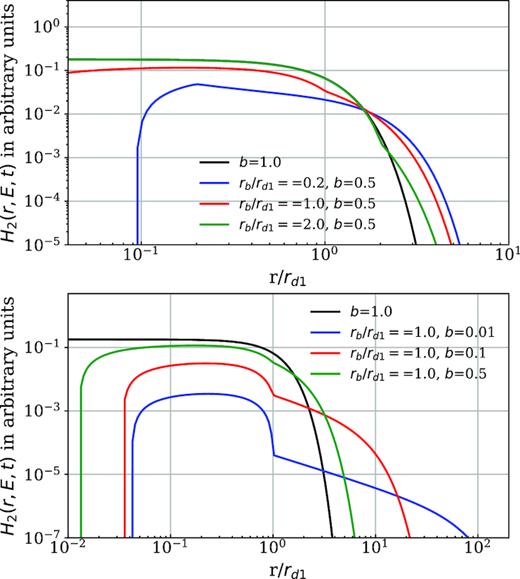
The two zone diffusion term H2(r, E, t) defined in equation (22) as a function of the dimensionless length scale r/rd1 for different combinations of b and rb/rd1. The black solid line is the result from a single zone diffusion with b = 1.

Figure 5.

The two zone diffusion term H₂(r, E, t) defined in equation (22) as a function of the dimensionless length scale r/r_d1 for different combinations of b and r_b/r_d1. The black solid line is the result from a single zone diffusion with b = 1.

5.3 The surface brightness

Integrating N₂(r, E) along the line of sight and then calculating the corresponding IC emission, we obtain the γ-ray surface-brightness profile of the Geminga PWN (see Fig. 6). We neglect the finite size of the nebula, which may introduce at most an effect of |$(r_{\mathrm{ d}}/d)^2\lt 10{{\ \rm per\ cent}}$|⁠. To simplify the calculation, we also approximate

\begin{eqnarray*} r_{\mathrm{ d}}(E)\approx 2\left[\frac{D(E) E}{(1-\delta)\dot{E}}\right]^{1/2}\left[1 - \left(\frac{E}{E_0}\right)^{1-\delta }\right]^{1/2}. \end{eqnarray*}

(26)

and

\begin{eqnarray*} E_0(E, \tilde{t}_\mathrm{ c})\approx \frac{E}{1-\dot{E} \tilde{t}_\mathrm{ c} /E}, \end{eqnarray*}

(27)

where |$\tilde{t}_\mathrm{ c}$| is the cooling time since injection.

Figure 6.

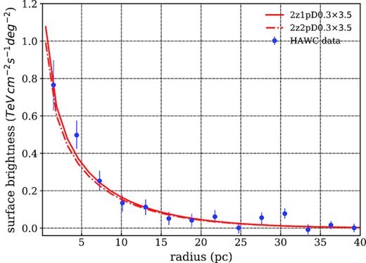
Surface-brightness profiles between 5 and 50 TeV of the photon energy. The HAWC data are taken from Abeysekara et al. (2017a) and the HAWC model is calculated with the same parameter as in Abeysekara et al. (2017a). 2z1pD03 and 2z2pD03 are the single power-law and broken power-law model, respectively.

In Fig. 6, we compare the HAWC data with different model results. The physical paramters applied in the different models are listed in Table 4. The ‘HAWC’ model is calculated with the same parameter as in Abeysekara et al. (2017a). ‘2z1pDx’ stands for a two zone diffusion model with a single power-law injection spectrum and D₁/D₂ = x, while ‘2z2pDx’ denotes two zone diffusion model with a broken power-law injection spectrum and D₁/D₂ = x. Since we adopt r_b = 60 pc, which is larger than the size of observed γ-ray nebula, the two zone diffusion model produces almost the same surface-brightness profile as the single zone model within r_b. Within the two zone model the surface-brightness profile at radius r ≲ 20 pc is insensitive to the D₁/D₂ ratio. Hence, models with D₁/D₂ = 0.05 and 0.01 are not plotted in Fig. 6.

Table 4.

Model parameter.

Model name	α₁	α₂	E_b (TeV)	\|$D_1(10^{27}\,\rm cm^2\,s^{-1}$\|⁠)	D₁/D₂	r_b(pc)	P₀ (s)	η	B (μG)	E_min (TeV)	E_max(TeV)
HAWC	2.34	2.34	–	4.5	1	–	0.045	0.4	3	10⁻³	500
2z1pD03	2.34	2.34	–	4.5	0.3	60	0.14	0.4	3	10⁻³	500
2z1pD005	2.34	2.34	–	4.5	0.05	60	0.14	0.4	3	10⁻³	500
2z1pD001	2.34	2.34	–	4.5	0.01	60	0.14	0.4	3	10⁻³	500
2z2pD03	1.5	2.34	30	4.5	0.3	60	0.045	0.015	3	10⁻³	500
2z2pD005	1.5	2.34	30	4.5	0.05	60	0.045	0.015	3	10⁻³	500
2z2pD001	1.5	2.34	30	4.5	0.01	60	0.045	0.015	3	10⁻³	500

Model name	α₁	α₂	E_b (TeV)	\|$D_1(10^{27}\,\rm cm^2\,s^{-1}$\|⁠)	D₁/D₂	r_b(pc)	P₀ (s)	η	B (μG)	E_min (TeV)	E_max(TeV)
HAWC	2.34	2.34	–	4.5	1	–	0.045	0.4	3	10⁻³	500
2z1pD03	2.34	2.34	–	4.5	0.3	60	0.14	0.4	3	10⁻³	500
2z1pD005	2.34	2.34	–	4.5	0.05	60	0.14	0.4	3	10⁻³	500
2z1pD001	2.34	2.34	–	4.5	0.01	60	0.14	0.4	3	10⁻³	500
2z2pD03	1.5	2.34	30	4.5	0.3	60	0.045	0.015	3	10⁻³	500
2z2pD005	1.5	2.34	30	4.5	0.05	60	0.045	0.015	3	10⁻³	500
2z2pD001	1.5	2.34	30	4.5	0.01	60	0.045	0.015	3	10⁻³	500

Note. D₁ is at 100 TeV.

Table 4.

Model parameter.

Model name	α₁	α₂	E_b (TeV)	\|$D_1(10^{27}\,\rm cm^2\,s^{-1}$\|⁠)	D₁/D₂	r_b(pc)	P₀ (s)	η	B (μG)	E_min (TeV)	E_max(TeV)
HAWC	2.34	2.34	–	4.5	1	–	0.045	0.4	3	10⁻³	500
2z1pD03	2.34	2.34	–	4.5	0.3	60	0.14	0.4	3	10⁻³	500
2z1pD005	2.34	2.34	–	4.5	0.05	60	0.14	0.4	3	10⁻³	500
2z1pD001	2.34	2.34	–	4.5	0.01	60	0.14	0.4	3	10⁻³	500
2z2pD03	1.5	2.34	30	4.5	0.3	60	0.045	0.015	3	10⁻³	500
2z2pD005	1.5	2.34	30	4.5	0.05	60	0.045	0.015	3	10⁻³	500
2z2pD001	1.5	2.34	30	4.5	0.01	60	0.045	0.015	3	10⁻³	500

Model name	α₁	α₂	E_b (TeV)	\|$D_1(10^{27}\,\rm cm^2\,s^{-1}$\|⁠)	D₁/D₂	r_b(pc)	P₀ (s)	η	B (μG)	E_min (TeV)	E_max(TeV)
HAWC	2.34	2.34	–	4.5	1	–	0.045	0.4	3	10⁻³	500
2z1pD03	2.34	2.34	–	4.5	0.3	60	0.14	0.4	3	10⁻³	500
2z1pD005	2.34	2.34	–	4.5	0.05	60	0.14	0.4	3	10⁻³	500
2z1pD001	2.34	2.34	–	4.5	0.01	60	0.14	0.4	3	10⁻³	500
2z2pD03	1.5	2.34	30	4.5	0.3	60	0.045	0.015	3	10⁻³	500
2z2pD005	1.5	2.34	30	4.5	0.05	60	0.045	0.015	3	10⁻³	500
2z2pD001	1.5	2.34	30	4.5	0.01	60	0.045	0.015	3	10⁻³	500

Note. D₁ is at 100 TeV.

We multiply our results by a factor of 3.5 when comparing the HAWC data. It is because when we apply the same parameter as in Abeysekara et al. (2017a), we found that the resulting γ-ray flux is consistent with the value based on the disc template,³ see the supplementary fig. 2 in Abeysekara et al. (2017a). The surface-brightness data however appear to agree with the value estimated with a diffusion template, which is larger than the disc template’s value by a factor about 3.5. This discrepancy will not affect the discussion with broken power-law injection spectrum, as we can simply increases the acceleration efficiency by the same factor. Larger γ-ray flux of the Geminga PWN does make it difficult for the model with a single power-law injection spectrum to interpret the surface-brightness data as the current η = 0.4.

5.4 The positron flux at the Earth

Fig. 7 depicts the number density of positrons, N₂(r, E), as a function of the radius r at energy E = 1 TeV. We focus on two different situations, a single power-law injection spectrum with a larger initial period P₀ and a broken power-law spectrum with a smaller P₀. This is illustrated in the upper panel and the lower panel, respectively. The basic parameters for all the different models are listed in Table 4.

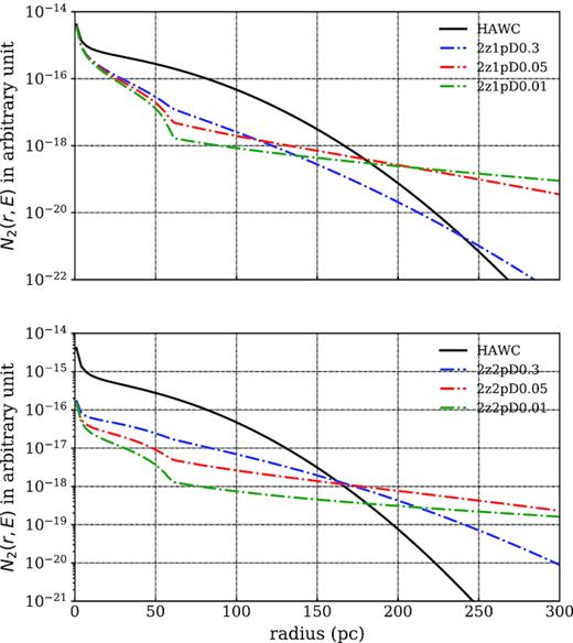
$The differential number density of positron (or electron), N2(r, E), as a function of distance r at energy $E=1\,$ TeV. A single power law with a larger initial period P0 (upper panel). A broken power-law injection spectrum with a smaller P0 (lower panel). The black solid line represents the model from Abeysekara et al. (2017a).$

Figure 7.

The differential number density of positron (or electron), N₂(r, E), as a function of distance r at energy |$E=1\,$| TeV. A single power law with a larger initial period P₀ (upper panel). A broken power-law injection spectrum with a smaller P₀ (lower panel). The black solid line represents the model from Abeysekara et al. (2017a).

When the D₁/D₂ ratio decreases, the positron flux at the Earth (assuming d = 250 pc) increases as the Earth position is shifted from the exponential tail to the plateau region in the spatial distribution (see Fig. 7). The positron flux reaches a maximum at D₁/D₂ ∼ 0.05 and it is boosted by more than 2 orders of magnitude compared with the single zone model results. When the D₁/D₂ ratio decreases further, the positron flux at the Earth decreases as the normalization constant of the plateau region becomes smaller.

Fig. 8 depicts the positron spectrum produced by the Geminga pulsar at the Earth for the different models shown in Fig. 7. The single power-law model produces a flat positron spectrum at Earth, which seems to be more consistent with data.⁴ However, the broken power-law model cannot be ruled out. If D₁/D₂ ∼ 0.05, both the single power-law model and the broken power-law model can contribute a significant fraction of the positron excess above ∼300 GeV. It is worth noting that all the models discussed here are not meant to be the best fit for the positron flux data but mainly for illustration. As it is difficult to explore the whole parameter space. Future γ-ray observations in the GeV band will enable us to put strong constraints on the model set up and narrow the parameter space. Positron flux from other nearby pulsars also need to be investigated in future study.

Figure 8.

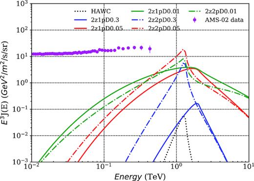
The positron flux at the Earth produced by the Geminga pulsar with different model setup listed in Table 4.

With D₁/D₂ = 0.05, the diffusion coefficient in the ISM is found to be

\begin{eqnarray*} D_{\mathrm{ ISM}}\sim 2\times 10^{27}\,\rm cm^2\,s^{-1} \left(\frac{E}{1\,GeV}\right)^{1/3}, \end{eqnarray*}

(28)

which is still 1 order of magnitude smaller than the standard value but more consistent with the low value required in the spiral arm model (Benyamin et al. 2014). For a given average path-length, CRs experience a lower average interaction with the ISM in the spiral arm model than in the standard CR model. In order to recover the observed secondary to primary ratio, the spiral arm model requires a smaller halo of about a few hundred pc to keep the CRs closer to the galactic plane where the density is higher. The smaller halo requires a lower diffusion coefficient in the ISM which is estimated to be |${\sim } 10^{27}\, \rm cm^2\,s^{-1}$| at 1 GeV (Shaviv et al. 2009). The two zone diffusion model studied here seems to support the spiral arm model.

5.5 The proper motion of the Geminga pulsar

The Geminga pulsar has a transverse velocity of |$v_t \approx 211 (d/250\rm pc) \rm \, km s^{-1}$| (Faherty et al. 2007). The corresponding transverse distance travelled by the pulsar in t_age is estimated to be

\begin{eqnarray*} d_{t}=v_t t_{\mathrm{ age}}\sim 70\, {\rm pc}\, \left(\frac{d}{250\, {\rm pc}}\right)\left(\frac{t_{\mathrm{ age}}}{ 320\,\rm kyr}\right). \end{eqnarray*}

(29)

The displacement d_t introduced by the pulsar proper motion is comparable to the spatial extension of the TeV nebula detected by HAWC (Abeysekara et al. 2017a). This may affect the γ-ray morphology of the PWN. The radial velocity of the Geminga pulsar is unclear but it is likely smaller than its transverse velocity, otherwise the bow shock nebula will not be revealed clearly in X-ray due to projection effect (Caraveo et al. 2003, 2004; Posselt et al. 2017).

As a first attempt to investigate the effect of the proper motion, we focus on the simple single zone diffusion model. The two zone diffusion model requires knowledge of the time and spatial evolution of the PWN, which is beyond the scope of this work. According to Section 2.2, we choose that the pulsar is at the origin O(0, 0, 0) now and it was moving along the x-axis with a transverse velocity of |$v_t \approx 211\,\rm km\,s^{-1}$|⁠. The y-axis is perpendicular to the proper motion in the plane of sky, while the z-axis is along the line of sight. The birth place of the pulsar then is simply at (−d_t, 0, 0), where d_t = v_tt_age ≈ 70 pc. The differential number density in equation (15) is modified into

\begin{eqnarray*} N_1(x,y,z,E) &=& \int _{{\rm max}[0,\, t_{\mathrm{ age}}-\tilde{t}_c(E_{hi}, E)]}^{t_{\mathrm{ age}}} \frac{\dot{E}(E_0)}{\dot{E}(E)}\frac{Q(E_0,t_0) }{\pi ^{3/2}r_{\mathrm{ d}}^3} \nonumber \\ &&\times \, e^{-[(x+v_{t}t_{\mathrm{ age}}-v_{t}t_0)^2+y^2+z^2]/r_{\mathrm{ d}}^2}\, \mathrm{ d}t_0, \end{eqnarray*}

(30)

where v_t is the traverse velocity of the pulsar.

The proper motion of the Geminga pulsar is mainly important for the surface-brightness profile of the PWN at low energies E_e ≲ 1 TeV. In the TeV band, the morphology of the nebula is found to be not strongly affected by the proper motion. Because the corresponding electron–positron pairs have a smaller lifetime and the corresponding transverse motion of the pulsar is smaller than that estimated in equation (29). It is consistent with the roughly spherical symmetric nebula revealed in the HAWC observations (Abeysekara et al. 2017a). In the lower energy band, where the lifetime of electrons–positron pairs are close to t_age, a bow shock nebula morphology is instead expected, and indeed observed in X-rays (Caraveo et al. 2003). In Fig. 9, we present the surface-brightness profile of the Geminga PWN between 50 and 100 GeV that is relevant for the MAGIC band with the set-up of the HAWC model. The nebula is elongated in the negative x-direction due to the proper motion. Within the single zone model, the proper motion of the pulsar has a limited influence on the positron flux at Earth, as it only changes the distance of the pulsar slightly introducing an effect |${\lesssim } (v_tt_{\mathrm{ age}}/d)^2 \approx 10{{\ \rm per\ cent}}$|⁠.

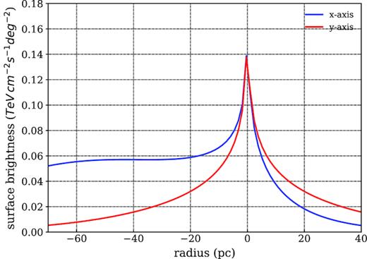
$The surface-brightness profile between 50 and $100\,$ GeV (i.e. the MAGIC band) both along the proper motion direction (x-axis) and perpendicular to the proper motion direction in the plane of sky (y-axis).$

Figure 9.

The surface-brightness profile between 50 and |$100\,$| GeV (i.e. the MAGIC band) both along the proper motion direction (x-axis) and perpendicular to the proper motion direction in the plane of sky (y-axis).

10.1088/0004-637X/700/2/L127

6 DISCUSSION

We propose that the γ-ray emission detected by HAWC and MILAGRO in the direction of Geminga originated from the relic PWN surrounding the pulsar. We developed a two zone diffusion model with a slow diffusion D₁ in the PWN and a fast diffusion D₂ in the ISM. This model would explain both the surface-brightness profile and the positron excess ≳300 GeV. With D₁/D₂ ∼ 0.05, the Geminga pulsar can supply a significant fraction of the positron excess above ∼300 GeV. The diffusion coefficient in the ISM is |$D_{\mathrm{ ISM}}\sim 2\times 10^{27}\,\rm cm^2\,s^{-1} (\mathit{ E}/1\,GeV)^{1/3}$|⁠. This value is one order of magnitude smaller than the standard value but more consistent with the low value required in the spiral arm model for the CR propagation (e.g. Shaviv et al. 2009).

There are several factors that can affect the γ-ray emission and the surface-brightness profile of the Geminga PWN and the positron flux at Earth. The MAGIC upper limit implies either a broken power-law injection spectrum or a single power law but with a larger initial period P₀. This can be tested by future multiwavelength observation. We assume that the particle acceleration efficiency η is a constant. If instead η gradually decreases with time, then our calculation underestimates the positron flux from the Geminga pulsar. This helps to relieve the discrepancy between the HAWC detection (Abeysekara et al. 2017a) and the idea that the Geminga pulsar is a main source of the positron excess. The proper motion of the Geminga pulsar was studied with a single zone model. We found that a bow shock nebula morphology likely has appeared in the GeV emission. This can be tested by future MAGIC observation.

The main caveat of our model is that we neglect the dynamical evolution of the PWN and focus only on the time evolution of the pulsar spin-down power. In other words, we investigate a model with a dynamical pulsar and a static nebula with time-independent diffusion coefficient and magnetic field. The peak of the positron flux on the Earth corresponds to the pairs injected at an early phase of the Geminga pulsar, when the pulsar spin-down luminosity was still large. Therefore, the understanding of the diffusion of TeV pairs in young PWNe, like the Crab, is crucial for explaining the observed positron excess at ≳300 GeV. The slow diffusion revealed by Abeysekara et al. (2017a) in the γ-ray emission region instead characterizes the properties of the relic nebula at the late phase and is likely irrelevant.

In young PWN like the Crab with an age of a few thousand years, the diffusion coefficient of TeV positrons is found to be |${\sim } 5\times 10^{26}\,\rm cm^{2}\,s^{-1}$| through a spectral index fitting of the synchrotron emission⁵ (Tang & Chevalier 2012). The corresponding escape time is estimated to be

\begin{eqnarray*} t_{\mathrm{ esc}}\sim \frac{R^2}{4D_{\mathrm{ PWN}}} \sim 150\, \rm yr\, \left(\frac{R}{1\,\rm pc}\right)^2 \left(\frac{5\times 10^{26} \,\rm cm^2\,s^{-1}}{D_{PWN}}\right). \end{eqnarray*}

(31)

In the early phase of the pulsar evolution, the nebula is small and t_esc is much smaller than the age of the Geminga pulsar t_age. The diffusion time of TeV positrons in the ISM is approximately the age of the pulsar, i.e. t_age = d²/4D_ISM. This implies

\begin{eqnarray*} D_{\mathrm{ ISM}} \sim \frac{d^2}{4t_{\mathrm{ age}}}\sim 1.5\times 10^{28}\,{\rm cm^2\,s^{-1}}\, \left(\frac{d}{250 \,\rm pc}\right)^2 \left(\frac{320 \,\rm kyr}{t_{\mathrm{ age}}}\right) \end{eqnarray*}

(32)

at 1 TeV, where d is the distance of the pulsar. If we assume a Kolmogorov-type turbulence, then the diffusion coefficient in the ISM becomes |$1.5\times 10^{27}\,\rm cm^2\,s^{-1} (\mathit{ E}/1\,GeV)^{1/3}$|⁠, which again is more consistent with the value required by the spiral arm model. Based on the above discussion, the time evolution of PWNe can affect the positron flux on the Earth. This will be addressed in future work.

In summary, by considering a physically motivated PWN model for the γ-ray observation of HAWC and MILAGRO we have shown that the Geminga pulsar is a good candidate to be source of a significant fraction of the observed positron excess at ≳300 GeV .

ACKNOWLEDGEMENTS

We thank Nir Shaviv and Reetanjali Moharana for helpful discussions. The research was supported by an ERC advanced grant TReX and by the CHE-ISF I-CORE center for excellence.

Footnotes

1

Note however that in the standard model ad hoc re-acceleration or winds are needed to explain the very low-energy behaviour (Strong et al. 2007).

2

Note that for simplicity when calculating the cooling we take the magnetic field to be the same in the PWN and in the ISM

3

The HAWC data shown in Figs 2 and 3 are based on the disc template.

4

Note that in the spiral arm model the pulsars contribute only to the higher end of the excess.

5

Note we extend the diffusion coefficient provided in table 3 of Tang & Chevalier (2012) to 1 TeV with a Komogorov-type energy dependence.

REFERENCES

Abdo

A. A.

et al. ,

2009

,

ApJ

,

700

,

L127

Abeysekara

A. U.

et al. ,

2017

,

Science

,

358

,

911

10.1126/science.aan4880

Abeysekara

A. U.

et al. ,

2017

,

ApJ

,

843

,

40

10.3847/1538-4357/aa7556

10.1103/PhysRevLett.108.011103

Ackermann

M.

et al. ,

2012

,

Phys. Rev. Lett.

,

108

,

011103

10.1103/PhysRevLett.105.121101

Adriani

O.

et al. ,

2010

,

Phys. Rev. Lett.

,

105

,

121101

10.1103/PhysRevLett.110.141102

Aguilar

M.

et al. ,

2013

,

Phys. Rev. Lett.

,

110

,

141102

10.1051/0004-6361/201527722

Ahnen

M. L.

et al. ,

2016

,

A&A

,

591

,

A138

Atoyan

A. M.

,

Aharonian

F. A.

,

Völk

H. J.

,

1995

,

Phys. Rev. D

,

52

,

3265

10.1103/PhysRevD.52.3265

10.1088/0004-637X/782/1/34

Benyamin

D.

,

Nakar

E.

,

Piran

T.

,

Shaviv

N. J.

,

2014

,

ApJ

,

782

,

34

10.3847/0004-637X/826/1/47

Benyamin

D.

,

Nakar

E.

,

Piran

T.

,

Shaviv

N. J.

,

2016

,

ApJ

,

826

,

47

Bertsch

D. L.

et al. ,

1992

,

Nature

,

357

,

306

10.1038/357306a0

10.1146/annurev.astro.34.1.331

Bignami

G. F.

,

Caraveo

P. A.

,

1996

,

ARA&A

,

34

,

331

10.3847/0004-637X/817/2/129

Bîrzan

L.

,

Pavlov

G. G.

,

Kargaltsev

O.

,

2016

,

ApJ

,

817

,

129

Brisken

W. F.

,

Thorsett

S. E.

,

Golden

A.

,

Goss

W. M.

,

2003

,

ApJ

,

593

,

L89

10.1086/378184

Caraveo

P. A.

,

Bignami

G. F.

,

De Luca

A.

,

Mereghetti

S.

,

Pellizzoni

A.

,

Mignani

R.

,

Tur

A.

,

Becker

W.

,

2003

,

Science

,

301

,

1345

10.1126/science.1086973

Caraveo

P. A.

,

Bignami

G. F.

,

De Luca

A.

,

Pellizzoni

A.

,

Mereghetti

S.

,

Mignani

R. P.

,

Tur

A.

,

Becker

W.

,

2004

,

Mem. Soc. Astron. Italiana

,

75

,

470

Chandrasekhar

S.

,

1943

,

Rev. Mod. Phys.

,

15

,

1

10.1103/RevModPhys.15.1

de Luca

A.

,

Caraveo

P. A.

,

Mattana

F.

,

Pellizzoni

A.

,

Bignami

G. F.

,

2006

,

A&A

,

445

,

L9

10.1103/PhysRevD.98.063017

Evoli

C.

,

Linden

T.

,

Morlino

G.

,

2018

,

Phys. Rev. D

,

98

,

063017

10.1007/s10509-007-9368-0

Faherty

J.

,

Walter

F. M.

,

Anderson

J.

,

2007

,

Ap&SS

,

308

,

225

Fang

K.

,

Bi

X.-J.

,

Yin

P.-F.

,

Yuan

Q.

,

2018

,

ApJ

,

863

,

30

10.1146/annurev.astro.44.051905.092528

Gaensler

B. M.

,

Slane

P. O.

,

2006

,

ARA&A

,

44

,

17

Halpern

J. P.

,

Holt

S. S.

,

1992

,

Nature

,

357

,

222

10.1038/357222a0

10.1146/annurev.astro.45.051806.110608

Hester

J. J.

,

2008

,

ARA&A

,

46

,

127

10.1088/1475-7516/2009/01/025

Hooper

D.

,

Blasi

P.

,

Dario Serpico

P.

,

2009

,

J. Cosmol. Astropart. Phys.

,

1

,

025

10.1103/PhysRevD.89.063539

Ibarra

A.

,

Lamperstorfer

A. S.

,

Silk

J.

,

2014

,

Phys. Rev. D

,

89

,

063539

10.1088/0004-637X/783/2/100

Kargaltsev

O.

,

Rangelov

B.

,

Pavlov

G. G.

,

2013

,

preprint (arXiv:1305.2552)

Khangulyan

D.

,

Aharonian

F. A.

,

Kelner

S. R.

,

2014

,

ApJ

,

783

,

100

López-Coto

R.

,

Giacinti

G.

,

2018

,

MNRAS

,

479

,

4526

10.1093/mnras/sty1821

Miyazawa

T.

,

Izuyama

T.

,

1987

,

Phys. Rev. A

,

36

,

5791

10.1103/PhysRevA.36.5791

10.1111/j.1365-2966.2005.09494.x

Moderski

R.

,

Sikora

M.

,

Coppi

P. S.

,

Aharonian

F.

,

2005

,

MNRAS

,

363

,

954

10.3847/1538-4357/835/1/66

Posselt

B.

et al. ,

2017

,

ApJ

,

835

,

66

10.1103/PhysRevD.97.123008

Profumo

S.

,

Reynoso-Cordova

J.

,

Kaaz

N.

,

Silverman

M.

,

2018

,

Phys. Rev. D

,

97

,

123008

10.1103/PhysRevLett.103.111302

Shapiro

S. L.

,

Teukolsky

S. A.

,

1983

,

Black Holes, White Dwarfs, and Neutron Stars: The Physics of Compact Objects

.

Wiley-Interscience

,

New York

, p.

663

Google Scholar

Google Preview

OpenURL Placeholder Text

WorldCat

Shaviv

N. J.

,

Nakar

E.

,

Piran

T.

,

2009

,

Phys. Rev. Lett.

,

103

,

111302

10.1146/annurev.nucl.57.090506.123011

Strong

A. W.

,

Moskalenko

I. V.

,

Ptuskin

V. S.

,

2007

,

Ann. Rev. Nucl. Part. Sci.

,

57

,

285

10.1088/0004-637X/752/2/83

Tang

X.

,

Chevalier

R. A.

,

2012

,

ApJ

,

752

,

83

10.1088/0004-637X/755/1/39

Verbiest

J. P. W.

,

Weisberg

J. M.

,

Chael

A. A.

,

Lee

K. J.

,

Lorimer

D. R.

,

2012

,

ApJ

,

755

,

39