The imprint of clump formation at high redshift – I. A disc α-abundance dichotomy Free

ABSTRACT

1 INTRODUCTION

The Milky Way (MW) is important to our understanding of the structure and evolution of galactic discs. The geometical thick disc was originally discovered in the MW by decomposing the vertical star count profile into two components, the thin and thick discs (Yoshii 1982; Gilmore & Reid 1983). Spectroscopic studies of Solar neighborhood stars found that the thick disc is composed of mainly older (∼12–7 Gyr) stars that are enhanced in their α abundances, while thin-disc stars are younger (<7 Gyr) and have near-Solar α abundances (e.g. Fuhrmann 1998; Haywood et al. 2013). Bovy et al. (2012) studied the spatial distribution of mono-abundance populations which showed smooth variations of scale height with abundance and suggested that there was no distinct separation of ‘geometrical’ discs (Bovy, Rix & Hogg 2012), nor, perhaps, in chemistry. Even so, the ‘chemical’ separation of high- and low-α populations persists in recent high-resolution abundance surveys such as APOGEE (e.g. Anders et al. 2014; Nidever et al. 2014; Hayden et al. 2015) and unbiased Solar neighborhood samples (Adibekyan et al. 2012).

It is now believed that the chemically and geometrically defined thick discs are different entities. The chemically defined thick disc has a shorter scale length than the geometric thick disc (Robin et al. 1996; Ojha 2001; Jurić et al. 2008; Bensby et al. 2011; Bovy et al. 2012; Martig et al. 2016), although there is still some uncertainty about the scale lengths (Robin et al. 2014). Old, α-enhanced stars are concentrated to the inner MW (Minchev et al. 2015). Stars in the chemical thick disc are generally old, whereas geometric thick disc stars can have median ages as young as |$5{\:{\rm Gyr}}$| in the outer disc (Martig et al. 2016).

Several explanations have been proposed for the α-bimodality. The ‘two-infall’ model (Chiappini, Matteucci & Gratton 1997; Chiappini 2009; Grisoni et al. 2017) suggests that the early MW had a high star formation rate (SFR) (short gas consumption time-scale) that changed dramatically around 8 Gyr when there was a drop in the overall MW SFR and a large infall of pristine gas that diluted the overall metallicity of the MW and gave rise to the thin disc, low-α population. Since this model requires a particular event to occur (the large infall of pristine gas at a particular time), it suggests that the bimodality might not be a generic feature of all galaxies.

On the other hand, a ‘superposition’ model [which is similar to the scenario proposed in Schönrich & Binney (2009)] postulates that the α-bimodality is a generic consequence of the chemical and dynamical processes in a spiral disc galaxy. The chemical evolution in α abundance is quite rapid at early times but slows down at later times when most of the stars are formed. In addition, a radial gradient in outflow rate exists in the disc due to the decrease in the energy required to unbind the gas. The large outflow in the outer disc inhibits the gas from attaining a high metallicity while in the inner galaxy chemical evolution is able to advance fairly unimpeded. Finally, the dynamical process of radial migration then moves stars away from their birth radii and thereby smoothes out the separate chemical evolution tracks. The α-bimodality is created by the fact that the chemical evolution proceeds most quickly as SNIa’s turn on and evolution is moved from high-α to low-α thus producing fewer stars in the α ‘valley’. Producing chemical bimodality via these processes requires fine-tuning; indeed simulations which include these processes have failed to produce any chemical bimodality (e.g. Loebman et al. 2011; Minchev, Chiappini & Martig 2013), which instead only produce a thick band in the ([α/Fe], [Fe/H]) space representing the overall chemical evolution of the galaxy with small variations with radius. Nidever et al. (2014) present a detailed discussion and example figures of the chemical evolution of these two scenarios.

Nevertheless, in recent years some simulations have begun to find hints of α-bimodalities. The AURIGA simulations have found α-bimodalities produced by an early centralized starbust (important for the inner galaxy) and disc contraction (important for the outer galaxy) that produce chemical bimodalities somewhat similar to the MW in one of six simulated galaxies (Grand et al. 2017). Others have found that a late infall of a gas-rich galaxy can produce some metal-poor, α-poor stars that give rise to a bimodality (Snaith et al. 2016; Mackereth et al. 2018). However, these bimodalities are weaker than the one observed in the MW and the age distributions are not always consistent with the MW, suggesting they are not the main mechanism at work in the MW.

One option that has not been previously considered is the influence of star-forming ‘clumps’. Clumps are commonly found in Hubble Space Telescope (HST) images of high-redshift galaxies (e.g. Elmegreen & Elmegreen 2005; Ravindranath et al. 2006; Elmegreen et al. 2007; Förster Schreiber et al. 2011; Genzel et al. 2011; Guo et al. 2012, 2015). Such clumps were first identified by eye in HST images (e.g. Cowie, Hu & Songaila 1995; van den Bergh et al. 1996) and are common in MW progenitors at high redshift (present in |${\sim } 55{{\ \rm per\ cent}}$| of such galaxies at a redshift of 3, Guo et al. 2015). They appear |${\sim } 1 {\:{\rm kpc}}$| in size when observed at low resolution, but at higher resolution appear to have sizes from |$100{\:{\rm pc}}$| to |$500{\:{\rm pc}}$| (Livermore et al. 2012, 2015; Fisher et al. 2017; Cava et al. 2018). Clumps can contribute up to |$20{{\ \rm per\ cent}}$| of the integrated SFR of a galaxy, but can be less massive (up to |$7{{\ \rm per\ cent}}$| of the total mass, Wuyts et al. 2012). It is proposed that they form a bulge in less than half a Gyr (Dekel, Sari & Ceverino 2009). They have also been proposed for the origin of the geometrical thick disc (Bournaud, Elmegreen & Martig 2009).

In this paper, we demonstrate that discs evolving with significant clump formation produce a bimodality in the [α/Fe]-[Fe/H] space by virtue of the very rapid star formation which occurs in clumps. We show that the resulting high-α track in chemical space is comprised of old stars and suggest that this might be the process forming the α-bimodality in the MW. The layout of this paper is as follows: in Section 2, we describe the simulation we use in this paper. Section 3 then presents the results of the simulation. We present our conclusions in Section 4.

2 SIMULATION

We set up a spherical Navarro–Frenk–White (Navarro, Frenk & White 1997) halo with an equilibrium spherical gas distribution containing 10 per cent of the total mass and following the same density distribution. The starting halo is set up as described in Roškar et al. (2008): it has a mass within the virial radius (r₂₀₀ ≃ 200 kpc) of 10¹² M_⊙. A temperature gradient ensures an initial gas pressure equilibrium for an adiabatic equation of state. Gas velocities are initialized to give a spin parameter of λ = 0.065 (Bullock et al. 2001; Macciò et al. 2007), with specific angular momentum j ∝ R, where R is the cylindrical radius. Both the gas corona and the dark matter halo are comprised of 10⁶ particles; gas particles initially have masses 1.4 × 10⁵ M_⊙ and force softening 50 pc. Dark matter particles instead come in two mass flavours (10⁶ M_⊙ and 3.5 × 10⁶ M_⊙ inside and outside 200 kpc, respectively), with a softening of 100 pc. The stars in the simulation form self-consistently out of cooling gas, inheriting the softening and chemistry of the parent gas particle.

We evolve the simulation for 10 Gyr with gasoline (Wadsley, Stadel & Quinn 2004; Wadsley, Keller & Quinn 2017), the smooth particle hydrodynamics (SPH) extension of the N-body tree-code pkdgrav (Stadel 2001). Gas cooling includes the metal-line cooling implementation of Shen, Wadsley & Stinson (2010); in order to prevent the cooling from dropping below the resolution of our simulation, we set a pressure floor on gas particles p_floor = 3Gε²ρ², where G is Newton’s gravitational constant, ε is the softening length, and ρ is the gas particle’s density (Agertz, Teyssier & Moore 2009). Gas cools and settles into a disc; once the density exceeds 1cm⁻³ and the temperature drops below 15 000 K, star formation and supernova feedback cycles are initiated as described in Stinson et al. (2006). A consequence of the metal cooling is that gas can reach lower temperatures where it is prone to fragmentation and clump formation. Supernovae feedback couples 10 per cent of the 10⁵¹ erg per supernova to the interstellar medium as thermal energy. We include the effects of turbulent diffusion (Shen et al. 2010) allowing the gas to mix, reducing the scatter in the age–metallicity relation (Pilkington et al. 2012). We use a base time step of Δt = 10 Myr with time steps refined such that |$\delta t = \Delta t/2^n \lt \eta \sqrt{\epsilon /a_g}$|⁠, where a_g is the acceleration at a particle’s position and the refinement parameter η = 0.175. We set the opening angle of the tree-code gravity calculation to θ = 0.7. In addition the time step of gas particles satisfies the condition δt_gas = η_couranth/[(1 + α)c + βμ_max], where η_courant = 0.4, h is the SPH smoothing length set over the nearest 32 particles, α and β are, respectively, the linear and quadratic viscosity coefficients and μ_max is described in Wadsley et al. (2004). Star particles represent single stellar populations with a Miller–Scalo initial mass function. SNII and SNIa yields of oxygen and iron are taken from Raiteri, Villata & Navarro (1996). As in Raiteri et al. (1996), Padova stellar lifetimes are used to determine SNII rates, and SNIa rates are determined from those same lifetimes in a binary evolution model.

2.1 Global properties of the final system

Fig. 1 presents the face-on and edge-on views of the model at the end of the simulation, showing it to be a reasonable example of a disc galaxy. Fig. 2 presents the final rotation curve and velocity dispersions of the system. While our simulation is not designed to match any specific galaxy, the rotation curve of the final system has a circular velocity at |$8 {\:{\rm kpc}}$| of |$242\,{\:{\rm km\, s^{-1}}}$|⁠, making it comparable to the MW. Its structural and kinematic properties are somewhat different from the MW’s, for instance the model is unbarred, but is otherwise similar enough that it can be used to understand the origin of trends observed in the MW.

Figure 1.

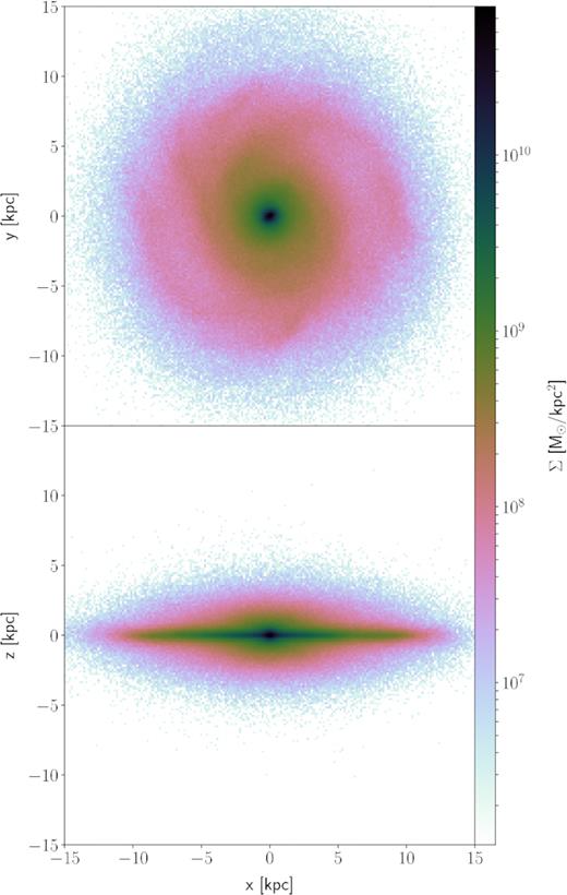
Stellar density of the final model viewed face-on (top) and edge-on (bottom).

Open in new tabDownload slide

Figure 2.

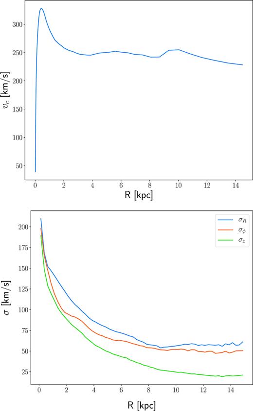
Top: Rotation curve of the final model. Bottom: Velocity dispersion profiles of all stars in different directions of the final model.

Open in new tabDownload slide

3 RESULTS

3.1 Chemical bimodality

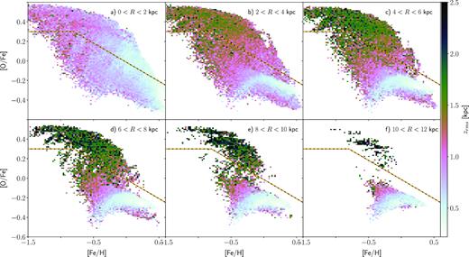
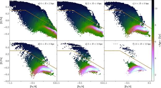
Fig. 3 shows the final (⁠|$10{\:{\rm Gyr}}$|⁠) distribution of stars in the |$\rm [O/Fe]$|-|$\rm [Fe/H]$| (chemical) plane at different radii and heights. As in the APOGEE survey (Anders et al. 2014; Nidever et al. 2014; Hayden et al. 2015) and other data sets (e.g. Fuhrmann 1998; Bensby et al. 2005; Reddy, Lambert & Allende Prieto 2006; Adibekyan et al. 2012), we find two distinct sequences, a high-α and a low-α one. The low-α sequence dominates over the high-α one close to the mid-plane, while the high-α sequence is more prominent at larger heights. The two sequences are bridged by stripes which are not observed in the MW. If we convolve the |$\rm [O/Fe]$| and |$\rm [Fe/H]$| of stellar particles in the Solar neighbourhood (defined throughout this paper as 7 < R/kpc < 9) with the APOGEE observational errors, |${\sigma _{{\rm [Fe/H]}}} = 0.1$| dex and |${\sigma _{{\rm [O/Fe]}}} = 0.03$| dex (Nidever et al. 2014) the stripes visible in Fig. 3 are masked, without erasing the chemical bimodality. Fig. 4 directly shows the bimodality in |$\rm [O/Fe]$| at the Solar neighbourhood for the cut through the chemical space |$-0.5 \lt {\rm [Fe/H]}\lt -0.4$|⁠. The distribution is bimodal, with a very clearly defined minimum, even when the distribution is convolved with the observational errors, as it must be.

Figure 3.

[O/Fe]-[Fe/H] distributions of the simulation for various radial and height cuts, as labelled in each panel. The dashed yellow–black line, defined by equation (1), separates the the high-α and low-α sequences. Each panel is normalized to a total weight of unity.

Open in new tabDownload slide

Figure 4.

Histograms of |$\rm [O/Fe]$| for the sample at |$-0.5 \lt {\rm [Fe/H]}\lt -0.4$|⁠. The cyan histogram shows the raw distribution from the model while the orange histogram shows the bimodality persists when noise typical of APOGEE is added to each star’s chemistry.

Open in new tabDownload slide

Fig. 5 compares the chemical distribution in the MW as observed by APOGEE throughout a large extent of the galaxy (DR14 red giants, Holtzman et al. 2018) with that of the model convolved with the APOGEE observational errors. The lower sequence has the opposite curvature compared with the model but this may be sensitive to the star formation history (SFH) and the specific elements used (e.g. Ramírez, Allende Prieto & Lambert 2007), as is the scale of the vertical axis. The |$\rm [\alpha /Fe]$| defined by APOGEE includes oxygen but also other α-elements; when we consider just |$\rm [O/Fe]$| in the APOGEE data, although the two sequences are noisier, the curvature of the low-α track is similar to the simulation’s at the low |$\rm [Fe/H]$| end, though still opposite at high |$\rm [Fe/H]$|⁠. None the less, an unambiguous and sustained separation into two tracks is readily apparent in the model, as in the MW. Additionally, the extent and curvature of the upper sequence is similar to that in the APOGEE data. The facts that the high-α sequence covers nearly the same |$\rm [Fe/H]$| range as the low-α sequence, and that the two sequences approach each other at the high |$\rm [Fe/H]$| end, are especially intriguing constraints on the formation of the bimodality because it implies that the high-α sequence did not form in a single discrete event such as infall of pristine gas (e.g. Mackereth et al. 2018). The extension of the high-α sequence to lower metallicities than the low-α also matches the MW. Still, the model and the MW do not match in detail; one of the more significant differences is the larger separation between the high-α and the low-α sequences. This may be a problem of either the yields used (also supported by the relative vertical offset of the model and the MW) or the SFRs that produce the high-α sequence.

Figure 5.

Chemical comparison with APOGEE data. On the left-hand panel is the model chemistry in the |$\rm [O/Fe]$|-|$\rm [Fe/H]$| space convolved with APOGEE-like uncertainties, while the right-hand panel presents the chemistry of red giant stars in the APOGEE survey (DR14) in the |$\rm [\alpha /Fe]$|-|$\rm [Fe/H]$| space.

Open in new tabDownload slide

3.2 Present day properties of the high-α sequence

The spatial distribution of the high-α stars is also evident in Fig. 3. High-α stars are more prominent at large heights at the present time. The high-α distribution is also more centrally concentrated than the low-α ones; in the MW Bovy et al. (2012) found shorter scale lengths for low-α stars while Hayden et al. (2015) found little evidence of the high-α sequence outside the Solar neighbourhood. Fig. 6 shows the present-day root-mean-square vertical height of stars across the chemical space. The high-α stars are distributed in a thicker disc than the low-α stars outside the bulge region (e.g. Bovy et al. 2012). The variation of height is continuous across the chemical space, as found in the MW by Bovy et al. (2012). This important constraint suggests that the high-α stars are not the product of a single violent event that had suddenly heated the disc vertically. In spite of this continuous height variation the vertical stellar density profile is very clearly double-exponential, as can be seen in Fig. 7 for the Solar neighbourhood (other regions in the disc look qualitatively similar). Fitting two exponentials to the Solar neighbourhood vertical profile of the model gives scale heights |$h_1 = 240 \pm 8{\:{\rm pc}}$| and |$h_2 = 1083 \pm 52{\:{\rm pc}}$|⁠; in comparison Jurić et al. (2008) measured |$h_1 = 300\pm 50{\:{\rm pc}}$| and |$h_2 = 900 \pm 180{\:{\rm pc}}$| in the Solar neighbourhood. The geometric thin and thick discs have a transition at about |$1{\:{\rm kpc}}$|⁠, which is comparable to the transition in the MW (e.g. Gilmore & Reid 1983).

Figure 6.

Root-mean-square height, z_rms, of stars in chemical space for various radial cuts, as labelled in each panel. We suppress bins with less than 10 star particles. The dashed yellow–black line, defined by equation (1), separates the two sequences.

Open in new tabDownload slide

Figure 7.

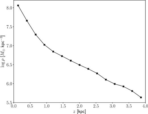
The model’s vertical density distribution in the Solar neighbourhood.

Open in new tabDownload slide

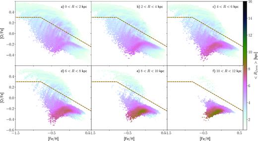
Nidever et al. (2014) and Hayden et al. (2015) showed that the metallicity distribution function (MDF) of α-enhanced stars is essentially independent of the location within the MW’s disc. Fig. 8 presents the MDFs of stars with |${\rm [O/Fe]}\gt 0.2$| [note this α-enhanced population is not identical to the high-α sequence, but is chosen in the same spirit as in Nidever et al. (2014)], in the simulation for various radial and height cuts. The overall shape and width of these MDFs are similar in all regions considered. Nidever et al. (2014) and Hayden et al. (2015) suggested that the similarity of the MDFs of α-enhanced stars indicates these stars formed from well-mixed gas. Loebman et al. (2016) used simulations to demonstrate that the similarity of the MDF of α-enhanced stars is due to them having formed in a relatively small region in the inner Galaxy over a short time interval (⁠|$\lesssim 2{\:{\rm Gyr}}$|⁠) and were subsequently migrated throughout the disc. Fig. 9 presents the average age of stars in the chemical space. The high-α stars are old, having mean age |$\gt 8 {\:{\rm Gyr}}$|⁠, while the low-α stars, particularly those at high |$\rm [Fe/H]$|⁠, are predominantly young to intermediate age. Fig. 10 presents the mean formation radius, R_form, across the chemical space. The high-α stars largely formed within the inner |$2 {\:{\rm kpc}}$|⁠, while the low-α stars formed over a larger radial region. In agreement with Loebman et al. (2016) therefore we find that the high-α stars, and especially the α-enhanced stars, formed over a short time interval in a relatively restricted volume.

Figure 8.

MDFs of the α-enhanced stars (here defined as |${\rm [O/Fe]}\gt 0.2$|⁠) at different radii (indicated by different colours) and different heights above the mid-plane (as indicated in each panel). The MDFs of this population are homogenous across the galaxy.

Open in new tabDownload slide

Figure 9.

Mean age of stars in the chemical space for various radial cuts, as labelled in each panel. We suppress bins with less than 10 star particles. The dashed yellow–black line, defined by equation (1), separates the two sequences.

Open in new tabDownload slide

Figure 10.

Mean radius of formation, R_form, of stars in the chemical space for various radial cuts, as labelled in each panel. We suppress bins with less than 10 star particles. The dashed yellow–black line, defined by equation (1), separates the two sequences.

Open in new tabDownload slide

Fig. 11 shows the SFH of the high-α and low-α stars. The two populations overlap at old ages, with the SFH of the high-α stars peaking very early, persisting to |${\sim } 4{\:{\rm Gyr}}$|⁠, but largely over by |$2{\:{\rm Gyr}}$|⁠. The SFH of the low-α stars is relatively flat after |$1{\:{\rm Gyr}}$|⁠, becoming the main mode of star formation thereafter. The early formation of the majority of the high-α stars ensures that they are more centrally concentrated than the subsequent low-α disc stars, in good agreement with what is found in the MW (Bovy et al. 2012, 2016).

Figure 11.

The SFH of the two sequences across the entire model. The (red) triangles show the high-α sequence while the (blue) downward-pointing triangles show the low-α sequence. The (black) circles show the total SFH.

Open in new tabDownload slide

Fig. 12 compares the stellar ages in the MW from the APOGEE survey and the simulation. The left-hand panel, showing the ages in the simulation, uses star particles in the simulation with |$|z| \lt 1 {\:{\rm kpc}}$|⁠, and across Galactic radii similar to the red clump (⁠|$3 \lt x \lt 13{\:{\rm kpc}}$| and |$|y| \gt 5{\:{\rm kpc}}$|⁠). The right-hand panel uses ∼20 000 red clump stars in APOGEE with ages from Ness et al. (2016). While ages of the high-α stars are similar between the model and the MW, the two are quite different in detail. The biggest difference is at low metallicity, where the model has young stars only at low α. The model’s chemical enrichment history therefore is different from that of the MW. This makes the similarities in the bimodality even more remarkable.

Figure 12.

Age comparison with APOGEE data. On the left-hand panel is the model’s mean stellar age in |$\rm [O/Fe]$|-|$\rm [Fe/H]$| space, while the right-hand panel presents the mean age of stars in APOGEE in the |$\rm [\alpha /Fe]$|-|$\rm [Fe/H]$| space.

Open in new tabDownload slide

3.3 Two modes of star formation

We now investigate in greater detail the origin of the high-α sequence. High-α stars are generally thought to form at high SFR; we compute the local SFR density, Σ_SFR, at birth of each star particle from the distribution of stars forming in each |$10 {\:{\rm Myr}}$| interval. We estimate the density of these new stars by recovering their positions at the beginning of the time interval using the mean disc rotation velocity at their radius. We then calculate the density of the particles in the disc plane by binning the particles in Cartesian coordinates with a bin size of 100 × 100 pc. The grid is then smoothed with a Gaussian of full width at half-maximum, FWHM|$=200 {\:{\rm pc}}$| and the values are converted to physical units of |$\:{\rm M_{\odot }}{\:{\rm yr}}^{-1} {\:{\rm kpc}}^{-2}$|⁠. Finally, we assign local Σ_SFR values to each star particle on the basis of the bin within which it falls.

Fig. 13 presents snapshots of the local SFR computed this way over the course of the simulation. At early times a considerable amount of star formation occurs in clumps, which have a high SFR density. As in the two-infall model of Chiappini et al. (1997) this mode of star formation becomes negligble after a few Gyr, aside from at the bulge. At the same time as the clumpy star formation is occurring, stars are forming in the disc in a more distributed (‘smooth’) configuration with much lower Σ_SFR. This is the main mode of star formation after |$3{\:{\rm Gyr}}$|⁠.

Figure 13.

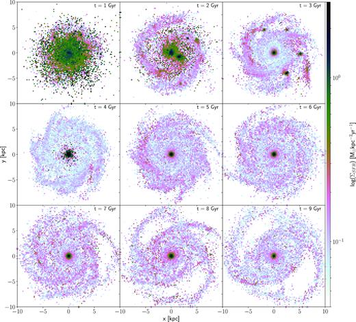
Maps of the SFR computed as described in the text. The panels are spaced by |$1 {\:{\rm Gyr}}$| from |$t=1{\:{\rm Gyr}}$| (top left) to |$9{\:{\rm Gyr}}$| (bottom right). While low Σ_SFR ‘smooth’ star formation occurs throughout the galaxy at all times, there is high Σ_SFR clumpy star formation only during the first few Gyr. Each panel shows the distribution of stars younger than |$200{\:{\rm Myr}}$|⁠; during this time some high-α stars will have diffused out of their birth clumps. This is particularly evident at |$t=1{\:{\rm Gyr}}$|⁠.

Open in new tabDownload slide

Fig. 14 shows Σ_SFR of star particles at the time of formation across the chemical plane. The high-α sequence has a significantly higher Σ_SFR, which results in being α-rich, while the low-α stars have much lower local Σ_SFR and chemically evolve more slowly. Unlike Fig. 6, Fig. 14 has an abrupt transition between the high-α and the low-α sequences. Fig. 15 presents histograms of Σ_SFR at formation, showing that there is a bimodality in Σ_SFR. The two modes of SF differ by a factor of roughly 100 in Σ_SFR. The high-α sequence forms via the high-SFR density, clumpy star formation mode, while the low-α sequence forms via the low-SFR density, smooth star formation mode that is dominant at later times. As already shown in Fig. 11, the low-α mode of star formation is already present at early times at the same time as the high SFR, high-α mode. This simultaneous formation of both α-sequences, via the dual-modes of star formation, appears to be in agreement with the recent observational results of Silva Aguirre et al. (2018) and Hayden et al. (2017).

Figure 14.

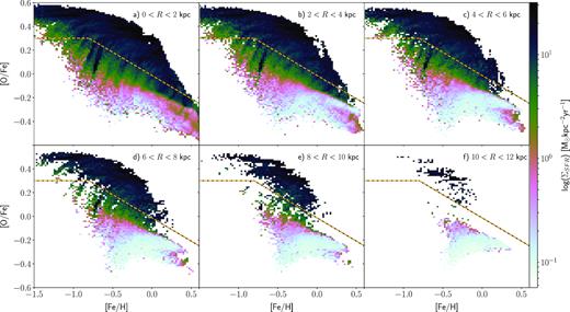
The mean Σ_SFR of star particles in the chemical abundance plane in various spatial bins. The high-α stars have high Σ_SFR while low-α stars have low Σ_SFR. The dashed yellow–black line, defined by equation (1), separates the two sequences. We suppress bins with less than 10 star particles.

Open in new tabDownload slide

Figure 15.

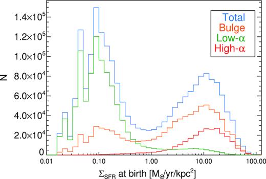
Histogram of Σ_SFR for all star particles. This shows a bimodality in Σ_SFR with a minimum at intermediate SFRs. The low-α and high-α histograms are obtained for all stars outside |$R \gt 2 {\:{\rm kpc}}$|⁠, whereas the bulge distribution is for stars at |$R \lt 2 {\:{\rm kpc}}$|⁠. The bimodality is not produced by stars at the bulge.

Open in new tabDownload slide

Fig. 16 shows the evolution of the radius at which stars are forming in the high-α and low-α sequences. The high-α sequence is seen to derive from a decreasing number of discrete star-forming clumps that sink towards the centre. The star formation in the low-α sequence is more broadly distributed, although the effect of spirals is evident as gaps in the radial distribution at |$R_f \lt 3{\:{\rm kpc}}$| at certain times. These spirals are associated with the clumps, by being partly excited by them (D’Onghia, Vogelsberger & Hernquist 2013) and also partly needing the density enhancement provided by spirals to assemble the gas needed to form clumps. Low-α star formation is also associated with the clumps throughout a large fraction of their trajectories, but the bulk of low-α stars form outside clumps, particularly after the first Gyr. A similar plot to Fig. 16 but separated into a low and high SFR density at |$\Sigma _\mathrm{SFR} = 30\:{\rm M_{\odot }}{\:{\rm kpc}}^{-2}{\:{\rm yr}}^{-1}$| is virtually identical apart from having more star formation in the bulge, persisting for the full |$10{\:{\rm Gyr}}$|⁠. About |$43{{\ \rm per\ cent}}$| of stars form in the high SFR density component, which reduces to |$31{{\ \rm per\ cent}}$| if the inner |$0.5{\:{\rm kpc}}$| is excluded. In comparison we earlier found that the high-α sequence comprised |$28{{\ \rm per\ cent}}$| of all stars. Comparing these two numbers we conclude that the majority of high-α stars form at high Σ_SFR within clumps.

Figure 16.

The evolution of the radius at which stars form for the high-α (top) and low-α (bottom) sequences over the first |$4{\:{\rm Gyr}}$|⁠.

Open in new tabDownload slide

Fig. 17 presents the evolution of two typical clumps chosen by eye. Clump 1 forms at |${\sim } 6{\:{\rm kpc}}$|⁠; initially on the low-α sequence, it quickly shoots up to the high-α sequence as Σ_SFR rises, becoming more |$\rm [Fe/H]$|-rich along this sequence as supernovae of type Ia commence. Its orbit decays and by the time it reaches |$1{\:{\rm kpc}}$| it starts falling back on to the low-α sequence. At this point the clump is lost in the bulge. Clump 2 also ascends from the low-α to the high-α sequence. Its orbital radius is rather more constant, and it evolves in |$\rm [Fe/H]$| less over its shorter lifetime (⁠|$300{\:{\rm Myr}}$| versus |$500{\:{\rm Myr}}$| in clump 1). Towards the end of its life it merges with another clump and quickly drops to the centre of the galaxy, dropping from the high-α to the low-α sequence. These two clumps illustrate an important point: contrary to the usual interpretation, the high-α sequence is reached from the low-α sequence, rather than forming before it. These examples also demonstrate that the stripes connecting the low-α to the high-α sequence are due to the evolution of individual clumps in chemical space.

Figure 17.

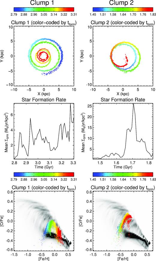
The evolution of two clumps in configuration space (top), SFR density (middle), and chemical space (bottom). Clump 1 (left-hand panels) forms around |$2.8 {\:{\rm Gyr}}$| and over the next |$0.5{\:{\rm Gyr}}$| sinks to the centre. During this time it quickly transitions from the low-α to the high-α sequence. Clump 2 (right-hand panels) behaves similarly but towards the end of its life it merges with another clump and quickly falls to the centre. Colour codes for the time, as indicated by the wedges. In the bottom row, the grey scale indicates the distribution of all stars at the end of the simulation.

Open in new tabDownload slide

The clump mass distribution is shown in Fig. 18. Clumps are detected in 100 Myr snapshots using a 10σ threshold in the 100 × 100 pc binned mass map with a 1.5 kpc smoothed background removed. The total clump mass is measured by summing up the mass in a |$500 {\:{\rm pc}}$| radius around the clump centre and removing the background level determined in a |$1.5\!-\!2.5 {\:{\rm kpc}}$| annulus. Only clumps with well-determined masses (error |${\lesssim }10{{\ \rm per\ cent}}$|⁠; to remove noise fluctuations) and galactocentric radii greater than |$100 {\:{\rm pc}}$| (to remove the inner bulge) are kept and these correspond well to the visually identifiable clumps. Note that because clumps survive for |${\sim }500 {\:{\rm Myr}}$| before falling into the galactic centre, they are detected multiple times in our technique. The range of clump masses is from 3 × 10⁷ to 8 × 10⁹ M_⊙ with a mean of 5 × 10⁸ M_⊙, although our detection technique is not sensitive to clumps below ∼3 × 10⁷. This mean mass is of the same order, but higher than the median clump mass found in high-redshift galaxies observed at high resolution through gravitational lensing, 10⁸ M_⊙, (e.g. Cava et al. 2018, their fig. 2).

Figure 18.

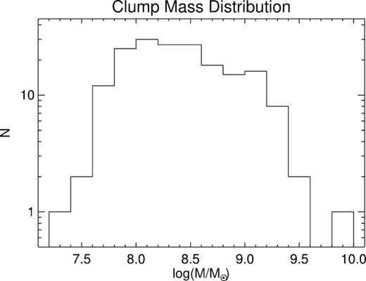
The distribution of clump masses which ranges from ∼3 × 10⁷ to 10¹⁰ M_⊙.

Open in new tabDownload slide

3.4 A high-redshift view

The images from dart-ray are noise-free and have a spatial resolution comparable to that of the simulation. To enable a better comparison with real observations, we degrade the signal-to-noise and spatial resolution of the images to that typical of high-redshift surveys (see also Snyder et al. 2015). Therefore, we generate synthetic Hubble Space Telescope Wide Field Camera 3 (HST/WFC3) images matched to the observing conditions of the CANDELS (Grogin et al. 2011) and HUDF09 (Bouwens et al. 2010) surveys, adopting the typical depth and resolution of these surveys as listed in Table 1 of Guo et al. (2013). We create synthetic HST/WFC3 images for three WFC3 filters – F098M, F125W, and F160W. At z = 2, these trace 0.3–0.5 |$\mu$|m in the rest frame, i.e. UV, B, and V band. To generate the synthetic images, we first rescale the surface brightness of each pixel as I_observed = I_emitted × (1 + z)⁻⁴ to account for cosmological surface brightness dimming, ignoring k-corrections. The angular sizes of the pixels are then scaled with the redshift and the pixels are rebinned to 0.6 arcsec pixel⁻¹ – the typical pixel scale of drizzled HST WFC3 observations. Next, we convolve the images with a 2D Gaussian kernel to simulate the WFC3 point spread function, FWHM 0.13 arcsec for F098M and 0.16 arcsec for F125W and F160W. Finally, we add shot noise to each pixel to match the typical depth of each survey – 5σ limits of ∼27.5 and 28.3 mag arcsec⁻² for the wide and deep portions of the CANDELS survey, respectively, and 29.7 mag arcsec⁻² for the HUDF09.

Fig. 19 shows the resulting images, at the original resolution, and convolved with HST resolution, with surface brightness dimming included and with noise added as in the CANDELS survey (Grogin et al. 2011) and the Hubble Ultra Deep Field (HUDF, Beckwith et al. 2006). We use these images to identify clumps. We first fit a single-component Sérsic (Sérsic 1968) model to the F098M image (0.3 |$\mu$|m rest wavelength) and search in the residual image for off-centre clumps. Following the definition of Guo et al. (2018), we identify one clump containing |${\sim } 14{{\ \rm per\ cent}}$| of the total UV flux in the CANDELS-wide image. This clump, visible in the top right of the galaxy, is comprised of four sub-clumps which merge together at this resolution. It is at |$4 {\:{\rm kpc}}$| from the galaxy centre at this time and has a F098M-F160W (U − V rest wavelength) colour of 0.34 ± 0.15, which is significantly bluer than the rest of the galaxy, but within the range of observed clumps (e.g. Guo et al. 2018). Our analysis of the mock deep and ultradeep images identifies three additional mini-clumps, having less than |$1{{\ \rm per\ cent}}$| of the total UV flux and would not be considered clumps in the usual definition. Their U − V colours range from 0.2 to 0.8.

Figure 19.

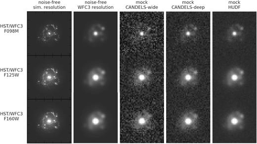
The model at |$t = 1 {\:{\rm Gyr}}$| as it would appear at z = 2 if viewed by HST. The left column shows the full high-resolution images produced by the radiative transfer calculations, while the remaining columns convolve these images to the WFC3 resolution and add noise as in CANDELS and HUDF.

Open in new tabDownload slide

We have repeated this analysis at |$t=2{\:{\rm Gyr}}$| and at |$t=3{\:{\rm Gyr}}$| (still pretending that the galaxy is at z = 2). At |$t=2{\:{\rm Gyr}}$| we find two clumps, each contributing |${\sim } 10{{\ \rm per\ cent}}$| of the UV flux, while we find only one clump and only at the UDF depth for |$t=3{\:{\rm Gyr}}$|⁠, contributing |${\sim } 9{{\ \rm per\ cent}}$| of the UV flux.

This analysis shows that our simulation is not plagued by an excess clump formation and would not be viewed as unusual if found amongst galaxies at z ∼ 2.

4 DISCUSSION AND CONCLUSIONS

We have shown that the early, gas-rich phase of galaxy formation, which supports two modes of star formation, distributed and clumpy, as generally observed by HST at high redshift, naturally gives rise to a bimodal distribution in chemical space, similar to what is seen in the MW. The clumpy mode of star formation has an SFR density about 100 times higher than the distributed mode and leads to rapid self-enrichment with high α-abundance, whereas the distributed star formation is responsible for less α-enchanced stars. As the stellar mass of the galaxy builds up, the gas fraction drops, leading to less star formation taking place in clumps, which naturally shuts off most of the formation of high-α stars (with star formation in the bulge being the exception).

While the vertical distribution of stars in Figs 6 and 7 is reminiscent of the thick disk in the MW, the density distribution of high-α stars flares, which means there is not a direct one-to-one match between our model and the MW. The high-α vertical scale height is consistent with MW observations at larger radii, but it is too small in the inner galaxy to match the MW. This inconsistency could be a result of the idealized nature of our simulation, which is isolated and thus excludes the effects of galaxy accretion that would dynamically heat the disc (and increase the scale height) further and is most important at early times, when most of the high-α stars are forming. The inclusion of these effects would bring our model into closer agreement with the observations. Moreover, the age of stars in chemical space are qualitatively different from those in the MW, although this affects the low-α sequence (the ‘thin’ disc) more than the high-α one. The main result we highlight here is the fact that the current simulation is naturally able to produce the chemical bimodality that is seen in the surveys but which, to date, has been challenging to produce in simulations.

Clumps are thought to form via gravitational instability in gas-rich discs (Noguchi 1999; Immeli et al. 2004; Elmegreen, Bournaud & Elmegreen 2008; Inoue et al. 2016), although some clumps may have an ‘ex situ’ (merger) origin (e.g. Puech et al. 2009; Hopkins et al. 2013; Mandelker et al. 2014). The fate of clumps in simulations has been a subject of debate, with either their destruction by supernova and/or radiative feedback (Genel et al. 2012; Hopkins et al. 2012; Buck et al. 2017; Oklopčić et al. 2017) or sinking to the centre of the galaxy to contribute to the bulge (Noguchi 1999; Immeli et al. 2004; Bournaud, Elmegreen & Elmegreen 2007; Elmegreen et al. 2008; Genzel et al. 2008; Dekel et al. 2009; Ceverino, Dekel & Bournaud 2010; Mandelker et al. 2017) suggested. We have found that our clumps sink to the centre of the galaxy on time-scales of 200–500 Myr. In a companion paper, we explore the consequences of clumps falling to the centre for the chemistry of the bulge, which further helps constrain this model.

We have verified that if we increase the supernova feedback in our simulations that clump formation is substantially inhibited and no chemical bimodality results. Although we use a lower feedback efficiency than is often employed in cosmological simulations, we have demonstrated that the clumps in our simulation are reasonable compared to observations, such as those in the CANDELS-wide (Grogin et al. 2011) and the HUDF (Beckwith et al. 2006), and that our model is not excessively clumpy. At present there is some uncertainty regarding the overall importance of clumps; our results suggest that even with modest clumps the chemical consequences for the MW could be significant.

Recently Mackereth et al. (2018) suggested that a bimodality in chemical space can be produced through gas accretion. Their cosmological simulations produce chemical bimodality in about 5% of the time for L_* galaxies. In contrast, the scenario presented here will work for a large fraction of galaxies with mass comparable to the MW; Wuyts et al. (2012) find that |${\sim } 40{{\ \rm per\ cent}}$| of galaxies of MW mass are clumpy at 1.5 < z < 2.5 when considering their mass distribution (rising to |$60{{\ \rm per\ cent}}$| in the UV) in which case most such galaxies will have chemical bimodalities. At the moment this prediction cannot be tested but future facilities, such as the Extremely Large Telescope, Giant Magellan Telescope, and the Thirty Meter Telescope, may be able to map the chemical space of stars in nearby galaxies.

4.1 Summary

The results and implications of this study are as follows:

• We produce a bimodal distribution of stars in the |$\rm [O/Fe]$|-|$\rm [Fe/H]$| space via clumpy + distributed star formation. The clumps self-enrich in α-elements due to their high SFR density and produce the high-α sequence while the low-α sequence is produced by the distributed star formation. The clumpy mode becomes less efficient as the gas mass fraction drops, leaving an α-enhanced population that is old at the present day. The clumps produced in our simulation are in reasonable agreement with clumps observed at z ∼ 2 (e.g. Guo et al. 2018).

• Clumps form on the low-α sequence, and ascend to the high-α sequence and their SFR increases. Towards the ends of their lives, they tend to drop back to the low-α sequence, although this typically happens close to the bulge.

• The two α-sequences form simultaneously early on in the evolution of the MW, resulting in overlapping ages. Recent results by Silva Aguirre et al. (2017) and Hayden et al. (2017) indicate that temporal overlap of the two sequences is seen in the observations as well. For the foreseeable future this age overlap is the most promising way to test this hypothesis further.

• The model predicts that bimodal chemical thick discs should be common at the mass of the MW, since at least |${\sim } 40{{\ \rm per\ cent}}$| of galaxies of MW mass are clumpy at z ∼ 2 (Wuyts et al. 2012). An important test of this scenario therefore is that chemical bimodality should be common in MW mass galaxies.

The importance of clumps to the evolution of disc galaxies continues to be hotly debated (e.g. Ceverino et al. 2010; Hopkins et al. 2012; Moody et al. 2014; Tamburello et al. 2015; Mayer et al. 2016; Buck et al. 2017; Mandelker et al. 2017; Tamburello et al. 2017; Benincasa et al. 2018). The lifetimes and masses of clumps are therefore somewhat uncertain, and in simulations is dependent on resolution and sub-grid physics (e.g. Tamburello et al. 2015), and possibly also on the mode of gas accretion (Ceverino et al. 2010). However there is a growing view from high-redshift observations that clumps cannot be too massive given the high degree of rotation in discs (e.g. Wuyts et al. 2012; Wisnioski et al. 2015, 2018). For instance, by seeding their models with a spectrum of velocity perturbations matching the turbulent cascade, Benincasa et al. (2018) found that likely bound masses cannot be larger than 10⁹ M_⊙ and typical masses ∼10⁶ M_⊙ to ∼10⁸ M_⊙. At lower mass scales, simulations of giant molecular clouds have shown that photoionizing radiation, stellar-winds, and supernova feedback reduce star formation by only a modest amount (e.g. Rogers & Pittard 2013; Dale 2017; Howard, Pudritz & Harris 2017), indicating that understanding the role of feedback in controlling clumps is still an open question.

The high resolution, the inclusion of metal-line cooling, and the absence of any ab initio stars make our simulation susceptible to clump formation. Our results in this and the companion papers show that clumps may solve some important problems in galaxy formation that have not been explained fully satisfactorily otherwise. None the less, the model in this paper is quite simple and there is much room for improvement. In particular we hope that future works will provide even more realistic models of clumps which will permit more detailed comparisons with data, rather than the proof-of-concept approach we have taken here.

ACKNOWLEDGEMENTS

VPD is supported by STFC Consolidated grant # ST/R000786/1 and acknowledges the personal support of George Lake during part of this project, as well as the Pauli Center for Theoretical Studies, which is supported by the Swiss National Science Foundation (SNF), the University of Zürich, and ETH Zürich. SRL acknowledges support from the Michigan Society of Fellows. SRL was also supported by NASA through Hubble Fellowship grant HST-JF2-51395.001-A from the Space Telescope Science Institute, which is operated by the Association of Universities for Research in Astronomy, Incorporated, under NASA contract NAS5-26555. DBF acknowledges support from ARC Future Fellowship FT170100376. VPD anknowledges the importance of ideas developed during the workshops ‘Disk instabilities across cosmic scales’ (Sexten, 2017 July) and ‘Thin, thick and dark disks’ (Ascona, 2017 July). VPD thanks Lucio Mayer for his support in attending the former, and the Congressi Stefano Franscini for their financial support in organizing the latter. The authors thank Giovanni Natale for his help with the use of dart-ray. The simulation in this paper was run at the DiRAC Shared Memory Processing system at the University of Cambridge, operated by the COSMOS Project at the Department of Applied Mathematics and Theoretical Physics on behalf of the STFC DiRAC HPC Facility (www.dirac.ac.uk). This equipment was funded by Department for Business, Innovation and Skills National E-infrastructure capital grant ST/J005673/1, Science and Technology Facilities Council capital grant ST/H008586/1 and STFC DiRAC Operations grant ST/K00333X/1. DiRAC is part of the National E-Infrastructure. Images with dart-ray were built using the High Performance Computing Platform of Peking University. This work was completed at Aspen Center for Physics, which is supported by National Science Foundation grant PHY-1607611. This work was partially supported by a grant from the Simons Foundation. We thank the anonymous referee for their useful comments that helped improve this paper.

REFERENCES