


ABSTRACT
We report the discovery of shocked molecular and ionized gas resulting from jet-driven feedback in the low-redshift (z = 0.0602) compact radio galaxy 4C 31.04 using near-IR imaging spectroscopy. 4C 31.04 is a ∼100 pc double-lobed Compact Steep Spectrum source believed to be a very young active galactic nucleus (AGN). It is hosted by a giant elliptical with a |${\sim } 10^{9}\, \rm M_\odot$| multiphase gaseous circumnuclear disc. We used high spatial resolution, adaptive optics-assisted H- and K-band integral field Gemini/NIFS observations to probe (1) the warm (∼103 K) molecular gas phase, traced by ro-vibrational transitions of H2, and (2), the warm ionized medium, traced by the [Fe ii]|$_{1.644\, \rm \mu m}$| line. The [Fe ii] emission traces shocked gas ejected from the disc plane by a jet-blown bubble |$300\!-\!400\, \rm pc$| in diameter, while the H2 emission traces shock-excited molecular gas in the interior |${\sim } 1\, \rm kpc$| of the circumnuclear disc. Hydrodynamical modelling shows that the apparent discrepancy between the extent of the shocked gas and the radio emission can occur when the brightest regions of the synchrotron-emitting plasma are temporarily halted by dense clumps, while less bright plasma can percolate through the porous ISM and form an energy-driven bubble that expands freely out of the disc plane. Simulations suggest that this bubble is filled with low surface brightness plasma not visible in existing VLBI observations of 4C 31.04 due to insufficient sensitivity. Additional radial flows of jet plasma may percolate to ∼ kpc radii in the circumnuclear disc, driving shocks and accelerating clouds of gas, giving rise to the H2 emission.
1 INTRODUCTION
Feedback processes involving active galactic nuclei (AGNs) have long been known to be important drivers of galaxy evolution. Quasar winds and jets from powerful AGN are believed to be important in shaping the galaxy luminosity function and in establishing the observed correlations between the properties of the bulge and the supermassive black hole (Silk & Rees 1998; Tremaine et al. 2002; Croton et al. 2006; King & Pounds 2015, and references therein). On much smaller scales, AGN feedback processes are likely to be equally important: in particular, interactions between radio jets and the interstellar medium (ISM) on sub-kpc scales may have a significant impact on the evolution of the host galaxy, particularly in the earliest stages of jet evolution.
Hydrodynamical simulations of jets propagating through an inhomogeneous ISM (Mukherjee et al. 2016; Wagner et al. 2016) have shown that star formation (SF) in the host galaxy can both be enhanced and inhibited by interactions between the jets and the ISM on sub-kpc scales. Sutherland & Bicknell (2007, henceforth SB07) demonstrated that the evolution of young radio galaxies can be separated into distinct stages: a ‘flood-and-channel’ phase, followed by the formation of an energy-driven bubble that creates a bow shock as it expands, after which the jet breaks free of the bubble, finally forming extended FR II-like lobes. The expanding bubble driven by the jet plasma can ablate clouds and accelerate them to high velocities, preventing SF and driving powerful outflows (e.g. in 3C 326 N; Nesvadba et al. 2010). Mukherjee et al. (2016) found that the energy-driven bubble can remain confined to the galaxy’s potential for a long time due to interactions with the inhomogeneous ISM. The bubble drives shocks and turbulence into the ISM, potentially leading to quenching of SF. Conversely, the overpressured plasma in the hot bubble can trigger gravitational instabilities and perhaps cloud collapse, enhancing SF (Gaibler et al. 2012; Fragile et al. 2017). Despite mounting evidence from simulations of such ‘positive feedback’, jet-induced SF has only been observed in a handful of sources, e.g. the z = 3.8 radio galaxy 4C 41.17 (Bicknell et al. 2000), 3C 285 (Salomé, Salomé & Combes 2015), Centaurus A (Salomé et al. 2017) and in Minkowski’s Object (Salomé et al. 2015; Lacy et al. 2017). Simulations show these feedback mechanisms are sensitive to both the ISM structure and jet power, making it difficult to predict whether SF will be enhanced or inhibited, and in turn the impact on the evolution of host galaxy (Wagner et al. 2016; Zubovas & Bourne 2017; Mukherjee et al. 2018a). High-resolution observations of the ISM in young radio galaxies are therefore key to exposing the relationship between the properties of the radio jets and the host galaxy.
Gigahertz Peak Spectrum (GPS) and Compact Steep Spectrum (CSS) sources are extragalactic radio sources characterized by a peak in their radio spectrum occurring in the GHz and 100 MHz range for GPS and CSS sources, respectively, and compact (<1 kpc) radio emission with resolved lobes and/or jets (for a comprehensive review, see O’Dea 1998). Recent observations (e.g. Tingay et al. 2015; Callingham et al. 2017) indicate that the spectral peak is most likely caused by free–free absorption (FFA) of synchrotron emission by an ionized ISM with a varying optical depth, as proposed by Bicknell, Dopita & O’Dea (1997). More recently, hydrodynamical simulations by Bicknell et al. (2018) have indeed demonstrated that jets percolating through an ionized, inhomogeneous ISM can reproduce the observed spectra of GPS/CSS sources via FFA. The peaked spectrum and compact size of GPS and CSS sources suggest that they harbour young jets, temporarily confined by a dense ISM, and that the more powerful GPS and CSS sources are the progenitors of classical double-lobed radio sources. This ‘youth hypothesis’ is supported by age estimates based on breaks in the synchrotron spectrum and on hotspot advance velocities (O’Dea 1998). The compact nature of the jets in GPS and CSS sources therefore enables us to study jet-ISM interactions within the host galaxy in the earliest stages of evolution, and therefore represent an important class of sources in the context of AGN feedback.
4C 31.04 is a low-redshift (z = 0.0602) CSS source with highly compact (∼100 pc across) lobes believed to be ∼103 yr old (Giroletti et al. 2003, henceforth referred to as Gi03). The mottled and asymmetric radio morphology suggests strong interactions between the jets and a dense ISM. The proximity of 4C 31.04 enables us to probe jet-ISM interactions at the necessary sub-kpc scales with adaptive optics (AO)-assisted observations on an 8-m telescope; none the less, no previous optical or near-infrared (IR) observations have resolved the host galaxy down to scales comparable to the size of the radio lobes.
With the aim of observing jet-induced AGN feedback in action, we observed 4C 31.04 with the Near-infrared Integral Field Spectrograph (NIFS) and the ALTAIR AO system on the Gemini North telescope in 2016 September. In our NIFS observations, we probe both the warm molecular and ionized gas phases, both of which are important tracers of jet-ISM interactions. Many groups have carried out similar studies of young radio galaxies in the past [e.g. 3C 326 N (Nesvadba et al. 2010, 2011), 4C 12.50 (Morganti et al. 2013), IC 5063 (Tadhunter et al. 2014; Morganti et al. 2015), NGC 1052 (Morganti, Tadhunter & Oosterloo 2005), NGC 1068 (Riffel et al. 2014), NGC 1275 (Scharwächter et al. 2013), NGC 4151 (Storchi-Bergmann et al. 2012), and PKS B1718-649 (Maccagni et al. 2016)]. However, the 100 pc-scale jets of 4C 31.04 provide a rare opportunity to observe jet-ISM interactions in the very earliest stages of evolution. Moreover, 4C 31.04 has a wealth of auxiliary data at multiple wavelengths, including milliarcsecond-resolution very long baseline interferometry (VLBI) imaging, that enable us to better constrain the properties of the jets and of the host galaxy.
In Section 2, we summarize the properties of 4C 31.04 and its host galaxy gleaned from previous multiwavelength studies. Section 3 details our NIFS observations and data reduction methods. In Section 4, we discuss the two distinct phases of the ISM we detect in our observations. We discuss the interpretation of our observations in the context of AGN feedback in Section 5 and summarize our findings in Section 6.
For the remainder of this paper, we assume a cosmology with H0 = 69.6 km s−1 Mpc−1, ΩM = 0.286, and Ωvac = 0.714, implying a luminosity distance DL = 271.3 Mpc and spatial scale of 1.17 kpc arcsec−1 at the redshift z = 0.0602 of 4C 31.04 (Wright 2006).
2 PREVIOUS OBSERVATIONS OF 4C 31.04
2.1 Host galaxy properties
The host galaxy of 4C 31.04 is MCG 5-4-18, a giant elliptical approximately 2 H-band magnitudes brighter than L* at a redshift z = 0.0602 ± 0.0002 (García-Burillo et al. 2007, henceforth Ga07). Willett et al. (2010) provide an upper limit of |$M_{\rm BH} \le 10^{8.16}\, \rm \rm M_\odot$| on the mass of the central black hole using the width of the [O iv]|$_{25.4\, \rm \mu m}$| line.
This host galaxy has a Seyfert 2-like optical spectrum consistent with a predominantly old, metal-rich stellar population (Gonçalves & Serote Roos 2004; Serote Roos & Gonçalves 2004). Despite this, there is evidence for moderate levels of SF: Willett et al. (2010) detect polycyclic aromatic hydrocarbon (PAH) emission and silicate absorption features in spatially unresolved Spitzer mid-IR spectroscopy, indicating gas and dust heating by both ongoing SF and AGN. Using Infrared Astronomical Satellite (IRAS) 60 |$\mu$|m and 100 |$\mu$|m fluxes Ocaña Flaquer et al. (2010) estimate a star formation rate |${\rm SFR_{FIR}} \approx 4.9\, \rm M_\odot$| yr−1, comparable to that calculated by Willett et al. (2010) using PAH emission features (|${\rm SFR_{PAH}} = 6.4\, \rm M_\odot \, \rm yr^{-1}$|).
Perlman et al. (2001, henceforth Pe01) observed 4C 31.04 with the Hubble Space Telescope (HST) using the Wide Field Planetary Cam 2 (WFPC2) and NICMOS, revealing several obscuring dust features, including an edge-on circumnuclear disc with a pronounced warp. Mid-IR silicate absorption features indicate that the dust has a clumpy distribution (Willett et al. 2010). These and other multiwavelength studies indicate that for a low-z radio host galaxy, 4C 31.04 harbours an unusually massive (|$10^9\, \rm M_\odot$|) multiphase circumnuclear disc. This is discussed further in Section 2.3.
4C 31.04 is the dominant member of a small group. Its closest companion is a spiral galaxy at a projected distance of |${\sim } 20\, \rm kpc$|. The companion has a redshift z = 0.0548 (van den Bergh 1970), corresponding to a cosmological distance separation greater than |$20\, \rm Mpc$| and a velocity offset of approximately |$1560\, \rm km\, s^{-1}$|. While it is possible that both galaxies are members of the same group, and that the apparent difference in redshift is due to their peculiar velocities, the velocity offset far exceeds the expected velocity dispersion for a small group (|${\sim } 200\!-\!400\, \rm km\, s^{-1}$|). We therefore conclude that the companion is not a group member, and that a past interaction between the two is highly unlikely. Indeed, 4C 31.04 does not show any sign of recent interaction such as tidal tails. On this basis, Pe01 conclude that any interaction must have taken place ≳ 108 yr ago.
2.2 Radio properties
4C 31.04 is a CSS source, with P1.4GHz = 1026.3 W Hz−1 (van Breugel, Miley & Heckman 1984) and a spectral peak at ∼400 MHz [estimated from the spectrum provided in the NASA/IPAC Extragalactic Database (NED)]. The source has two edge-brightened radio lobes separated by ∼100 pc with a weak inverted-spectrum core [Cotton et al. (1995), Gi03, Struve & Conway (2012)]. The axis of the jets is approximately east–west, with a |$\rm PA \approx 100^\circ$|. The lobes are highly asymmetric, suggesting strong jet-ISM interaction (Giovannini et al. 2001). The Western lobe is relatively faint and diffuse, suggesting the jet is interacting with many small clouds (Bicknell 2002), while the Eastern lobe is brighter and more compact, and has a peculiar ‘hole’ that may be caused by an overdensity in the ISM that is impenetrable to radio plasma (Gi03).
Radio observations indicate 4C 31.04 is a truly young radio source. Low-flux variability (|${\lesssim } 2{{\ \rm per\ cent}}$| at 5 GHz) and polarization (|${\lesssim } 1{{\ \rm per\ cent}}$| at 5 GHz) in the lobes suggest beamed emission is improbable (Gi03), and that the compactness of the source is unlikely an orientation effect. Giovannini et al. (2001) estimated that the jets are nearly coplanar with the sky, with an orientation angle θ ≳ 75°. Differential VLBI imaging of 4C 31.04 has revealed the radio emission to be rapidly expanding, with hotspot velocities of ∼0.3c, yielding a dynamic age of ∼550 yr; synchrotron decay modelling yields much older radiative ages of |$3300\, \rm yr$| and |$4500\!-\!4900\, \rm yr$| in the Eastern and Western lobes, respectively (Gi03). The difference in these estimates may be the result of the jet termini moving from point to point as the source evolves (Sutherland & Bicknell 2007).
2.3 Previous observations of the circumnuclear medium
A number of multiwavelength studies have shown that 4C 31.04 has a multiphase and dynamically unrelaxed circumnuclear disc that contains dust, molecular gas, and atomic gas.
The R − H colour map of Pe01 constructed from HST WFPC2/F702W and NICMOS/F160W images (our Fig. 1b and their fig. 2, bottom right) reveals several obscuring structures surrounding the nucleus, including a reddened circumnuclear disc, loops streaming from the northernmost point of the disc, and a large S-shaped structure extending to the north and south. The circumnuclear disc is approximately perpendicular to the axis of the radio jets, and extends roughly 500 pc to the north and 1000 pc to the south. The disc is highly inclined, and is viewed almost edge-on.
![Our K-band NIFS observations overlaid on to Hubble Space Telescope images. (a) shows the NIFS K-band continuum (red contours) overlaid on to the HST WFPC2 B-band (F450W) image. The K-band contours represent the underlying stellar mass distribution, showing that the ‘cones’ to the east and west of the nucleus are not physical features, but a result of dust obscuration. The contours in (b) show the flux of the H2 1–0 S(1) (blue) and [Fe ii]$_{1.644\, \rm \mu m}$ (green) emission lines overlaid on to the R − H image constructed using the HST WFPC2/F702W and NICMOS/F160W images. While the [Fe ii] emission is concentrated to the central few 100 pc, the H2 emission extends to ${\sim } 1\, \rm kpc$ north and south of the nucleus, suggesting it is part of the massive circumnuclear disc.](https://oup.silverchair-cdn.com/oup/backfile/Content_public/Journal/mnras/484/3/10.1093_mnras_stz233/1/m_stz233fig1.jpeg?Expires=1750562609&Signature=HVirUEcLJW~D5WBAValkEvkJEY3GMhUw2Y2bxI9s5BLqC7Fd8sR7d5Pzj8E~qkcNv5LbbEL94PFe34tjcXyDOLIQSJqP7R6EIk1XajDwiIO0WgLNW4ukAYRq1kSaHci14O0FKUoPns1wxrXV3gTBCkUn2Lb3FmbiFbzbaLzB8AJ40qeMcUk-0cAAL-JdMtxMQxQbdXfGrZ7b6u8v1f8SvuA~oqB6-0cWAPiBVB77rXB8-VlRjpac8cihpzJQSnFgGV0bEcDSoKPuJcXB~ygk-fxgF~Nsp8TmopY2Bltrn95ZYMt4lnwnr9GRvMvEctuVwCiBzWAL1x-fKLS-tC9N6A__&Key-Pair-Id=APKAIE5G5CRDK6RD3PGA)
Our K-band NIFS observations overlaid on to Hubble Space Telescope images. (a) shows the NIFS K-band continuum (red contours) overlaid on to the HST WFPC2 B-band (F450W) image. The K-band contours represent the underlying stellar mass distribution, showing that the ‘cones’ to the east and west of the nucleus are not physical features, but a result of dust obscuration. The contours in (b) show the flux of the H2 1–0 S(1) (blue) and [Fe ii]|$_{1.644\, \rm \mu m}$| (green) emission lines overlaid on to the R − H image constructed using the HST WFPC2/F702W and NICMOS/F160W images. While the [Fe ii] emission is concentrated to the central few 100 pc, the H2 emission extends to |${\sim } 1\, \rm kpc$| north and south of the nucleus, suggesting it is part of the massive circumnuclear disc.
![(a): the H-band continuum; (b): [Fe ii]$_{1.644\, \rm \mu m}$ integrated flux; (c): [Fe ii]$_{1.644\, \rm \mu m}$ radial velocity (minus the systemic velocity of the galaxy obtained from the redshift of z = 0.0602); and (d): [Fe ii]$_{1.644\, \rm \mu m}$ velocity dispersion (Gaussian σ). The H-band continuum is indicated in contours and the FWHM of the PSF (taking into account the effects of MAD smoothing) is indicated in all figures.](https://oup.silverchair-cdn.com/oup/backfile/Content_public/Journal/mnras/484/3/10.1093_mnras_stz233/1/m_stz233fig2.jpeg?Expires=1750562609&Signature=PjPs0wXZRlwXN2w9wMsHKNlIq8rdKU2ZT091c9Ts0U8s3dY5VohrrmDdAMXCfbjYCmr7NQWaVHkE4XFPeDL~qWniaVPU4QzetZMkjaI9axtN3MM4CftH3AZ~SOUK-~~7R-ZR5LlqzjoTXzy6N6MSJfTHH12ITezzute8ifOjk0CjeDwrJd4pxyk-dHCOE5QUIih8pNpXxdx6bDe7gfRWk776M9NMVov8T-rz4ZwB23Omo~pZ7LeY0gWb4kE4IORDYe7iNEs2n382tcBe6yWGZn-FctGsKU87BzNQFy50dYrTqDMST2AiUsPSSZWLim9t1Ut2fw8~ov0YbNLisR0pIg__&Key-Pair-Id=APKAIE5G5CRDK6RD3PGA)
(a): the H-band continuum; (b): [Fe ii]|$_{1.644\, \rm \mu m}$| integrated flux; (c): [Fe ii]|$_{1.644\, \rm \mu m}$| radial velocity (minus the systemic velocity of the galaxy obtained from the redshift of z = 0.0602); and (d): [Fe ii]|$_{1.644\, \rm \mu m}$| velocity dispersion (Gaussian σ). The H-band continuum is indicated in contours and the FWHM of the PSF (taking into account the effects of MAD smoothing) is indicated in all figures.
Using the Institut de Radioastronomie Millimétrique (IRAM) 30 m telescope, Ocaña Flaquer et al. (2010) found double-horned 12CO(2–1) and 12CO(1–0) profiles with superimposed absorption, suggesting a massive inclined disc of molecular gas and a total H2 mass of |$(60.63 \pm 16.92) \times 10^8 \, \rm M_\odot$|. Ga07 also detected a disc-like structure in the 1 mm continuum with the IRAM Plateau de Bure interferometer (PdBI) ∼1.4 kpc in size which is consistent with the dusty disc in the HST R − H image. They also found HCO+ (1 − 0) emission to the north and south of the nucleus, with kinematics consistent with a disc (their fig. 1b). Struve & Conway (2012) detected H i absorption using VLBI observations, and estimated a column density |$N_\rm{H\,\small {I}} = 1.2-2.4\times 10^{21}$| cm−2. The velocity structure of the absorption is consistent with a large rotating disc of atomic gas coinciding with the kpc scale molecular disc. The H i optical depth is much higher in the Eastern lobe, indicating that the disc is inclined such that the Eastern lobe is viewed through a dense column of gas. This is consistent with earlier H i VLBI observations by Conway (1996), which also revealed a sharp ‘edge’ in the H i opacity in the Western lobe (their fig.1). Conway (1996) also detected high-velocity H i clouds and FFA features in front of both lobes, which they attributed to the jets evaporating material off the inner edge of the circumnuclear disc.
Irregularities in the kinematics and morphology of gas and dust in the circumnuclear regions of the galaxy suggest unrelaxed dynamics. Pe01 fitted isophotes to the HST NICMOS F160W (H-band) image and found significant anisotropies in the ellipticity and a position angle (PA) that twists by tens of degrees in the innermost 2–4 kpc. Struve & Conway (2012) detected a narrow, redshifted H i absorption component consistent with a cloud at a radius ≫100 pc falling into the nucleus, which may be a remnant of a merger or accretion event. Ga07 detected blueshifted (∼150 km s−1) HCO+ (1 − 0) absorption over the centre of the galaxy, although we note that the uncertainty in the redshift of the source corresponds to an uncertainty in the galaxy’s systemic velocity of |${\sim } 100\, \rm km\, s^{-1}$|.
These observations show that the host of 4C 31.04 contains a dense, massive, circumnuclear disc, consisting of cold dust, both cold and warm molecular gas, and atomic gas. Twisted central isophotes and non-circular motions indicate that the disc is dynamically unrelaxed, perhaps due to a previous merger or interaction, accretion of new material, or by jet-ISM interactions.
3 OBSERVATIONS AND DATA REDUCTION
3.1 Observations
We observed 4C 31.04 using the Near-infrared Integral Field Spectrograph (NIFS) (McGregor et al. 2003) on the 8.1-m Gemini North telescope on Mauna Kea in Hawai‘i. NIFS provides R ∼ 3500 J-, H-, and K-band spectroscopy over a 3 × 3 arcsec field of view with 0.1 × 0.04 arcsec spaxels. NIFS is fed by the ALTAIR AO system which can be used in laser guide star (LGS) or natural guide star (NGS) mode to provide near-diffraction limited resolution.
We obtained H- and K-band observations of 4C 31.04 using NIFS and the ALTAIR AO system used in LGS mode, using an off-axis guide star for tip/tilt correction, with a PA of 0° on 2016 September 22 during program GN-2016B-C-1. We used 600 s exposure times for both source and sky frames, integrating on-source for a total of 80 and 60 min in the H- and K-bands, respectively. The HIPPARCOS stars HIP12218, HIP117774, and HIP12719, observed before and after 4C 31.04, were used as telluric and flux standards. The angular resolution [Full Width at Half Maximum (FWHM)] of our observations was approximately 0.20 and 0.17 arcsec in the H- and K-bands, respectively, which we estimated by fitting Gaussian profiles to our standard star exposures.
3.2 NIFS data reduction in iraf
We reduced the data using the Gemini iraf package, reducing science frames for both object and standard star exposures as follows.
We subtract individual sky frames from the science frames, pairing the sky frames taken closest in time to the science frame. We divide by a master flat-field, then extract the slices from the science frames to form 3D data cubes. All data cubes are spatially interpolated to yield 0.05 × 0.05 arcsec square pixels. We then interpolate over bad pixels, apply the wavelength calibration and correct for spatial distortion. The wavelength solution was found using argon and xenon arc lamp exposures taken during the night, and spatial distortions were calibrated using an exposure of a Ronchi grating through a flat-field.
To correct for telluric absorption lines, we generate a 1D spectrum of the telluric standard by co-adding the spectra within a 0.5 arcsec-diameter aperture centred on the star. We flatten the resulting 1D spectrum by dividing it by a normalized blackbody corresponding to the temperature of the star, estimated from its spectral class, and then fit and remove stellar absorption lines using a Voigt profile. We remove telluric absorption lines by dividing the object data cubes by the resulting 1D spectrum.
To flux calibrate the object data cubes, we use exposures of a standard star with given 2MASS H-band and Ks-band magnitudes to convert counts to units of monochromatic flux density. We generate a 1D spectrum of the flux standard in the same fashion as for the telluric standard, and multiply it by the normalized blackbody to restore its original spectral shape. We remove telluric absorption lines by dividing the spectrum by the 1D spectrum of the telluric standard. We then divide it by a blackbody spectrum in units of |$\rm erg\, s^{-1}\, cm^{-2}$| Å−1 corresponding to the temperature of the flux calibration standard star. We fit a polynomial to the resulting spectrum to give the transfer function. To flux calibrate the object data cubes, we divide the individual object data cubes by the transfer function, the exposure time and, the spaxel area to give units of |$\rm erg\, s^{-1}\, cm^{-2}$| Å|$\rm ^{-1} arcsec^{-2}$|. Finally, we shift and median-combine each object data cube to yield a single data cube.
3.3 MAD smoothing
We use a Median Absolute Deviation (MAD) smoothing algorithm with a radius of 2 pixels to smooth the reduced data cubes and to remove artefacts. In each wavelength slice, for each pixel, we compute the median and standard deviation σ of the surrounding pixels out to the specified radius, and reject those pixels with absolute value greater than 3σ from the median. We iterate until no more pixels are rejected. The value of the central pixel is then replaced by the mean of the remaining pixels, and the variance of the central pixel is replaced by the mean of the variance of the remaining pixels.
Before smoothing, the angular resolution of our observations corresponds to an FWHM of approximately 230 pc and 200 pc in the H- and K-bands, respectively. After smoothing with a radius of 2 pixels, the resolution is decreased to approximately 300 pc and 280 pc in the H- and K-bands, respectively.
3.4 Emission line fitting
We use mpfit (Markwardt 2009), a python implementation of the Levenberg–Marquardt algorithm (Moré 1978) developed by M. Rivers1 to fit single-component Gaussian profiles to emission lines. We keep fits with χ2 < 2 and signal-to-noise ratio |$\rm (SNR) \gt 1$|. In all reported linewidths, we have accounted for instrumental resolution by subtracting the width of the line spread function (LSF) in quadrature from the width of the fitted Gaussian. We estimate the width of the LSF by fitting a Gaussian to sky lines close in wavelength to the relevant emission line.
Integrated line fluxes and upper limits for emission lines in 4C 31.04 are shown in Table 1. To calculate integrated line fluxes, we simply sum the fluxes found in each spaxel.
Emission line fluxes and their uncertainties. The integrated flux is measured by adding together the emission line fluxes in each individually fitted spaxel. Upper limits are computed using the method described in Section 3. All quantities are given in units of erg s−1 cm−2.
| Emission line | Total integrated flux (|$\rm erg\, s\, cm^{-2}$|) | Integrated flux within | Integrated flux outside |
|---|---|---|---|
| r ≤ 0.2 arcsec | r > 0.2 arcsec | ||
| H2 1–0 S(1) | 2.60 ± 0.06 × 10⁻¹⁵ | 5.2 ± 0.2 × 10⁻¹⁶ | 2.08 ± 0.04 × 10⁻¹⁵ |
| H2 1–0 S(2) | 4.4 ± 0.5 × 10⁻¹⁶ | 2.0 ± 0.2 × 10⁻¹⁶ | 2.3 ± 0.2 × 10⁻¹⁶ |
| H2 1–0 S(3) | 2.52 ± 0.11 × 10⁻¹⁵ | 6.3 ± 0.3 × 10⁻¹⁶ | 1.90 ± 0.05 × 10⁻¹⁵ |
| H2 2–1 S(1) | ≤3.077 × 10⁻¹⁵ | ≤2.009 × 10⁻¹⁶ | ≤2.876 × 10⁻¹⁵ |
| H2 2–1 S(2) | ≤2.172 × 10⁻¹⁵ | ≤1.667 × 10⁻¹⁶ | ≤2.005 × 10⁻¹⁵ |
| H2 2–1 S(3) | ≤3.222 × 10⁻¹⁵ | ≤1.972 × 10⁻¹⁶ | ≤3.025 × 10⁻¹⁵ |
| H i Br γ | ≤4.500 × 10⁻¹⁵ | ≤3.411 × 10⁻¹⁶ | ≤4.159 × 10⁻¹⁵ |
| [Fe ii]|$_{1.644\, \rm \mu m}$| | 1.35 ± 0.05 × 10⁻¹⁵ | – | – |
To calculate upper limits for line fluxes which are not detected using our χ2 and SNR criteria, we use the following method. In each spaxel, we calculate the standard deviation σ in the continuum in a window centred on the emission line. We assume the non-detected emission line in that spaxel is a Gaussian with amplitude 3σ. The width we use depends on the emission line. For non-detected ro-vibrational H2 lines, we use the measured width of the H2 1–0 S(1) emission line in that spaxel. For hydrogen recombination lines, we use the Gaussian sigma of 24.9 Å we calculate from the measured equivalent width of 18 Å for the combined H α and [N ii] lines in a single-slit optical spectrum of 4C 31.04 reported by Marcha et al. (1996). When quoting integrated upper limits, we assume the lines are detected in every spaxel in which we detect the H2 1–0 S(1) emission line.
4 RESULTS
Diffraction-limited HST WFPC2 imaging has similar angular resolution to our NIFS observations (0.05 arcsec), enabling us to directly compare the two sets of observations. Fig. 1a shows the K-band continuum (red) from our NIFS observations overlaid on to the HST B-band image. Fig. 1 overlays the fluxes of the ro-vibrational H2 emission (blue), which we detect in the K-band, and the [Fe ii]|$_{1.644\, \rm \mu m}$| emission (green), which we detect in the H-band, on to the HST R − H image, placing both emission lines in context. The H2 emission traces the dusty disc, and shows hints of a warp to the north and south, suggesting the H2 is part of the large S-shaped dust feature. Meanwhile, the [Fe ii] emission is localized to the nucleus.
4.1 Nuclear [Fe ii] emission
In our H-band observations we detect [Fe ii] a4D7/2 − a4F9/2 (rest-frame wavelength 1.644 |$\mu$|m) emission in the inner few |$100\, \rm pc$| of 4C 31.04. Fig. 2 shows the H-band continuum and the [Fe ii] line flux, radial velocity, and velocity dispersion.
We measure the spatial extent of the [Fe ii] emission by fitting a 2D Gaussian to the integrated flux map. The emitting region is marginally resolved in our observations and is elongated, extending over ≈380 pc E–W and ≈320 pc N–S. The line profile is flat, asymmetric, and broad, with a velocity dispersion of approximately 350 km s−1 across the emitting region. We argue that the [Fe ii] emission traces gas being accelerated out of the plane of the circumnuclear disc by the jet-driven bubble, which we discuss further in Section 5.
4.2 H2 emission
We detect the H2 1–0 S(1), S(2) and S(3) emission lines in our K-band spectra, corresponding to transitions involving changes in the rotational quantum number with ΔJ = +2 and the vibrational level transition ν = 1 to ν = 0. These ro-vibrational emission lines trace warm H2 in the temperature range ∼103−104 K. In Fig. 3, we show the flux distribution, radial velocity, and velocity dispersion of the H2 1–0 S(1) line we detect in our NIFS observations. The flux extends over |${\approx } 2 \rm \, kpc$| from north to south, and the radial velocity shows large-scale rotation, indicating that the warm H2 is a part of the kpc-scale circumnuclear disc observed in CO, HCO + , and H i. The flux peaks sharply at the nucleus (Fig. 3b): indeed, we find that |${\approx } 20{{\ \rm per\ cent}}$| of the total flux is contained within the central 0.4 arcsec. In this section, we analyse the inner 0.4 arcsec separately to the remaining H2 emission in order to determine any differences in the excitation mechanism and temperature between the central and extended components.
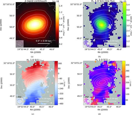
(a) the K-band continuum; (b): H2 1–0 S(1) integrated flux; (c): H2 1–0 S(1) radial velocity (minus the systemic velocity of the galaxy obtained from the redshift of z = 0.0602); and (d): H2 1–0 S(1) velocity dispersion (Gaussian σ). The K-band continuum is indicated in contours and the FWHM of the PSF (taking into account the effects of MAD smoothing) is indicated in all figures.
4.2.1 Kinematics
To determine whether the H2 belongs to the circumnuclear disc, we fit a simple disc model to our data using mpfit. Our model has solid-body rotation out to a break radius rb, and a flat rotation curve for r > rb, and we fit the systemic velocity as a free parameter. We do not account for beam smearing in the fit. Fig. 4 shows the model fit and residuals, and Fig. 5 shows a cross-section of the radial velocities taken along the dashed black line shown in Fig. 4. The disc fit has a PA approximately perpendicular to the jet axis, indeed consistent with that of the circumnuclear disc detected in previous studies. The fitted inclination of the disc is consistent with the easternmost edge being closest to us, which is also consistent with the greater H i opacity of the Eastern radio lobe (Conway 1996; Struve & Conway 2012). At the edge of the disc (|$r \approx 0.8\, \rm kpc$|), the rotational velocity |$v_c \approx 425\, \rm km\, s^{-1}$| with respect to the systemic velocity is comparable to that of the HCO+ emission (Ga07). Therefore, our disc fit shows the warm H2 probes the interior |${\sim } \rm kpc$| of the circumnuclear disc of 4C 31.04, where the apparent solid-body rotation is a result of the warm H2 not extending far enough into the disc to reach the turnover in the rotation curve.
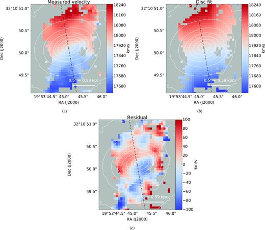
Kinematics of the H2 1–0 S(1) emission line; (a): measured radial velocity, (b) radial velocity of the model fit, and (c) the residual. With the exception of the residual plot, all velocities are given with respect to the local standard of rest. The cross represents the location of the nucleus (i.e. the peak in the K-band continuum). Fig. 5 shows a cross-section of the radial velocities taken along the dashed black line.
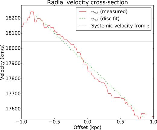
A cross-section of the measured (red solid line) and model fit (green dashed line) radial velocity taken along the black dashed lines indicated in Fig. 4. The systemic velocity of the galaxy, as estimated from the redshift, is indicated by the horizontal line, showing that the H2 emission has a systemic blueshift of |${\approx } 150\, \rm km\, s^{-1}$|.
Interestingly, the H2 emission has a net blueshifted velocity of |${\approx } 150\, \rm \, km\, s^{-1}$| relative to the systemic velocity derived using the redshift (z = 0.0602), which is markedly similar to that of HCO+ (Ga07) and H i (Struve & Conway 2012) viewed in absorption over the nucleus.
A uniform distribution of dust in the disc could cause the flux-weighted mean velocity to have a significant blueshift; however this scenario would require an unrealistically large AK. We instead speculate that the warm H2 traces clouds of gas being radially accelerated by jet plasma percolating through the disc, and that the net blueshift is because redshifted gas on the far side of the disc is obscured by extinction.
We note that the |${\sim }100\, \rm km\, s^{-1}$| uncertainty in the redshift could be the cause of this apparent blueshift. However, adopting a lower redshift to force the HCO+ , H i, and H2 components to coincide with the galaxy’s systemic velocity would result in the [Fe ii] emission in the nucleus being significantly redshifted. This would be difficult to explain under our interpretation that the [Fe ii] emission arises from the jet accelerating material out of the nucleus. We discuss this further in Section 5.3.3.
The velocity residuals of the disc fit (Fig. 4) reveal redshifted and blueshifted velocity residuals to the NE and SW of the nucleus, respectively, which are similar to the radial velocity of the [Fe ii] emission (Fig. 2c), suggesting the kinematics of the molecular disc could be disrupted by the same processes causing the [Fe ii] emission. However, referring to the HST R − H image (Fig. 1) and to the flux distribution of the warm H2 (Fig. 3b), the circumnuclear disc is clearly warped. The residuals in Fig. 4 could simply arise from our disc fit not accounting for this warp, and so this alone cannot be interpreted as evidence of kinematically disturbed molecular gas in the inner regions of the disc.
4.2.2 Gas temperature
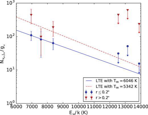
H2 excitation diagram of 4C 31.04. The red triangles and blue circles indicate estimates of Nobs(νu, Ju)/gu for the extended (r > 0.2 arcsec) and central (r ≤ 2 arcsec) regions, respectively. The arrows indicate emission lines for which we can only estimate upper limits.
The excitation diagram for the H2 1–0 S(1), S(2) and S(3) transitions in both the central and extended components of the H2 is shown in Fig. 6, where we plot Nobs(νu, Ju)/gu as a function of the temperature corresponding to the transition energy of each line. For non-detected emission lines we use the upper limits in these regions (Table 1). Unfortunately, due to the close spacing in temperature of the H2 1–0 S(1,2,3) transitions, and because we only have upper limits for the H2 2–1 S(1,2,3) lines, we cannot place a very restrictive constraint on the temperature in the extended component of the H2; however, the emission line fluxes in the central 0.4 arcsec are consistent with a temperature |$5000\!-\!6000\,\rm K$|, indicating that the H2 in the central regions is much hotter than the |${\sim } 300\, \rm K$| H2 probed by Spitzer observations (Willett et al. 2010).
4.2.3 Excitation mechanism
Ro-vibrational H2 emission can trace collisionally excited gas processed by shocks that are not fast enough to dissociate H2 molecules. These emission lines can also be emitted by H2 molecules excited by fluorescence from UV photons from O- and B-type stars. We use two key emission line ratios (Table 2) to demonstrate that shock excitation is the most likely scenario.
Ratios of the integrated fluxes of emission lines evaluated over the entire field of view (left column), within the central 0.2 arcsec (middle column) and outside the central 0.2 arcsec (right column). The integrated flux is measured by adding together the emission line fluxes in each individually fitted spaxel. The upper limits are computed using the method described in Section 3.
| Emission line ratio | Total | Within r ≤ 0.2 arcsec | Outside r > 0.2 arcsec |
|---|---|---|---|
| H2 1–0 S(1)/H i Br γ | 0.5774 | 1.5212 | 0.5000 |
| H2 1–0/2–1 S(1) | 0.8443 | 2.5826 | 0.7229 |
| Emission line ratio | Total | Within r ≤ 0.2 arcsec | Outside r > 0.2 arcsec |
|---|---|---|---|
| H2 1–0 S(1)/H i Br γ | 0.5774 | 1.5212 | 0.5000 |
| H2 1–0/2–1 S(1) | 0.8443 | 2.5826 | 0.7229 |
Shock-excited H2 can be distinguished from H2 excited by a UV stellar radiation field by the relative level populations: fluorescent excitation tends to populate higher level ν states more than shock excitation. Therefore, line ratios of ro-vibrational emission lines involving the same J state transition with different upper ν levels can be used as indicators of the excitation mechanism. In shock-heated gas, the ratio of the H2 1–0/2–1 S(1) lines tends to be much larger than in fluorescently excited gas (e.g. Nesvadba et al. 2011). Fig. 7a shows this ratio in each spaxel. We have used upper limits to estimate the 2–1 S(1) flux; therefore these values should be interpreted as lower limits for the true line ratio. In the inner 0.4 arcsec, the ratio of the integrated fluxes of the two lines exceeds ∼2, indicating shock excitation.
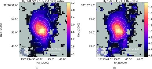
Emission line ratio maps that we use to determine the excitation mechanism for the warm H2 in different regions. (a) shows the H2 1–0 S(1)/H2 2–1 S(1) ratio and (b) shows the H2 1–0 S(1)/Br γ ratio, and the white contours show the H2 1–0 S(1) flux. The values of ∼3 and ∼2 in the inner 0.4 arcsec in (a) and (b), respectively, suggest shocks, and not SF, are the likely excitation mechanism.
At high enough densities (n ≳ 103 cm−3), where H2 is in LTE, level populations will be similar in both shock- and fluorescent-excited H2, in which case the line ratios are misleading. Here, we can eliminate fluorescent excitation by young stars because we do not detect Br γ, leaving shocks as the most likely mechanism. Fig. 7b shows the ratio H2 1–0 S(1)/Br γ in each spaxel, where we have used upper limits to estimate the Br γ flux. In the inner 0.4 arcsec, the ratio of the integrated fluxes of the two lines exceeds the 0.1–1.5 expected when the excitation source is UV heating in star-forming galaxies (Puxley, Hawarden & Mountain 1990). Additionally, our Br γ upper limits are pessimistic, because we assume a Gaussian sigma determined from the combined H α + [N ii] equivalent width of Marcha et al. (1996) from an unresolved spectrum. Therefore, combining this result with the high H2 1–0/2–1 S(1) ratio, we conclude that the ro-vibrational H2 emission is excited by shocks in the central region.
In the extended component, we cannot rule out SF as the source of excitation, although we note these results are not inconsistent with shock excitation, because both line ratios involve upper limits.
4.2.4 Mass estimates
We now estimate the dynamical mass and warm gas mass and compare our results with those from previous studies in Section 2.3.
Solid-body rotation in the H2 radial velocity implies the mass distribution interior to the disc can be approximated as a uniform-density sphere. We estimate the enclosed dynamical mass using Mdyn = vc(r)2r/G where vc(r) ∝ r is the rotational velocity at radius r and G is the gravitational constant. From our best-fitting thin-disc model, the rotational speed of the disc at its edge is |$v_c(r = 0.8 \text{\,kpc}) \approx 425$| km s−1 and a dynamical mass |$M_\text{dyn} \approx 3.4 \times 10^{10}\, \rm M_\odot$|.
Willett et al. (2010) also estimate the mass of warm H2 using mid-IR pure rotational (0–0) H2 emission lines from Spitzer observations. For 4C 31.04 they find |$M_{\text{${\rm H}_{2}$,\rm warm}} = (4.7 \pm 1.3) \times 10^{6}\, \rm M_\odot$| at a temperature |$T = 338 \pm 100\,\rm K$|, a mass ∼102 greater than the mass of much warmer H2 we find. Combined with the temperature constraints provided by our excitation diagram (Fig. 6), we conclude that the ro-vibrational emission we detect in our NIFS observations traces a small, and relatively hot, fraction of the total warm H2 in the nucleus of 4C 31.04.
In Table 3, we compare the mass estimates of different ISM phases of 4C 31.04 from this work and the literature. We assume that the most reliable estimate of the cold H2 gas mass is that of Ocaña Flaquer et al. (2010) derived from CO measurements, which gives a warm H2-to-total molecular gas mass fraction of ∼10−3.
Mass estimates of different gas phases in 4C 31.04.
| Phase | Mass |$(\rm M_\odot)$| | Reference |
|---|---|---|
| MBH | ≤108.16 | Willett et al. (2010) |
| |$M_\text{dyn} (r \lt 0.8\, \rm kpc)$| | 3.4 × 10¹⁰ | This work |
| |$M_{\text{${\rm H}_{2}$,\rm warm}}\, (\rm T = 2000\, \rm K)$| | 9.7 × 10³ | This work |
| |$M_{\text{${\rm H}_{2}$,\rm warm}}\, (\rm T = 338 \pm 100\rm K)$| | (4.7 ± 1.3) × 106 | Willett et al. (2010) |
| |$M_{\text{${\rm H}_{2}$}, \rm cold}$| | (60.63 ± 16.92) × 108 | Ocaña Flaquer et al. (2010) |
| |$M_\rm{H\,\small {I}{}}$| | 4.8 × 10⁷ | Perlman et al. (2001) |
| |$N_\rm{H\,\small {I}{}}$| | |$(1.2-2.4) \times 10^{21}\, \rm \, cm^{-2}$| | Struve & Conway (2012) |
5 DISCUSSION
In this section, we analyse the energetics, kinematics, and morphology of the [Fe ii] and H2 emission and argue that they indicate strong jet-ISM interactions are occurring in 4C 31.04.
Hydrodynamical simulations have shown that young, compact jets such as those in 4C 31.04 are capable of influencing the evolution of their host galaxies by injecting turbulence and driving shocks into the ISM (e.g. Sutherland & Bicknell 2007; Wagner & Bicknell 2011; Mukherjee et al. 2016, 2018a, b). Importantly, the coupling efficiency of the kinetic energy and momentum from the jet into the ISM peaks in these early stages of jet evolution (Wagner & Bicknell 2011; Mukherjee et al. 2016), emphasizing the importance of this epoch in the context of jet-driven feedback.
In an early phase of jet evolution described as the ‘energy-driven bubble’ stage by SB07, the jets become deflected and split as they encounter dense clumps in the ISM, forming streams of plasma that percolate through the ISM over a broad solid angle. Mid-plane density and temperature slices of a hydrodynamical simulation showing this phenomenon are shown in Fig. 8, with corresponding synthetic radio images shown in Fig. 9. The jet plasma inflates a high pressure, pseudo-spherical, energy-driven bubble that drives a forward shock into the ISM, dispersing clouds and accelerating them outwards. The low-density synchrotron-emitting plasma in the bubble cavity manifests as extended, low surface brightness radio emission (e.g. fig. 5 in Wagner & Bicknell 2011). Simulations of jets propagating into dense, clumpy discs (Mukherjee et al. 2018a) have shown that jets may also drive subrelativistic flows of plasma into the disc plane, inducing shocks and turbulence. The jet plasma ablates clouds, and triggers hydrodynamical instabilities that form filaments. Ram pressure and thermal pressure gradients from shocks accelerates these clouds and filaments in a radial direction, introducing significant non-circular motions into the disc.
![Mid-plane slices from a hydrodynamical simulation of a jet with $F_{\rm jet} = 10^{45}\, \rm erg\, s^{-1}$ propagating in the Z-direction through a clumpy disc at an angle of 20° [model C of Mukherjee et al. (2018a); see their table 2 for simulation parameters]; (a) shows the density and (b) shows the temperature. The magenta contours represent jet plasma that will emit brightly in the radio (jet tracer value ϕ = 0.5) and the black contours trace much fainter plasma (ϕ = 0.005) which fills the jet-driven bubble and drives shocks into the surrounding ISM.](https://oup.silverchair-cdn.com/oup/backfile/Content_public/Journal/mnras/484/3/10.1093_mnras_stz233/1/m_stz233fig8.jpeg?Expires=1750562609&Signature=fVLhk9KafvwF2OoyTrV2ffcXT0szXtle~uh4W6sG1I7PoEssEf5W9e7kd3cQFq32oi2zumkzNAUYkQHJKOkwzGAqKZS7gWDIT6VnSmXnXZtEmkOJ8NACiM0Q9D5IUG7aGYdUA5aNk9BL2ZlrX8DDxWh8-flquTWqIjcm5OJvwMmi1ptXy5kNRKdEqI6RY-mdH0zIKIe2GdTwMK887k2W10Mya~GFT0759GDAKhOwOr4uEnVkT2s8f5JO-GrvE7fw2O1S49TBUFCOmstQ~rRctWalbkGe0fxZIEegPbPnhWKn3usB2TuYFRAT9hqZIX1AUVd1y~iEMAJk0sVCLyVOaA__&Key-Pair-Id=APKAIE5G5CRDK6RD3PGA)
Mid-plane slices from a hydrodynamical simulation of a jet with |$F_{\rm jet} = 10^{45}\, \rm erg\, s^{-1}$| propagating in the Z-direction through a clumpy disc at an angle of 20° [model C of Mukherjee et al. (2018a); see their table 2 for simulation parameters]; (a) shows the density and (b) shows the temperature. The magenta contours represent jet plasma that will emit brightly in the radio (jet tracer value ϕ = 0.5) and the black contours trace much fainter plasma (ϕ = 0.005) which fills the jet-driven bubble and drives shocks into the surrounding ISM.
![Synthetic radio surface brightness maps corresponding to the simulated mid-plane density and temperature slices shown in Fig. 8 at rest-frame 5 GHz with dynamic ranges of 106 and 102, respectively. The axis labels are in kpc and the intensity is given in $\log \left[P (\rm W\, Hz^{-1}\, kpc^{-2}\, Sr^{-1})\right]$. Comparing (a) and (b) demonstrates that a high dynamic range may be necessary to observe low surface brightness plasma extending beyond the radio lobes into the jet-driven bubble. We note that the dynamic range of (b) is comparable to that of the 5 GHz VLBI observations of 4C 31.04 by Gi03, suggesting that higher dynamic range observations could reveal jet plasma out to the extent of the [Fe ii] emission we observe in 4C 31.04.](https://oup.silverchair-cdn.com/oup/backfile/Content_public/Journal/mnras/484/3/10.1093_mnras_stz233/1/m_stz233fig9.jpeg?Expires=1750562609&Signature=e4apUN~nqbMYXBUH1zTwS6vN-lLpoxLfM0k3jo~Gu~WdY5BBRhQ9KW8-BqodrmsWfR6Os4UdsKa~X3TMxDDdbr7S4TloYnTFaS52NVZ9iBAvpCq9jDW3MddxTXnWRTwptJf~MRGOFLhzIytuqylDVGoPbysQUUgO0G3FRmdfwBiHstGtn3QnYunFzCF8~xDkiFrrWTJWfYO~tKsikel3GqN3xsrszAz~r26sX38Qy-7BFOOuQwXCoepPYzKvxLH7w78hh4ZQJVr25I~ehEMJSs103640fpxf0AzxFD8V2eBEeU0VKofFe8Tvp1QFgaf-8F8Ctp9Bqg6RmwCH-kQ7Dg__&Key-Pair-Id=APKAIE5G5CRDK6RD3PGA)
Synthetic radio surface brightness maps corresponding to the simulated mid-plane density and temperature slices shown in Fig. 8 at rest-frame 5 GHz with dynamic ranges of 106 and 102, respectively. The axis labels are in kpc and the intensity is given in |$\log \left[P (\rm W\, Hz^{-1}\, kpc^{-2}\, Sr^{-1})\right]$|. Comparing (a) and (b) demonstrates that a high dynamic range may be necessary to observe low surface brightness plasma extending beyond the radio lobes into the jet-driven bubble. We note that the dynamic range of (b) is comparable to that of the 5 GHz VLBI observations of 4C 31.04 by Gi03, suggesting that higher dynamic range observations could reveal jet plasma out to the extent of the [Fe ii] emission we observe in 4C 31.04.
Our observations, together with its young age and small size, strongly suggest that the radio jets of 4C 31.04 are in the ‘energy-driven bubble’ stage, where the jets are interacting strongly with the dense and clumpy circumnuclear disc. By comparing our observations with hydrodynamical simulations, we formulate the model described by Fig. 10, which shows a top-down cross-sectional view of the circumnuclear disc of dust and atomic and molecular gas orbiting the nucleus. The inclination of the disc is such that the Eastern radio lobe is obscured; this is consistent with the greater H i opacity on that side (Conway 1996; Struve & Conway 2012). The 100 pc-scale radio lobes (dark green) are shown to scale. The jet plasma inflates an expanding bubble which drives fast shocks into the surrounding ISM, destroying dust grains and launching material out of the disc plane, which is traced by [Fe ii] (dark red) and high-velocity H i clouds (pale blue circles) detected in absorption by Conway (1996). Shocked ionized gas (transparent circles) free–free absorbs synchrotron emission from the jet plasma, causing the spectral turnover at 400 MHz. The jet plasma also drives radial flows into the disc, decelerating as it shocks molecular gas (blue), causing ro-vibrational H2 emission. The plasma may also radially accelerate this gas to speeds |${\sim } 100\, \rm km\, s^{-1}$|, giving rise to non-circular motions including blueshifted H2 emission and HCO+ and H i absorption.
![A top-down cross-section view of 4C 31.04 showing different components of the shocked gas in context, approximately to scale. Indicated in dark green are the 100 pc-scale radio lobes visible in VLBI observations (Giovannini et al. 2001; Giroletti et al. 2003). The paler green region represents low surface brightness jet plasma filling the jet-driven bubble, which drives a shock into the surrounding gas and causes [Fe ii] emission (dark red). Jet plasma also percolates radially through channels in the clumpy circumnuclear disc (blue), driving shocks into neutral gas and causing H2 emission. Clouds of ionized gas that free–free absorb synchrotron radiation from the jet plasma cause the spectral turnover at 400 MHz are indicated in transparent circles. The pale blue circles represent clouds of neutral gas. The line of sight is indicated by the dashed line; the disc is inclined such that the Western lobe is partially obscured by the disc, whereas the Eastern lobe is completely obscured by the disc, which is consistent with the H i absorption map (Conway 1996; Struve & Conway 2012).](https://oup.silverchair-cdn.com/oup/backfile/Content_public/Journal/mnras/484/3/10.1093_mnras_stz233/1/m_stz233fig10.jpeg?Expires=1750562609&Signature=Vr~cDXHImQv5D5xhwBLQlWdnqupc4wORPUcB5gI39tw0o4oy5JfY24~tZ4tiE0GvdzL06UXbjMgrsY6j-IT7GvNWN1i9LxDT3hS2CUB1DrN09Hh1fhqkngSAclIKzfXC8LlHvLAgGeFGAfS~bWqg6jeYRRqZ5GhYSQWyIH5YxkJ3mU4K-xly8Hnz~hZw7nwr9oq0DXz7N-tkQ7idMzEBJgeHOrmJh1KgdghDV2J9d9QyIlEHieNeVa0fPSgZgc0AG7AZ2AGSJGho1vfUaPXDzOMc480BqzX-LKES-H-AWO~Spivuj8Lb0ms6kco7KIPKrM0ey6dUpD1s8ENN2vJmaw__&Key-Pair-Id=APKAIE5G5CRDK6RD3PGA)
A top-down cross-section view of 4C 31.04 showing different components of the shocked gas in context, approximately to scale. Indicated in dark green are the 100 pc-scale radio lobes visible in VLBI observations (Giovannini et al. 2001; Giroletti et al. 2003). The paler green region represents low surface brightness jet plasma filling the jet-driven bubble, which drives a shock into the surrounding gas and causes [Fe ii] emission (dark red). Jet plasma also percolates radially through channels in the clumpy circumnuclear disc (blue), driving shocks into neutral gas and causing H2 emission. Clouds of ionized gas that free–free absorb synchrotron radiation from the jet plasma cause the spectral turnover at 400 MHz are indicated in transparent circles. The pale blue circles represent clouds of neutral gas. The line of sight is indicated by the dashed line; the disc is inclined such that the Western lobe is partially obscured by the disc, whereas the Eastern lobe is completely obscured by the disc, which is consistent with the H i absorption map (Conway 1996; Struve & Conway 2012).
5.1 Updated jet flux estimate
Comparing the jet flux with observed emission line luminosities is important in determining whether it is plausible for the jets to be causing the line emission. Hence, before we discuss the excitation mechanisms for the [Fe ii] and H2 emission in Sections 5.2 and 5.3, respectively, we provide an updated estimate of the jet flux of 4C 31.04.
Parameters used in determining the jet flux. Output parameters are denoted with daggers (†).
| Parameter | Symbol | Value |
|---|---|---|
| Min. electron Lorentz factor | γ1 | 102 |
| Max. electron Lorentz factor | γ2 | 105 |
| Age of radio lobes (Gi03) | tlobe | |$5000\, \rm yr$| |
| Temperature of ambient ISM | Ta | |$10^7\, \rm K$| |
| Density of ambient ISM | na | |$0.1\, \rm cm^{-3}$| |
| Radius of jet-blown bubble | |$R_{\rm [Fe\,\small{II}]}$| | |$175\, \rm pc$| |
| Eastern jet flux† | |$F_{\rm jet,\, Eastern\, lobe}$| | |$1.50 \times 10^{44}\, \rm erg\, s^{-1}$| |
| Western jet flux† | |$F_{\rm jet,\, Western\, lobe}$| | |$1.44 \times 10^{44}\, \rm erg\, s^{-1}$| |
| Total jet flux | Fjet | |$2.94 \times 10^{44}\, \rm erg \,s^{-1}$| |
5.2 The origin of the [Fe ii] emission
Fast shocks destroy dust grains, releasing Fe i into the gas phase, which then becomes singly ionized by the interstellar radiation field. In the post-shock region, Fe ii becomes collisionally excited and emits emission lines in the near-IR, including [Fe ii], which can therefore be used as a shock tracer.
Fig. 2 shows that the [Fe ii] emission is localized to the innermost few 100 pc of the nucleus, and that the radial velocity field is consistent with material being ejected from the disc plane on either side. The kinematics and location of the [Fe ii] emission suggest that it arises from shocks driven by the expanding bubble inflated by the radio jets.
We now use the measured SFR to estimate νSNrate using a solar metallicity Starburst99 (Leitherer et al. 1999) model with a continuous |$1\, \rm \rm M_\odot \, \rm yr^{-1}$| SF law and a Salpeter IMF at an age of |$1\, \rm Gyr$|. After multiplying to match the SFR of 4C 31.04 (|$4.9\, \rm M_\odot \,\rm yr^{-1}$|, Ocaña Flaquer et al. 2010) we find |$\nu _{\text{SNrate, SFR}} = 0.1 \rm yr^{-1}$|, less than half the rate required to power the [Fe ii] emission.
We therefore rule out SF as the excitation mechanism for the [Fe ii], and instead argue that the emission is driven by a jet-ISM interaction. As illustrated in Fig. 10, the bubble drives fast shocks into the ISM, destroying molecular gas. The shocked gas is accelerated outwards by the forward shock and also by the jet streams, creating an expanding bubble illuminated in [Fe ii].
5.3 The origin of the H2 emission
Large masses of warm H2 seem to be common in the hosts of nearby radio galaxies, suggesting a link between the H2 emission and radio activity (e.g. Nesvadba et al. 2010; Ogle et al. 2010). As discussed in Section 4.2, we detect ro-vibrational H2 emission in the circumnuclear disc |${\approx } 2\, \rm kpc$| in diameter, which probes relatively hot (|${\sim } 10^3\, \rm K$|) molecular gas. The line ratios show the warm H2 is shock excited (Table 2 and Fig. 7).
In this section, we show that the |${\sim } 10^3\rm\, K$| H2 represents a relatively hot fraction of a much larger reservoir of H2 heated by a jet-ISM interaction, the bulk of which is much cooler (|${\sim } 10^2\, \rm K$|). In our model, shown in Fig. 10, the jet-driven bubble drives fast shocks into the gas at small radii, causing [Fe ii] emission, before decelerating as it drives shocks into the denser molecular gas in the disc. We also postulate that jet plasma percolating radially throughout the disc also accelerates clouds to the observed systemic blueshift of |${\approx } 150\,\rm km\, s^{-1}$| in the warmer H2 component (Fig. 3c).
5.3.1 Excitation mechanism
The ro-vibrational-emitting H2 probed by our observations is very warm (Fig. 6), and cools rapidly. This phase is therefore very short-lived, and accordingly only represents a very small fraction of the total H2 mass (Table 3). Willett et al. (2010) report a much larger (|${\sim } 10^6 \,\rm M_\odot$|) reservoir of cooler H2, at a temperature |${\sim } 300 \,\rm K$|. We wish to determine whether this cooler component represents gas in the circumnuclear disc that has been processed by the jets and since cooled; to do this we use mid-IR diagnostics to reveal the excitation mechanism of the cooler H2 component.
Using the combined luminosity of the H2 0–0 S(0, 1, 2, 3) lines (Willett et al. 2010) we place a lower limit on the ratio |$L(\rm {H_2}) / L(\rm {PAH\, 7.7\, \mu m}) \ge 0.1$|, where we calculate the luminosity of the PAH feature at |$7.7\, \mu \rm m$| using that of the |$11.3\, \mu \rm m$| and assuming |$L(\rm {PAH\, 6.2\, \mu m})/L(\rm {PAH\, 7.7\, \mu m}) = 0.26$|, which holds for the sample of H2-luminous radio galaxies of Ogle et al. (2010); this gives |$L(\rm PAH,\, 7.7) = 1.55 \times 10^{42}\, \rm erg\, s^{-1}$|. The criterion of Ogle et al. (2010) (|$L(\rm {H_2}) / L(\rm {PAH\, 7.7\, \mu m}) \gt 0.04$|) strongly suggests the H2 is shock heated.
We also use the diagnostic diagram of Nesvadba et al. (2010, their fig. 6), which separates SF from other mechanisms as the source of H2 heating using the luminosity ratios of the summed H2 0–0 S(0)–S(3) lines to the |$^{12}\rm CO(1-0)$| and to the PAH feature at |$7.7\, \rm \mu m$|. While the CO emission traces cold molecular gas from which stars form, PAH features trace UV photons excited by SF; hence these ratios can be used to indicate the contribution of SF in photon-dominated regions (PDRs) to the H2 heating. To calculate the CO(1 − 0) luminosity, we convert the ICO given by Ocaña Flaquer et al. (2010) into a luminosity using equation (3) of Solomon et al. (1997), yielding |$L(\rm CO) = 3.56 \times 10^{38}\, \rm erg\, s^{-1}$|. We find |$L(\rm H_2) / L(\rm PAH,\, 7.7) \ge 0.148$| and |$L(\rm H_2) / L(\rm CO) \ge 6.43 \times 10^{2}$|, placing 4C 31.04 well outside the regions covered by PDR models, showing that the |${\sim } 300\, \rm K$| H2 component is not predominantly heated by UV photons, leaving shocks, cosmic rays, and X-ray heating as plausible mechanisms.
Based on our above arguments, both the |${\sim } 100\, \rm K$| and |${\sim } 10^3\, \rm K$| H2 is heated by a mechanism other than SF. We argue that the |${\sim } 10^3\, \rm K$| and |${\sim } 100 \,\rm K$| H2 are physically associated; in this case the strong shock signature we observe in the former (Fig. 7) shows that the warm H2 is shock excited.
5.3.2 What is driving the shocks?
To obtain Φ(r) and vc(r), we fit a simple 1/n Sersić profile to the K-band continuum and use the analytical expressions given by Terzić & Graham (2005). We estimate the stellar mass M* from the 2MASS Ks-band magnitude using a simple stellar population model of Bruzual & Charlot (2003) with a single instantaneous burst of SF, assuming solar metallicity, a Chabrier IMF, and an age of a few Gyr. This yields log M* ≈ 11.4. To check the validity of our M* estimate, we compare the circular velocity predicted by the model with that of the warm H2 in the circumnuclear disc from our NIFS observations. We find that a lower stellar mass log M* = 10.9 is better able to reproduce the observed vc at |$1\, \rm kpc$|. However, we find that this correction only changes the resulting accretion disc luminosity to within an order of magnitude; hence, for simplicity, we use the stellar mass predicted by the 2MASS Ks-band magnitude.
If we assume a steady-state accretion model, that is |$\dot{M}$| is equal to the accretion rate on to the black hole, and that |$10{{\ \rm per\ cent}}$| of the rest-mass energy of the accreted material per unit time is emitted in the form of the radio jets, i.e. |$L_{\rm BH} = 0.1 \dot{M} c^2 = 2.94 \times 10^{44}\, \rm erg\, s^{-1}$|, then the accretion rate |$\dot{M} \approx 0.05\, \rm M_\odot \, \rm yr^{-1}$|. Using equation (8), we estimate an accretion disc luminosity |$L_{\rm disc} \sim 10^{40}\, \rm erg\, s^{-1}$|, an order of magnitude lower than the observed H2 0–0 luminosity |$L_{\text{${\rm H}_{2}$}} \ge 2.3\times 10^{41} \rm \, erg\, s^{-1}$|, enabling us to rule out accretion as the mechanism heating the H2. Meanwhile, the H2 luminosity represents |${\sim } 0.1{{\ \rm per\ cent}}$| of the estimated jet flux (Section 5.1), so that there is ample jet power to drive the H2 luminosity via radiative shocks. We therefore conclude that the shocks are being driven by the jets, a scenario which also explains the sharp peak in the H2 flux in the vicinity of the nucleus (Fig. 3b).
5.3.3 Explaining the peculiar blueshift in the H2
Shocks induced by a jet-ISM interaction out to kpc-scale radii in the circumnuclear disc could explain the peculiar systemic blueshift of |${\approx } 150\, \rm km\, s^{-1}$| we observe in the H2 (Fig. 3c) relative to the redshift z = 0.0602 of Ga07.
Previous observations have revealed cold gas components with remarkably similar blueshifts: Ga07 detected an unresolved HCO+ component in absorption over the nucleus with a systemic blueshift of |${\approx } 150\, \rm km\, s^{-1}$|, while Struve & Conway (2012) found that the centre of the integrated H i absorption profile is centred on a similar blueshifted systemic velocity. The absorption profile also has a blue wing (their fig. 7) extending to |${\sim } 200\, \rm km\, s^{-1}$|. Prominent blue wings in the H i absorption profiles of powerful radio galaxies are a signature of fast neutral outflows (Morganti et al. 2005); we speculate that the blue wing in the profile of 4C 31.04 indicates that the jets are accelerating neutral gas out of the nucleus, albeit to much lower velocities than are observed in these more extended radio galaxies.
It is possible that the redshift is in fact lower than the estimate of Ga07, and that the H2 rotation curve is centred on the systemic velocity of the galaxy. Ga07 calculated the redshift of 4C 31.04 by assuming that the HCO+ emission components to the north and south of the nucleus represented gas rotating in the disc, and that the mean velocity of the two components corresponds to the galaxy’s systemic velocity. Struve & Conway (2012) argue that this assumption may be flawed if gas in the disc is dynamically unsettled. Correcting the redshift to remove the blueshift in the |${\sim } 10^3\, \rm K$| H2, H i, and HCO+ absorption yields z = 0.0597 ± 0.001. While this is consistent with the redshift from optical spectroscopy [z = 0.060 ± 0.001, Marcha et al. (1996)], it would mean the [Fe ii] emission is in fact redshifted by |${\approx } 150\,\rm km\, s^{-1}$|, which would be difficult to explain under our interpretation that it traces a jet-driven bubble.
An alternate explanation is that the blueshifted warm and cold molecular phases trace clouds of gas being radially accelerated in circumnuclear disc by jet plasma. As mentioned earlier, hydrodynamical simulations by Mukherjee et al. (2018a) of jets evolving in galaxies with clumpy gas discs have shown that the expanding bubble driven by the jets drives subrelativistic radial flows into the disc plane. These flows drive turbulence and shocks into the gas, and introduce significant non-circular motions. In addition to the observed blueshifted gas, radial flows of jet plasma may be able to explain the reported unrelaxed dynamics in the gas disc (Pe01, Ga07), which has previously been attributed to gas settling on to the disc in the process of accretion. We note that |${\sim } 100\, \rm pc$|-scale equatorial outflows have been recorded in other radio galaxies, such as NGC 5929 (Riffel, Storchi-Bergmann & Riffel 2015) and NGC 1386 (Lena et al. 2015). These outflows have tentatively been attributed to torus outflows or accretion disc winds; it is unclear whether this mechanism could drive the relatively low-velocity blueshifted gas we observe in 4C 31.04.
We now calculate the kinetic energy associated with the observed blueshift in the H2 to show that it is plausible that it is driven by the jets. Assuming that both the |${\sim } 100\rm\, K$| and |${\sim } 10^3\rm\, K$| H2 are accelerated to the observed blueshifted velocity, the cooler component (|$4.7 \pm 1.3 \times 10^{6}\, \rm \rm M_\odot$|, Willett et al. 2010) will dominate the kinetic energy. If the blueshifted clouds have a velocity |$150\, \rm km\, s^{-1}$|, then the associated kinetic energy is |${\approx } 1.1 \times 10^{54}\, \rm erg$|. Assuming the gas is being pushed radially outwards at a constant velocity, the time taken for material to reach the farthest extent of the warm H2 disc |${\approx } 1\, \rm kpc$| from the nucleus is |$\tau = 6.5 \times 10^6\, \rm yr$|. Assuming the jet has been accelerating this gas over this time period, this yields an energy injection rate |${\sim } 10^{41}\, \rm erg\, s^{-1}$|, approximately |$0.1{{\ \rm per\ cent}}$| of the jet power we estimated in Section 5.1, showing that it is indeed plausible.
In light of these arguments, we tentatively agree with the redshift quoted by Ga07, and speculate that the blueshifted H2, H i, and HCO+ traces gas clouds being radially accelerated in the disc plane by the jet plasma. Confirmation of this scenario will require further observations, e.g. high-resolution optical spectroscopy to measure the galaxy’s redshift using stellar absorption features.
5.3.4 How far does the jet plasma extend?
In the previous sections we have shown that both the [Fe ii] and H2 emission are caused by a jet-ISM interaction. However, the radio lobes extend |${\approx } 60\rm \, pc$| from the nucleus, whereas we detect [Fe ii] over a region ≈three times larger, and warm H2 out to |${\sim } \rm kpc$| radii–how could this emission possibly arise from a jet-ISM interaction?
Hydrodynamical simulations of jets propagating into clumpy discs (Mukherjee et al. 2018a) show that the brightest regions of jet plasma may become temporarily frustrated by dense clouds in the disc, slowing its propagation. This effect becomes more pronounced when the jets are inclined with respect to the disc normal, as it increases the effective path-length over which the jets interact with the dense ISM. Meanwhile, the expanding bubble can advance rapidly once it escapes the dense ISM in the disc plane, allowing the bubble radius to grow several times larger than the radio lobes.
Our observations show the jets in 4C 31.04 are likely to be inclined ∼10°−20° to the normal of the circumnuclear disc. This geometry is supported by the inclination of ∼60° we measure from the warm H2 and by the jets being at an angle of ≲ 15° with respect to the sky, with the Western lobe nearest (Giovannini et al. 2001). Moreover, the kinematics of the [Fe ii] emission line (Fig. 2c) shows material being accelerated off the disc plane such that the Western lobe is pointing towards us.
In order to illustrate the role that a dense and clumpy disc can play in determining the outcome of a jet-ISM interaction, we show mid-plane density and temperature slices from a hydrodynamical simulation in which the jets are inclined 20° to the disc normal in Fig. 8. In Fig. 8a, the brightest parts of the jet plasma (magenta contours), particularly in the +ve Z-direction, have become halted at short distance from the nucleus. Meanwhile, lower surface brightness plasma (black contours) propagates along channels in the clumpy ISM and fills the much larger bubble, which crucially may go undetected in high-resolution VLBI observations despite interacting strongly with the surrounding ISM. In Figs 9a and b, we show corresponding synthetic 1 GHz surface brightness maps with high and low dynamic ranges, respectively, where we define the dynamic range as the maximum measured flux divided by the minimum flux level that can be detected. Comparing the two illustrates the importance of a high dynamic range in revealing the low surface brightness plasma that traces the true extent of the jet-driven bubble. We note that Fig. 9b is missing only |${\approx }1{{\ \rm per\ cent}}$| of the total flux recovered in Fig. 9a. This illustrates that VLBI observations with flux completeness measurements in excess of |$99{{\ \rm per\ cent}}$| can miss jet plasma that may still be interacting strongly with the surrounding ISM.
Multiple flux completeness measurements of VLBI observations of 4C 31.04 indeed indicates that some large-scale structure exists at lower surface brightnesses than have been observed. Cotton et al. (1995) find that 98 per cent and 76 per cent of the flux density of 4C 31.04 measured with the VLA is recovered in VLBI observations at 1.7 and 8.4 GHz, respectively. Gi03 find that approximately 90 per cent of the flux measured with single-dish observations is recovered with VLBI at 5 GHz. Altschuler et al. (1995) recover 80 per cent of the total flux density at 92 cm. We note that the 5 GHz VLBI image of Gi03 has a dynamic range of ∼100; this, combined with the |${\sim } 75\!-\!95{{\ \rm per\ cent}}$| flux completeness of GHz-range VLBI observations, suggests that 4C 31.04 may indeed harbour low surface brightness radio emission out to the radii at which we observe shocked gas, resolving the inconsistency between the extent of the shocked gas and the radio lobes.
5.4 Age of the radio source
We cannot estimate the true age of the radio jets in 4C 31.04 with existing VLBI observations as they resolve out low surface brightness radio emission that fills a much larger bubble revealed by our NIFS observations. Moreover, because the rate at which synchrotron-emitting electrons lose energy E is proportional to E2, high-frequency, high surface brightness radio emission only probes the youngest synchrotron electrons; parts, or even most, of the emission from the jet plasma may be missed by GHz-frequency observations with a small dynamic range. We instead use the jet flux and our NIFS observations to estimate the true age of the radio jets.
We calculate a lower limit for the age of the radio source by assuming that the jet plasma has only reached the extent of the [Fe ii] emission, ignoring the extended H2 emission. In this case, we set |$R_\mathrm{ b} \approx 175\, \rm pc$| and find |$t_\mathrm{ b} \approx 17\, \rm kyr$|, more than three times older than the age estimated using synchrotron spectral decay (4000–5000 yr, Gi03).
In Section 5.3.2, we estimated an upper limit for the jet age |$6.5 \times 10^6\, \rm yr$| by calculating the time taken for material to reach the farthest extent of the warm H2 disc, and is an upper limit as the gas may have decelerated along its trajectory.
Although these age estimates are very crude, together they suggest that the previous age estimates based on VLBI imaging alone may not represent the true age of the source. Our results demonstrate the importance of optical or near-IR tracers of jet-ISM interaction in estimating the true extent of the jet plasma, particularly when existing radio observations have a low dynamic range or are not sensitive to the angular scales associated with the diffuse plasma filling the jet-driven bubbles.
5.5 Density distribution of the clumpy ISM
Free-free absorption (FFA) by clumpy gas ionized by the radio jets is a feasible cause of the spectral turnover in GPS and CSS sources (Bicknell et al. 2018). Here, we use the peak in the radio spectrum of 4C 31.04 to infer the parameters of the density distribution of the ionized, free–free absorbing ISM, in order to inform future hydrodynamical simulations. We use a simple analytical model to calculate the specific intensity of synchrotron-emitting plasma embedded in a clumpy free–free absorbing medium.
We calculate μ and σ2 as follows, using the input parameters shown in Table 5. First, we use a MAPPINGS V (Sutherland et al. 2013) model grid with non-equilibrium cooling and solar abundances to compute the fractional abundances of electrons, H+, He+, and He++ at a temperature |$T \approx 10^4\, \rm K$|. For each species, we use these values to calculate χν, i (Z) using equation (16). Then, by setting τν = 1 at the spectral peak (|$400\, \rm MHz$|) in equation (17), we solve for E(n2). We then find s using equation (18), which in turn allows us to find m using using equation (12). Finally, we solve for μ and σ using equations (11) and (13), yielding |$\mu = 15.5\, \rm cm^{-3}$| and |$\sigma ^2 = 1.86 \times 10^{4}\, \rm cm^{-6}$|.
Parameters used in determining the parameters of the lognormal density distribution. Output parameters are denoted with daggers (†).
| Parameter | Symbol | Value |
|---|---|---|
| Peak frequency | νpeak | |$400\, \rm MHz$| |
| Depth of absorbing slab | L | |$100\, \rm pc$| |
| Temperature | T | |$10059\, \rm K$| |
| Mean molecular mass | μ′ | 0.66504 |
| Electron fractional abundance | ne/n | 0.47175 |
| H+ fractional abundance | |$n_{\rm H^+} / n$| | 0.41932 |
| He+ fractional abundance | |$n_{\rm He^+} / n$| | 0.024458 |
| He++ fractional abundance | |$n_{\rm He^{++}} / n$| | 0.013770 |
| Velocity dispersion | σv | |$350\, \rm km\, s^{-1}$| |
| Turbulent forcing parameter | b | 0.4 |
| Ratio of thermal to magnetic pressure | β | 1 (equipartition) |
| Expected value of n2 † | E(n2) | |$1.89 \times 10^{4}\, \rm cm^{-6}$| |
| Mean density† | μ | |$15.5\, \rm cm^{-3}$| |
| Density variance† | σ2 | |$1.86 \times 10^{4}\, \rm cm^{-6}$| |
6 CONCLUSION
We have reported H- and K-band Gemini/NIFS observations of the CSS source 4C 31.04, a young AGN with jets interacting strongly with a clumpy ISM. The host of 4C 31.04 is a z = 0.0602 elliptical galaxy that harbours |${\sim } 10^{9}\rm \, \rm M_\odot$| of gas in a circumnuclear disc |${\approx } 2\rm \, kpc$| in diameter.
In the central few |$100\rm \, pc$|, we detect [Fe ii] emission that has a radial velocity field consistent with an expanding bubble driven by the jets. We rule out SNe explosions as the cause of the [Fe ii] emission; moreover, the kinematics of the line trace an expanding bubble, implying the emission is a result of a jet-ISM interaction.
We also detect ro-vibrational H2 emission that traces |${\sim } 10^4\, \rm M_\odot$| of very warm (|${\sim } 10^3\, \rm K$|) H2. This warm molecular phase traces rapidly cooling gas in the innermost |${\sim } \rm kpc$| of the circumnuclear disc, and represents a small fraction of a much larger (|${\sim } 10^6\, \rm M_\odot$|) reservoir of warm (|${\sim } 10^2\, \rm K$|) H2. Near- and mid-IR line ratios indicate both H2 components are excited by shocks. We show that shocks driven by accretion of gas on to the kpc-scale circumnuclear disc is unable to reproduce the observed H2 luminosity, and conclude that the shocks must be driven by jet plasma percolating to kpc radii through channels in the clumpy disc. The |${\sim } 10^3\, \rm K$| H2 emission shows a systemic blueshift of |${\approx } 150\, \rm km\, s^{-1}$| relative to the most widely accepted redshift of Ga07. We speculate that the blueshift is caused by jet plasma radially accelerating clouds in the disc plane to kpc radii. Previous observations of 4C 31.04 have revealed spatially unresolved HCO+ and H i in absorption at similarly blueshifted velocities, which may represent cooler gas entrained in the same low-speed outflow. The blueshift could also be explained if the redshift of the galaxy is in fact lower than currently believed, although this would impart a significant redshift to our [Fe ii] observations which would be difficult to explain.
Our observations demonstrate that 4C 31.04 is currently in the ‘flood-and-channel’ phase of evolution that has been predicted by hydrodynamical simulations (e.g. Sutherland & Bicknell 2007; Mukherjee et al. 2016), in which streams of jet plasma follow paths of least resistance through the ISM and form an energy-driven bubble. The bubble pushes a forward shock into the ambient ISM, giving rise to the [Fe ii] emission. Jet plasma also percolates into the circumnuclear disc, shocking and radially accelerating gas clouds, giving rise to the H2 emission.
The extent of the shocked gas in our NIFS observations is much larger than the radio lobes resolved in VLBI imaging, suggesting the presence of low surface brightness radio plasma that has not been previously observed. This is consistent with multifrequency VLBI observations of 4C 31.04 with |$\lt 100{{\ \rm per\ cent}}$| flux completeness. In simulations of jets propagating through clumpy discs, the brightest regions of plasma are temporarily halted by dense clumps, while the lower density plasma channels can continue to expand freely out of disc plane, enabling the bubble to grow much larger than the jets resolved by low-dynamic range VLBI observations.
We estimated the jet flux using VLBI observations and use the observed bubble radius to constrain the ‘true’ age of the radio jets. We find the jet age |$\gtrapprox 17\, \rm kyr$|, much older than previous literature estimates derived from the lobe expansion rate and using synchrotron spectral decay (Giroletti et al. 2003).
Finally, we calculated the parameters of the density distribution of the ISM from the peak of the radio spectrum using an FFA model. These parameters together with our estimates of the jet flux will be used to inform future hydrodynamical systems tailored to 4C 31.04.
Our observations of 4C 31.04 demonstrate that optical and near-IR studies of radio galaxies can be crucial in estimating determining the true extent of the radio plasma, particularly in the early stages of evolution in which low surface brightness radio plasma may be resolved out by VLBI observations.
ACKNOWLEDGEMENTS
Based on observations obtained at the Gemini Observatory (processed using the Gemini iraf package), which is operated by the Association of Universities for Research in Astronomy, Inc., under a cooperative agreement with the NSF on behalf of the Gemini partnership: the National Science Foundation (United States), the National Research Council (Canada), CONICYT (Chile), Ministerio de Ciencia, Tecnología e Innovación Productiva (Argentina), and Ministério da Ciência, Tecnologia e Inovação (Brazil).
Based on observations made with the NASA/ESA Hubble Space Telescope, and obtained from the Hubble Legacy Archive, which is a collaboration between the Space Telescope Science Institute (STScI/NASA), the Space Telescope European Coordinating Facility (ST-ECF/ESA) and the Canadian Astronomy Data Centre (CADC/NRC/CSA).
This research has made use of the NASA/IPAC Extragalactic Database (NED), which is operated by the Jet Propulsion Laboratory, California Institute of Technology, under contract with the National Aeronautics and Space Administration.
This work was supported by computational resources provided by the through the National Computational Infrastructure (NCI) facility under the National Computational and ANU Merit Allocation Schemes.
The authors wish to recognize and acknowledge the very significant cultural role and reverence that the summit of Mauna Kea has always had within the indigenous Hawai‘ian community.
The authors thank the reviewer for their insightful comments, and Matthew Colless and Alice Quillen for helpful discussions.
