


ABSTRACT
We present results from the deep Chandra observation (105 ks), together with new Giant Metrewave Radio Telescope and Very Large Array data of the AGN outburst in the radio-loud galaxy group 3C 88. The system shows a prominent X-ray cavity on the eastern side with a diameter of ∼50 kpc at ∼28 kpc from the nucleus. The total enthalpy of the cavity is 3.8 × 1058 erg and the average power required to inflate the X-ray bubble is ∼ 2.0 × 1043 erg s−1. From surface brightness profiles, we detect a shock with a Mach number of M = 1.4 ± 0.2, consistent with the value obtained from temperature jump. The shock energy is estimated to be 1.9 × 1059 erg. The size and total enthalpy of the cavity in 3C 88 are the largest known in galaxy groups, as well as the shock energy. The eastern X-ray cavity is not aligned with the radio jet axis. This factor, combined with the radio morphology, strongly suggests jet reorientation in the last tens of million years. The bright rim and arm features surrounding the cavity show metallicity enhancement, suggesting they originated as high metallicity gas from the group centre, lifted by the rising X-ray bubbles. Our Chandra study of 3C 88 also reveals that galaxy groups with powerful radio AGN can have high cavity power, although deep X-ray observations are typically required to confirm the cavities in galaxy groups.
1 INTRODUCTION
The X-ray observations from Chandra and XMM–Newton have revealed that the radiative cooling time of the X-ray emitting gas at the centres of many groups and clusters is less than 1 Gyr (e.g. O’Sullivan et al. 2017). In the absence of heating, a cooling flow occurs and the hot gas cools, condenses, and flows towards the centre (e.g. Fabian 1994). However, much less cool gas, below 0.5–1 keV, has been found by Chandra and XMM–Newton than predicted by the cooling flow models (e.g. David et al. 2001; Peterson et al. 2001; Fabian et al. 2006), suggesting there is a heating source which compensates for the radiative cooling. Among many proposed possibilities, the feedback from the central active galactic nucleus (AGN) appears to be the most promising one (for a review, see McNamara & Nulsen 2007).
There is clear observational evidence of AGN heating. The brightest central galaxies (BCGs) of clusters and groups are more likely to host a radio-loud AGN (e.g. Burns 1990; Best et al. 2007; Mittal et al. 2009; Sun 2009). High-resolution X-ray observations have revealed disturbed structures, such as shocks and cavities, in the cores of clusters, groups, and elliptical galaxies (e.g. Bîrzan et al. 2004, 2008; Forman et al. 2005; Nulsen et al. 2005a,b; Dunn & Fabian 2006; Fabian et al. 2006; Croston et al. 2008, 2011; Baldi et al. 2009; Kraft et al. 2012; Randall et al. 2015; Su et al. 2017). These features are caused by the radio AGN jets. As the radio jets extend outwards and inflate radio lobes, the X-ray emitting gas is pushed aside, creating cavities (bubbles) visible in the X-ray images (Churazov et al. 2001). The total enthalpy of the buoyantly rising cavities is found to be sufficient to offset the radiative cooling (Bîrzan et al. 2004; Rafferty et al. 2006; Nulsen et al. 2007; Hlavacek-Larrondo et al. 2012). Meanwhile, weak ‘cocoon' shocks, as expected from models of jet-fed radio lobes (Scheuer 1974; Heinz, Reynolds & Begelman 1998), provide additional heating from AGN outbursts, although they are difficult to detect and only a few examples have been found (e.g. Nulsen et al. 2005a,b; Forman et al. 2005; Baldi et al. 2009; Gitti et al. 2010; Croston et al. 2011; Randall et al. 2015). However, the details of the AGN feedback process, e.g. how the energy from AGN outburst is deposited in the ambient ICM and the accretion process, are poorly understood.
Ever since the discovery of X-ray cavities in cool cores, they have been an active topic observationally and theoretically. However, AGN heating has not been well studied in galaxy groups (McNamara & Nulsen 2007; Gitti, Brighenti & McNamara 2012), compared to numerous detailed studies in clusters (see also McNamara & Nulsen 2012; Sun 2012). Groups are gas-poor at their centres and group-cool cores are smaller than cluster-cool cores (e.g. see Fig. 5 in Sun 2012). High-resolution 3D hydrodynamic simulations in massive groups show that self-regulated mechanical AGN feedback is key to prevent severe overcooling and overheating (e.g. Gaspari et al. 2011). The heating occurs through bubble inflation, cocoon shocks, and later turbulent mixing (Churazov et al. 2001; McNamara & Nulsen 2007; Soker 2016). The feedback power is directly linked to the X-ray luminosity: the hot plasma halo is the progenitor reservoir out of which multiphase gas condenses and later boosts the supermassive black hole (SMBH) accretion via a process known as chaotic cold accretion (CCA) (Gaspari & Sa̧dowski 2017). Hot Bondi accretion has been shown by many works that it generally produces too low power and has a poor self-regulation disconnected from the X-ray cool core (e.g. Gaspari et al. 2011; Gaspari, Ruszkowski & Sharma 2012; Barai et al. 2016; Yang & Reynolds 2016; Gaspari & Sa̧dowski 2017; Gaspari, Temi & Brighenti 2017; Voit et al. 2017; Gaspari et al. 2018). On the other hand, galaxy groups provide an excellent opportunity to study AGN feedback. The impact of AGN outbursts is much more pronounced in low-mass systems due to their shallow gravitational potentials (e.g. Giodini et al. 2010). The imprint of non-gravitational processes (including AGN feedback) is observed in the scaling relations of e.g. gas fraction and entropy (e.g. Sun et al. 2009). In addition, the outburst interval, typically of the order of the central cooling time which is much shorter in groups than in clusters (e.g. O’Sullivan et al. 2017), is expected to be more frequent and gentle, which is essential to properly solve the cooling flow problem (e.g. Gaspari et al. 2011). Thus, we expect more frequently to detect multiple feedback imprints in the same group, e.g. NGC 5813 (Randall et al. 2015) and NGC 5044 (David et al. 2017). It is, therefore, crucial to build a census of AGN feedback imprints in galaxy groups, which is currently lacking, to understand the evolution of the hot intragroup medium, and the hosted SMBH.
Here, we present a detailed study of a nearby galaxy group, with deep Chandra observations, to explore AGN feedback. 3C 88 (UGC 02748) is the brightest central galaxy of a galaxy group at z = 0.0302, which is included in the 400 square degree ROSAT PSPC galaxy cluster survey catalogue (Burenin et al. 2007). It has been studied at many wavelengths. Optically, it is classified as a low-ionization nuclear emission-line region (LINER; Lewis, Eracleous & Sambruna 2003), containing a low-power AGN with the 2–10 keV luminosity of ∼5 × 1041 erg s−1 (Gliozzi et al. 2008). The HST image of 3C 88 shows a faint dust lane within the central ∼0.4 kpc radius, roughly perpendicular to the radio jet (de Koff et al. 2000). There is Hα + [N ii] emission detected from an elliptical region roughly centred on the galaxy nucleus with an extent of ∼5″ (Baum et al. 1988). In the radio band, the FR classification of 3C 88 is arguable. Based on its morphology, 3C 88 is classified as an FR II radio galaxy (e.g. Martel et al. 1999; Marchesini, Celotti & Ferrarese 2004), while based on its radio power it is considered as the transition source between FR I and FR II (e.g. Baum, Heckman & van Breugel 1992; Gliozzi et al. 2008). The radio images of 3C 88, from Giant Metrewave Radio Telescope (GMRT) at 610 MHz and Very Large Array (VLA) at 1.4 GHz and 4.9 GHz, are shown in Fig. 1. 3C 88 shows a prominent radio core and jet to the northeast. Radio lobes extend from the northeast to the east and from the southwest to the west, which makes 3C 88 appear like a Z-shaped radio source. Some radio features are marked in Fig. 1. There are four ‘hotspot'-like features near the edge of the radio source. However, three of them are not aligned with the prominent northeastern jet. Two of them are indeed aligned, but ∼19° from the jet. The bolometric radio luminosity is 5.48 × 1041 erg s−1 from 10 MHz to 5 GHz, which is close to the FR I/II boundary line. 3C 88’s radio morphology strongly suggests a jet reorientation from east–west to northeast–southwest. As revealed by the shallower Chandra observations (Sun 2009; Zou et al. 2016), 3C 88 is a cool core group with an average temperature of ∼0.9 keV, and a total bolometric X-ray luminosity of 3.6 × 1042 erg s−1.
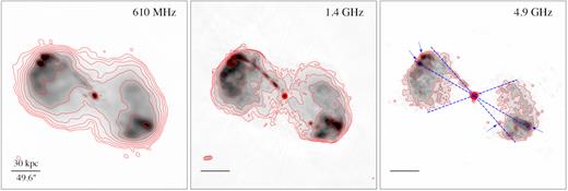
GMRT 610 MHz, VLA 1.4 GHz, and 4.9 GHz images with an rms level of 100, 45, and 112 μJy beam−1 (1σ) and contours of 3C 88 (see Section 2.2 for detail). The GMRT contours start from 5 σ and are spaced by a factor of 2. The 1.4 GHz contours start from 6 σ and are spaced by a factor of 2. The 4.9 GHz contours start from 4.5 σ to 625 σ and the square-root spacing is adopted. The radio images at low and high frequencies show a similar morphology with extended lobes, a narrow jet, and four ‘hotspot'-like features (marked by the blue arrows). The prominent northeastern jet bends near the end, towards the brightest ‘hotspot', while the other ‘hotspot' at the northeast is aligned with the ‘hotspot' at the southwest. The angle between these two blue lines is ∼19°. We also draw a line along the edges of two radio lobes and the angle from it to the radio jet is ∼68°. The radio morphology strongly suggests a jet reorientation projected from roughly east–west to northeast–southwest. The scale-bars in the middle and right panels are the same as the one in the left panel.
This paper is organized as follows. The Chandra and radio observations and data reduction are presented in Section 2. The spatial and spectral analysis are in Section 3. In Section 4, the properties of cavities are discussed. In Section 5, we discussed the warm gas in 3C 88. Sections 6 and 7 contain, respectively, the discussion and the summary of the paper. We assumed the cosmology with H0 = 70 km s−1 Mpc−1, ΩM = 0.3, and ΩΛ = 0.7. At a redshift of z = 0.0302, the angular diameter distance is 124.7 Mpc and 1" corresponds to 0.604 k per cent. All error bars are quoted at 1σ confidence level, unless otherwise specified.
2 Chandra AND RADIO OBSERVATIONS AND DATA ANALYSIS
2.1 Chandra observations
3C 88 was observed by Chandra for ∼105 ks split into three observations (Obs. IDs 11751, 11977, and 12007, PI: Sun) in October 2009 with the Advanced CCD Imaging Spectrometer (ACIS). All three observations (aimpoint on chip S3) were taken in Very Faint (VFAINT) mode and centred on the cool core. The details of the Chandra observations are summarized in Table 1. There was one ACIS-I observation taken in 2008 with a short exposure of ∼11 ks (Sun 2012; Zou et al. 2016). In this study, we focus on the new, deep data with ACIS-S. The data were analysed using the CIAO 4.9 and CALDB version 4.7.4 from Chandra X-ray Center. For each observation, the level 1 event files were reprocessed using CHANDRA_REPRO script to account for afterglows, bad pixels, charge transfer inefficiency, and time-dependent gain correction. The improved background filtering was also applied by setting CHECK_VF_PHA as yes to remove bad events that are likely associated with cosmic rays. The background light curve extracted from a source-free region was filtered with LC_CLEAN script1 to identify any period affected by background flares. There were no strong background flares for all observations and the resulting cleaned exposure time is shown in Table 1.
Summary of Chandra Observations of 3C 88 (PI: Sun).
| ObsID | Date Obs | Total Exp | Cleaned Exp |
|---|---|---|---|
| (kses) | (ks) | ||
| 11977 | 2009 Oct 06 | 49.62 | 49.13 |
| 11751 | 2009 Oct 14 | 19.92 | 19.44 |
| 12007 | 2009 Oct 15 | 34.62 | 33.77 |
| ObsID | Date Obs | Total Exp | Cleaned Exp |
|---|---|---|---|
| (kses) | (ks) | ||
| 11977 | 2009 Oct 06 | 49.62 | 49.13 |
| 11751 | 2009 Oct 14 | 19.92 | 19.44 |
| 12007 | 2009 Oct 15 | 34.62 | 33.77 |
The point sources were detected in the combined 0.5–7.0 keV count image using the CIAO tool WAVDETECT, with the variation of the point spread function across the field considered. The detection threshold was set to 10−6 and the scales are from 1 to 16 pixels, increasing in steps of a factor of |$\sqrt{2}$|. All detected sources were visually inspected and masked in the analysis. The weighted exposure map was generated to account for quantum efficiency, vignetting, and the energy dependence of the effective area assuming an absorbed APEC model with kT = 1.0 keV, NH = 1.12 × 1021 cm−2, and abundance of 0.3 Z⊙ at the redshift z = 0.0302 in the 0.7–2.0 keV. The instrumental background was estimated using the stowed background, which contains only the particle background. The blank sky files contain both the particle background and the cosmic X-ray background. Rescaling blank sky background to remove the particle background may over- or under-estimate the cosmic X-ray background, and would generally require a double-subtraction. While the stowed background includes only the particle background, we can remove it and then model local X-ray background. In our studies, we preferred the stowed background. For each observation, the standard stowed file for each chip was reprojected to match the time-dependent aspect solution, and normalized to match the count rate in the 9.5–12.0 keV band.
Proper background modelling is essential for spectral analysis, especially in low-surface brightness regions. Since the diffuse emission from the galaxy group 3C 88 does not extend over the entire field of view, the region beyond ∼8′ from 3C 88, where the surface brightness is approximately constant as shown in Fig. A1, can be used to model the local X-ray background. For each observation, we extracted the spectrum from the region (>9′) from ACIS-S1, ACIS-S2, and ACIS-I chips separately (I2 and I3 chips are also active for our ACIS-S observations), since the CCD response varies for different chips. All nine spectra were fitted simultaneously with two thermal components at solar abundance and zero redshift plus an absorbed power law with an index of 1.5 to determine the ‘local' X-ray background from this region in our observations. One thermal component is unabsorbed with the temperature fixed at 0.1 keV to account for the emission from the Local Hot Bubble (Snowden et al. 1998; Sun et al. 2009; Liu et al. 2017), the other thermal component is absorbed with the temperature allowed to vary to account for the emission from the Galactic halo. The absorption model is TBABS with a fixed column density of NH = 1.12 × 1021 cm−2. All normalizations are allowed to vary. The best fitting model gives the Galactic halo temperature of |$kT = 0.20^{+0.01}_{-0.02}$| keV. We also compared the derived soft X-ray background flux with the ROSAT All-Sky Survey (RASS) R45 values around the galaxy group (see details in Sun et al. 2009). We found the observed soft X-ray background flux of |$2.94^{+0.37}_{-0.34}\times 10^{-12}$| erg s−1 cm−2 deg−2 in the 0.47–1.21 keV band and R45 value of 113.3 ± 8.0, which is consistent with the relation in fig. 2 of Sun et al. (2009). For spectral fitting, we used XSPEC version 12.9.1 and AtomDB 3.0.8, assuming the solar abundance table by Asplund et al. (2009).
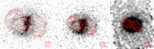
Left: The combined background-subtracted, exposure-corrected Chandra image of 3C 88 in the 0.5–3.0 keV band, smoothed with a 2D Gaussian 9-pixel kernel (0.492″/pixel) and overlaid with the VLA 1.4 GHz radio contours (in red as in Fig. 1). The X-ray point sources have been removed and filled with the local background. The radio contours show a narrow jet, two bright radio lobes, and hotspots on each side of the radio nucleus. The prominent eastern X-ray cavity does not fully overlap with the brightest part of the radio lobe. Middle: The same Chandra image as in the left panel smoothed with a 2D Gaussian 8-pixel kernel (0.984″/pixel). The image shows the prominent cavity to the east of the central AGN, the surrounding bright rims, and the edges associated with the cavity. X-ray decrement to the west is also likely in the position of the radio lobe. Right: The same Chandra image further zoomed out, smoothed with a 2D Gaussian 5-pixel kernel (3.936″/pixel), to show the elliptical edge just outside of the radio lobes. It is identified as a weak shock in this paper.
We also examined the X-ray absorption column density towards 3C 88. The weighted column density of the total Galactic hydrogen is 1.12 × 1021 cm−2 (versus the weighted HI column density of 0.79 × 1021 cm−2), calculated by the ‘NHtot' tool2 including both the atomic hydrogen and the molecular hydrogen column density (Willingale et al. 2013). We fitted the spectra extracted from a circular region of radius 6′ centred on the central AGN for each observation (the central 1.5′ was excluded). The model includes an absorbed thermal component for the diffuse emission from the group plus the diffuse X-ray background component. The background was modelled and re-scaled based on the local X-ray background estimation. The absorption parameter, the temperature, abundance, and the normalization of the source component were allowed to vary. We obtained the best-fitting value of NH = 1.21 ± 0.16 × 1021 cm−2, which is consistent with the weighted total hydrogen column density. We found that our results are not very sensitive to the value of the column density, e.g. the uncertainties of the temperature and the Mach number are generally within 5 per cent, and in some cases ∼10 per cent.
2.2 Radio observations
3C 88 was observed with the GMRT at 610 MHz on 2010 May 7 (project 18_009, PI: Sun). The data were collected using the software correlator and default spectral-line observing mode. The data sets were calibrated and reduced using the NRAO Astronomical Image Processing System package (AIPS) as described in Giacintucci et al. (2011). Self-calibration was applied to reduce residual phase variations and improve the quality of the final images. Due to the large field of view of the GMRT, we used the wide-field imaging technique at each step of the phase self-calibration process to account for the non-planar nature of the sky. The final image was produced using the multi-scale CLEAN implemented in the AIPS task IMAGR, which results in better imaging of extended sources compared to the traditional CLEAN (e.g. Greisen, Spekkens & van Moorsel 2009). The final image at 610 MHz has a resolution of 7.1″ × 5.4″ and an rms noise level (1σ) of 100 μJy beam−1 (Fig. 1). A total flux of 8.8 ± 0.7 Jy is measured for 3C 88 in this image.
NRAO VLA observations of 3C 88 were obtained on 2011 April 15 as part of program SB0517 (PI: Sun). Data presented in this paper were taken in the VLA B configuration with two tunings of bandwidth 128 MHz each centred on frequencies of 1327 and 1455 MHz. The data were observed in spectral-line mode. The observations were calibrated within a modified Common Astronomy Software Applications (CASA) pipeline in version 5.1.2–4 of CASA following standard calibration procedures. Minor modifications to the pipeline were required to enable it to accurately recognize observing intents for calibrators. The flux scale was set using 3C 48. The imaging was undertaken using the multiscale cleaning to accurately recover emission on scales relevant to the source structure. Imaging algorithms also included both multifrequency synthesis with two Taylor terms to more accurately represent the spectral dependence of the emission and w-projection to enable wide-field imaging corrections for non-coplanar effects. The image presented in Fig. 1 has a resolution of 3.9″×3.7″ and an rms level of 45 μJy beam−1 (1σ).
We also show the archival VLA image at 4.9 GHz in Fig. 1. The observation was taken on Apr. 22, 1984 with the C configuration. This image was produced as part of the NRAO VLA Archive Survey, (c) AUI/NRAO.3 The beam size is 4.30″ and the rms level is 112 μJy beam−1 (1σ).
3 SPATIAL AND SPECTRAL ANALYSIS
3.1 Image analysis and radial profiles
We reprojected and summed the count images, background images, and exposure maps, respectively, from three observations using the CIAO tool reproject_image. Fig. 2 (left) shows the combined background-subtracted, exposure-corrected image overlaid with the VLA 4.9 GHz radio contours. Fig. 2 (middle) is the zoomed-out image to show the prominent cavity to the east of the central AGN and the surrounding bright rims. Fig. 2 (right) shows the further zoomed-out image with high contrast to highlight the shock edges.
The images show one prominent cavity at ∼28 k per cent (projected distance) to the east of the nucleus with surrounding bright rims. The cavity does not fully overlap with the brightest part of the radio lobe. The current radio jets and hotspots are not aligned with the cavity and have passed through it to larger radii, at least in projection. Beyond the bright rim of the cavity, there is a sharp surface brightness edge at ∼65 k per cent to the south and north and at ∼80 k per cent to the east and west. As shown in the next section, the gas temperature drops outwards across the edge, which rules out the possibility that the edge is due to a cold front.
To examine if the surface brightness edge surrounding the cavity is consistent with a shock discontinuity, we extracted the surface brightness profiles in the 0.7–2.0 keV band in the same ellipse region from four different wedges to match the shock edge. The centre is chosen to coincide with 3C 88’s radio nucleus. As shown in the top left-hand panel in Fig. 3, the angles (measured counterclockwise from the west) are 145°–240° for the eastern wedge, 240°–305° for the southern wedge, 305°–400° for the western wedge, and 40°–145° for the northern wedge. We also extracted the averaged surface brightness profile within the full ellipse. We used the semimajor axis of the ellipse as the X-axis for all the surface brightness profiles. The particle background was subtracted using the normalized stowed background. We modelled the sky background (see Section 2) and estimated a flux of 1.8 × 10⁻⁷ count s−1 arcsec−2 which is subtracted from the surface brightness. The radial bins were chosen to ensure a minimum of 200 source counts per bin for the averaged surface brightness profile, and a minimum of 100 source counts per bin for those from four wedges. From the surface brightness profile, the X-ray emission from the galaxy group is traced to ∼220 k per cent. We can clearly see the depression of surface brightness in the eastern wedge from ∼5–50 kpc because of the prominent X-ray cavity (Fig. 3 bottom left).
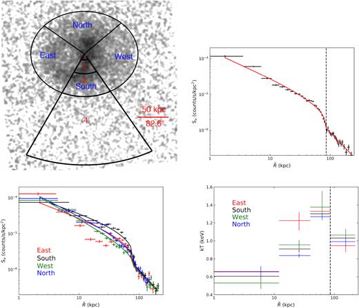
Top left: The combined background-subtracted, exposure-corrected Chandra images of 3C 88 in the 0.7–2.0 keV band, smoothed with a 2D Gaussian 10-pixel kernel (0.984″pixel). The surface brightness profiles are extracted in the same ellipse region from four wedges, with angles (measured counterclockwise from the west) of 145°–240° for the eastern wedge, 240°–305° for the southern wedge, 305°–400° for the western wedge, and 40°–145° for the northern wedge. The ellipse shown in the image has a semimajor axis of 85.7 k per cent and a major to minor axial ratio of 1.26. The regions marked in red are used for spectral analysis (we only show regions in the southern wedge). |$\tilde{R}$| denotes the semimajor axis of the ellipse. Top right: The averaged surface brightness profile across the edge in the 0.7–2.0 keV band. The red solid line shows the best-fit surface brightness model for an ellipsoidal emissivity edge. The vertical dashed line shows the position (semimajor axis of ∼85 k per cent) of the shock edge. Bottom left: The surface brightness profiles in the 0.7–2.0 keV band for the four sectors shown in the top left-hand panel. The solid lines show the best-fit surface brightness model. Bottom right: the deprojected temperatures in region 1, 2, 3 and 4 for four wedges.
Results of shock edge analysis.
| Region | redge | |$p_{\rm i}^{a}$| | |$p_{\rm o}^{b}$| | |$R_{\rm em}^{c}$| | Density Jump | Md | Temperature Jump | Me |
|---|---|---|---|---|---|---|---|---|
| (kpc) | ||||||||
| East | 81.26 | 0.79 ± 0.32 | 1.37 ± 0.22 | 3.72 ± 1.38 | 1.48 ± 0.51 | 1.33 ± 0.36 | 1.40 ± 0.10 | 1.41 ± 0.10 |
| West | 80.37 | 0.95 ± 0.03 | 1.42 ± 0.13 | 1.98 ± 0.42 | 1.79 ± 0.19 | 1.56 ± 0.15 | 1.29 ± 0.14 | 1.30 ± 0.14 |
| South | 82.45 | 0.75 ± 0.06 | 1.42 ± 0.09 | 4.80 ± 0.85 | 1.89 ± 0.24 | 1.64 ± 0.20 | 1.26 ± 0.06 | 1.27 ± 0.06 |
| North | 86.32 | 0.90 ± 0.04 | 1.52 ± 0.25 | 4.80 ± 0.85 | 1.87 ± 0.47 | 1.62 ± 0.38 | 1.28 ± 0.08 | 1.30 ± 0.09 |
| Full | 85.73 | 0.87 ± 0.02 | 1.37 ± 0.06 | 3.11 ± 0.30 | 1.57 ± 0.31 | 1.39 ± 0.23 |
Note: a: the inner slope of emissivity power law; b: the outer slope of emissivity power law; c: the emissivity jump at the edge; d: Mach number from density jump; e: Mach number from temperature jump; see Section 3.1 for detail.
3.2 Spectral analysis
3.2.1 Radial spectral analysis
Spectra were extracted from the same circular annuli for the three observations separately using the CIAO tool specextract. For each spectrum, the weighted response files and matrices were made, and a corresponding background spectrum was extracted from the same region from the normalized stowed background data. The sky background model obtained from the local background estimation (Section 2) was scaled by the area of each region and subtracted. The spectra were fitted in the energy range 0.5–5.0 keV with XSPEC 12.9 using the C-statistic. The spectra from the same region from three observations were fitted simultaneously to an absorbed thermal APEC model, i.e. TBABS*APEC. The temperature, metallicity, and the normalization were allowed to vary freely. For regions where the abundances cannot be well constrained due to the fewer counts, we fixed it at the best-fitting value or at the value obtained in nearby regions.
We focused our analysis on the ACIS-S3 chip and extracted a set of 11 circular annuli from the centre to a radius of ∼220 kpc. The deprojected temperature profiles are shown in Fig. 4 (top left). For temperature deprojection, we adopted a model-independent approach (e.g. Dasadia et al. 2016) assuming spherical symmetry and the cluster temperature is uniform in each spherical shell. The approach is very similar to the ‘onion-peeling” method, but with a different way to estimate the emission contribution to each annulus from the outer spherical shells. We used Monte Carlo simulations to populate the 3D shells and create the projected images where each pixel represents the number of events that fell within each shell. By applying the respective masks (e.g. the included and excluded regions) to the simulated images, we can calculate the emission contribution factor from the outer spherical shell based on the sum of the pixel values. Using this method, we can account for point sources and chip gaps. We noted that our results are consistent with the results obtained by using the PROJCT model in XSPEC.
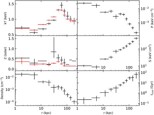
The azimuthally averaged radial profiles of the deprojected temperature, abundance Z, electron density, pressure, entropy, and cooling time. For comparison, we also show the projected temperature and abundance profiles in red.
The deprojected temperature profile increases from ∼0.6 keV in the centre (within 10 k per cent) up to 1.45 keV at ∼62 k per cent (∼0.1r180, r180 is the virial radius and rΔ is defined as the radius where the mean mass density equals to Δ times of the critical density.), then declines towards large radii. This behaviour is very similar to the temperature profiles observed in other galaxy groups (e.g. Gastaldello et al. 2007; Sun et al. 2009). We noticed that the temperature peak is located just inside the shock region, which may complicate the detection of the actual temperature jump due to the shock itself, as found in other systems, e.g. in Hydra A (Gitti et al. 2011). The abundances (Fig. 4 middle left) are not well constrained in a few annuli and therefore are fixed. The abundance within ∼20 k per cent is relatively flat at a low value of ∼0.3. The low abundance at the centre of cooling flow clusters is mainly due to fitting multiple temperature spectra with a single thermal model (the so-called ‘Fe bias' effect, Buote 2000). The abundance in the fifth data bin where the cavity is located shows a jump, but with a large uncertainty.
We also present various quantities in Fig. 4. The electron density was obtained directly from the deprojected normalization of the APEC component assuming ne = 1.22nH, where ne and nH are the electron and proton densities. A dip is shown in the density profile at ∼28 k per cent corresponding to the location of the cavity (Fig. 4 bottom left). Based on the deprojected gas temperature and density, we calculated the pressure in each annulus as P = nkT (where n = 1.92ne) and the entropy as |$S=kT/n_{\rm e}^{-2/3}$|. As shown in Fig. 4 middle right, the entropy profile declines all the way to the centre. The entropy profile can be well represented by a constant plus a power law as S = S0 + S1(r/100 kpc)p, with the best-fitting slope of 1.19 ± 0.09 and the central entropy floor S0 = 7.31 ± 1.68 keV cm2. We found the best-fitting entropy slope of 0.79 ± 0.07 between 30 k per cent and 0.15r500, which is consistent with the values found in galaxy groups and clusters (e.g. Sun et al. 2009), and the slope of 1.19 ± 0.05 between 0.15r500 and r2500 (e.g. 65–206 k per cent).
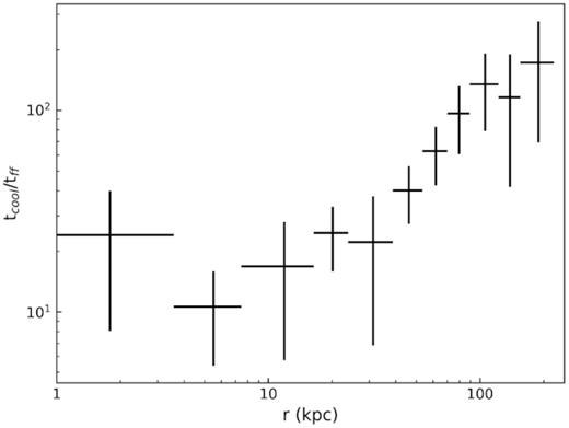
Radial profile of tcool/tff.
3.2.2 Temperature and abundance map
To study the thermal structure of the group, we performed a 2D spectroscopic analysis using contour binning (Sanders 2006). We generated 32 regions with a signal-to-noise ratio of 50 for 3C 88 using counts image in 0.7–2.0 keV band. We used the model TBABS*APEC to model the gas emission in each region in 0.5–5.0 keV band. The resulting projected temperature and abundance maps are shown in Fig. 6. The temperature map shows the high-temperature region surrounding the eastern cavity, at the location of the shock edges. The abundance map shows low-abundance regions close to the central AGN, which again is possibly due to the ‘Fe bias', and the high-abundance regions surrounding the cavity, which we will discuss later in Section 6.6.

3.2.3 Shock spectral analysis
4 THE X-RAY CAVITY
In Fig. 2 (left) the smoothed Chandra X-ray image of 3C 88 shows a pronounced cavity to the east of the core, which is also evident from the surface brightness profile extracted from the eastern wedge as in Fig. 3. The corresponding cavity to the west is not significant.
We estimated the lower limit of the total jet power based on the enthalpy and buoyant rise time of the cavities (Churazov et al. 2001), to ensure the direct comparison with previous studies. We assume the cavity has a spherical geometry centred at 3:27:57.327, + 2:33:33.623 with a radius of 0.633′. The projected distance of the centre of the eastern cavity to the nucleus is ∼28 k per cent, with a radius of 23 k per cent. The buoyant rise time of the bubble is calculated at its terminal velocity ∼(2gV/SC)1/2, where V is the volume of the bubble, S is the cross-section of the bubble, and C = 0.75 is the drag coefficient (Churazov et al. 2001). The gravitational acceleration is calculated as g ≈ 2σ2/R, with the central stellar velocity dispersion of 189 km s−1 (Smith, Heckman & Illingworth 1990). Thus, the age of the bubble to its present position is 6.0 × 10⁷ yr. The total cavity enthalpy (H = 4PV, where P is the azimuthally averaged pressure at the radius of the centre of the cavity) is calculated from the deprojected temperature and the electron density profile. The total enthalpy and the cavity power for the eastern are 3.8 × 1058 erg and 2.0 × 1043 erg s−1. We noted that the cavity power to the cooling luminosity ratio is ∼61, showing that the mechanical power is sufficient to offset the cooling. If we instead use g at the centre of the cavity derived from Section 3.2, the age of the bubble is ∼40 per cent lower and the resulting cavity power is ∼60 per cent higher.
The spectra in Fig. 7 were extracted from each observation of the eastern cavity region (see Fig. 2), together with response files and background spectra. We fitted the spectra with a one temperature model as TBABS*APEC and obtained the best fitting projected temperature of |$1.22^{+0.06}_{-0.07}$| keV and the abundance of |$0.22^{+0.09}_{-0.06}$| solar. Although the one temperature model provides a good fit to the spectra, it is lower than the data above ∼3 keV as shown in Fig. 7. Thus, we added another thermal component to place constraints on any hot gas in the cavity. We fixed the temperature of the first thermal component to 1.05 keV at the radius of the cavity obtained from the projected fitting to account for the projected emission. The second component accounts for any thermal emission inside the cavity. The temperature is constrained between 1.5 and 10 keV. The metallicities of the two components are tied together.
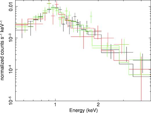
Spectra at the position of the eastern cavity from three observations, with the best-fit single temperature model (see more detail in Section 4).
We found that adding a hotter component improves the fit with a significance of 99 per cent using F-test, implying the existence of hot gas in the cavity. Assuming the hot gas in the cavity is in pressure balance with the cooler gas, we can place constraints on the volume-filling factor based on the temperature and normalizations of the cool and hot gas. We found that, as the temperature of the second component increases, the metallicity increases and reaches above ∼1.0, which is a typical value for group centres. This may be the result of ‘Fe bias', which typically occurs when fitting a single-temperature model to the spectrum of the multiphase gas. The volume-filling factor increases rapidly from 0.72 for 1.5 keV to 0.99 for temperatures greater than ∼5.5 keV.
5 WARM GAS IN 3C 88
Narrow-band imaging data on 3C 88 were taken on December 16, 2009, with the Seaver Prototype Imaging camera (SPIcam) on the Astrophysical Research Consortium 3.5-m telescope at the Apache Point Observatory. SPIcam is a general purpose, optical imaging CCD camera with a field of view 4.78′ square. Two 900 s Hα + [N ii] observations were taken with the NMSU-677.6 filter (central λ: 6776 Å, width: 75Å). Two 540 s observations with the NMSU-665 filter (central λ: 6650 Å, width: 80Å) were taken for the continuum (or Hα off). Both filters are 2 inch square, so only the central ∼3′ square is unvignetted. The seeing was ∼1.1″ and the sky was photometric during our observations.
We follow the standard CCD analysis for the SPIcam data. Dome flats were used and the spectrophotometric standard was Feige34. The Galactic extinction was 0.259 mag for the NMSU-665 filter and 0.252 mag for the NMSU-677.6 filter, with the extinction law from Fitzpatrick (1999) and assuming RV = 3.1. A software issue with the SPIcam shutter in 2007 – 2010 adds 0.7505 s to the requested exposure. This was identified at the end of 2010 and was corrected for our analysis.
For continuum subtraction, we generally follow the isophote fitting method described in Goudfrooij et al. (1994), by studying the Hα / off ratio profile. The net Hα + [N ii] emission of the galaxy is shown in Fig. 8. 3C 88 hosts a nuclear source with Hα + [N ii]. A diffuse extension, beyond the nuclear source, is detected to at least 5 k per cent from the nucleus. The presence of multiphase gas with ∼5 k per cent extent (and fairly low tcool compared with the free-fall/eddy time-scales; Sec. 3.2.1) can be understood in the CCA scenario (cf. Gaspari et al. 2018), in which cold/warm gas originates from the in situ condensation cascade and recurrently triggers the AGN jets. Further away from the nucleus, a compact knot is detected 16 k per cent NE of the nucleus, with potentially a faint filament to its north. Within the central 6 k per cent radius, where most of the central diffuse emission lies, we measure a total Hα luminosity of 6.6 × 1039 erg s−1, assuming no intrinsic extinction. The small blob, 16 k per cent NE of the nucleus, has a total Hα luminosity of 5.3 × 1039 erg s−1, if it is associated with 3C 88. The following line ratios are assumed, [N ii]6583/Hα = 1.5 and [N ii]6548/[N ii]6583 = 1/3, which are consistent with the typical values in Goudfrooij et al. (1994). Deeper narrow-band imaging data with good seeing and spectroscopic data are required to better understand the state of warm gas in this system. Nevertheless, 3C 88 does host some warm gas near the nucleus and the radio jet.
![Optical continuum (H α off) and net H α + [N ii] images of the centre with the 3.5m APO telescope. The VLA 4.9 GHz contours (red, same as the ones shown in Fig. 2) and optical contours (green) of the bright part are also shown. There is an H α + [N ii] extension beyond the central nucleus. Blue arrows in the right panel mark a compact emission-line feature (solid blue line) and a potential emission-line diffuse feature (dashed blue line) close to the NE jet, more than 16 k per cent away from the nucleus.](https://oup.silverchair-cdn.com/oup/backfile/Content_public/Journal/mnras/484/3/10.1093_mnras_stz229/2/m_stz229fig8.jpeg?Expires=1750247514&Signature=UK0idjixSqmPG0hPTF3KG3nwOk8oKimNZWGCp4p85wlfQm6QIzdRNCFWFTSOpoylK9KVKLaU-tu-hpdyG~woDA39PKIxNTVjNsbCGr6-VMuR5UqmkZdfs~06~ufgg1JM5rgtoxFweZDuEoZGKknGLFEElr00vDEP0Qho2rDt51o3lrtvKgPt3PZlCvet66YnceXwZHOFEOVxtdggTy8ZxMssxXZrZ6Kguq9XBdkU0Owj-5eI0t56QX5lVXEmA5DUgMwLxGCC8wBEZRZ-AWRCw1KJNYLJYORwIrfQ2VxOpcj5EHnYJ5gmrW2-I0E4XoEoY6xPIIJphpV66J0ujS92oQ__&Key-Pair-Id=APKAIE5G5CRDK6RD3PGA)
Optical continuum (H α off) and net H α + [N ii] images of the centre with the 3.5m APO telescope. The VLA 4.9 GHz contours (red, same as the ones shown in Fig. 2) and optical contours (green) of the bright part are also shown. There is an H α + [N ii] extension beyond the central nucleus. Blue arrows in the right panel mark a compact emission-line feature (solid blue line) and a potential emission-line diffuse feature (dashed blue line) close to the NE jet, more than 16 k per cent away from the nucleus.
Since 3C 88 was not observed by Herschel or Spitzer/MIPS and it was not detected in Galex FUV AIS data, we estimate its SFR solely from the Wise 22μm data. Based on the SFR calibration by Lee, Hwang & Ko (2013), the SFR for 3C 88 is 0.96 M⊙ yr−1 for the Kroupa IMF. However, one can only view this estimate as an upper limit, as the nuclear emission may dominate the 22 μm emission. Star formation in 3C 88 is at most weak.
6 DISCUSSION
6.1 The central AGN
Fig. 9 shows the subpixel (0.0984″/pixel) Chandra X-ray image of the central region. We extracted spectra of the central X-ray source from each observation in a circular region with a radius of 2″, and the background spectra from an annulus from 2″ to 4″. The spectra from the three observations were fitted simultaneously between 0.4 and 8.5 keV. The nuclear spectrum is flat and the power-law photon index is ∼0.6 from a simple power-law model (Table 3). We confirmed that pileup is negligible even for the brightest ACIS pixel. As the local background is simply scaled by the solid angle, the residual thermal emission is expected in the nuclear spectrum. As the spectrum is flat, simply adding a thermal component results in a negligible contribution. We attempted models with an obscured AGN plus a soft component, which indeed improves the fits (Table 3). If the canonical value of 1.7 for the power-law index of the AGN is preferred, 3C 88’s AGN is obscured with a moderate intrinsic absorption column density of ∼2 × 1022 cm−2. The rest-frame 2–10 keV luminosity of the AGN is ∼4 × 1041 erg s−1.

The 0.7–7.0 keV subpixel (0.0984″/pixel) image of the central region, smoothed with a 2D Gaussian 4-pixel kernel. The spectrum of the central AGN is extracted from a circle with a radius of 2″ that is shown in red. Despite the limited statistics of the data, some features are revealed around the centre, including a linear feature to the northeast on the same direction of the radio jet (inner X-ray jet?) and extension to the east and west.
Spectral fits of the central AGN.
| Model | |$\Gamma _{1}\, ^a$| | |$kT/\Gamma _{2}\, ^b$| | |$N_{\rm H, intr}\, ^c$| | |$L_{0.5-2.0}\, ^d$| | |$L_{2-10}\, ^e$| | |${}[C, C_{e}, C_{\sigma }]\, ^f$| |
|---|---|---|---|---|---|---|
| (keV) | (1022 cm−2) | (1040 erg s−1) | (1041 erg s−1) | |||
| tbabs*POW | |$0.60^{+0.04}_{-0.04}$| | |$5.71^{+0.21}_{-0.21}$| | [157.8, 131.0, 16.3] | |||
| tbabs*(ztbabs*POW + APEC) | |$1.40^{+0.14}_{-0.14}$| | |$0.73^{+0.07}_{-0.14}$| | |$1.6^{+0.3}_{-0.3}$| | |$1.78^{+0.23}_{-0.22}$| | |$4.57^{+0.20}_{-0.19}$| | [115.9, 131.1, 16.0] |
| tbabs*(ztbabs*POW + APEC) | 1.70 | |$0.77^{+0.06}_{-0.07}$| | |$2.1^{+0.2}_{-0.2}$| | |$1.97^{+0.23}_{-0.21}$| | |$4.19^{+0.15}_{-0.14}$| | [120.3, 131.4, 15.9] |
| tbabs*(ztbabs*POW + POW) | 1.70 | |$1.13^{+0.22}_{-0.19}$| | |$3.1^{+0.4}_{-0.4}$| | |$2.79^{+0.32}_{-0.36}$| | [118.3, 131.6, 16.4] |
Note: a: the photon index for the first power-law component; b: the temperature for the thermal component (we assumed an abundance of 0.3 Z⊙. The fits are not sensitive to the assumed abundance value.) or the photon index for the second power-law component; c: the column density for the intrinsic absorption; d: the rest-frame 0.5–2.0 keV luminosity for the thermal component; e: the rest-frame 2–10 keV luminosity for the power-law component; f: C, Ce, Cσ are the fitted C-statistic, its expected value, and its standard deviation computed based on Kaastra (2017). 68% of the time the acceptable spectral models should have |$-1\lt \frac{C-C_{e}}{C_{\sigma }} \lt 1$|.
We examined the variability of the central point source based on the flux from the 0.5–10 keV band. As shown in Table 1 the time separations for three observations are ∼7 and ∼1 day. Since the AGN variabilities have different time-scales, we also include the old, short ACIS-I observation (Obs. ID 9391) taken more than 1-year earlier. We found that there are small variations between the four observations and the 0.5–10 keV flux changes by ∼20 per cent. We also checked the possible X-ray emission associated with the radio features, e.g. radio jet and the hot spots. Like Massaro et al. (2015), we chose a circular region for the hot spots and a box region for the radio jet to measure the observed X-ray emission. Background regions of the same shape and size were chosen to avoid emission from other sources, with one box for the radio jet, and two circles for the hot spots. X-ray emission from the radio jet (∼25″ northeast to the nucleus) is detected with a significance of ∼4.0σ, and with a significance level of ∼4.7σ from the eastern hotspot (∼109″ to the nucleus; note that this feature is marked as ‘jet knot” in Massaro et al. 2015). There is no detection of X-ray emission associated with the western hotspot. The hardness ratio (2.0–7.0 keV flux divided by 0.5–2.0 keV flux) of the eastern hotspot is ∼0.17, which corresponds to a power-law index of ∼2.5 assuming an absorbed power-law model. We estimated a 0.5–10 keV X-ray luminosity of 6.0 ± 1.3 × 1039 erg s−1 for the eastern hotspot. Assuming the same spectral shape, we obtained an upper limit luminosity of ∼1039 erg s−1 for the western hotspot.
Based on the core flux density measured by the VLA (Morganti, Killeen & Tadhunter 1993) at 5 GHz, we calculated a radio luminosity at 5 GHz of LR = 1.68 × 1040 erg s−1. Using the black hole Fundamental Plane (Gültekin et al. 2009), or the relation between the radio luminosity at 5 GHz, the X-ray 2–10 keV luminosity, and the black hole mass, we estimated a black hole mass of ∼7.4 × 10⁸ M⊙, which is comparable to the black hole mass of ∼5.0 × 10⁸ M⊙ estimated from the Mbulge − MBH relation (Bettoni et al. 2003).
6.2 Jet/cavity geometry
Fig. 10 is a schematic diagram showing the geometry of the jets and cavities, viewed from the positive z-axis. The jets propagate out from the origin of the 3D axes into cones with half-angle ψ. The angle between the jet and the line-of-sight (LOS) is θ1. Two symmetric cavities lie on each side with an angle of θ2 to the LOS. The jet axis is assumed to be aligned with cavity previously (axis marked as P) and realigned to the current axis (marked as P′).
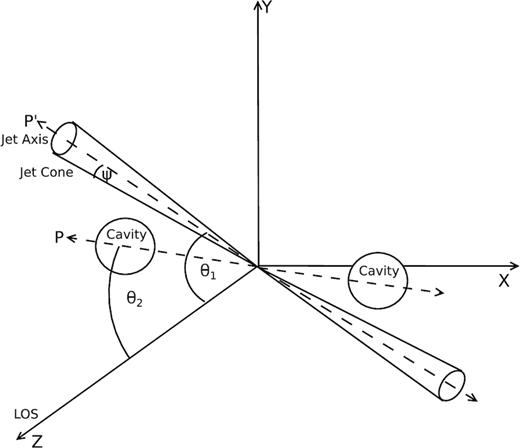
The schematic plot of the jet/counterjet geometry. ψ is the half-jet cone angle, θ1 is the angle between the jet axis and the line-of-sight, and θ2 is the angle between the cavity and the line-of-sight. P is the previous jet axis, and P′ is the current jet axis.
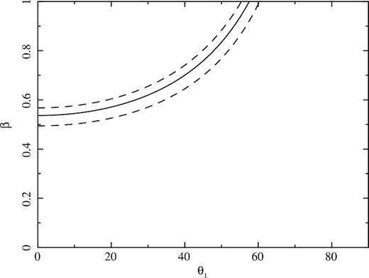
The constraints on the jet speed and the angle to the line-of-sight for the jet to counterjet brightness ratio Rjet of 20 (the solid line). Two dashed lines show the constraints for Rjet of 15 and 25. Only the parameter space above the lines is allowed.
Can the narrow jet produce such a wide cavity as shown in Fig. 2? Here, we list some possibilities. First, the light jets with relativistic cosmic rays (CRs) can create fat cavities. The CR-dominated jets are so light that they are quickly decelerated in the ICM due to their low inertia and momentum, then the CR pressure drives the lateral jet expansion to form fat lobes, which are mainly formed by jet backflows and supported by the CR pressure (Guo & Mathews 2011). Second, the jet intermittency can also help. The recent study shows that multiple jets produce a single, large cavity system if the reorientation angle between two successive jets is small and the time interval is sufficiently short so that they can keep inflating the same cavity (Cielo et al. 2018). This is consistent with the fact that the current radio jet is misaligned with the X-ray cavity in 3C 88. Another possibility to create fat bubbles is through ultrafast outflows (UFOs, v > a few 104 km s−1) (e.g. Sternberg, Pizzolato & Soker 2007; Soker 2016, and references therein). In general-relativistic, radiative magneto-hydrodynamic simulations (GR-RMHD, e.g. Gaspari & Sa̧dowski 2017), the accretion energy is transformed within 100s of gravitational radii into the UFOs, which become more massive at the k per cent scale and decelerate, inflating the bubble and thermalizing the kinetic energy mainly through turbulent mixing.
Previous studies (e.g. Rafferty et al. 2006; Hlavacek-Larrondo et al. 2012) found that the shapes of cavities vary from almost perfectly circular to elongated. Shin, Woo & Mulchaey (2016) found that the shapes of non-circular cavities follow a bimodal distribution, in that cavities are elongated either along the jet direction or perpendicular to the jet direction. In a recent study, Guo (2015) showed that the shapes of young cavities are closely related to various jet properties, e.g. jet density, velocity, energy density, and duration. In general, very light internally subsonic jets produce bottom-wide cavities elongated along the perpendicular direction to the jet, while the heavier internally supersonic jets produce top-wide cavities elongated along the jet direction. The long-term evolution of cavity depends significantly on the viscosity of the hot ICM, and on the amount of entrainment along the jet/outflow path from the per cent to 10 k per cent scale. From Fig. 2, the eastern cavity in 3C 88 appears more elongated in the direction perpendicular to the jet (although projection effects may make the cavities appear more circular). However, the cavity is located away from the jet axis and the angle between the jet axis and the radial direction from the AGN centre to the cavity centre is ∼50°. This is suggested to be due to jet reorientation (see Section 6.3), which makes it hard to infer the jet properties directly from the cavity shape.
The region of the eastern cavity seen in Fig. 2 can be approximated as a circle with a radius of 23 k per cent, projected at a distance of 28 k per cent from the AGN. Assuming that the cavity is a sphere in 3D space, we can make a rough estimate of the angle between the LOS and the cavity. For an angle θ2 between the LOS and cavity, the real distance of the cavity to the centre is therefore 28 k per cent/sin(θ2). We first simulated the 3D gas distribution with its temperature and density following the deprojected profiles. The cavities are assumed to be spheres devoid of the gas. Then, we projected the simulated data on the sky plane with a different angle θ2. We used two circular regions with the same size, with one free of the cavity and the other overlaid with the projected cavity, and calculated their surface brightness ratio. As expected, we found that the surface brightness ratio increases with the angle θ2, e.g. the surface brightness ratio increases by about ∼50 per cent as θ2 ranges from 30° to 90°. We can place constraints on the angle θ2 based on the surface brightness ratio, e.g. a threshold of 1.1 giving a lower limit on θ2 = 32°. Notice that in real observations, the surface brightness contrast between the ambient region and the cavity region is more striking due to the bright surrounding rims or enhancements, with a much larger surface brightness ratio than in our simulations.
6.3 Jet reorientation
With deep X-ray observations, systems with multiple pairs of X-ray bubbles (or cavities) at different positional angles have been observed (e.g. Bogdán et al. 2014; Randall et al. 2015). One scenario for the formation of multiple pairs of X-ray bubbles is jet reorientation model, in which the jet axis was initially along the direction of one pair of bubbles, and along a different direction later (the jet activity may switch off before changing directions). The jet reorientation models include the conical precession, which reproduces well the observed radio structures in some radio sources (e.g. Gower et al. 1982; Cox, Gull & Scheuer 1991; Dunn, Fabian & Sanders 2006), and other realigning mechanisms, e.g. due to the binary black hole merger or the instabilities of accretion disc (e.g. Dennett-Thorpe et al. 2002; Gopal-Krishna et al. 2012). 3C 88 provides a great case to study jet reorientation and two methods are discussed in this section.
6.3.1 Method I: X-ray cavity + radio jet
6.3.2 Method II: radio jet curvature
In Fig. 1 the northeastern radio jet starts to bend at a projected distance of ∼55 k per cent with a deflection angle of ∼15°. Two hotspots at the northeast and at least one hotspot at the southwest are detected. This type of radio morphology, also observed in other systems, (e.g. 3C 123, Cygnus A) can be explained by jet reorientation (e.g. Cox et al. 1991; Steenbrugge & Blundell 2008; Pyrzas, Steenbrugge & Blundell 2015). In this scenario, the jet initially strikes the wall of the cocoon producing the jet curvature as it feeds the primary hotspot. The jet then interacts with the cocoon at a very sharp angle and generates a new primary. The old primary is then observed as a secondary hotspot. In this picture, the radio jet of 3C 88 was previously lying in the direction from the nucleus to the secondary hotspot, and it is currently aligned with the observed radio jet.
Based on the eastern bent jet we can make a rough estimation of the time-scale. As seen in the radio image, the narrow radio jet maintains its width and does not widen even at a large radius (∼55 kpc). We do not expect a significant jet deceleration due to the low ICM density and expected low stellar mass loss rates. Therefore, the jet remains relativistic until it is close to the hotspot. Assuming a constant speed of ∼0.5c (see Fig. 11) for jet travelling from the centre to 55 k per cent, and a lower speed from the bent point to the hotspots, we can estimate the traveltime, which depends mostly on the latter speed. Assuming a jet speed of 0.01c or 0.05c (e.g. Scheuer 1995; Carilli & Barthel 1996), we obtained a traveltime of 4.3 Myr or 1.2 Myr, corresponding to a jet reorientation rate of 4° or 15° per Myr.
We notice that the estimated jet reorientation rates from two methods differ a lot, since they are probing different epochs, e.g. method I probes the average rate whereas method II probes the instantaneous one. The origin of jet reorientation is likely tied to the accretion history of the central SMBH. An intriguing scenario is related to the transition between FR I and FR II radio sources (e.g. Garofalo, Evans & Sambruna 2010). On the other hand, in the framework of the CCA, warm/cold clouds and filaments collide inelastically, which can boost the accretion rate and suddenly alter the SMBH spin and thus the jet orientation (e.g. Gaspari et al. 2012). In fact, only CCA can likely drive such a large variability able to alter rapidly the BH spin: this is because of the random orientation of the raining clouds (see also King & Pringle 2006; King, Pringle & Hofmann 2008). Hot accretion is too smooth to rapidly change the spin (and is also spherically symmetric); disc-driven jets have quite fixed orientation perpendicular to the disc and it takes very long time to alter the disc morphology and fully change its direction as in a merger (rather than accreting different already inclined clouds as in CCA).
6.4 Cavity power in radio loud groups
X-ray cavities provide a direct estimate of the power output of the central AGN, from the cavity enthalpy (the minimum energy required to form a cavity) and the time-scale over which the cavity has formed. The mechanical power of the cavities is found to be correlated with the AGN radio luminosity, e.g. Pradio − Pcav relation (Bîrzan et al. 2008; Cavagnolo et al. 2010; O’Sullivan et al. 2011). In general, a large cavity power is expected for luminous radio galaxies. However, as shown in Fig. 12, the cavity power found in radio-loud galaxy groups (e.g. P1.4GHz ∼ 1–10 × 1024 W Hz−1, and kT < 1.3 keV) in the previously studied samples (e.g. Bîrzan et al. 2008; Cavagnolo et al. 2010; O’Sullivan et al. 2011) is less than 1043 erg s−1. For 3C 88 with L1.4GHz ∼ 1025 W Hz−1, we measured the total mechanical power of cavities of ∼2 × 1043 erg s−1, which is at least two or three times higher than what is found in other radio luminous groups, except for PKS B2152-699 (Worrall et al. 2012). The cavity power of PKS B2152-699 is ∼3 × 1043 erg s−1 using the dynamical time, or ∼1 × 1043 erg s−1 using the buoyant rise time as for 3C 88. In either case, the cavity power of the two radio luminous galaxy groups, 3C 88 and PKS B2152-699, are comparable. X-ray cavities in PKS B2152-699 are over two times smaller than 3C 88’s in radius as 3C 88’s X-ray cavity is the largest known in galaxy groups.
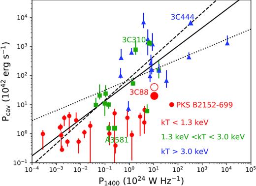
Cavity power versus radio power at 1.4 GHz for galaxy groups and clusters (red: kT < 1.3 keV, green: 1.3 < kT < 3.0 keV, blue: kT > 3.0 keV) from Bîrzan et al. (2008), Cavagnolo et al. (2010), and O’Sullivan et al. (2011). The dotted, dashed, and solid lines are the best-fitting relations from their work, respectively. For some repetitive systems, we used the values from O’Sullivan et al. (2011). The differences in cavity power are generally within a factor of 2 for all repetitive systems, except for NGC 6269, whose cavity power is about seven times smaller in Cavagnolo et al. (2010). New studies on NGC 5813 found three pairs of X-ray cavities (Randall et al. 2011, 2015). However, the total cavity power is consistent with the value used in the plot. We included four additional systems, PKS B2152-699 (Worrall et al. 2012, the cavity power is estimated using the buoyant rise time as for other systems in the plot), 3C 310 (Kraft et al. 2012), 3C 444 (Croston et al. 2011) and Abell 3581 (Canning et al. 2013) in the plot. The large solid red circle denotes the location of 3C 88, whose cavity power is among the largest in galaxy groups (please see Section 6.4 for discussion). The empty red circle represents 3C 88 assuming there are a pair of cavities with the same power.
If the cavity centre does not lie in the plane of sky, we need to estimate the projection effect on the estimated cavity power. Since the actual distance from the AGN to the centre of cavity and the size of cavity would increase, the pressure at the centre of cavity would be lower, while the volume of cavity would increase, hence affecting the estimation of total enthalpy. In addition, the estimated age of the cavity will increase. Assuming a low limit of ∼30° for inclination angle θ2, we obtained a new cavity power of 5 × 1043 erg s−1.
Despite the uncertainties in estimating the cavity powers, e.g. the estimation of the cavity volume, a natural question is why the measured cavity powers in groups are generally low, even for those radio luminous systems. Sun et al. (2009) showed that groups with a luminous cool core (L0.5 − 2keV ≥ 1041.7 erg s−1) do not host luminous radio AGN (L1.4GHz > 1024 W Hz−1). The groups with luminous radio AGN only have small coronae or small cool cores, so the extended X-ray atmosphere that encloses the radio lobes is faint. As both cavities and shocks are easier to detect in high-density regions, these features become subtle in groups, especially for groups hosting strong radio AGN. The Chandra constraints on the cavity power may only include the power deposited in cool cores and the estimated power should be taken, generally, as a lower limit.
6.5 Shock energy
Using an ellipsoidal geometry for the volume contained within the shock front with semi-major and semi-minor axes of 85.7 kpc and 68.0 kpc (as shown in Fig. 3) and the azimuthally averaged pressure profile from Fig. 4, we estimated a shock energy of 1.9 × 1059 erg. To make a comparison, we checked through the literature for the systems with available Mach numbers, shock energies, and cavity enthalpies, e.g. Hydra A (Nulsen et al. 2005b; Wise et al. 2007), MS 0735 + 7421 (McNamara et al. 2005; Vantyghem et al. 2014), Centaurus A (Croston et al. 2009), Cygnus A (Bîrzan et al. 2004; Snios et al. 2018), 3C 444 (Croston et al. 2011), M87 (Churazov et al. 2001; Forman et al. 2005, 2007, 2017), Abell 2052 (Blanton et al. 2009), 3C 310 (Kraft et al. 2012), NGC 4552 (Machacek et al. 2006), NGC 4636 (Baldi et al. 2009), HCG 62 (Gitti et al. 2010), NGC 5813 (Randall et al. 2011, 2015, notice NGC 5813 shows three distinct AGN outbursts.). In Fig. 13 (left), we show the Mach number versus shock energy. The shock energies span almost 7 orders of magnitude, with a shock energy of 4 × 1061 erg for MS 0735 + 7421 and ∼1055 erg for NGC 4552, while the Mach numbers range from 1–2, except for Centaurus A. The shock energy in 3C 88 is the largest among the low temperature groups. Although it has a similar Mach number and shock radius to 3C 88, Cygnus A, by far the nearest powerful radio galaxy, has a shock energy about 20 times larger than that of 3C 88. In Fig. 13 (right), we show the cavity enthalpy versus the shock energy. Either shock energy or cavity enthalpy can be the most significant form of mechanical energy produced by AGN outbursts, with their ratio generally varying within 0.1–10.0. In 3C 88, the ratio of the shock energy to the total cavity enthalpy is about 5.0.
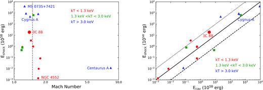
Shock energy versus Mach number (left) and shock energy versus cavity enthalpy (right) for galaxy groups and clusters (red circle: kT < 1.3 keV, green square: 1.3 < kT < 3.0 keV, and blue triangle: kT > 3.0 keV) from the literature (see details in Section 6.5). The dashed line on the left panel represents Mach number = 1.5. The dotted, solid, and dashed lines on the right panel represent Eshock/Ecav = 10, 1, and 0.1, respectively. The large red circle denotes 3C 88.
6.6 Bright rims and arms
The abundance map shown in Fig. 6 suggests enhanced abundance along the eastern bright rim and arm. Several interesting regions with enhanced X-ray surface brightness are defined in Fig. 14. There are two possible explanations for the presence of the enhanced X-ray features. One explanation is the rims could be shells of gas shocked during the supersonic expansion of the bubbles (e.g. Fabian et al. 2003; Forman et al. 2007). Alternatively, if the bubbles are rising in a subsonic phase of expansion, the dense and cool gas from the cluster centre could be lifted by the rising bubbles (as in, e.g. M87: Churazov et al. 2001, Simionescu et al. 2008, Hydra A: Kirkpatrick et al. 2009, Gitti et al. 2011; Werner et al. 2010; NGC 4472: Gendron-Marsolais et al. 2017; NGC 1399: Su et al. 2017).
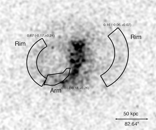
0.7–2.0 keV Chandra image of 3C 88 to show the regions and the measured abundances that are discussed in Section 6.6.
The spectra for each region, from all three observations, were then fitted simultaneously with the model TBABS*APEC with fixed absorbing column density. We found temperatures of |$1.36^{+0.10}_{-0.03}$| and |$1.33^{+0.21}_{-0.07}$| keV for the eastern and western rims, respectively, which are higher than those from adjacent regions. The metallicity in the western rim is |$0.16^{+0.07}_{-0.06}$| solar, while it is |$0.67^{+0.24}_{-0.17}$| in the eastern rim. The metallicity enhancement surrounding the eastern cavity implies that the hot, metal rich gas was lifted by the rising X-ray bubble from the group centre (e.g. Kirkpatrick & McNamara 2015). The relation between the radius of the eastern rim (taken as the ‘iron radius”, the maximum radius at which a significant enhancement in metallicity has been detected) and the cavity enthalpy is generally consistent with that found in a previous study (Kirkpatrick & McNamara 2015). The pronounced cavity and high abundance in the eastern rim show that the gas remains unmixed with the nearby material. On the other hand, the less significant western cavity and the relatively low abundance in the western rim suggest the gas has been well-mixed with the surrounding gas.
In addition to the bright rims, we also observed an enhanced spiral-arm-like feature in the south in Fig. 14. We performed a similar spectral analysis for the arm as for the rims and found the projected temperature of 1.03 ± 0.02 keV and metallicity of |$0.65^{+0.26}_{-0.18}$|. The arm is connected with the eastern rim. Its relatively high abundance suggests it also has not well mixed with the surrounding material. It should be noted that the measured abundances in this section are projected values and the actual abundance enhancement with the eastern rim and arm should be stronger.
7 SUMMARY
We have analysed 105 ksChandra observation of the radio-loud galaxy group 3C 88 and presented the properties of the hot gas related to AGN feedback. Our results are summarized as follows:
The eastern X-ray cavity is very prominent with a diameter of ∼50 kpc and is centered ∼28 kpc away from the nucleus. The enthalpy of the eastern cavity is 3.8 × 1058 erg. Both the cavity size and enthalpy are the largest known in groups. We estimate that the cavity age is about 60 Myr. The power of the eastern cavity is ∼2.0 × 1043 erg s−1, among the largest known in galaxy groups.
From the surface brightness discontinuity, we infer a Mach ∼1.4 shock front. The estimated shock energy is 1.9 × 1059 erg, which is about five times larger than the cavity enthalpy.
The rest-frame 2 - 10 keV luminosity of the central AGN is ∼4 × 1041 erg s−1. The X-ray spectrum shows a moderate intrinsic absorption with a column density of ∼2 × 1022 cm−2.
The eastern cavity is not well matched spatially with the radio lobe and is not aligned with the jet axis, which suggests jet reorientation. We used different methods to estimate the average and instantaneous jet reorientation rates.
The rim and arm features surrounding the X-ray cavities with enhanced X-ray surface brightness show metallicity enhancement, suggesting the gas was lifted by the rising X-ray bubbles from the group center.
Warm gas is detected in the central region, extending to at least ∼5 k per cent, and from a compact knot about 16 k per cent northeast of the nucleus with potentially more diffuse features. The multiphase gas state, low minimum condensation ratios, rapid jet precession, and large mechanical power are consistent with the scenario of CCA boosting mechanical AGN feedback.
There is no reason to believe 3C 88 is special as strong radio AGN exist in many low-mass haloes and jets can reorient. This detailed study of 3C 88 also suggests that galaxy groups with powerful radio AGN can indeed have large cavity power. As groups have shallower potential, smaller core size and less hot gas than clusters (e.g. Sun 2012), X-ray cavities in groups can easily extend beyond the small, dense core. Deep Chandra observations are then required to reveal the subtle features in groups. On the other hand, these heating events also leave imprints on the X-ray properties of groups over time (e.g. McNamara & Nulsen 2012; Sun 2012).
ACKNOWLEDGEMENTS
Support for this work was provided by the National Aeronautics and Space Administration through Chandra Award Number GO4-15115X, GO5-16115X, GO5-16146X, GO7-18121X, and AR7-18016X issued by the Chandra X-ray Center, which is operated by the Smithsonian Astrophysical Observatory for and on behalf of the National Aeronautics Space Administration under contract NAS8-03060. We also acknowledge the support from NASA/EPSCoR grant NNX15AK29A and NSF grant 1714764. M.G. is supported by NASA through Einstein Postdoctoral Fellowship Award Number PF5-160137 issued by the Chandra X-ray Observatory Center, which is operated by the SAO for and on behalf of NASA under contract NAS8-03060. Basic research in radio astronomy at the Naval Research Laboratory is supported by 6.1 Base funding. This research has made use of data and/or software provided by the High Energy Astrophysics Science Archive Research Center (HEASARC), which is a service of the Astrophysics Science Division at NASA/GSFC and the High Energy Astrophysics Division of the Smithsonian Astrophysical Observatory. The NRAO VLA Archive Survey image was produced as part of the NRAO VLA Archive Survey, (c) AUI/NRAO. The National Radio Astronomy Observatory is a facility of the National Science Foundation operated under cooperative agreement by Associated Universities, Inc. We thank the staff of the GMRT that made these observations possible. GMRT is run by the National Centre for Radio Astrophysics of the Tata Institute of Fundamental Research. We thank Megan Donahue, Thomas Connor, Rachel Salmon and Dana Koeppe for a spectroscopic observation of 3C 88 with SOAR early 2018. This research has made use of data based on observations obtained with the Apache Point Observatory 3.5-meter telescope, which is owned and operated by the Astrophysical Research Consortium. APO observations were supported by the F. H. Levinson Fund of the Silicon Valley Community Foundation.
Footnotes
The NVAS can [currently] be browsed through http://archive.nrao.edu/nvas/
REFERENCES
APPENDIX:
Fig. A1 shows the surface brightness profile of galaxy group 3C 88 in the 0.7–2.0 keV band. The surface brightness is approximately constant beyond ∼8′ from the centre of 3C 88.
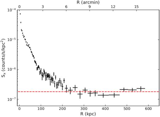
The surface brightness profile of galaxy group 3C 88 in the 0.7–2.0 keV band. The red dashed line represents the surface brightness of the local X-ray background.
Author notes
Einstein and Spitzer Fellow.
