


Abstract
We present a study of the long-term optical variability of young T Tauri stars using previously unpublished data from the Super-Wide Angle Search for Planets (SuperWASP) project. Other publicly available photometry from the Northern Sky Variability Survey (NSVS) and the National Aeronautics and Space Administration (NASA) K2 mission were used to check and supplement our results. Our sample includes 20 weak-lined T Tauri stars in the Taurus–Auriga star-forming region. We have performed a period search on the long time-series photometry and derived the mean periods of stars in our sample. We have found new periods for the stars V1334 Tau (HD 283782) and V1349 Tau (HD 31281), which are without any period estimation in the literature. The rotation period was found for the primary star in the binary V773 Tau (HD 283447). Several earlier results were updated. For the star V410 Tau (HD 283518), we have compared the light-curve changes found in previous studies with the new measurements and attributed the evolution of spots to a ∼15-year cycle similar to the solar 11-year cycle. We have also derived luminosities and effective temperatures for our targets, in order to locate them in the Hertzsprung–Russell diagram and calibrate the masses and ages of the target stars.
1 INTRODUCTION
The kinematic association of many T Tauri stars with dark clouds where stars are formed (Herbig 1977) and the presence of Li i λ6707 Å in absorption (Bertout 1989) show that T Tauri stars are young stellar objects. They have low or intermediate masses (0.5–2.5 M⊙) and are defined as pre-main-sequence (PMS) stars that are surrounded by a nebula and show emission lines in their spectra (Joy 1945). These objects typically have spectral types ranging from G to M. PMS models show that their interiors are either fully convective or possess outer convective envelopes, depending on the age and mass of the star (Hussain 2012). The properties of these PMS objects were reviewed by e.g. Menard & Bertout (1999), who emphasized two subgroups: the so-called ‘classical’ T Tauri stars (CTTS), still actively accreting from their circumstellar discs, and the ‘weak-line’ T Tauri stars (WTTS), no longer surrounded by a circumstellar disc.
Depending on their spectral type, T Tauri stars can have ages ranging from less than one to tens of Myr. Comparing the position of these stars in the Hertzsprung–Russell (HR) diagram with theoretical evolutionary tracks (D’Antona & Mazitelli 1994; Swenson et al. 1994) gives an upper limit on the estimated age of the stars. However, these evolutionary tracks do not take into account accretion and Siess, Forestini & Bertout (1997) show that they underestimate ages by a factor of 2–3.
Ubiquitous amongst T Tauri stars is their variability. As was already noticed in the original definition by Joy (1945), the prototype T Tauri exhibits strong and mostly irregular variability on time-scales from hours to months and even years. This is true for broad-band photometry at all wavelengths (radio to X-ray). On top of a periodic signal due to star spots, modulated by stellar rotation, the reason for this type of variability is stellar youth, apparent through strong magnetic activity and variable accretion and/or extinction (Herbst et al. 1994). Variations are not restricted to photometric observations. Emission lines are also changing in intensity and shape (e.g. Johns & Basri 1995; Lago & Gameiro 1998) and polarimetric studies imply variations in the degree and position angle of polarization as well (Appenzeller & Mundt 1989).
There have been many previous photometric surveys in the optical and infrared. We refrain from presenting a comprehensive overview here, but mention several surveys that have studied the photometric variability of our target stars. Bouvier et al. (1997) observed in the optical range 58 WTTS that were detected in the ROSAT All-Sky Survey (RASS). They were able to derive rotational periods for 18 of their stars, all but one being ascribed to rotational modulation by stellar spots. Grankin et al. (2008) presented a homogeneous set of photometric measurements for WTTS extending for up to 20 years. Their data were collected within the framework of the Research Of Traces Of Rotation (ROTOR) programme, aimed at the study of the photometric variability of PMS objects. The data set contains rotational periods for 35 out of 48 stars. Further optical photometry, including the behaviour on time-scales over more than several years, has been studied in the works of Gahm et al. (1993), Grankin et al. (2007), Percy et al. (2010) and Ibryamov, Semkov & Peneva (2015).
Recently, Rigon et al. (2017) presented a study, including long-term variability of CTTS (mostly in the Taurus–Auriga region), based on data from the Wide Angle Search for Planets (SuperWASP). They found that the overwhelming majority of CTTS have a low-level variability with σ < 0.3 mag, dominated by time-scales of a few weeks, consistent with rotational modulation. The presence of long-term variability correlates with the spectral slope at 3–5 |$\mu$|m, which is an indicator of inner disc geometry, and with the U − B band slope, which is an accretion diagnostic. This shows that long-term variations in CTTS are driven predominantly by processes in the inner disc and accretion zone.
The extensive simultaneous multiwavelength studies of Carpenter, Hillenbrand & Skrutskie (2001) find that the bulk of T Tauri stars show photometric variability of the order of 0.2 mag in JHKs and ∼0.5 mag in their respective near-infrared (NIR) colours. Further characterization in the NIR was studied by e.g. Eiroa et al. (2002), Alves de Oliveira & Casali (2008) and Rice, Wolk & Aspin (2012). The photometric properties have been extended to the mid-infrared (Flaherty et al. 2012; Rebull et al. 2010) and to the far-infrared (Billot et al. 2012).
The most advanced survey of T Tauri stars to date is the Coordinated Synoptic Investigation’s study of the NGC 2264 star-forming region (CSI 2264: Cody et al. 2014). The multi-wavelength observation campaign utilized 16 telescopes, including the space-based observatories CoRoT and Spitzer. Their unprecedented photometric precision of |$\le\!1{{\ \rm per\ cent}}$| and a cadence down to several minutes sets a new standard for this kind of survey. Cody et al. (2014), McGinnis et al. (2015) and Stauffer et al. (2015) show that young-star variability can be caused not only by cold spots but also by circumstellar obscuration events, hot spots on the star and/or disc, accretion bursts and rapid structural changes in the inner disc.
The main goal of our study is to extend knowledge of T Tauri stars by analysing several years of high-cadence monitoring of 20 WTTS using data from the SuperWASP (Street et al. 2003) and Northern Sky Variability Survey (NSVS) survey (Woźniak et al. 2004). Our particular emphasis is to search for possible evolution in the long-term variability of brightness changes caused by the presence of spots.
2 TARGET SELECTION
We have found that many bona fide T Tauri stars (originally designated as members of the Tau–Aur region) in publications listed in Table 1 are without reliable periods of photometric variability and/or physical parameters. We excluded any known CTTS and stars with close visual companions from the list. Furthermore, we selected only stars with V < 11 mag, as this is the brightness limit for spectroscopic follow-up observations at Stará Lesná observatory (Pribulla et al. 2015). We arrived at a sample of 20 WTTS. All the targets have been observed by our own spectroscopic survey and the equivalent width (EW) of the Li λ6707 line was measured to confirm the evolutionary status of the targets. Patterer et al. (1993) found, for HD 283518 (V410 Tau), EW(Li) = 0.547 ± 0.084 Å. All other stars in our sample had their EWs measured in the range of 0.165–0.472 Å.
| Object | SuperWASP ID | R.A. | Dec. | Vmag | Sp. type | P [d] | Dist. [pc] | Refer. |
|---|---|---|---|---|---|---|---|---|
| NSVS ID | (2000) | (2000) | ||||||
| HD 285281 | 1SWASPJ040031.06+193520.8 | 04 00 31.07 | 19 35 20.8 | 10.17 | K1 | 1.1683 | 135.3|$^{+1.2}_{-1.2}$| | (1)(2)(6) |
| 9414189? | ||||||||
| BD+19 656 | 1SWASPJ040519.59+200925.5 | 04 05 19.61 | 20 09 25.2 | 10.12 | K1 | 2.86 | 108.5|$^{+0.7}_{-0.7}$| | (2)(3)(6) |
| 9417695? | (0.741) | |||||||
| HD 284135 | 1SWASPJ040540.58+224812.0 | 04 05 40.58 | 22 48 12.0 | 09.39 | G3V | 0.8160 | – | (1)(6) |
| 6750588 | ||||||||
| HD 284149 | 1SWASPJ040638.08+201811.1 | 04 06 38.80 | 20 18 11.2 | 09.63 | G0 | 1.0790 | 118.2|$^{+0.7}_{-0.7}$| | (1)(2)(4)(6) |
| 9418722 | ||||||||
| HD 281691 | 1SWASPJ040909.74+290130.2 | 04 09 09.74 | 29 01 30.3 | 10.68 | G8III | 2.74? | 110.3|$^{+0.5}_{-0.5}$| | (1)(6) |
| 6754307 | ||||||||
| HD 284266 | 1SWASPJ041522.91+204417.0 | 04 15 22.92 | 20 44 16.9 | 10.51 | K0V | 1.83 | 119.9|$^{+1.0}_{-1.0}$| | (1)(2)(6) |
| 9425183 | ||||||||
| HD 284503 | 1SWASPJ043049.18+211410.6 | 04 30 49.19 | 21 14 10.7 | 10.24 | G8 | 0.736 | 111.6|$^{+0.7}_{-0.7}$| | (1)(6) |
| 9436598 | ||||||||
| HD 284496 | 1SWASPJ043116.85+215025.2 | 04 31 16.86 | 21 50 25.3 | 10.80 | K0 | 2.71 | 125.8|$^{+0.6}_{-0.6}$| | (1)(5) |
| 9444066? | ||||||||
| HD 285840 | 1SWASPJ043242.43+185510.2 | 04 32 42.43 | 18 55 10.2 | 10.85 | K1V | 1.55 | 90.5|$^{+0.3}_{-0.3}$| | (2)(5)(6) |
| 9444857? | ||||||||
| HD 285957 | 1SWASPJ043839.06+154613.6 | 04 38 39.07 | 15 46 13.6 | 10.86 | K1 | 3.07 | 139.2|$^{+1.1}_{-1.1}$| | (2)(5)(6) |
| 9449108 | ||||||||
| HD 283798 | 1SWASPJ044155.15+265849.4 | 04 41 55.16 | 26 58 49.4 | 09.55 | G7 | 0.6? | 110.8|$^{+0.6}_{-0.6}$| | (1)(2)(6) |
| 6778011 | ||||||||
| HD 283782 | 1SWASPJ044454.45+271745.2 | 04 44 54.40 | 27 17 45.5 | 09.48 | K1 | ? | 168.0|$^{+6.8}_{-6.3}$| | (1)(2)(6) |
| 6780256 | ||||||||
| HD 30171 | 1SWASPJ044551.29+155549.7 | 04 45 51.30 | 15 55 49.7 | 09.36 | G5 | 1.104 | 184.9|$^{+3.9}_{-3.7}$| | (2)(5)(6) |
| 9455701 | ||||||||
| HD 31281 | 1SWASPJ045509.62+182631.1 | 04 55 09.62 | 18 26 31.1 | 09.14 | G1 | ? | 122.4|$^{+0.6}_{-0.6}$| | (1)(2)(6) |
| no data | ||||||||
| HD 286179 | 1SWASPJ045700.64+151753.1 | 04 57 00.65 | 15 17 53.1 | 10.39 | G3 | 3.33 | 123.7|$^{+1.0}_{-1.0}$| | (5)(6) |
| 9466913 | ||||||||
| HD 286178 | 1SWASPJ045717.65+152509.4 | 04 57 17.66 | 15 25 09.5 | 10.54 | K1 | 2.39 | 74.3|$^{+3.5}_{-3.2}$| | (2)(5)(6) |
| 9467195 | ||||||||
| HD 283447 | 1SWASPJ041412.91+281212.3 | 04 14 12.92 | 28 12 12.3 | 10.68 | K3V | 51 | 128.1|$^{+2.3}_{-2.3}$| | (8) |
| 6758228 | ||||||||
| HD 283572 | 1SWASPJ042158.84+281806.4 | 04 21 58.85 | 28 18 06.5 | 09.03 | G5 | 1.529 | 130.3|$^{+0.9}_{-0.9}$| | (1)(2) |
| no data | ||||||||
| HD 285778 | 1SWASPJ042710.57+175042.6 | 04 27 10.57 | 17 50 42.6 | 10.22 | K1 | 2.734 | 120.1|$^{+0.8}_{-0.8}$| | (7) |
| 9440985 | ||||||||
| HD 283518 | 1SWASPJ041831.10+282716.0 | 04 18 31.12 | 28 27 16.1 | 10.75 | K3V | 1.87 | 130.4|$^{+0.9}_{-0.9}$| | (1)(9)(10) |
| 6761377 |
2.1 Evolution stage of target stars
For analysis of the evolutionary status of a star, the effective temperature and luminosity are needed to locate the object in the Hertzsprung–Russell diagram (HRD). Then the age and mass can be deduced from the corresponding isochrones.
Only stars with an available parallax from the Gaia DR2 (Lindegren et al. 2018) or earlier Tycho–Gaia Astrometric Solution (TGAS) catalogue (Michalik, Lindegren & Hobbs 2015) were included in this analysis. We have used parallax from TGAS only for HD 286178, since the value is missing in the newer Gaia DR2 catalogue. However, based on its distance, HD 286178 may not be a member of the Taurus–Auriga SFR. For HD 283782, the Gaia DR2 found two astrometric positions separated by only 1.9 arcsec. We have used the parallax of the brighter (in the Gaia G band) target, closer to RA2000, Dec2000 of HD 283782. No parallax was available for star HD 284135. The calculation of luminosity is based on the parallax (or distance), apparent magnitude, reddening and bolometric correction (BC). Within the Gaia and Hipparcos eras, we now have quite accurate parallaxes for stars in the solar vicinity, where our targets are also located. The estimation of reddening, especially in denser areas such as the Taurus–Auriga region, still poses several problems and limitations. One way out of the dilemma could be reddening maps (Schlafly et al. 2014). However, their resolution is not sufficient for our purpose. We therefore used another approach, by taking available reddening estimates from the literature (Meištas & Straišys 1981; Chavarría-K et al. 2000; Grankin 2013; Herczeg & Hillenbrand 2014) and the dereddening method based on the Strömgren–Crawford uvbyβ photometric system (Crawford 1975; Schuster & Nissen 1989). The uvbyβ photometric data were taken from Paunzen (2015). An unweighted mean and its error in AV were calculated (Table 2). The values for AV range up to 1.10 mag, with a mean of the error of 0.13 mag. These values agree with that expected in this region of the sky. However, the uncertainties are the largest contribution to the overall error in log L/L⊙. The BC, especially derived for PMS stars, were taken from Pecaut & Mamajek (2014).
The astrophysical parameters of our targets with available parallax measurements.
| Object | AV | log Teff | BCV | log L/L⊙ | M [M⊙] | age [Myr] |
|---|---|---|---|---|---|---|
| HD 285281 | 0.47(2) | 3.699(22) | −0.27 | +0.43(1) | 1.4–1.7 | 1–8 |
| BD+19 656 | 0.27(4) | 3.703(9) | −0.26 | +0.07(2) | 1.2–1.3 | 7–12 |
| HD 284149 | 0.19(18) | 3.775(11) | −0.04 | +0.28(5) | 1.0–1.2 | 15–25 |
| HD 281691 | 0.19(11) | 3.703(9) | −0.26 | −0.01(4) | 1.1–1.3 | 8–18 |
| HD 284266 | 0.16(23) | 3.724(20) | −0.18 | −0.01(9) | 1.0–1.2 | 15–30 |
| HD 284503 | 0.19(5) | 3.720(17) | −0.19 | +0.05(2) | 1.1–1.3 | 10–20 |
| HD 284496 | 0.21(7) | 3.716(13) | −0.21 | +0.00(3) | 1.1–1.2 | 12–20 |
| HD 285840 | 0.17(25) | 3.720(25) | −0.19 | −0.33(10) | 0.8–1.0 | 20–70 |
| HD 285957 | 0.27(33) | 3.695(13) | −0.29 | +0.12(13) | 1.2–1.5 | 3–13 |
| HD 283798 | 0.00(1) | 3.756(8) | −0.09 | +0.19(1) | 0.9–1.3 | 17–21 |
| HD 283782 | 0.63(19) | 3.716(29) | −0.21 | +0.96(18) | 1.8–2.7 | <3 |
| HD 30171 | 0.36(13) | 3.736(16) | −0.15 | +0.91(6) | 2.1–2.5 | 2–4 |
| HD 31281 | 0.26(13) | 3.763(7) | −0.06 | +0.54(5) | 1.4–1.6 | 8–12 |
| HD 286179 | 0.44(29) | 3.756(15) | −0.09 | +0.19(12) | 1.1–1.4 | 10–35 |
| HD 283447 | 0.95(10) | 3.690(13) | −0.30 | +0.36(4) | 1.4–1.7 | 2–4 |
| HD 283518 | 1.10(10) | 3.643(44) | −0.60 | +0.53(4) | 0.5–1.6 | <2 |
| HD 283572 | 0.48(3) | 3.740(24) | −0.14 | +0.82(1) | 1.8–2.5 | 2–5 |
| HD 285778 | 0.15(11) | 3.720(12) | −0.19 | +0.14(4) | 1.2–1.4 | 8–15 |
The apparent magnitudes are from Grankin (2013), except for HD 30171, HD 283447, HD 283798 and HD 283518, which are not included in this reference. For these stars, we have used values from the AAVSO Photometric All-Sky Survey (APASS), after checking the magnitudes in common with Grankin (2013), which yielded an excellent agreement. For the final error estimation in log L/L⊙, we applied full propagation of uncertainties for all the measurements.
A careful assessment of the literature regarding the effective temperature estimation of T Tauri stars revealed that there are significant differences in the values for individual stars. These are caused by the usage of different stellar atmospheres, spectral resolution, analytic methods and so on. An excellent example of the challenges to be faced is shown by Lebzelter et al. (2012) for the case of cool-type giants. As for reddening, no homogeneous source was found. We therefore calculated unweighted means of values from the literature (Palla & Stahler 2002; Ammons et al. 2006; Wright et al. 2011; Grankin 2013; Davies, Gregory & Greaves 2014; McDonald, Zijlstra & Watson 2017) and the Strömgren–Crawford uvbyβ calibration of Napiwotzki, Schoenberner & Wenske (1993). The latter is based on the β index, which is an excellent indicator for log Teff. The combination of a narrow and wide filter centred at Hβ guarantees that any possible emission has no significant effect. The final uncertainties are between 100 and 450 K, respectively. In Table 2, all the derived astrophysical parameters with their uncertainties are listed.
Finally, we used PMS evolutionary tracks based on the Pisa stellar models (Tognelli, Prada Moroni & Degl’Innocenti 2011) to investigate the evolutionary status of our targets. Evolutionary tracks with [X, Y, Z] of [0.609, 0.2533, 0.1377], i.e. solar metallicity, were used. In Fig. 1, the location of the target stars in the log Teff versus log L/L⊙ diagram is shown. The error bars were used to determine the extent of the possible masses and ages (also in Table 2) of candidate stars in comparison with Pisa stellar model isochrones. We have found that the stars in our sample should be younger than 70 Myr at most. This is close to, or inclusive of, the 10–100 Myr interval for post T Tauri stars (PTTS) defined by Jensen (2001). The uncertainties, due mainly to effective temperature, allow for the estimation of masses to within the range ±0.1 M⊙ to ±0.2 M⊙. To make a comprehensive analysis of the correlation between the rotational period and evolutionary status of our targets, more precise and homogeneous effective temperatures are required.
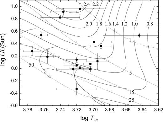
Location of the target stars in the log Teff versus log L/L⊙ diagram, together with the PMS evolutionary tracks (solid curves) and isochrones (dotted curves) based on the Pisa stellar models (Tognelli et al. 2011). The evolutionary tracks range from 2.4–0.8 M⊙ and isochrones from 1–50 Myr, as indicated.
3 PHOTOMETRIC DATA
For the determination of periods, we needed light curves measured during long observation campaigns, which are best taken with the same instrument and reduced with the same pipeline. There are several public data available, notably the SuperWASP data base. With our access to all of the data presently kept in the SuperWASP archives, we have based our photometric light-curve investigation on almost 8 years of observations. The separation into observing seasons is a natural one, since the target region was best observable from autumn to spring. To expand our time domain, we have also added photometry from the NSVS archive. For 10 targets, we have found photometry provided by the Kepler K2 mission. We break down the individual observing seasons in Table 3.
Observing season break-up for the NSVS (≡0) and SuperWASP data. Not all of the target stars were observed in all seasons. When using the whole data set, we refer to the one named Σ. Additional observations by the K2 Mission were used as C4 and C13.
| Season | Start | End | Dur. [d] |
|---|---|---|---|
| 0 | 1999-08-06 | 2000-03-26 | 233 |
| 1 | 2004-07-29 | 2004-09-30 | 63 |
| 2 | 2006-09-17 | 2007-02-27 | 163 |
| 3 | 2008-01-25 | 2008-02-06 | 12 |
| 4 | 2008-10-13 | 2009-03-07 | 145 |
| 5 | 2009-08-12 | 2010-03-26 | 226 |
| 6 | 2010-08-27 | 2011-02-16 | 173 |
| 7 | 2011-09-24 | 2012-01-30 | 128 |
| Σ | 1999-08-06 | 2012-01-30 | 4560 |
| C4 | 2015-02-08 | 2015-04-20 | 70 |
| C13 | 2017-03-08 | 2017-05-27 | 80 |
3.1 SuperWASP data
The WASP instruments have been described by Pollacco et al. (2006) and the reduction techniques discussed by Smalley et al. (2011) and Holdsworth et al. (2014). The aperture-extracted photometry from each camera on each night was corrected for atmospheric extinction, instrumental colour response and system zero-point relative to a network of local secondary standards. The resulting pseudo-V magnitudes are comparable with Tycho-2 (Høg et al. 2000) V magnitudes (Butters et al. 2010). In this article, we have used SuperWASP data that are so far unavailable publicly, provided by our co-author B. Smalley.
The SuperWASP data were gathered from 2004 July–2012 January, covering seven observing seasons in total. The mean season duration is 143 days; however, season 3 consists of only 12 days. Usually we had five different seasons available for our targets. For the star HD 31281, we found only two seasons of useful data in the archive. The mean cadence of observations is ∼80 s.
For all targets, the SuperWASP archive provides 417 603 points in total and typically ∼4000 points per object in each season. The SuperWASP pre-clean procedure includes the following steps: (i) keeping data with errors < 0.2 mag, (ii) finding the median and (iii) keeping data within a brightness interval ±0.2 mag from the median. This procedure reduced our data set by only 2.4 per cent.
3.2 NSVS data
The Northern Sky Variability Survey (NSVS) is a temporal record of the sky over the optical magnitude range from 8–15.5. It was conducted by the first-generation Robotic Optical Transient Search Experiment (ROTSE-I), using a robotic system of four co-mounted unfiltered telephoto lenses equipped with CCD cameras. The survey was conducted from Los Alamos, New Mexico and primarily covers the entire northern sky (Woźniak et al. 2004). The NSVS contains light curves for approximately 14 million objects with a 1-yr baseline and typically 100–500 measurements per object. The NSVS public data release is available through a dedicated web page.1
We refer to the NSVS data as ‘Season 0’ (in Tables 3 and 4). We have to note that, for HD 31281 and HD 283572, no NSVS data are available. The mean cadence of observations of NSVS data was only ∼0.6 d. Because of the few data points (∼105 per star) and the fact that the NSVS data usually only observed a single point per night, we have opted to not remove any of them.
Results of period analysis for all target objects. The prominent periods for the same object are listed by decreasing power. Seasons without any usable data are marked as ‘–’. The last column lists periods obtained from the literature (see Table 1). ‘?’ denotes uncertain values. Values in brackets ‘〈’, ‘〉’ are not considered as the intrinsic period.
| Object | Most prominent period [d] in seasons | Pmean [d] | Amean [mag] | Plit [d] | |||||||
|---|---|---|---|---|---|---|---|---|---|---|---|
| 0 | 1 | 2 | 3 | 4 | 5 | 6 | 7 | Σ | |||
| HD 285281 | 1.1697(37) | 1.1689(29) | 1.1705(39) | – | – | 1.1706(44) | 1.1722(36) | 1.1716(12) | 1.1711(37) | 0.0413(51) | 1.1683 |
| BD+19 656 | 〈1.0041(285)〉 | 〈1.4421(207)〉 | 2.9104(353) | – | – | 2.8885(59) | 2.8869(289) | 〈1.4611(188)〉 | 2.8849(51) | 0.0080(3) | 2.8600 |
| 〈0.7410〉 | |||||||||||
| HD 284135 | 〈0.9986(204)〉 | 0.8181(144) | 0.8183(69) | – | – | 0.8175(325) | 0.9175(121) | 0.8245(67) | 0.8179(58) | 0.0106(20) | 0.8160 |
| HD 284149 | 1.0309(316) | 1.0353(192) | 1.0534(224) | – | – | 1.0473(268) | 1.0419(362) | 1.0684(84) | 1.0712(7) | 0.0084(3) | 1.0790 |
| HD 281691 | 2.6596(171) | 2.6511(77) | 2.6610(294) | – | – | 2.6274(339) | 2.6589(328) | 2.6226(157) | 2.6267(237) | 0.0177(17) | 2.74? |
| HD 284266 | 1.8086(185) | 1.8218(237) | 1.8087(183) | – | – | 〈0.9016(133)〉 | 1.8396(24) | 1.8403(88) | 1.8433(10) | 0.0315(4) | 1.83 |
| HD 284503 | 0.5166(183) | 0.7396(148) | 0.7369(227) | – | – | 0.7308(78) | 0.7363(64) | 0.7369(58) | 0.7370(3) | 0.0267(25) | 0.736 |
| HD 284496 | 2.7248(211) | 2.7056(205) | 2.7390(336) | – | – | 2.6617(266) | 2.7556(882) | 2.6846(763) | 2.6880(195) | 0.0486(23) | 2.71 |
| HD 285840 | 1.5562(177) | – | 〈1.2241(3247)〉 | 1.5323(1134) | – | 1.5470(395) | 1.5751(306) | 1.5538(224) | 1.5476(67) | 0.0315(26) | 1.55 |
| HD 285957 | 3.0874(294) | – | 3.0497(330) | 〈4.1736(5446)〉 | 3.0798(236) | 3.0950(534) | 3.0619(383) | 3.0931(336) | 3.0546(255) | 0.0251(15) | 3.07 |
| HD 283798 | 0.9868(107) | 〈0.8906(1934)〉 | 0.9861(92) | – | – | 〈0.9957(340)〉 | 0.9890(154) | 0.9860(93) | 0.9872(33) | 0.0159(5) | 0.6? |
| HD 283782 | 〈1.0016(91)〉 | 〈1.0413(319)〉 | 〈0.8706(1873)〉 | – | – | 〈1.0589(872)〉 | 〈0.8716(1333)〉 | 〈0.8684(1139)〉 | 〈0.8704(1106)〉 | 0.0081(26) | ? |
| HD 30171 | 〈0.9956(2272)〉 | – | 1.1053(873) | 1.1013(1057) | 1.1106(141) | 1.1055(210) | 1.1101(141) | 1.1062(164) | 1.1058(33) | 0.0272(13) | 1.104 |
| 〈0.5254(32)〉 | |||||||||||
| HD 31281 | – | – | 〈0.7920(1100)〉 | 〈0.7960(1181)〉 | – | – | – | – | 〈0.7913(15)〉 | 0.0098(12) | ? |
| HD 286179 | 3.2573(627) | – | 3.1486(1914) | 〈0.9272(621)〉 | 3.1260(401) | 3.1476(501) | 3.3201(199) | – | 3.1397(221) | 0.0294(13) | 3.33 |
| HD 286178 | 〈0.7490(15)〉 | – | 〈1.6958(281)〉 | 〈0.7759(1023)〉 | 2.3680(399) | 〈1.6981(329)〉 | 〈1.6990(387)〉 | – | 〈1.7001(81)〉 | 0.0231(37) | 2.39 |
| 2.0442(125) | 2.4242(551) | 2.0198(210) | 〈1.7013(220)〉 | 2.4155(642) | 2.4155(735) | 2.4125(164) | 0.0227(34) | ||||
| HD 283447 | 3.0883(239) | 3.0741(1071) | 3.0912(268) | – | – | 3.0628(141) | – | 3.0826(374) | 3.0836(210) | 0.0695(24) | 51 |
| HD 283572 | – | 1.5392(175) | 1.5475(227) | – | – | 〈1.4077(829)〉 | 1.5823(544) | 1.5470(208) | 1.5462(38) | 0.0386(22) | 1.529 |
| HD 285778 | 〈0.9951(333)〉 | – | 〈1.2602(194)〉 | 〈0.9801(879)〉 | 2.7293(1542) | 2.7412(541) | 2.7360(1030) | 2.7308(759) | 2.7361(204) | 0.0132(32) | 2.734 |
| HD 283518 | 1.8723(26) | 1.8716(63) | 1.8713(645) | – | – | 1.8734(641) | 〈0.9361(118)〉 | 1.8702(377) | 1.8706(14) | 0.0491(18) | 1.87 |
| 〈0.9362(27)〉 | 〈0.9358(35)〉 | 〈0.9356(151)〉 | 〈0.9367(239)〉 | 〈0.9351(92)〉 | |||||||
Note. Uncertain periods are discussed further in Section 4.3.
To be able to analyse the NSVS data together with the SuperWASP data, we have made a simple linear transformation in magnitude. For each target star, we have found the mean magnitude (mS) from the whole pre-cleaned SuperWASP data set. Then we have computed the mean magnitude (mN) of the corresponding NSVS data set. All the NSVS data were shifted by mN − mS. We are interested mainly in the temporal positions of extremes in the light curves and the possible scaling of the amplitude of the NSVS light curve is of little concern.
3.3 Kepler K2 data
The Keplermission was launched on 2009 March 6. Although it was designed primarily to detect variable stars and find transiting exoplanets (Borucki et al. 2010), the mission also provided exceptionally high photometric performance for all stars inside its field of view (FOV). The original FOV was centred in the constellation Cygnus (Koch et al. 2010). After pointing and stability problems, the mission was extended to other fields along the ecliptic and dubbed K2 (Howell et al. 2014). The estimated photometric precision is down to 400 ppm for stars with V = 12 mag (Howell et al. 2014). In the original proposal, the Taurus–Auriga cluster was planned for the C4 (2015 February–April, centred at RA = 03 56 18, Dec. = +18 39 38) observational campaign. After the next extension, another field C13 (2017 March–May, centred at RA = 04 51 11, Dec. = +20 47 11) was added.2
Since we were unable to find reliable periods in some observational seasons for several targets, we wanted to confirm and refine the values using the Kepler data. With the exception of TTS20, we have only one season of data per target available. The data were observed with a 30-min exposure in the Kepler magnitude (white light). Since we were interested in periods longer than 0.2 days, we have used the provided PDC SAP flux, corrected directly for most systematics by the data conditioning pipeline (Stumpe et al. 2012).
Because we have used Kepler data in a separate analysis, we did not need to transform the measured fluxes or the Kepler magnitudes.
4 PERIOD SEARCH
The majority (70 per cent of observation nights) of all photometric data were provided from the SuperWASP archive (seasons 1–7) with a mean cadence of 80 seconds. We have also added ground-based data from the NSVS (season 0) with a mean cadence over the whole data set of 0.6 days. However, if there was more than one data point per observation night, the mean cadence was about 45 min. 10 out of the 20 targets were observed in campaign fields of the K2mission with a 30-min long cadence. All of the chosen data sets are usable for period searches in the regime of several days. Although the NSVS data set has the lowest cadence, it has the longest duration of a single season (see Table 3). The previously identified rotational periods were in the range of 0.7–3.33 days (Table 1).
We chose to investigate the individual observing seasons separately to account for possible period changes between them. The problematic season 3 (with only 12 nights of observations) and season 4 (usually with very few data) were investigated only when non-trivial Fourier plots were found. Finally, we have also performed a period search on the combined data set (Σ), constituted from seasons 0–7. The NSVS data were transformed before adding them into the combined data set (see Section 3.2). The phased light curves presented in Figs S4 and S5 were constructed using all available ground-based pre-cleaned data points (see Section 3.1) and folded on the period corresponding to the most prominent frequency found in the Σ data set.
Kepler data sets (seasons C4 and C13) were investigated separately from the ground-based data. Except for star HD 285778, only one season of K2 data was available per object. In the single special case, we have conducted the period search on both C4 and C13 data separately.
4.1 Ground-based data
The period analysis was performed using the date-compensated discrete Fourier transform algorithm (DC DFT) of Ferraz-Mello (1981). The advantage of this method is that it compensates for gaps within the data set using weighting, alias discrimination and harmonic frequency filtering.
The starting frequency was chosen based on the length of the combined data set to be 0.00011 cycle day–1. This corresponds roughly to periods between 0.2 and 9000 days. The step in frequency was set to an average of 0.0001 cycle day–1. Because the NSVS data provided only a handful of points per night, we have set our maximum frequency to 2 cycle day–1 and all Fourier plots (Figs S1 and S2) are calculated up to this frequency.
We have used two software packages that utilize DC DFT to search for periods in our data sets.
The initial analysis was done with the vstar package developed by the American Association of Variable Star Observers (AAVSO). This tool allowed us to search for all significant periods (intrinsic or harmonic) and order them with decreasing power in their Fourier spectrum. It also enabled visual checks to affirm the periodicity by constructing phase plots for any given frequency (period).
A subsequent analysis was done using the period04 software (Lenz & Breger 2004) with the same frequency range and frequency step for DC DFT. The code searches only for the most prominent frequency in the Fourier spectrum. The list of suspected frequencies (periods) from previous investigations using the vstar package was refined using period04. The advantage of period04was that noise peaks were less likely to be included in the final list of identified frequencies (Breger et al. 2011).
To further discern the intrinsic periods from aliases, we have constructed the spectral window of each data set (e.g. see Fig. 2). The most significant period peak was convolved with the spectral window and subtracted from the previously computed period spectrum (i.e. the corresponding frequency was pre-whitened for the next analysis).
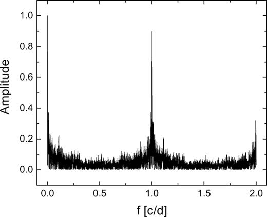
The spectral window of the SuperWASP data set (Σ) constructed for HD 285957. This target has the most observation nights available.
The result was inspected visually. If the root mean square (RMS) of the residuals was too large, the peak was discarded from the subsequent analysis. Frequency peaks with a signal-to-noise ratio >2.0 were considered for further analysis. The procedure was repeated until the amplitude of the most significant peak left was |$\le 10{{\ \rm per\ cent}}$| of the original most significant period. Remaining frequencies were included in Table 4.
After periodicity was identified, we performed a Marquardt-algorithm-based non-linear least-squares fitting (Bevington & Robinson 1993) simultaneously with all the identified frequencies, resulting in an adjusted set of parameters (i.e. frequencies, amplitudes and phases).
The least-squares fit by period04 also provided an error matrix, but the derived uncertainties only estimate the consistency of the fit. The period04 package has a tool to compute more realistic uncertainties using Monte Carlo simulations, which we have used with the default values.
The detected periodic signals were subtracted out and the remaining data points were rearranged randomly, with the original time stamps preserved. A pseudo-random (based on the onboard computer time) Gaussian noise with a standard deviation of 0.1 was added to the magnitudes predicted by the last fit. For each optimization, a set of total 100 test time strings was generated. The identification of peaks and least-squares fits to the light curve was carried out for each of the simulated time strings. The uncertainties were calculated using the distribution of fit parameters (Lenz & Breger 2005).
4.2 Kepler data
The period analysis was performed separately from the ground-based data. However, the same frequency domain (0.00011–2 cycle day–1) was searched with a step of Δf = 0.0001 cycle day–1. The mean data error was only 26 ppm. Combined with the 30-min cadence and almost uninterrupted 70–80 days of observation, the resulting Fourier plots (Fig. S3) are without much noise and period peaks are easily distinguishable. The peaks of the most significant periods in the regime of several days correspond to intrinsic changes of brightness and no spectral window aliases were expected above a frequency of ∼1/80 = 0.0125 cycle day–1.
The resulting most significant periods are presented in Table 5. We have compared the periods found from the Kepler data with the mean periods found in our previous analysis of SuperWASP and NSVS data, as well as with the values found in the literature.
Results of period analysis for objects with available Kepler data. Periods, PKepler, are ordered by decreasing power of the corresponding peak. Values in brackets ‘〈’, ‘〉’ are not considered as the intrinsic period. Comparisons with previously determined periods (Plit) and periods based on SuperWASP data (Pmean) are also shown.
| Object | Plit [d] | Pmean [d] | PKepler [d] | Field |
|---|---|---|---|---|
| BD+19 656 | 2.86 | 2.8849(51) | 2.8489(8) | C4 |
| 〈1.4467(4)〉* | ||||
| HD 284496 | 2.71 | 2.6880(195) | 2.7738(8) | C13 |
| 〈2.6525(6)〉 | ||||
| HD 285840 | 1.55 | 1.5476(67) | 1.5463(2) | C13 |
| 〈0.7735(1)〉* | ||||
| HD 285957 | 3.07 | 3.0546(255) | 3.0863(10) | C13 |
| 〈1.5311(2)〉* | ||||
| HD 283798 | 0.6? | 0.9872(33) | 0.9831(2) | C13 |
| 〈0.9658(2)〉 | ||||
| HD 283782 | ? | 〈0.8704(1106)〉 | 2.0181(4) | C13 |
| HD 31281 | ? | 〈0.7913(15)〉 | 0.6771(1) | C13 |
| 〈0.7999(1)〉 | ||||
| HD 286179 | 3.33 | 3.1397(221) | 3.1249(20) | C13 |
| 〈1.5647(5)〉* | ||||
| HD 286178 | 2.39 | 1.7001(81) | 1.7027(6) | C13 |
| 〈2.3562(11)〉* | ||||
| 〈1.1813(3)〉! | ||||
| HD 285778 | 2.734 | 2.7361(204) | 2.8554(17) | C4 |
| 〈1.3717(4)〉* | ||||
| 2.7510(15) | C13 |
Note. Periods marked with ‘*’ are close to a 1:2 ratio with the more prominent period. See the discussion in text for details on special cases marked with ‘!’.
The period analysis of Kepler data yielded similar periods to those obtained from the ground-based data only. The mean difference was of the order of ∼0.1 days. In comparison with Table 4, the mean uncertainties in period were smaller because of clear and prominent peaks in Fourier plots. Several dubious periods (e.g. for BD+19 656) found in some observing seasons in SuperWASP data were also discovered with smaller amplitudes and corresponded to a near 1:2 period ratio with the most prominent period. This indicates that spot areas are distributed along the length of the equator. For stars HD 283782 and HD 31281, we were able to find the first reliable periods from the Kepler data only. Objects with different period estimates are discussed further in Section 4.3 below.
In addition to period determination, we have looked at the possible evolution of the period during the ∼80-day long Kepler observation. We have used the wavelet Z-transform (WWZ) algorithm by Foster (1996), provided within the vstarpackage. The algorithm can achieve resolution in both frequency and time for unevenly spaced data. The wavelet was a sinusoidal wave shifted by a constant term. A sliding window of constant width (in time) moved across the data.
The highest weight was applied to the data points closest to the centre of the window. The output was a relation between the signal power (Z value) as a function of time and the frequency. We were interested in tracking the maximum Z value for any given time. The frequency corresponding to the maximum Z value was interpreted as 1/P .
To cover the period range from all investigated targets, we have run the wavelet analysis for periods from 0.5–4.0 days, with the light curve separated into 50 time bins. The step in period was set to ΔP = 0.01 days (half of the cadence interval) and the so-called decay parameter was fixed at the default value 0.001. The maximum Z values for individual time bins were plotted along with the corresponding semi-amplitudes of the light curve (see Fig. S8). Since we had only the total flux in the Kepler passband, we have expressed the amplitude of the light curve only as a ratio and not in magnitudes.
We have also constructed a simple spot model to compute artificial light curves with emerging and disappearing spots. The spherical stellar surface was covered with a 360 × 181 mesh in longitude and latitude. The flux was calculated for each grid point, taking into account the size of the local grid, the presence of spots and visibility for the observer. A linear limb-darkening law was used. Spots were placed at arbitrary longitudes (on the equator) and revolved with the rotation period. The inclination of the stellar rotation axis was zero and rigid rotation was assumed. We were able to set the times of appearance and disappearance of individual spots.
We have generated long (duration >10Prot) light curves for several scenarios and applied both period and wavelet analyses using the vstar package. Results of two different setups are presented in Fig. 3.
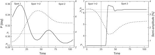
The evolution of period (solid line) and amplitude (dashed line) of the simple spot model light curve. The left panel shows the effect of a new randomly placed spot and subsequent disappearance of the original spot. The right panel shows the effect of two spots placed on opposite sides of the stellar surface, with later disappearance of the original spot.
One typical situation similar to our Sun is when a new spot emerges on the stellar limb while the original spot is still present. After several days, the older spot declines and disappears, while the new one is still present (see the left panel in Fig. 3). The Fourier analysis will find only a ‘median’ period P1 (of periods in the individual spot evolution time step).
If two spotted regions are placed almost on opposite sides of the stellar surface, a sudden change of period is encountered (see the right panel in Fig. 3). Fourier analysis finds two most significant periods (P1, P2). The intrinsic rotation period was closer to the longer period found by Fourier analysis. This means that we have to be cautious about interpreting the most significant periods of Kepler targets. The evolution of rotation period and its amplitude during ∼80 days for all target stars is shown in Fig. S8.
4.3 Discussion on individual targets
The adopted periods we discuss here stem from period analysis of the whole ground-based data set (Σ). We include a note if we have found different non-harmonic periods in a singular observing seasons (see Table 4). Wherever possible, we have preferred the period found in the Kepler data set (Table 5). Fourier plots and wavelet analysis of period evolution can be found in the Supporting Material (Figs S3 and S8).
All periods found for the objects in our sample are interpreted as rotation periods due to magnetic cool spots on the surface of the star. There are other possible sources of periodic signals in T Tauri stars, e.g. hot spots in the circumstellar disc and/or obscuration by material at the inner disc edge. However, studies using the IRAS (Strom et al. 1989) and Spitzer (Padgett et al. 2006) telescopes found that such discs are rare among WTTS. Hartmann et al. (2005) found that, in the Taurus–Auriga region, CTTS are clearly separated from WTTS based on the infrared colour excess. So far, there have been no discs detected around stars in our sample.
For star BD+19 656, we have found two periods in our ground-based data analysed seasonwise. However, the main period was found, when analysing the whole data set and also the K2 data, to be ∼2.85 days, which corresponds to the value previously reported in the literature (see e.g. Grankin 2013). Based on the modelled period evolution, the intrinsic rotation period may be shorter. We have visually examined the Kepler light curve phased with both prominent test periods separately (see Fig. S7) and decided to adopt the period P = 2.8489 days.
Periods of HD 284496 in different observational seasons ranged from ∼2.66 to ∼2.76 days. These two limits were resolved as separate close peaks by the period analysis of Kepler data (see Fig. S3). The most prominent period, P = 2.7738(8) days, was found to be the central value of period changes during the C13 season, investigated by the wavelet analysis. Based on the modelled period evolution, the intrinsic rotation period may be shorter.
For stars HD 285840 and HD 285957, the period analysis of the ground-based and Kepler data provided the same results. The outlier periods found in a single season do not have any physical meaning. Also, the wavelet analysis showed no significant changes (∼0.02 days) over the range of 80 days. The second most significant period found in the K2 data is in a 1:2 ratio to the mean period. This could indicate that some of the larger spotted regions are located on opposite sides of the stellar surface. However, the modelled period evolution showed no sudden change in period. This could be explained by e.g. both spotted regions being present on the surface and small changes of period can be attributed to differential rotation of spots changing their latitude. However, by folding the Kepler light curve with longer and shorter test periods for both stars (see Fig. S7), we have adopted the periods P = 1.5463 days and P = 3.0863 days for HD 285840 and HD 285957, respectively.
The star HD 283798 was found to have a period of P ∼ 0.987 days. However, the corresponding frequency (f = 1.013 cycle day–1) was distinguished from the peak at f = 1.0 (see Fig. S2) and with higher amplitude. This is an unfavourable case for ground-based observations and could be the main reason why the star had no published period in the literature. However, in the K2 data set we have found clear peaks at P = 0.9831(2) and P = 0.9658(2) days.
We have found a previously unpublished period P = 0.87(11) days for HD 283782. However, in several observing seasons we have detected periods close to one day. The Fourier plot (see Fig. S2) was noisy with a mean SNR of 1.7. Because of large uncertainties and spurious periods, we have performed a separate period analysis on the Kepler data. We have found a different prominent peak at P = 2.0181(4) days. The amplitude of the Kepler light curve is only about |$0.25{{\ \rm per\ cent}}$|. Other period peaks were present only in the red-noise region of the Fourier plot (see Fig. S3). We have checked the data distribution in SuperWASP seasons 2, 6 and 7 (i.e. the seasons that yielded the period ∼0.87 day). The mean data cadence was ∼72 s (∼0.0008 day). We have investigated possible harmonic periods from the data sampling in these seasons. The length of uninterrupted observation of the star per night was found to be close to a normal distribution with the centre at ∼4.6 hours (0.192 day). The corresponding frequency is above our threshold, 4.8 cycle day–1. A new period search extended up to 20 cycle day–1 was performed on the whole ground-based data set. Interestingly, a new most prominent period of 0.317 days (3.1545 cycle day–1) was found. The amplitude of frequency corresponding to a period of 0.192 day was less than |$10{{\ \rm per\ cent}}$| of the new most prominent period. We have not been able to link the periods 0.192, 0.317 day, nor their harmonic multiples, to any other period peak found in the Fourier plots for seasons 2, 6 and 7. However, the same period analysis on the K2 data arrived at the most prominent period P = 2.0181(4) days. Based on the modelled period evolution, the intrinsic rotation period may be shorter. We have adopted the Kepler period and consider all estimates from the ground-based data (in Table 4) to suffer from sampling effects. We have found the first reliable period for HD 283782 using the Kepler data set. However, the evolution of this period computed by WWZ shows a decline from the mean by ∼0.2 days accompanied by a small drop in amplitude towards the end of continuous observation. A longer data set would be needed to investigate further. Also, the mean period of 2.02 days also provides problems for ground-based monitoring.
Analysing the data set for HD 31281 is not straightforward, because it was observed only in seasons 2 and 3. The mean cadence was ∼300 seconds spread over only 74 days of observations. This resulted in a high amplitude of the diurnal frequency (f = 1) and the red-noise contribution was also substantial. The intrinsic frequency was found only as the third most significant one (see peaks marked with circles in Fig. S2). Two of the most significant periods were pre-whitened, leaving us with P ∼ 0.79 day from the analysis of all data. The amplitude found was also small, ∼0.01 mag, which is probably the reason no period has been published so far for this object. Fortunately, the K2 data provided a mean period P = 0.6771(1) day. The WWZ analysis showed two distinct periods present over the course of 80 days. A higher period (∼0.8 day) was present for about a quarter of the time interval. This corresponds to season 3 of the SuperWASP data. The sudden change from 0.68 day to 0.79 day (lasting for about 20 days) can be interpreted as the emergence of another cool spotted region at the surface of the star, together with the disappearance of a previous spotted region on the eastern limb of the star. If the change were close to 50 per cent, we could argue that the spotted regions were almost at opposing sides. This was also accompanied by a change of amplitude of the light curve (see Fig. 4). During the period-change event, the amplitude curve has local minima, e.g. the percentage of surface covered with cool spots is higher at these times. We adopted the lower period as the intrinsic one. Based on the modelled period evolution, the intrinsic rotation period may be shorter.
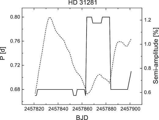
The evolution of period (solid line) and amplitude (dashed line) of the light curve of HD 31281 during the C4 campaign of the K2mission. See text for details.
The analysis of ground-based observations by SuperWASP and NSVS and Kepler data yielded the same result for star HD 286179, namely P ∼ 3.1397(21) days and P ∼ 3.1249(20) days, respectively. This value is smaller than previously reported by Bouvier et al. (1997) (3.33 days). A harmonic 1:2 period peak was also found in the C13 data set. We have folded the Kepler light curve using both test periods (Fig. S7). After inspecting the resulting phase curve visually, we have adopted the period P = 3.1249 days. The origin of period P = 0.9272(621) days in season 3 of SuperWASP is likely the result of fewer data in comparison with other seasons.
When analysing data of HD 286178, we found the most prominent period to be P ∼ 1.7 days. This is the 1:2 harmonic of P = 2.39 days reported by Bouvier et al. (1997). However, in our season 4 (2008–2009), we have found the most prominent period to be ∼2.37 days. Data of Bouvier et al. (1997) were obtained during years 1994–1996. The change in observed period can be explained e.g. by the emergence of a previously unobserved area of photospheric spots. This would result in a shorter photometric period of ∼1.7 days. We have repeated the period analysis with all the ground-based data binned to a single point per night spanning 12.5 years. The subsequent period analysis showed only one peak at P ∼ 2.4 days. We are thus inclined to consider the rotation period to be close to this value. The Kepler data set revealed prominent peaks at P = 1.7027(6), 2.3562(11) and 1.1813(3) days (ordered with decreasing power). Also, the wavelet analysis showed a sudden change in period from ∼2.36 to ∼1.70 days (see Fig. 5). Based on the distance of 74.3 pc of HD 286178 (from Table 1), stellar properties R = 1.04 R⊙, L = 0.71 L⊙ and a reliable estimate of AV, we can write
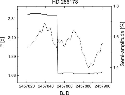
The evolution of period (solid line) and amplitude (dashed line) of the light curve of HD 286178 during the C13 campaign of the K2mission. See text for details.
If we use the value v sin i = 42 km s−1 from Wichmann et al. (2000), we obtain values for sin i. However, only for period P = 1.1813(3) days is sin i ≤ 1, which disallows the other periods P = 1.7027(6) days and 2.3562(11) days from further analysis.
HD 283447 had a previously reported period P ∼ 51 days (Welty 1995). The star was described as an SB2 system with K-type components. From the photometric point of view, we have not found any signal corresponding to this period, i.e. the measured variations in flux are due to changes in the visible photosphere. We have found a period P = 3.0836(210) days with an amplitude ∼2 × the diurnal period.
HD 285778 was found to have a mean period of ∼2.7361(204) days from the ground-based data, which confirms the period previously determined by Grankin (2013). This object was also the only one from our sample to have two Kepler data sets available. In the C4 season, an additional period was found. We have folded the data using both test periods (the result is shown in Fig. S7). The descending slope between phases 0.2 and 0.8 folded with the period P = 2.8554 days is closer to the descending slope of the original light curve. The dubious period from the NSVS data, 0.9951(333) days, is most probably a window alias. The determination of a 0.9801(879) day period from season 3 was plagued by the low number of data points. In season 2, the period found was close to 1:2 and is caused by spots distributed by ∼180º on the surface of the star.
The most intriguing object is HD 283518 (V410 Tau). This is a well-investigated star (see e.g. Stelzer et al. 2003; Grankin & Artemenko 2009). The phase light curve of the whole data set (Σ) shows a clear frequency wave (see Fig. 6) when folded with the most prominent period. The period analysis based on the whole data set yielded two distinct peaks (Fig. 7) at P = 1.8758 days and P = 0.9338 days (ordered by their respective amplitude). We have to apply the DC DFT analysis for separate seasons (0–2 and 5–7, see Table 3 for the dates of observations). Except for season 6, we have found the mean period ∼1.87 day. To fit the light curve properly, we had to add the next harmonic frequency, corresponding roughly to P2 ∼ 0.936 days. Phased light curves with a fit are presented in Fig. 8. The added harmonic period can be interpreted as due to the presence of at least another spot located almost opposite the first spot area. Detailed spot configuration would need to be carried out using Zeeman–Doppler imaging and a surface inversion technique.
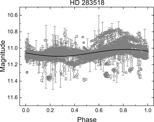
Light curve of all available photometry from SuperWASP and NSVS data for HD 283518 folded with the mean period P = 1.8706 days.
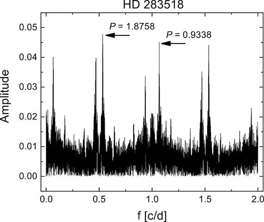
Fourier plot of the whole data set (Σ) for HD 283518. Most prominent periods are marked. Other peaks are aliases from the spectral window.
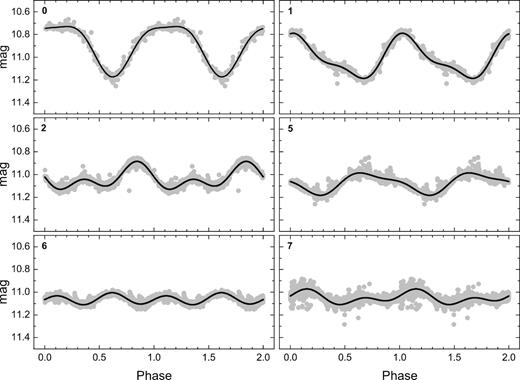
Evolution of the phased light curve of star HD 283518 in different observational seasons (panel number). The most dominant frequency in each season (see Table 4) was used to construct the phased light curve. The solid line represents a fit with the addition of the first harmonic frequency.
5 CONCLUSIONS
We have performed a thorough period analysis of 20 selected weak-line T Tauri stars based on data available from the NSVS and the SuperWASP archive. For two objects (HD 283782 and HD 31281), we made the first estimate of the photometric period. We have also found a more reliable period estimate for HD 283798. Period analysis based on all available data leads to the confirmation and update of periods previously published in the literature in 15 cases (up to 10 per cent difference).
The main advantage of these period estimates is that we have analysed a very long time interval (up to ∼12.5 years). Fortunately, our targets with dubious periods were also observed by the K2mission, which allowed us to distinguish the mean photometric periods from their harmonic components. We have also performed wavelet analysis for our stars observed by Kepler and searched for their period evolution. The sudden change of period in several targets can be explained by the emergence of another photospheric spot, which remained visible for several days.
We have constructed a simple spot model, with the possibility of adding and removing spots to compute long artificial light curves. After that, a period search and wavelet analysis were applied. We found that (i) Fourier analysis found only a median period, but WWZ converged on the intrinsic rotational period, (ii) additional spots increased the amplitude and the most significant Fourier period of the light curve, (iii) period evolution was gradual if spots were close to each other and (iv) spots placed almost on the opposite sides of the stellar disc generated a rapid change between Prot and Prot/2.
Using WWZ to investigate the period evolution can place further limits on the possible rotation period. A full model could deal with unknown inclination of the stellar rotational axis, differential rotation and spot migration. A light curve with very good sampling and long temporal duration is needed for such a model.
The light curves of HD 283518 (V410 Tau) were analysed sepearately for six individual observing seasons. The comparison of our study with past data hinted that the evolution of light-curve variations caused by changes in the distribution of cool photospheric spots may be the result of a ∼15-year long cycle similar to the 11-year cycle of the Sun.
The evolutionary status of our targets was checked using accurate parallaxes and mean stellar parameters from the literature and calibrations of the Strömgren–Crawford uvbyβ photometric system. Thanks to the already published Gaia DR2 data, the luminosities are already very accurate, with the largest uncertainty contribution coming from the a priori unknown reddening. Furthermore, the uncertainties in the effective temperatures prevent a suitable calibration of age and mass to correlate these parameters with the rotational periods.
Therefore, we are continuing our investigation on selected targets with dedicated spectroscopic observations to provide accurate and homogeneous effective temperatures.
SUPPORTING INFORNATION
Additional Supporting Information may be found in the online version of this article:
Figures S1 and S2. Fourier plots of investigated targets from ground-based observations.
Figure S3. Fourier plots of targets with available Kepler photometry.
Figures S4 and S5. Light curves of investigated targets phase-folded with periods estimated from a single season.
Figure S6. Light curves of targets observed by Kepler.
Figure S7. Phased light curves of targets with more than one prominent period in the Kepler data.
Figure S8. Evolution of period and amplitude of light curves of our Kepler targets.
Please note: Oxford University Press is not responsible for the content or functionality of any supporting materials supplied by the authors. Any queries (other than missing material) should be directed to the corresponding author for the article.
ACKNOWLEDGEMENTS
This study has been supported by the projects VEGA 2/0143/14, VEGA 2/0031/18, APVV-15-0458 and 7AMB17AT030 (MŠMT). This article was created by the realization of the project ITMS No.26220120029, based on the supporting operational research and development program financed from the European Regional Development Fund. This work has made use of data from the European Space Agency (ESA) mission Gaia (https://www.cosmos.esa.int/gaia), processed by the Gaia Data Processing and Analysis Consortium (DPAC, https://www.cosmos.esa.int/web/gaia/dpac/consortium). Funding for the DPAC has been provided by national institutions, in particular the institutions participating in the Gaia Multilateral Agreement. This article includes data collected by the Kepler mission. Funding for the Kepler mission is provided by the NASA Science Mission directorate. Some/all of the data presented in this article were obtained from the Mikulski Archive for Space Telescopes (MAST). STScI is operated by the Association of Universities for Research in Astronomy, Inc., under NASA contract NAS5-26555. Support for MAST for non-HST data is provided by the NASA Office of Space Science via grant NNX09AF08G and by other grants and contracts. This research was made possible through the use of the AAVSO Photometric All-Sky Survey (APASS), funded by the Robert Martin Ayers Sciences Fund. We thank the reviewer for the thorough review and highly appreciate the comments and suggestions, which contributed significantly to improving the quality of the publication. This work was based on data from SuperWASP and NSVS archives.
