


ABSTRACT
We present 1.3 and 3.2 mm continuum maps of three star-forming regions in the Large Magellanic Cloud (LMC) observed with the Atacama Large Millimeter/Submillimeter Array (ALMA). The data were taken from two projects retrieved from the ALMA public archive and from one project observed specifically for this work. We develop a technique to combine maps at these wavelengths to estimate dust-only emission corrected for free–free emission contamination. From these observations, we identify 32 molecular clumps in the LMC and estimate their total mass from their dust emission to range from 205 to 5740 |$\mathrm{M}_{\odot}$|. We derive a cumulative clump mass function (N(≥M) ∝ Mα + 1) and fit it with a double power law to find |$\alpha _{\mathrm{low}} = -1.76^{+0.04}_{-0.05}$|, αhigh = −3.3 ± 0.2, with a break mass of |$2500^{+300}_{-200}$||$\mathrm{M}_{\odot}$|. A comparison with the 30 Doradus-10 mass function derived previously from CO (2–1) data reveals a consistent range of clump masses and good agreement between the fitted slopes. We also find that the low-mass index of the LMC mass function agrees well with the high-mass index for core and clump mass functions from several star-forming regions in the Milky Way. This agreement may indicate an extension of the Milky Way power law to higher masses than previously observed.
1 INTRODUCTION
Millimetre observations beyond the Milky Way are beginning to probe the scales of clustered and individual star-forming regions known as molecular gas clumps and cores. While filamentary structure has previously been shown to be ubiquitous in Galactic star-forming molecular gas (André et al. 2010; Arzoumanian et al. 2011; Könyves et al. 2015) and in other galaxies (the Large Magellanic Cloud in carbon monoxide (CO): Fukui et al. 2008; Wong et al. 2011), it is the higher-density clumps and cores within the filaments that directly set the initial conditions for the formation of stars and clusters.
The choice of these functional forms is motivated by the tendency for the mass functions to have a long tail at high masses and a flatter portion or turnover at low masses. Physically, the power-law tail has been attributed to collapse in molecular clouds in whichgravity is dominating the motions (Ballesteros-Paredes et al. 2011), although analysis of simulated and analytic cloud column-densities has shown the power-law tail occurs as a result of the appearance of strong density peaks in molecular clouds, not the transition to gravity-dominated dynamics (Tassis et al. 2010). Lognormal forms have been argued for as following from the density distribution of supersonic turbulence (Padoan, Nordlund & Jones 1997), although the presence of supersonic turbulence is not necessary for the density distribution to exhibit a lognormal shape (Tassis et al. 2010). The combination of various independent stochastic processes impacting the distribution of molecular gas in clouds has been shown to lead to a lognormal distribution through the central limit theorem (Larson 1973; Adams & Fatuzzo 1996). However, observational evidence for the ubiquity of lognormal distributions may be more difficult to confirm than previously thought (Alves, Lombardi & Lada 2017).
In addition to comparing mass distributions between different regions, core mass functions have also been compared to the similarly shaped stellar IMF. Chabrier (2003, 2005) showed that the stellar IMF follows the original Salpeter (1955) power-law index of −2.35 ± 0.3 above 1 |$\mathrm{M}_{\odot}$|, with a lognormal turnover at low masses peaking at about 0.2 |$\mathrm{M}_{\odot}$|. This mass distribution has been observed to be universal across environments such as the Galactic disc, young and globular star clusters, and the spheroid or stellar halo (Chabrier 2003, 2005; Krumholz 2014). A similar power-law slope has been predicted for the stellar IMF and core mass functions (Chabrier & Hennebelle 2010; Guszejnov & Hopkins 2015). The observed similarity in slopes has led to the idea that there exists a star formation efficiency that is independent of mass and is acting to transform the core mass function to the IMF (Alves, Lombardi & Lada 2007; André et al. 2010; Könyves et al. 2015).
At higher masses, the comparison is between the mass distributions of entire star clusters and the clump mass functions within their natal GMCs (Lada 1992). Lada & Lada (2003) compiled a list of 76 young star clusters still embedded within a GMC and from this derived a cluster mass function with a power-law index of −2 between ∼50 and 1000 |$\mathrm{M}_{\odot}$|. Fall & Chandar (2012) found that the mass functions of star clusters from six galaxies were all well fitted by power laws with indices close to −1.9.
Given the wealth of information gathered on the mass distributions of cores and clumps in the Milky Way, the next step is to extend these studies to other galaxies. This provides new physical environments in which to test models, as well as larger samples from which to draw statistical conclusions. Two of our nearest neighbours, the Magellanic Clouds, are now well within the reach of mm/submm observations of molecular and dust emission for studies of the clump mass function. For example, Indebetouw et al. (2013) derived a CO mass function of 103 clumps at 0.46-pc resolution in the Large Magellanic Cloud (LMC) with the Atacama Large Millimeter/Submillimeter Array (ALMA). While extension beyond the Magellanic Clouds promises a further variety of environments and larger sample sizes, such studies push even the most advanced observatories to their limits. Rubio et al. (2015) reported on 10 CO clouds in the Wolf–Lundmark–Melotte (WLM) galaxy with masses of 5900 to 7.3 × 10⁴ |$\mathrm{M}_{\odot}$|. At a distance of 1 Mpc, they achieved ∼5-pc resolution with ALMA. More recently, Schruba et al. (2017) observed NGC 6822 with ALMA, reaching 2-pc resolution at a distance of 470 kpc. A total of 156 CO clumps were extracted with masses of 9 to 3500 |$\mathrm{M}_{\odot}$|. Thus, if we wish to sample the full range of clump sizes and even to start to probe molecular core scales, we are limited to the nearest Local Group members.
The LMC is the ideal next step after our Galaxy for the study of resolved star formation, given its proximity (49.97 ± 1.11 kpc, Pietrzyński et al. 2013) and nearly face-on orientation. It is also a system that is significantly different from the Milky Way in which to study how stars form, with a lower average metallicity of ∼(1/3)–(1/4) |$\mathrm{Z}_{\odot}$| (Rolleston, Trundle & Dufton 2002; Dufour 1984). The lower metal abundance results in smaller quantities of dust and thus in less shielding for star-forming regions from ultraviolet (UV) radiation. This means that molecular gas reservoirs may be lower in mass (Fukui et al. 1999, 2001), which limits the star-forming fuel throughout the galaxy. The presence of fewer metals also means that cooling through line emission is reduced, which can change the energy balance in molecular clouds. Finally, the characteristic peak mass of the stellar IMF has been predicted to shift to higher masses for low metallicity (Bromm 2005, albeit for near-zero metallicity conditions).
In this paper, we calculate and analyse the dust-derived clump mass function in the LMC in order to facilitate comparison with mass functions of star-forming regions in the Milky Way. In Section 2 we summarize the observations from each ALMA project we used and we describe our continuum map-making process. In Section 3 we describe our method of isolating the dust-only emission in each region, our clump identification procedure, and the steps we took to fit and characterize our final mass function. In Section 4 we discuss our results from Section 3 and place them in the broader context of the study of molecular clump mass functions. The paper is summarized in Section 5. Maps of each field included in our mass function are presented in Appendix A as observed emission as well as being decomposed into dust-only and free–free-only emission.
2 OBSERVATIONS AND DATA REDUCTION
2.1 Spatial and spectral setups
We retrieved six publicly available projects from the ALMA archive containing observations of seven fields in the LMC covering the star-forming regions 30 Doradus-10 (30 Dor-10), N159W, N159E, N113, N166, GMC 225 and PCC 11546. In addition, we obtained new data in Cycle 4 towards 30 Dor-10 with the 7-m Atacama Compact Array (ACA). The projects were observed between 2011 December 31 and 2017 April 21, spanning Cycles 0, 1, 2 and 4.
For all but one region, multiple pointings were observed across each field in both bands to produce mosaic maps. Mosaic pointings were roughly Nyquist-spaced in a given band in order to achieve relatively uniform coverage across the inner portion of the maps when imaged together. 12-m (main array) plus ACA data were obtained for all fields except N113, which was observed as a single pointing and only with the main array. The number of pointings on a field and in a single band ranged from 1 (N113) to 170 (N166). Mapped areas cover between 0.21 arcmin2 (N113) and 7.5 arcmin2 (N166; refer to Table 3 for the areas of each field in both bands).
In order to measure dust masses in molecular clumps we focused on continuum observations from 86 to 100 GHz (∼3.2 mm) and from 217 to 233 GHz (∼1.3 mm) in ALMA bands 3 and 6, respectively. Observations at these frequencies are likely to contain significant emission from sources other than thermal dust, such as free–free emission. The effective bandwidths used in making the continuum maps ranged between 1.6 and 4 GHz. The locations of the regions analysed here are marked on the infrared image of the LMC in Fig. 1, and a summary of the observational details is given in Table 1.
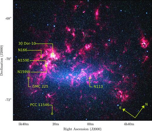
SAGE Spitzer IRAC three-colour image of the Large Magellanic Cloud (Meixner et al. 2006). Red, green and blue are 8, 4.5 and 3.6 |$\mu$|m maps, respectively. The positions of the seven regions discussed in this paper are labelled.
ALMA projects used in this paper.
| RAa | Dec.a | |||
|---|---|---|---|---|
| [J2000] | [J2000] | |||
| Field name | [h:m:s] | [°:′:″] | Project code | Ref.b |
| 30 Dor-10 | 05:38:48 | −69:04:48 | 2011.0.00471.S | 1 |
| 30 Dor-10 | 05:38:48 | −69:04:48 | 2016.1.01533.S | 2 |
| N159W | 05:39:37 | −69:45:48 | 2012.1.00554.S | 3 |
| N159E | 05:40:09 | −69:44:44 | 2012.1.00554.S | 4 |
| N113 | 05:13:18 | −69:22:25 | 2013.1.01136.S | 5 |
| GMC 225 | 05:47:09 | −70:40:16 | 2012.1.00603.S | 6 |
| GMC 225 | 05:47:09 | −70:40:16 | 2013.1.01091.S | 6 |
| N166 | 05:44:29 | −69:25:43 | 2012.1.00603.S | 6 |
| N166 | 05:44:29 | −69:25:43 | 2013.1.01091.S | 6 |
| PCC 11546 | 05:24:09 | −71:53:37 | 2013.1.00832.S | 7 |
Notes. aPhase centre is given for multipointing mosaics or the pointing centre for single-pointing observations (N113).
2.2 Background on individual fields
The Tarantula Nebula, or 30 Doradus, is one of the most active star-forming regions in the LMC. It harbours the R136 star cluster, which boasts stellar densities of between 104 and 107 |$\mathrm{M}_{\odot}$| pc−3 (Selman & Melnick 2013). Multiple generations of star formation have occurred in 30 Doradus over the course of ∼20 Myr (De Marchi et al. 2011; Walborn & Blades 1987). 30 Doradus has been observed as part of several LMC-wide surveys targeting various emission sources. In CO, it has been observed with theNANTEN telescope in 12CO (1–0) (Fukui et al. 2008) and with the Mopra telescope in 12CO and 13CO (1–0) (Hughes et al. 2010; Wong et al. 2011). The HERITAGE Key Project Survey (Meixner et al. 2013) observed it in dust emission along with the rest of the LMC.
The GMC 30 Dor-10 (Johansson et al. 1998) is part of the Tarantula Nebula, and is within a projected distance of 11 pc from R136. Indebetouw et al. (2013) observed 30 Dor-10 with ALMA in 12CO and 13CO (2–1) emission as well as the 1.3-mm dust continuum at ∼1.9-arcsec resolution. The dust map was used to derive a total H2 mass for the GMC of (6 ± 1) × 104 |$\mathrm{M}_{\odot}$|. Clump apertures identified in their 12CO and 13CO cubes were used to calculate independent H2 masses from both the dust and the CO data. Indebetouw et al. (2013) calculated a CO-derived mass function for their 103 clumps and fitted it with a power law of α = −1.9 ± 0.2.
N159 was originally identified by Henize (1956) as an H ii region and has since been extensively studied. Noted as the strongest CO-intensity cloud in the initial NANTEN LMC survey (Fukui et al. 2008), N159 has been resolved into three major clumps, namely N159W, N159E and N159S (Johansson et al. 1994). Across the region, multiline excitation analyses on ∼10-pc scales estimated molecular gas kinetic temperatures ranging from 10 to 25 K (Heikkilä, Johansson & Olofsson 1999; Bolatto et al. 2000). ALMA observations of N159W suggest that its constituent group of compact H ii regions may have formed through a cloud–cloud collision (Fukui et al. 2015). By adding a dynamical estimate of one of the young stellar objects (YSOs) of 104 yr, Fukui et al. (2015) showed that the collisional triggering of star formation probably occurred very recently. N159E contains multiple developed H ii regions, the most prominent of which is the Papillon Nebula (Mizuno et al. 2010). Saigo et al. (2017) suggested that a three-cloud collision is occurring in N159E, with the Papillon Nebula protostar in the overlap region. They also observed a molecular hole around the protostar filled with 98-GHz free–free emission, indicating that the protostar has recently begun disrupting the molecular cloud from which it formed. N159S does not exhibit any current star formation.
N113 was also identified by Henize (1956) as an H ii region. Observed as part of a sample of four molecular clouds (N159W, N113, N44BC and N214DE) with the Swedish-ESO Submillimetre Telescope (SEST), it exhibited significantly lower gas-phase C18O/C17O abundances compared with molecular clouds in the Milky Way and the centres of starbursts, with a mean across clouds of 1.6 ± 0.3 (Heikkila, Johansson & Olofsson 1998). Subsequent observations have shown it to contain the most intense maser in the Magellanic Clouds (Imai et al. 2013), clumpy molecular gas currently forming stars (Seale et al. 2012), and a host of YSOs as identified by Herschel and Spitzer (Ward et al. 2016). N113 is related to three young stellar clusters (NGC 1874, NGC 1876 and NGC 1877; Bica, Claria & Dottori 1992). It also contains a rich assortment of molecular species (Paron et al. 2014).
N166 is yet another region originally identified by Henize (1956), and Fukui et al. (2008) determined that it contained only H ii regions. Two molecular clouds were observed overlapping its position in the second NANTEN survey, and a follow-up observation with ALMA targeted a position between these two NANTEN-observed clouds. N166 was also observed with the Atacama Submillimetre Telescope Experiment (ASTE) in 12CO (3–2), revealing densities of 102 to 103 cm−3 and kinetic temperatures between 25 and 150 K in a 22-arcsec beam (Paron et al. 2016).
GMC 225 is one of 272 GMCs identified by Fukui et al. (2008) in the second NANTEN survey of the LMC in 12CO (1–0) and shows no sign of massive star formation (Kawamura et al. 2009). With a CO-derived total mass of 106 |$\mathrm{M}_{\odot}$| and a radius of ∼73 pc, it was observed as part of a follow-up ALMA project. It is ∼1500 pc south of 30 Dor-10 and east of the molecular ridge.
PCC 11546 is an extremely cold (≲15 K) dust source identified in the southern limits of the LMC as part of the Planck Galactic Cold Cloud catalogue (Planck Collaboration et al. 2016). It also exhibits strong CO (1–0) emission in the Planck integrated CO map and the MAGMA LMC CO survey (Wong et al. 2011). There appears to be a lack of massive star formation within PCC 11546, and it contains lower-density gas than clouds closer to the centre of the LMC (Wong et al. 2017).
2.3 Calibration
The visibility data were retrieved from the archive and calibrated. All fields except 30 Dor-10 had only raw data available in the archive. 30 Dor-10 had calibrated visibilities available, and we used those data after recalculating the weights based on the scatter in the visibilities using the Common Astronomy Software Applications (casa) ‘statwt’ command.
The observations with raw data available were either ‘manually’ or pipeline-calibrated at the observatory using casa (McMullin et al. 2007). For manually calibrated data, we ran the full calibration procedure using the observatory scripts in the latest version of casa available at the time, 4.7.2-REL (r39762). Minor editing of the calibration scripts was necessary in order to account for task and parameter changes from the older versions of casa. Edits were also made to ensure that the visibility weights were properly calculated throughout the entire calibration procedure.
For pipeline-calibrated data, we used the casa and pipeline versions closest to those used by the observatory for the original calibration.1 There was no concern regarding visibility weights because all publicly available pipeline releases were after casa 4.2.2, which contained a major correction to the handling of the weights.
Once the calibrated data were obtained we inspected the visibilities from the calibrator sources to ensure that the results of the calibration were as expected and that all seriously problematic data were flagged. In most cases this inspection did not reveal anything that needed to be done beyond the observatory-provided calibration process. A few cases, however, did expose situations where marginal antennas or edge channels should have been flagged, and we did so before imaging.
2.4 Imaging
All imaging steps, from inspecting the visibilities up to and including cleaning the maps, were carried out in casa 4.7.22 (r39762) for all fields. Strong emission lines were identified with the plotms task and flagged before the visibilities were imaged to produce continuum maps. Because we combined maps in the two bands to create a dust-only emission map, we needed to match the spatial scales to which each pair of maps is sensitive as closely as possible. Matching the spatial-scale sensitivities was achieved through a combination of trimming the shortest uv-spacings and tapering the weighting of the longest uv-spacings. In order to choose which inner uv-trimming to use (the minimum uv-distance to include in imaging), we plotted the source visibility amplitudes versus their radial uv-distance in wavelengths for each band. The longer minimum baseline length of the two was used as the minimum uv-distance to include. For our fields, this minimum uv-distance was always set by the Band 6 data, so the uv-distance trimming was always applied to the Band 3 data.
The outer uv-tapering directly changes the synthesized beam and sets the smallest spatial scale in the cleaned maps. The Band 6 maps always had smaller initial synthesized beams than the Band 3 maps. Once the uv-distance trimming was applied to the Band 3 data, we used the Band 3 synthesized beam as the target beam shape for the Band 6 uv-tapering.
Matching the beam shapes precisely through tapering alone was not possible given the differences in intrinsic uv-coverage between the observations. Therefore, we used the ‘restoringbeam’ parameter in clean to force the Band 6 Gaussian beam shape to be the same as that of the Band 3 map. Note that this means that all noise and any emission left in the residual maps is still at the tapered resolution, and only the emission that was cleaned is exactly matched to the Band 3 resolution. However, we were always able to bring the beams into fairly close agreement with the uv-tapering. The differences between the Band 6 and Band 3 beam axes were <10 per cent (and usually much less), and position angle differences were <5 per cent. Only 30 Dor-10 had a larger position angle difference (∼30° versus ∼60°).
We cleaned all the dirty maps that showed obvious emission, which meant that N166, GMC 225 and PCC 11546 were not cleaned. Motivated by the complexity of the emission in the 30 Dor-10 maps and by the desire to have a reproducible method of producing cleaned maps, we implemented an auto-masking algorithm for all cleaning. This algorithm is heavily based on the auto-masking code given in the M100 casa Guide as it appeared in 2016 August. We modified it to work as an automated casa script:3 when given a set of clean parameters, a minimum threshold to clean down to, a casa region text file specifying an emission-free region of the dirty map, and a minimum spatial size to mask, the script iteratively cleaned down to the desired threshold. All auto-masking was carried out with stopping thresholds between 1.5 and 3 times the noise in the map and using minimum mask areas of 0.5 times the map synthesized beam. All fields were cleaned with Briggs weighting (Briggs 1995),4 with the ‘robust’ parameter set to 0.5, and in multifrequency synthesis mode, with ‘psfmode’ set to ‘psfclark’ and using a maximum of 104 iterations. Table 2 lists the values used for important clean parameters for each field. The average synthesized beam size was ∼2.3 arcsec, corresponding to ∼0.6 pc at the distance of the LMC. Mapped areas cover between 44 (N113) and 1600 pc2.
Important clean parameters used in imaging.
| ‘outertaper’c | |||||||||
|---|---|---|---|---|---|---|---|---|---|
| ‘cell’a | ‘imsize’a | ‘threshold’a | ‘uvrange’ | ‘minpb’ | ‘robust’ | Major axis | Minor axis | Position angle | |
| Field name | [arcsec] | [pixels] | [mJy bm-1] | (>λ) | [arcsec] | [arcsec] | [°] | ||
| 30 Dor-10 | 0.18 | 1152, 750 | 0.30, 0.78 | 5092 | 0.38 | 0.5 | 0.85 | 0.1 | 67 |
| N159W | 0.213 | 1000, 720 | 0.96, 1.32 | 8023 | 0.4 | 0.5 | 2.76 | 1.64 | 81 |
| N159E | 0.21 | 1250, 750 | 0.80, 1.78 | 5956 | 0.5 | 0.5 | 3.05 | 1.45 | −70 |
| N113 | 0.13 | 1250, 750 | 0.40 | ... | 0.5 | 0.5 | ... | ... | ... |
| GMC 225 | 0.32, 0.11 | 700, 1500 | ... | ... | 0.5 | 2 | ... | ... | ... |
| N166 | 0.38, 0.155 | 1050, 1568 | ... | ... | 0.5 | 2 | ... | ... | ... |
| PCC 11546 | 0.126 | 1680 × 2400b | ... | ... | 0.5 | 2 | ... | ... | ... |
Notes. Column headings are clean task parameter names.
aFor fields with two entries, the Band 3 value is reported first and the Band 6 value second.
bSquare maps were made for all fields except PCC 11546.
cApplied to the Band 6 data only.
2.5 Fields without detections
We tried to improve the signal-to-noise ratio (S/N) in the maps with no continuum emission by setting ‘robust’ to 2.0 to favour S/N over resolution. While the noise did drop, it was not enough to enable emission to be detected in any of the non-detection maps. The rms noise and beam shapes listed in Table 3 for GMC 225, N166 and PCC 11546 refer to the maps made with ‘robust’ set to 2.0.
Image properties for each Large Magellanic Cloud field.
| Map areaa | Synthesized beamb | Noised | |||||||
|---|---|---|---|---|---|---|---|---|---|
| Band 3 | Band 6 | Bandwidthb, c | Major | Minor | P. A. | Dust | Band 3 | Band 6 | |
| Field name | [arcmin2] | [arcmin2] | [ GHz] | [arcsec] | [arcsec] | [°] | [mJy bm-1] | ||
| 30 Dor-10 | 1.9 | 1.2 | 4 | 2.25 | 1.40 | 65 | 0.41 | 0.15 | 0.39 |
| N159W | 1.9 | 1.6 | 1.9, 1.6 | 2.63 | 1.67 | 82 | 0.50 | 0.64 | 0.53 |
| N159E | 1.8 | 1.8 | 1.9, 1.6 | 2.90 | 1.61 | −77 | 0.66 | 0.32 | 0.60 |
| N113 | ... | 0.21 | 2.5 | 1.35 | 1.04 | 61 | ... | ... | 0.26 |
| GMC 225 | 4.0 | 3.4 | 1.9 | 4.26, 2.01 | 3.13, 1.13 | −67, −86 | ... | 0.18 | 0.76 |
| N166 | 7.5 | 4.0 | 1.9 | 4.08, 2.17 | 3.57, 1.61 | −73, 69 | ... | 0.20 | 0.94 |
| PCC 11546 | ... | 5.8 | 3.4 | 1.81 | 1.23 | 75 | ... | ... | 0.19 |
Notes. Synthesized beam-shape parameters are given for the final images used to create our clump mass function.
aArea of the mapped field above a gain response threshold of 0.5. Dust-only maps are only defined where both Band 3 and Band 6 data overlap, so dust-only map areas are the same as the Band 6 maps. At the distance of the Large Magellanic Cloud, 1 arcmin2 ≈ 212 pc2.
bFor fields with two entries, the Band 3 value is reported first and the Band 6 value second.
cApproximate bandwidth of continuum data used to produce the final maps. Bright emission lines are excluded in this estimate and in continuum imaging.
dNoise measurements were made in emission-free regions of the dirty map for each field.
Almost half of the fields we investigated were not detected in continuum emission. This raises the question whether the data for these fields are inherently of poorer sensitivity than the data with abundant emission. We tested this by matching the synthesized beams across all fields to the largest beam in each band. At 3.2 mm, GMC 225 and N166 have the lowest rms noise in our sample by a factor of 2–6. The 1.3-mm observations of PCC 11546 have a smaller rms noise than the fields with detections, and the sensitivities of GMC 225 and N166 at this wavelength are only a factor of 2–3 worse. This comparison suggests that there are intrinsic differences in the physical densities and structures of the non-detection fields compared with those of the four detected regions.
3 DATA ANALYSIS
3.1 Free–free correction
Given the frequencies of these observations, we expect the main contributions to continuum emission to be thermal emission from the ∼30 K dust and free–free emission from ionized gas. Although synchrotron emission is another possible source of continuum emission at these frequencies, H ii regions, protostars and young stars do not produce much synchrotron emission (Ginsburg et al. 2016). Colliding-wind binaries have been observed with spectral indices indicative of synchrotron radiation from particles accelerating in the wind collision zone (De Becker & Raucq 2013). However, following the method of Ginsburg et al. (2016), we estimate a 3.2-mm flux density of ∼6 µJy per binary. These flux densities are 30 to 100 times smaller than the noise in our fields (Table 3).
Fig. 2 compares the 1.3- and 3.2-mm fluxes for clumps identified in the 1.3-mm map. The solid line shows the flux scaling for free–free emission with exponent −0.1, and the two dashed lines show dust emission with exponents (2 + β) for β = 1 and β = 2. Because the points are clustered between the free–free and dust scaling relationships, we conclude that there is significant free–free emission even at 1.3 mm. In order to use the dust emission to estimate the total mass of the clumps in these fields we need to correct for contamination from free–free emission at 1.3 mm.
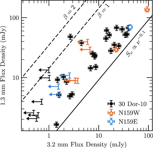
Comparison of 3.2-mm (Band 3) and 1.3-mm (Band 6) flux densities for clumps identified at 1.3 mm. The dashed lines show two different thermal dust emission scaling relationships covering the range of realistic dust emissivity spectral indices, and the solid line shows a typical free–free scaling relationship. Upper limits at 3.2 mm are for clumps found at 1.3 mm without significant co-spatial emission at 3.2 mm. Error bars correspond to a 10 per cent calibration uncertainty.
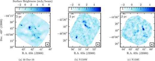
Dust-only maps of (a) 30 Dor-10, (b) N159W and (c) N159E made from the combination of 3.2- and 1.3-mm ALMA observations. Contamination from free-free emission has been removed from these maps using equation (6).
We tested our algebraic decomposition using lower-frequency radio observations that are often used to measure free–free and synchrotron emission directly. Observations at 4.8 GHz (6 cm) and 8.4 GHz (3 cm) were made of 30 Doradus (Lazendic, Dickel & Jones 2003) and N159 (Indebetouw, Johnson & Conti 2004) with the Australia Telescope Compact Array (ATCA). We applied spatial filtering to the radio images, to match the ACA uv-coverage of the ALMA observations, through the casa observation simulation functionality. This allowed us to better match the spatial scales measured at the two frequencies (especially for 30 Dor-10, where the ACA uv-coverage filtered out about 50 per cent of the radio flux).
We first measured the total fluxes in each field at 4.8 and 8.4 GHz. Adopting a synchrotron spectral index of −0.83 and a free–free spectral index of −0.1, we iterated in order to estimate the balance of the two emission sources at the two frequencies. We then extrapolated the free–free component to the ALMA Band 3 frequency to obtain an estimate of the expected free–free emission at 3.2 mm.
To compare this estimate with observations, we solved for the free–free-only emission in Band 3 (see Appendix A for specific decomposition expressions and maps of free–free-only emission). Assuming a 10 per cent absolute flux calibration uncertainty on the radio continuum, the total free–free emission in 30 Dor-10 matches within 15 per cent between extrapolated and decomposed estimates (0.82 and 0.97 Jy, respectively). N159W is consistent within the radio uncertainties, with flux densities of 75 and 78.5 mJy in the ATCA and ALMA maps, respectively.
N159E appears to have about four times too much free–free flux in Band 3 when compared with the extrapolated flux (it has a near-synchrotron-only spectral index in the radio maps). If the free–free emission becomes optically thick between 8.6 and 98 GHz then the free–free spectrum would turn over (e.g. Turner, Ho & Beck 1998), leaving just the synchrotron spectral index and a low free–free flux at low frequencies. Galactic ultracompact H ii regions have been observed with free–free spectral turnovers at frequencies between 10 and 20 GHz (Wood & Churchwell 1989). It is possible that the main region of bright radio emission is originating from a population of ultracompact H ii regions averaged together with supernova remnants within the ALMA beam, leading to synchrotron-dominated emission near 10 GHz and the presence of free–free emission at and above 100 GHz.
Finally, we estimate that diffuse synchrotron emission contributes up to ∼12 per cent of the Band 3 flux. Because our method scales between Band 3 and Band 6 with the free–free spectral index, this synchrotron component is oversubtracted from the Band 6 flux by equation (6). This results in, at most, 4 per cent of the total Band 6 flux being oversubtracted when making the dust-only maps as a result of neglecting a synchrotron term in equation (6). Considering the imperfect uv-coverage matching between the ATCA and ALMA observations and the 10 per cent calibration uncertainty on the ALMA and ATCA observations, we believe that the radio free–free emission estimates agree well enough and that the synchrotron is weak enough in Band 6 that we can continue with our algebraic method.
We are not able to include N113 in our final mass function analysis because of the non-trivial free–free emission illustrated in Fig. 2 and our lack of observations at 3.2 mm for this field. Not being able to include N113 was unfortunate because this object contributed about the same number of clumps in Band 6 as the N159E map, even within the much smaller area.
3.2 Clump finding
In order to identify molecular gas clumps in our dust-only maps we used the ClumpFind algorithm (Williams, de Geus & Blitz 1994) available in starlink5 through the cupid package (Berry et al. 2007). We chose to use this algorithm to facilitate direct comparison with previous work that also used ClumpFind. A total of 32 dust clumps were identified in three fields (30 Dor-10, N159W and N159E), with the majority found in 30 Dor-10. Clump properties are summarized in Table 4.
Properties of clumps in the Large Magellanic Cloud.
| RAa | Dec.a | Areab | |$S_{\mathrm{ff,peak}}\, ^{c,d}$| | |$S_{\mathrm{ff,int}}\, ^{c,e}$| | |$S_{\mathrm{d,peak}}\, ^{f,g}$| | |$S_{\mathrm{d,int}}\, ^{f,h}$| | Mi | |
|---|---|---|---|---|---|---|---|---|
| [J2000] | [J2000] | |||||||
| Name | [h:m:s] | [°:′:″] | [pc2] | [mJy bm−1] | [mJy] | [mJy bm−1] | [mJy] | [|$\mathrm{M}_{\odot}$|] |
| 30 Dor-10 1 | 05:38:49.22 | −69:04:42.24 | 2.6 | 3.7 | 21.5 ± 0.5 | 19.7 | 54 ± 2 | 5560 ± 160 |
| 30 Dor-10 2 | 05:38:52.84 | −69:04:37.55 | 1.8 | 0.4 | 0.6 ± 0.4 | 9.5 | 27 ± 1 | 2750 ± 140 |
| 30 Dor-10 3 | 05:38:46.56 | −69:04:45.30 | 1.5 | 0.9 | −0.9 ± 0.4 | 8.3 | 18 ± 1 | 1890 ± 120 |
| 30 Dor-10 4 | 05:38:49.32 | −69:04:44.40 | 3.4 | 1.9 | 6.2 ± 0.6 | 8.3 | 45 ± 2 | 4650 ± 180 |
| 30 Dor-10 5 | 05:38:45.08 | −69:05:07.26 | 3.7 | 4.0 | 25.2 ± 0.6 | 7.5 | 44 ± 2 | 4530 ± 190 |
| 30 Dor-10 6 | 05:38:47.00 | −69:05:01.68 | 4.9 | 1.4 | 5.4 ± 0.7 | 6.7 | 56 ± 2 | 5740 ± 220 |
| 30 Dor-10 7 | 05:38:46.83 | −69:05:05.28 | 0.97 | 0.8 | 0.9 ± 0.3 | 4.2 | 9.8 ± 0.9 | 1012 ± 96 |
| 30 Dor-10 8 | 05:38:45.22 | −69:04:40.98 | 1.2 | 0.6 | −0.2 ± 0.3 | 3.8 | 11 ± 1 | 1110 ± 110 |
| 30 Dor-10 9 | 05:38:47.06 | −69:04:40.80 | 1.4 | 2.7 | 6.6 ± 0.4 | 3.4 | 12 ± 1 | 1230 ± 120 |
| 30 Dor-10 10 | 05:38:48.21 | −69.04.41.16 | 1.5 | 4.8 | 18.5 ± 0.4 | 3.1 | 13 ± 1 | 1330 ± 120 |
| 30 Dor-10 11 | 05:38:44.98 | −69.04.58.26 | 3.1 | 1.0 | 7.1 ± 0.6 | 3.1 | 27 ± 2 | 2760 ± 170 |
| 30 Dor-10 12 | 05:38:47.70 | −69.04.54.30 | 0.75 | −0.3 | −1.7 ± 0.3 | 2.7 | 6.3 ± 0.8 | 654 ± 85 |
| 30 Dor-10 13 | 05:38:46.39 | −69.04.57.00 | 0.78 | 0.5 | 0.3 ± 0.3 | 2.6 | 6.8 ± 0.8 | 705 ± 87 |
| 30 Dor-10 14 | 05:38:44.21 | −69.05.13.38 | 0.53 | 0.9 | 1.3 ± 0.2 | 2.6 | 4.1 ± 0.7 | 424 ± 72 |
| 30 Dor-10 15 | 05:38:52.14 | −69.04.58.62 | 1.4 | 1.8 | 7.4 ± 0.4 | 2.5 | 10 ± 1 | 1070 ± 120 |
| 30 Dor-10 16 | 05:38:48.14 | −69.05.14.10 | 1.5 | 1.2 | 2.7 ± 0.4 | 2.3 | 11 ± 1 | 1150 ± 120 |
| 30 Dor-10 17 | 05:38:47.60 | −69.04.51.78 | 0.53 | 1.3 | 0.7 ± 0.2 | 2.3 | 4.3 ± 0.7 | 447 ± 71 |
| 30 Dor-10 18 | 05:38:50.29 | −69.05.00.42 | 1.4 | 1.6 | 8.2 ± 0.4 | 2.2 | 10 ± 1 | 1060 ± 120 |
| 30 Dor-10 19 | 05:38:45.52 | −69.04.59.70 | 0.64 | 1.0 | 1.3 ± 0.3 | 2.2 | 5.1 ± 0.8 | 524 ± 78 |
| 30 Dor-10 20 | 05:38:53.05 | −69.04.57.53 | 1.6 | 2.9 | 12.4 ± 0.4 | 2.2 | 12 ± 1 | 1220 ± 130 |
| 30 Dor-10 21 | 05:38:46.36 | −69.05.10.68 | 0.31 | 1.5 | 1.2 ± 0.2 | 2.1 | 2.4 ± 0.5 | 249 ± 5 |
| 30 Dor-10 22 | 05:38:45.96 | −69.04.58.44 | 0.24 | 0.2 | 0.0 ± 0.2 | 2.1 | 2.0 ± 0.5 | 205 ± 48 |
| N159W 1 | 05:39:41.90 | −69.46.11.48 | 2.0 | 0.8 | −1 ± 2 | 8.4 | 25 ± 2 | 2610 ± 230 |
| N159W 2 | 05:39:36.77 | −69.45.37.41 | 2.7 | 1.5 | 2 ± 2 | 7.6 | 31 ± 3 | 3200 ± 260 |
| N159W 3 | 05:39:37.96 | −69.45.25.27 | 3.3 | 21.8 | 54 ± 2 | 4.6 | 28 ± 3 | 2890 ± 290 |
| N159W 4 | 05:39:35.95 | −69.45.41.03 | 1.4 | 0.1 | −1 ± 1 | 4.2 | 12 ± 2 | 1270 ± 190 |
| N159W 5 | 05:39:36.93 | −69.45.27.40 | 1.5 | 18.7 | 15 ± 2 | 4.0 | 13 ± 2 | 1290 ± 200 |
| N159W 6 | 05:39:34.63 | −69.45.42.94 | 1.5 | 0.3 | −1 ± 1 | 3.3 | 11 ± 2 | 1150 ± 190 |
| N159W 7 | 05:39:37.75 | −69.46.09.57 | 0.73 | 5.5 | 6 ± 1 | 2.8 | 5 ± 1 | 530 ± 140 |
| N159E 1 | 05:40:04.47 | −69.44.35.88 | 1.8 | 11.3 | 26.9 ± 0.7 | 6.6 | 22 ± 2 | 2320 ± 180 |
| N159E 2 | 05:40:04.71 | −69.44.34.41 | 0.75 | 2.2 | 0.7 ± 0.5 | 6.0 | 9 ± 1 | 900 ± 120 |
| N159E 3 | 05:40:05.08 | −69.44.29.37 | 0.65 | 0.0 | −0.4 ± 0.5 | 3.9 | 6 ± 1 | 570 ± 110 |
Notes. aPositions are peak positions as reported by ClumpFind.
bCalculated from the ‘square arcseconds’ value reported by ClumpFind.
cMeasured at 1.3 mm after correcting for dust contamination using equation (A1) to isolate for the free–free component.
dUncertainties are random statistical uncertainties measured from each free–free-only map and are the same for all clumps in a given field: 0.2 mJy bm−1 for 30 Dor-10, 0.3 mJy bm−1 for N159W, and 0.3 mJy bm−1 for N159E.
eUncertainties are calculated by propagating uncertainties in each band through equation (A1). Uncertainties in each band are the rms noise in each band times the square root of the number of beams covering the clump area in the free–free-only map.
fMeasured at 1.3 mm after correcting for free–free contamination using equation (6).
gUncertainties are random statistical uncertainties measured from each dust-only map and are the same for all clumps in a given field: 0.4 mJy bm−1 for 30 Dor-10, 0.8 mJy bm−1 for N159W, and 0.7 mJy bm−1 for N159E.
hUncertainties are calculated by propagating uncertainties in each band through equation (6). Uncertainties in each band are the rms noise in each band times the square root of the number of beams covering the clump area in the dust-only map.
The rms noise we input to ClumpFind was measured in each dust-only map from a region where no obvious emission, artifacts or negative bowls were visible. The lowest contour was set to three times the map rms to ensure that sources could be trusted with some confidence and that most of the emission associated with a clump was recovered. Contour spacings were set to two times the rms as this minimized splitting up sources while still recovering most of the obvious features. This combination of lowest contour level and contour spacing was shown to result in the lowest number of missed and “false” clumps through synthetic source-detection testing by Williams et al. (1994). Our own testing with several choices for these two settings showed that our final choice gave results that picked out distinct but somewhat blended sources without extracting spurious-looking sources, while staying well within believable bounds around obvious sources. Background subtraction was not used because the interferometer’s intrinsic spatial filtering removes large-scale emission, often causing a complicated interplay between bright emission and negative regions adjacent to the bright emission.
During completeness testing (Section 3.4) we found that our setting for the beam full width at half-maximum (FWHM) parameter in ClumpFind caused the algorithm to reject sources as too small when it should not have done so. To avoid this problem we instead set the FWHM parameter to zero and specified the ‘minpix’ parameter to reject clumps that were too small. To determine the correct ‘minpix’ value, we ran ClumpFind once with the FWHM set to the geometric mean of the synthesized beam axes and noted the ‘minpix’ value that ClumpFind calculated internally: 56 for 30 Dor-10 and N159W, and 61 for N159E. This method gave the same resulting clumps as when using the FWHM parameter but it prevented clumps near the size of the beam from being rejected as too small as a result of the lowest contour setting (Berry, private communication). Because this ‘minpix’ setting could select clumps that were of the same area as the synthesized beam but smaller than one of the beam dimensions (e.g. long and skinny clumps), we inspected the clump regions identified with ClumpFind visually for each field.
3.3 Converting dust flux to total gas mass
Using the dust mass calculated with equation (7), we converted to total gas mass using the gas-to-dust (G/D) ratio of 500 from Roman-Duval et al. (2017). This G/D ratio was obtained by stacking the dust SEDs across the entire LMC as measured with IRAS and Planck in bins of varying gas surface density. Roman-Duval et al. (2017) derived atomic gas surface densities from 21-cm Parkes observations (Staveley-Smith et al. 2003) and molecular gas surface densities from 12CO (1-0) NANTEN observations (Mizuno et al. 2001). The stacked SEDs were fitted with a modified blackbody to estimate the dust surface density, as well as the temperature and spectral emissivity index. We adopted the G/D from the bin with the highest gas surface density from Roman-Duval et al. (2017), as this is likely to be where stars are forming. Applying this conversion to our dust rms noise measurements from Table 3 results in mass sensitivities (1σ) of 45, 85 and 72 |$\mathrm{M}_{\odot}$| for 30 Dor-10, N159W and N159E, respectively.
Fig. 4 shows the cumulative dust-only clump mass function along with the mass function derived from the 1.3-mm map assuming that the 1.3-mm emission is purely from dust. It shows that our free–free correction is significantly larger than the random noise in each clump and systematically shifts the clump mass function to smaller masses.
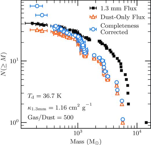
Comparison of cumulative clump mass functions from 1.3-mm maps (black squares), observed dust-only maps (orange triangles), and completeness-corrected dust-only maps (blue circles). The parameters used to convert the flux to gas mass in equation (7) are shown in the bottom left. Error bars are random uncertainties on clump masses from noise in the maps; see Section 3.3 for details.
3.4 Completeness corrections
We estimated the completeness of our mass function through Monte Carlo techniques by injecting synthetic sources of known fluxes and sizes into the dust-only maps one source at a time. We ran ClumpFind on the altered map with the same parameters as for the original maps and counted when synthetic clumps were recovered and when they were not. We then took the ratio of the number recovered to the total number injected as the completeness fraction. Synthetic source positions were randomly placed across the maps with a uniform distribution. All sources were elliptical Gaussians with FWHM and position angle identical to those of the synthesized beam for the corresponding map. We injected 600 synthetic sources per mass bin. Synthetic source masses were spaced evenly in log-space from roughly 21 to 1.2 × 10⁴ |$\mathrm{M}_{\odot}$|. Fig. 5 shows the completeness data for 30 Dor-10, N159W and N159E.
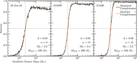
Completeness curves for point sources in 30 Dor-10, N159W and N159E (black line). The best-fit logistic curves (equation 8) are shown as orange dashed lines, with the best-fit parameters in the bottom right. 50 per cent completeness is marked by the vertical gray lines and reported as |$M_{50\%}$| in the bottom right.
A surprising feature of the completeness curves shown in Fig. 5 is that none of the maps actually attains 100 per cent completeness. This is related to how crowded each map is: a synthetic source added to a crowded map may land on a real clump, such that ClumpFind does not find the synthetic clump. 30 Dor-10 is the most crowded map and has the lowest maximum completeness, while N159E is the least crowded and has nearly 100 per cent recovery at high masses. This trend shows that it is not only the noise and resolution that limit our ability to find clumps but also the crowdedness of our maps.
It is important to note that we tested source recovery only for sources that were the same size as the synthesized beam, while most of the clumps that we have identified are much larger than the synthesized beam. Choosing an optimal completeness treatment is a general challenge when studying these types of objects, because molecular clumps are intrinsically amorphous in shape and vary significantly in physical size. Because larger clumps of the same integrated flux density as smaller clumps have a lower S/N, our completeness estimates probably overestimate the total fraction of clumps recovered for a given mass. While more sophisticated methods could be employed (e.g. see appendix B of Könyves et al. 2015), having a simplistic estimate of the completeness is better than having no estimate.
We use the fits to the completeness data to correct the mass function numbers by calculating Ncorr = N(≥M)/f(M). We used the 30 Dor-10 completeness curve because it contributes the majority of the clumps in our mass function. Application of this completeness correction produces the mass function shown as blue circles in Fig. 4, which can be compared with the observed mass function shown as orange triangles.
4 MASS FUNCTIONS IN THE LMC AND MILKY WAY
4.1 LMC clump mass function
An empirical mass distribution is typically plotted as either a differential mass function or a cumulative mass function. A differential mass function is calculated by defining mass bins spanning the mass range of objects and counting the number of objects within each bin. This form allows for a simple Poissonian counting statistics approach to uncertainties for fitting, but the results can depend on the choice of bin widths and centres. A cumulative mass function avoids complications from binning because it is just an ordered tally of masses at or above a given object’s mass. The trade-off is that there is not a simple statistical approach for handling uncertainties for fitting.
Given our relatively small sample of clumps and the simple model, we carried out our fits with the standard non-linear Levenberg–Marquardt least-squares minimization (More 1977). To estimate fitting weights we followed the approach used by Reid & Wilson (2006a), which specifies the y-data uncertainties as the cumulative number N(≥M) for each clump. The best-fit double-power-law parameters are given in Table 5 for the mass function determined directly from the clump masses, along with two variations that attempt to account for incompleteness. The procedure and inputs for the fits are the same across all three variations.
Results of double-power-law and lognormal fits to the cumulative clump mass function for the Large Magellanic Cloud.
| αlow | αhigh | Mbreak | |$M_{0}\, ^{a}$| | σ | |
|---|---|---|---|---|---|
| Initial guess | −1.8 | −3.5 | 2500 | 7 | 1 |
| Observed mass function (MF) | |$-1.50^{+0.06}_{-0.05}$| | −3.3 ± 0.2 | 2200 ± 200 | |$7.22^{+0.06}_{-0.04}$| | |$0.86^{+0.03}_{-0.04}$| |
| Observed MF, M > 500 |$\mathrm{M}_{ \odot}$| only | |$-1.74^{+0.01}_{-0.1}$| | −3.3 ± 0.2 | |$2500^{+300}_{-100}$| | |$7.3^{+0.2}_{-0.1}$| | |$0.81^{+0.04}_{-0.06}$| |
| Completeness corrected MF | |$-1.76^{+0.04}_{-0.05}$| | −3.3 ± 0.2 | |$2500^{+300}_{-200}$| | 6.8 ± 0.2 | |$1.03^{+0.06}_{-0.08}$| |
Note. aexp (M0) is the central mass of the lognormal function from equation (10). So, for example, the fitted central mass of the observed mass function is exp (7.22) ≈ 1370 |$\mathrm{M}_{\odot}$|.
Given the form of the fitting function, there are uncertainties only in the x-values. To estimate the absolute uncertainties on the best-fit parameters we used Monte Carlo simulation, as in Reid & Wilson (2006a). This process involved generating 105 artificial mass functions and fitting each in the same way as the observed mass function. The artificial mass functions were made by drawing normally distributed random deviates centred on each measured clump mass and with standard deviations equal to the measurement uncertainties on the masses from the dust-only maps. Each newly generated sample of 32 masses was then sorted into descending order to prepare for fitting. Not only does this Monte Carlo approach simplify estimation of the fit parameter uncertainties but it also nicely includes the effects of neighbouring masses swapping places in the sorted order as a result of their uncertainties. From the distributions of fit parameters, we used the inner 68 per cent to obtain the 1σ uncertainties on each fit parameter (Table 5).
Fig. 6 shows the completeness-corrected mass function with the best-fit double power law (Table 5). We used all the clumps in our sample in this fitting, with our lowest mass of 205 |$\mathrm{M}_{\odot}$| at the 41 per cent complete level. We also tested restricting the fit to masses above 500 |$\mathrm{M}_{\odot}$| in the uncorrected mass function, because this is roughly where the 30 Dor-10 completeness curve flattens out at maximum completeness. The best-fit double power laws for the two methods end up being statistically indistinguishable based on our Monte Carlo uncertainty estimates (Table 5), so we focus our analysis on the completeness-corrected mass function.
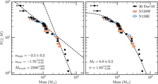
Completeness-corrected clump mass function (all points are the same as the blue circles in Fig. 4 but now with the originating source indicated), with best fits plotted as black dashed lines; the double power law is on the left and the lognormal function is on the right. Parameters of the fits (equations 9 and 10) are shown in the bottom left corners. Clumps are colour-coded by the region from which they originate, with 30 Dor-10 as black squares, N159W as orange triangles, and N159E as blue circles. Error bars are the same as in Fig. 4.
It may appear unusual that the numbers of high-mass clumps need to be boosted by our completeness correction. An overlapping pair of sources (merged clumps) would be identified in the data as a more massive clump and thus not be missed. We tested removing the completeness correction to the high-mass clumps by stitching together two sigmoid curves (the fit shown in Fig. 5 and a curve with the same width parameter but an amplitude of 1.0 and shifted slightly to higher masses) to create a smoothly varying sigmoid matching our measured completeness at low masses and asymptoting to 100 per cent complete at high masses. Refitting the mass function corrected with this piecewise completeness curve did steepen both indices and it moved the break to a higher mass, but all within the uncertainties of our original fit.
4.2 Comparison with other studies
The sample of 11 core/clump mass functions from seven distinct star-forming regions analysed by Reid & Wilson (2006b) is a useful one for comparing our LMC clump mass function with Milky Way mass functions. All mass functions were re-calculated from the original literature sources and fitted with a double power law (equation 9) homogeneously across all regions. While there are various differences in how those data were acquired and processed as well as in how individual cores and clumps were identified, the use of the best-fit parameters reported by Reid & Wilson (2006b) will remove any variability introduced in the fitting step. Fig. 7 compares the high- and low-mass slopes from Reid & Wilson (2006b) with our fit from Section 4.1 for the LMC.

Comparison of the double-power-law mass function fits from the seven Galactic star-forming regions summarized in Reid & Wilson (2006b) with the low- and high-mass fit indices for our Large Magellanic Cloud (LMC) mass function. Circles and triangles show the Galactic low- and high-mass indices, respectively. The orange and blue dashed lines and shaded regions show the low- and high-mass indices for the LMC, respectively. Milky Way clouds are arranged with their median core/clump masses increasing to the right. Open triangles denote less robust high-mass slope determinations for Galactic clouds M8 (clumps identified by eye) and M17 (mass function fit better with the lognormal function).
The LMC break mass is greater than the individual clump masses for all of the Milky Way objects except for W43 and RCW 106 (and greater than all Milky Way break masses, which range from 0.2 ± 0.1 to 400 ± 300 |$\mathrm{M}_{\odot}$|). As a result, it is probably more reasonable to compare the LMC low-mass slope with the high-mass slopes of the Galactic clouds. Fig. 7 shows that high-mass indices for ρ Oph at 850 |$\mu$|m, NGC 7538 (measured at both 450 and 850 |$\mu$|m) and W43 are consistent with the low-mass index for the LMC. All low-mass Galactic indices, except for Orion B from Motte et al. (2001), are systematically shallower than the LMC low-mass index. The observed consistency between the LMC low-mass index and the high-mass indices from ρ Oph, NGC 7538 and W43 suggests that the shape of the mass function may extend smoothly from the lower-mass clumps of the Milky Way regions to the higher-mass clumps of the LMC. In other words, it appears that the mass function slopes at high masses in the Milky Way extend up to the masses at the bottom of our LMC mass function.
In addition, none of the Galactic mass functions had completeness corrections applied and they are all probably suffering from incompleteness at their low-mass ends. Limiting our comparison to the high-mass end of the Galactic mass functions, where incompleteness should naturalli have a minimal effect, gives a fairer comparison with our LMC mass function because the completeness correction should ensure the effect of incompleteness is also minimized.
We note that there are four measurements of Galactic high-mass indices that are consistent with our high-mass index. Orion B as measured by both Motte et al. (2001) and Johnstone et al. (2001) is consistent within the uncertainties, despite values that are about 20 per cent shallower than ours, because the indices have uncertainties of almost 25 per cent. The remaining fields whose high-mass indices matches ours, M8 and M17, have large enough differences in analysis that we do not believe they present an issue for our conclusions. The cores from M8 were identified by eye rather than algorithmically as well as being fitted with an assumed Gaussian profile, unlike most of the other clump-finding procedures, including our own. For M17, the mass functions were either fitted as well as or better by a lognormal form, so it may not be a fair comparison with our mass function if the M17 mass distributions are not well characterized by a double power law.
The break masses from the Milky Way regions are all significantly smaller than the best-fit break mass for the LMC. Galactic break masses range from 0.2 ± 0.1 to 400 ± 300 |$\mathrm{M}_{\odot}$|. These differences are not surprising, as Reid et al. (2010) showed a correlation between distance and break mass using mass functions derived from synthetic observations of a simulated GMC. This trend can even be seen among the 11 mass functions from Reid & Wilson (2006b), as the break masses increase in step with decreasing spatial resolution. Our results for the break mass in the LMC are reasonable, given the much greater distance to the clumps.
Fig. 8 shows this comparison in another way. All Milky Way mass functions are reproduced from Reid & Wilson (2006b), while the LMC mass function is scaled such that the lowest mass (205 |$\mathrm{M}_{\odot}$|) is equal to the median maximum Milky Way mass (120 |$\mathrm{M}_{\odot}$|) and the lowest mass has N(≥M) = 1. Although this scaling is rather arbitrary, it illustrates the potential connection of the mass function shape between the lower masses in the Milky Way and the higher masses in the LMC.
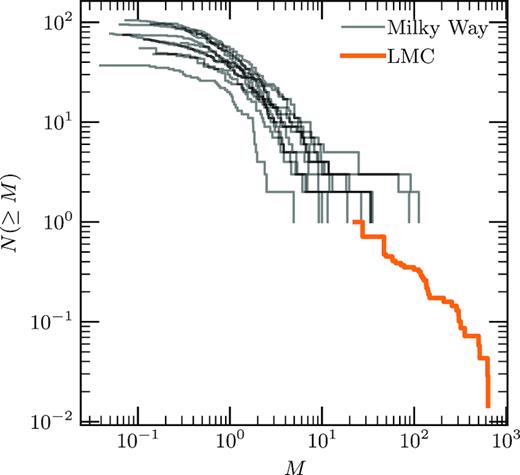
All Milky Way mass functions described in Reid & Wilson (2006b) reproduced from their fig. 8 in grey. The LMC mass function, in orange, has been normalized such that the lowest-mass clump is equal to the median of the maximum masses from the Galactic mass functions, and N(≥M) has been normalized such that the lowest mass has N(≥M) = 1.
Other recent observations have also measured the mass function of cores and clumps in the Milky Way. Netterfield et al. (2009) observed 50 square degrees of the Galactic plane in Vela with the balloon-borne large-aperture submillimetre telescope (BLAST) and fitted cold cores (<14 K) with a power law of –3.22 ± 0.14 and warmer cores with an index of −1.95 ± 0.05. A total of 738 cores were extracted from Herschel Gould Belt Survey observations of Aquila by Könyves et al. (2015). These authors fitted their mass function with an index of −2.33 ± 0.06, but after applying an age correction to the distribution they fitted an index of −2.0 ± 0.2. Pattle et al. (2017) observed the Cepheus flare region with SCUBA-2, which included four molecular clouds, namely L1147/L1158, L1174, L1251 and L1228. Individual power-law fits gave indices of −1.8 ± 0.2, −2.0 ± 0.2, −1.8 ± 0.1 and −2.3 ± 0.3, respectively, while fitting all regions together with a double power law gave a low-mass index of −1.9 ± 0.1 and a high-mass index of −2.6 ± 0.3. These results are in line with our conclusion that the high-mass Milky Way mass function slope is similar to the low-mass LMC slope, except when the entire Cepheus flare region is analysed together.
Another interesting comparison we can make is to the clump mass function for 30 Dor-10 derived by Indebetouw et al. (2013) using 13CO (2–1) and 12CO (2–1) data. Their single power-law fit to the differential logarithmic mass distribution of CO clumps above 500 |$\mathrm{M}_{\odot}$| resulted in a slope of α = −1.9 ± 0.2, which is consistent with the low-mass index measured from dust masses in this work. Fitting the differential form of the mass function resulted in only about five bins, two of which only have one or two clumps, so it is reasonable that the bins below our break mass would dominate their fit. The similar mass range between our dust-estimated masses and their independent CO-estimated masses is evidence for the accuracy of our dust-only map generation and our estimated dust properties.
Reid & Wilson (2006b) also presented lognormal fits to the Galactic mass functions listed in Fig. 7. The Milky Way values for M0 are all significantly lower than the LMC value, with only RCW 106 coming within ∼2σ, but this is expected because M0 is correlated with the mass function median mass similarly to the correlation between M0 and the double-power-law break mass. We find agreement in the LMC σ value and six of the Galactic mass functions. Both the ρ Oph measurements, and M8 and NGC 7538 measured at 850 |$\mu$|m show significantly different best-fit values for σ.
We can also search for a link between the LMC clump mass function and the mass distribution of groups of stars as they are first formed. The slope of −2 for young clusters measured by Lada & Lada (2003) is quite similar to our low-mass slope over a similar mass range. Analogous to how the similar shape of core mass functions and the stellar IMF has been posited as indicating a constant star-formation efficiency, the similarity of the clump and cluster mass functions may result from a constant cluster formation efficiency.
However, dust obscuration challenges observational measurements of the youngest, most deeply embedded star clusters. This hinders our ability to fully constrain the initial mass distribution of clusters when their stars are first born. Cluster formation simulations can bridge the gap between starless molecular clumps and the first star clusters as they emerge from their natal molecular clouds. Fujii & Portegies Zwart (2015) used a hydrodynamical simulation of the parent GMC, and after about a free-fall time instantaneously removed the gas and continued a solely N-body simulation of the stars formed. They measured mass function indices of −1.73 at 2 Myr and of −1.67 at 10 Myr for a range of initial GMC masses from 4 × 10⁴ to 5 × 10⁶ |$\mathrm{M}_{\odot}$|. Howard, Pudritz & Harris (2017) aimed to simulate cluster formation with the inclusion of radiative feedback in their hydrodynamical simulations in order to study its impact on cluster-forming efficiency. Starting from GMCs of similar masses to in Fujii & Portegies Zwart (2015), they found a close agreement between their simulated mass function power-law index of −1.99 ± 0.14 and observed embedded clusters. This was after 5 Myr and for masses from 10 to 2000 |$\mathrm{M}_{\odot}$|. For clusters >2000 |$\mathrm{M}_{\odot}$|, they fitted a steeper power law of index −3.8. These theoretical results are broadly consistent with the LMC clump mass function presented here.
5 CONCLUSIONS
We have presented a clump mass function measured in continuum dust emission from star-forming molecular clouds in the LMC derived from public archival ALMA observations. A total of 32 clumps were observed in the 30 Dor-10, N159W and N159E regions, with masses ranging between 205 |$\mathrm{M}_{\odot}$| and 5740 |$\mathrm{M}_{\odot}$|. In order to derive these total masses from the thermal dust emission we presented a technique of combining 3.2- and 1.3-mm maps to remove free–free emission contamination and produce dust-only emission maps. We implemented a point-source completeness correction to the clump numbers to account for the sensitivity and finite resolution of the observations
From our clump mass function we derived a double-power-law best fit with parameters |$\alpha _{\mathrm{low}} = -1.76^{+0.04}_{-0.05}$|, αhigh = −3.3 ± 0.2, and |$M_{\mathrm{break}} = 2500^{+300}_{-200} \ \mathrm{M}_{\odot }$|. Our low-mass power-law index is similar to the high-mass indices of Milky Way regions hosting lower-mass cores and clumps. This may indicate an extension of the Milky Way power law to higher masses. The addition of more clumps from more regions in the LMC, along with mass functions derived from spectral line emission, will be necessary to better characterize the mass distribution of these objects in the LMC and to investigate its consistency with the Milky Way mass functions.
ACKNOWLEDGEMENTS
We thank the anonymous referee for detailed comments that improved the content of this paper. This paper makes use of the following ALMA data:
ADS/JAO.ALMA#2011.0.00471.S,
ADS/JAO.ALMA#2012.1.00554.S,
ADS/JAO.ALMA#2012.1.00603.S,
ADS/JAO.ALMA#2013.1.00832.S,
ADS/JAO.ALMA#2013.1.01091.S,
ADS/JAO.ALMA#2013.1.01136.S, and
ADS/JAO.ALMA#2016.1.01533.S.
ALMA is a partnership of ESO (representing its member states), NSF (USA) and NINS (Japan), together with NRC (Canada), MOST and ASIAA (Taiwan), and KASI (Republic of Korea), in cooperation with the Republic of Chile. The Joint ALMA Observatory is operated by ESO, AUI/NRAO and NAOJ. The National Radio Astronomy Observatory is a facility of the National Science Foundation operated under cooperative agreement by Associated Universities, Inc. This research has made use of NASA’s Astrophysics Data System Bibliographic Services. This research made use of Astropy, a community-developed core Python package for Astronomy (Astropy Collaboration, 2013). This research made use of APLpy, an open-source plotting package for Python (Robitaille & Bressert 2012). This research has made use of the AstroBetter blog and wiki. CDW acknowledges financial support from the Canada Council for the Arts through a Killam Research Fellowship. The research of CDW is supported by grants from the Natural Sciences and Engineering Research Council of Canada and the Canada Research Chairs program.
Footnotes
All versions of casa were downloaded from https://casa.nrao.edu/casa_obtaining.shtml.
Note that after this paper was submitted, North American ALMA Science Center (NAASC) memo 117 was released detailing a problem with the flux scaling in 7-m ALMA mosaics imaged in versions of the casa software prior to 5.0. We have measured the differences in clump fluxes between the 30 Dor-10 maps presented here and ones produced with casa version 5.4.0-68 and find that, on average, the Band 6 flux densities are overestimated by ∼8 per cent and the Band 3 flux densities by ∼2 per cent. These small corrections have not been applied to the data presented in this paper.
A full code listing of the auto-masking algorithm is available in appendix B of Nathan Brunetti’s MSc thesis at https://macsphere.mcmaster.ca/handle/11375/22656.
Also see Dan Briggs’ PhD thesis at http://www.aoc.nrao.edu/dissertations/dbriggs/ for the full details of the weighting scheme and for more information on the ‘robust’ parameter.
The starlink software (Currie et al. 2014) is currently supported by the East Asian Observatory.
REFERENCES
APPENDIX A: OBSERVED, DUST-ONLY, AND FREE–FREE-ONLY MAPS
Figs A1 to A3 show all maps produced for 30 Dor-10, N159W and N159E in this work. The top rows show the observed maps, the middle rows show the free–free-only emission maps, and the bottom rows show the dust-only emission maps. The left columns are maps in Band 3, and the right columns are maps in Band 6. All maps are presented with the same spatial and colour axes scaling and ranges to facilitate comparisons between the morphologies of the different bands and emission sources.
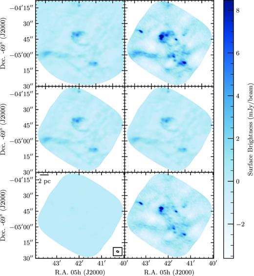
Maps of 30 Dor-10 in the 3.2-mm (left column) and 1.3-mm (right column) continuum, along with maps of free–free-only (middle row) and dust-only (bottom row) emission at both wavelengths. Spatial and colour coordinate axes are matched between each map. The uv-coverage of each map has been matched, and the synthesized beam shape is represented by the ellipse in the bottom-left panel.
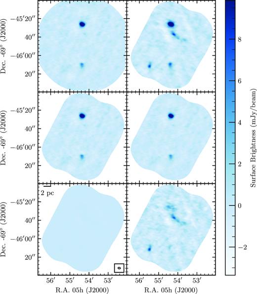
As Fig. A1, but for observations of N159W.
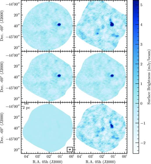
As Fig. A1, but for observations of N159E.
30 Dor-10 exhibits its strongest emission in Band 6, with compact dust sources accounting for most of the flux. N159W and N159E show similar levels of emission in the two bands, owing to the fact that most of the light comes from free–free emission, which slowly varies with frequency. All three fields show a gradual change in free–free brightness between Band 3 and Band 6, and a much stronger drop in dust emission when going from higher to lower frequencies.
