


ABSTRACT
We investigate the evolution of the radial distribution of blue straggler stars through a set of Monte Carlo simulations of star clusters under a variety of initial conditions. We used a novel technique based on the ‘artificial oversampling’ of the distribution function of the blue stragglers and control population to tear down the effect of statistical fluctuations affecting the determination of the relative distribution of these stellar populations. We find that a bimodal distribution, qualitatively similar but much less pronounced than those observed in many globular clusters, can naturally emerge as a result of the progressive migration of blue stragglers in the energy domain. The behaviour of the parameter A+, proposed as a ‘dynamical age’ indicator, has been also investigated. This parameter shows a relatively homogeneous and well-defined trend with the fraction of the elapsed core-collapse time-scale up to the core-collapse phase, while after this stage its evolution depends on initial conditions.
1 INTRODUCTION
The dynamical evolution of globular clusters (GCs) is a complex topic determined by the interplay of several physical processes such as stellar evolution, stellar collisions, tidal interactions, etc. Although the origin of GCs is still controversial (Peebles & Dicke 1968; Fall & Rees 1985; D’Ercole et al. 2008), the major milestones of their dynamical evolution have been largely studied through several kinds of dynamical simulations (Hénon 1971; Cohn, Hut & Wise 1989; Gao et al. 1991; Giersz & Spurzem 2003; Fregeau & Rasio 2007; Trenti, Heggie & Hut 2007).
On the other hand, from the observational point of view, we can only derive information on the present-day structure and kinematics of a given GC observing a snapshot of its entire evolution. For this reason, in the past years an important effort has been put in the search for an indicator of the stage of dynamical evolution of a GC acting as a ‘clock’.
As the main process at work during GC evolution is the two-body relaxation, all the indicators proposed so far are based on the effect left by this process on the main GC observables. In particular, interactions lead to a tendency towards kinetic energy equipartition with the most massive stars sinking in less-energetic (inner) orbits with respect to low-mass stars. As indicators of mass segregation, the comparison of the mass function slopes estimated at different radii (Webb & Vesperini 2017) and the variation of the velocity dispersion as a function of mass (Bianchini et al. 2018) have been proposed.
In a series of papers, the Bologna University group proposed that a special class of stars, the so-called blue straggler stars (BSS) could be used to trace the internal dynamical evolution of clusters (see Ferraro et al. 1999, 2006, 2009; Raso et al. 2017; Ferraro et al. 2018). This peculiar population of stars has been observed in the colour–magnitude diagram of all GCs at magnitudes brighter than the main-sequence turn-off, mimicking the presence of a population of young massive stars. The main hypothesis for the origin of these stars implies that they are the result of mass-transfer occurring in primordial binaries (McCrea 1964) or in stellar collisions (Hills & Day 1976). Aside from their formation process, BSS are thought to be three to four times more massive than the average mass (<m > = 0.3−0.4 M⊙) of stars populating old stellar systems such as Galactic GCs and for this reason have been suggested to be suitable gravitational probes to explore the degree of mass segregation in these stellar systems. In particular, in order to study the BSS radial distribution Ferraro et al. (1993) compared the fraction of BSS with respect to a reference population (usually horizontal branch or red giant branch (RGB) stars; NBSS/Ncon) and normalized to the fraction of cluster integrated light sampled in the same bin (RBSS).
The radial distribution of BSS has been found multimodal with at least three different morphologies: (i)Family I – flat distribution: BSS are distributed following the cluster light with RBSS = 1 at any distance from the cluster centre (Ferraro et al. 2006; Dalessandro et al. 2008); (ii)Family II – bimodal distribution: with a central overdensity of BSS followed by a dip at intermediate radii and an increase at large distances (Ferraro et al. 1997, 2004); (iii)Family III – unimodal distribution: with a central peak and a monotonic decreasing at larger distance (Contreras Ramos et al. 2012). The physical interpretation of such variety of morphologies has been provided by Ferraro et al. (2012; see also Mapelli et al. 2006) who proposed that the different observed morphologies are due to the radial dependence of the dynamical friction time-scale producing a progressive migration of BSS towards the GC centre and depriving regions at larger distance with increasing time. In this scenario, the location of the minimum (Rmin) in the RBSS radial distribution turns out as an indicator of the completion of the BSS sedimentation process.
However, this indicator has two major drawbacks: (i) it requires to bin the radial extent of data with a consequent degree of arbitrariety, and (ii) even the most massive GCs host only a few hundreds of BSS (Ferraro et al. 2006), thus it suffers from a large statistical noise.
Moreover, while the observational evidence of the BSS bimodal distribution is apparent in many GCs, its presence and prominence are less apparent in simulations. The first attempt in detecting such a feature in an N-body simulation has been made by Miocchi et al. (2015), who confirmed the general picture suggested by Ferraro et al. (2012): the formation of a sharp central peak, the development of a small dip ((NBSS/NRGB)min ∼ 0.9(NBSS/NRGB)tot) in the radial distribution, and the evolution towards a monotonic distribution at advanced stages. However, the detection of the bimodal distribution turned out to be quite noisy and the migration of the minimum towards large distance from the cluster centre was difficult to be followed. Similar difficulties have been found by Hypki & Giersz (2017) who analysed several Monte Carlo simulations of GCs under different initial and environmental condition. They found that while the BSS always segregate into the central regions of the GC, the increasing trend at large distances has been found as an unstable feature that also depends on the adopted binning.
In order to provide a more easily observable indicator of the BSS sedimentation process, Lanzoni et al. (2016) defined the parameter A+ as the area between the normalized radial cumulative distribution of the BSS and a reference population. They found a significant correlation between A+ and the position of the minimum Rmin in the analysed GCs and a nice relation with their cluster central relaxation time. Ferraro et al. (2018) extended this study to 48 GC confirming the correlation between A+ and the number of elapsed central relaxation times, thus suggesting the parameter A+ as a powerful dynamical age indicator. Alessandrini et al. (2016) tested the validity of this indicator in a set of N-body simulations run in idealized conditions (without binaries and stellar evolution and assuming BSS as single massive test particles) and found a good correlation between the A+ parameter and the fraction of elapsed core-collapse time (t/tcc).
Note that the simulations by Hypki & Giersz (2017), Miocchi et al. (2015), and Alessandrini et al. (2016) draw their conclusions using a realistic sample of only ∼100 BSS per simulation. Indeed, in a real GC BSS constitute only a tiny fraction of the GC mass, so that any improper oversampling of the BSS population in a simulation would bias its predictions.
In this paper, we investigate the radial distribution of BSS adopting a novel technique to overcome the problem of the low statistics. In Section 2, we discuss the concept of ‘dynamical age’ and provide our working definitions. In Section 3, the technique of artificial distribution function oversampling and its application to our Monte Carlo code is introduced. Section 4 is devoted to the description of the performed simulations. The resulting radial distributions of BSS is presented in Section 5. In Section 6, we discuss the effectiveness of the Rmin and A+ parameters in measuring cluster dynamical evolution. We summarize and discuss our conclusions in Section 7.
2 CONSIDERATIONS ON THE ‘DYNAMICAL CLOCK’
The search for parameters tracing the ‘dynamical age’ of a stellar system is triggered by the following question: ‘how advanced is the dynamical evolution of a stellar system?’. The above question, although crucial, could be misleading since different indicators can be advocated to trace different dynamical processes occurring over different time-scales affecting different regions of the cluster and all of them modifying the structural and kinematical parameters.
In particular, for a pressure-supported stellar system with an age comparable to or longer than its relaxation time, an initial phase of expansion (driven by the potential energy losses related to the evolution of massive stars in the first 108 yr; Chernoff & Weinberg 1990) is followed by a long period in which the large number of interactions between stars lead massive stars to release part of their kinetic energy to less massive ones, moving on inner orbits. As a result of this process, the mass function varies as a function of the distance from the centre and, in any given region of a GC, massive stars are kinematically colder than low mass ones (Spitzer 1969). At the same time, the large velocity acquired by low-mass stars makes them more prone to evaporation with a consequent flattening of the global mass function. Such a process can be accelerated by the interaction with the Galactic tidal field whose strength depends on the cluster orbit (Baumgardt & Makino 2003). The interplay between two-body relaxation and mass-loss leads to an instability of the core, which progressively loses kinetic energy and shrinks by more than an order of magnitude (core contraction and collapse; Larson 1970). The possible presence of binaries or heavy remnants (such as neutron stars and black holes; hereafter NS and BH, respectively) reduces the degree of mass segregation and can delay (or even halt and reverse) core collapse since these stars quickly sink into the cluster core and interact with other stars through three- and four-body encounters in which part of the binding energy of binaries is transferred into kinetic energy (Heggie 1975). These systems, because of their large mass, have low orbital energy and are therefore more efficiently retained with respect to single low-mass stars.
The efficiency and time-scale of the above processes depend in a complex way on the initial values of many parameters (i.e. mass-function, binary fraction and characteristics, cluster size and structure, orbit, etc.), which could have been different among GCs at their birth.
Moreover, processes such as kinetic energy equipartition and core collapse, while both being the outcome of the dynamical evolution, have efficiencies that depend on different parameters being therefore not univocally correlated, i.e. it is possible to find GCs close to core collapse whose stars have exchanged a lower fraction of their kinetic energy than those in a GC that is still far from this stage. So, although the general trend is towards high degrees of mass segregation, concentrated cores, large remnant fractions, none of the above observables univocally describe all the aspects of dynamical evolution.
For example, the problem of the dynamical cluster evolution can be put as follows: ‘the amount of changes in the structural and kinematical properties of a GC from their initial conditions’. This definition, while intuitive, is practically unaffordable. Indeed, at present, there is not a clear picture of the first stages of the GC life, where initial conditions are set. The proposed scenarios of GC formation involve a multiphase gas collapse forming multiple populations of stars characterized by different chemistry, structure, and kinematics (D’Ercole et al. 2008), the interaction of proto-GCs in gas-rich molecular clouds (Bekki 2017) and the possible presence of a primordial dark matter halo (Peebles & Dicke 1968). Besides this, it is unlikely that GCs form with universal initial conditions. Among the various parameters, many works suggested variations of the initial mass function (IMF; Marks & Kroupa 2010), initial size and concentration (Baumgardt et al. 2010), binary fraction (Sollima 2008), and degree of primordial mass segregation (Chen, de Grijs & Zhao 2007; McMillan, Vesperini & Portegies Zwart 2007), whose existence is under debate. It is therefore not obvious that a single (or a combination of) present-day observable can describe the amount of evolution of the same parameters in different GCs regardless of their unknown initial conditions.
3 METHOD
The simulations used in this paper were run using a modification of the Monte Carlo code presented in Sollima & Mastrobuono Battisti (2014). The general description of the orbit-averaged Monte Carlo method has been originally provided by Hénon (1971) and later developed by many authors (see e.g. Stodolkiewicz 1982; Giersz 1998; Joshi, Rasio & Portegies Zwart 2000). Briefly, the cluster is considered as a sample of N superstars characterized by their mass, energy, and angular momentum per unit mass that generates a spherical symmetric potential. At each time-step the following steps are performed:
a statistical realization of the cluster is performed by placing superstars at random positions along their orbits according to the time spent at that distance from the cluster centre,
each superstar is assumed to interact with its nearest neighbour producing a perturbation on their energies and angular momenta, and
the potential is evaluated according to the masses and positions of the superstars.
The above steps are repeated until the end of the simulation. The above scheme is efficient and versatile allowing to easily include many levels of complexity such as the presence of a mass spectrum (Giersz 2001; Joshi, Nave & Rasio 2001), the effects of stellar evolution (Chatterjee et al. 2010), three- and four-body interactions (Fregeau & Rasio 2007), and interaction with a tidal field (Sollima & Mastrobuono Battisti 2014). The effectiveness of the above technique in reproducing the effect of two-body relaxation in a wide range of initial conditions and environments has been widely tested against N-body simulations (see e.g. Hénon 1975; Giersz 2001; Joshi et al. 2001). A detailed description of the above steps is provided in Sollima & Mastrobuono Battisti (2014) and will not be repeated here. Next, we describe the modification to their code made to increase the statistics of BSS without biasing the result of simulations.
Each simulation is composed by three distinct samples: (i) a main sample constituted by 29 000 stars with different masses, fraction of binaries, and remnants, (ii) a BSS sample, constituted by 10 000 binaries whose evolution naturally drives towards BSS formation, and (iii) a control sample, constituted by 10 000 test particles with the mass of a typical RGB star in a GC (M = 0.83 M⊙). To define the BSS sample, we considered the formation scenario proposed by McCrea (1964) in which BSS form as a result of the Roche lobe overflow occurring during the expansion of the primary component of a close binary after its hydrogen exhaustion. For this purpose, we simulated a large population of binaries (following the prescription described in Section 4) and extracted only those systems satisfying the following conditions: (i) a primary star with mass larger than the turn-off mass of an old (t = 12 Gyr) metal-poor ([Fe/H] = −1.3) α-enhanced isochrone (from the Dotter et al. 2008, data base), (ii) a primary star radius at the RGB tip larger than the volume-averaged Roche lobe radius, following the criterion of Lee & Nelson (1988), (iii) a total lifetime (primary + BSS) longer than 12 Gyr. The above criteria have been verified at each time-step to exclude binaries which, after a series of interactions, modified their characteristics and would not produce BSS. Particles in the main sample evolve independently of the other samples following the canonical steps described above. At each time-step, the particles of the BSS and control samples are ranked in distance and associated to the closest main sample particle. The perturbation in energy and angular momentum is calculated and applied only to the stars in the BSS and control samples.1 In this way, particles in the BSS and control samples feel the effect of interactions with the cluster population, but their presence does not affect the canonical evolution of the main sample. The possible occurrence of three- and four-body is also accounted for according to the adopted prescriptions for these kind of interactions (see next). Being subject to the same kind of interactions occurring with the same probability as their corresponding population in the main sample, BSS, and control samples share the same distribution in phase-space of their parent stars, while their sizes are much larger. This novel technique, hereafter referred as ‘artificial distribution function oversampling’, allows to model the evolution of a number of BSS and control sample particles that exceed by orders of magnitude those of real BSS and RGB stars, without affecting the conservation of energy and angular momentum of the entire simulation.2 As a consequence, the distribution function of BSS and control sample particles, and their corresponding radial distributions, can be sampled with thousands of objects, thus reducing statistical fluctuations. Of course, the relative fraction of BSS and control sample particle does not reflect the corresponding fraction of these objects in the main sample. Hence, only their phase-space distribution will be used to study the BSS radial segregation and to derive the ‘dynamical age’ indicators proposed in the literature, which are all based on the radial distribution of BSS independently on the size of the BSS and reference population samples. As a sanity check on the validity of the ‘artificial oversampling’ technique, we compared the number fraction and energy distribution of particles in the control sample and those in the main sample with a mass in the range 0.78 < M/M⊙ < 0.83 at each time-step of all the simulations performed here. These quantities indeed trace the evaporation rate and the efficiency of two-body relaxation, respectively, and the same trend must be found in the oversampled (control) and main samples in the same mass range. The above-defined number counts ratio remains constant during the simulations within the uncertainties, although in the last snapshots the Poisson noise due to the low number of particles in the main sample makes this ratio quite noisy and small deviations (|$\lt\! 20{{\ \rm per\ cent}}$|) can occur because of the slightly lower mean mass of particles in the main sample. Moreover, we also performed a Kolmogorov–Smirnov test on both the cumulative radial and energy distribution of control sample and main sample particles in the above-defined mass range in selected snapshots of each simulation. Again, we always find a probability |$\gt 95{{\ \rm per\ cent}}$| that the particles are drawn from the same distribution in both the radial and the energy domain. Unfortunately, the same test cannot be performed on BSS sample particles because only a handful of BSS is present in the main sample, thus hampering the significance of such a test.
4 DESCRIPTION OF SIMULATIONS
In principle, to properly simulate the outcome of the evolution of a GC at the present day, simulations should start with a wide mass spectrum, evolve for a Hubble time including the effects of stellar evolution, and then only their last snapshot should be analysed. However, this would require a huge number of simulations to sample different stages of dynamical evolution with a corresponding unaffordable computation time. We adopted a simplified approach in which stellar evolution recipes are applied to the initial set-up, passively evolving the GC stellar population until an age of 12 Gyr. Then, the Monte Carlo simulation is run with these updated initial conditions and without stellar evolution for an arbitrary long time. We halt our simulations after 10.5 initial half-mass relaxation times that correspond to the dissolution time of most of our simulations. In this way, each snapshot of the simulation can be considered as the outcome of a 12 Gyr long evolution of a GC in a different dynamical stage. Of course, this is a rough approximation because the effect of stellar evolution is diluted over the entire life of a real GC, slowly changing the extent of the mass spectrum and the evolution of single and binary stars. However, this approximation does not introduce any bias in the BSS radial distribution. Indeed, each BSS and its progenitor binary system have the same total mass and are therefore subject to the same dynamical evolution. So, since binaries are converted into BSS with the same efficiency at all radii, the timing of BSS formation is irrelevant for our purpose. Moreover, stellar evolution driven mass-loss mainly occurs in the first Gyr of evolution, and it is therefore not expected to be significant on the long-term evolution of the simulation (but see Contenta, Varri & Heggie 2015).
Stars were extracted from an IMF defined between 0.08 and 120 M⊙ and distributed in phase-space following a King (1966) distribution function. No primordial mass segregation is included. A population of primordial binaries has been also simulated by random pairing stars from the IMF and assuming the period and eccentricity distribution of Duquennoy & Mayor (1991). From the initial library of binaries, we retained only those whose corresponding semimajor axis is comprised between the Roche lobe overflow separation (Lee & Nelson 1988) and the hard–soft boundary (amax = Gm1m2/2〈m〉〈σ2〉; where m1 and m2 are the two components of the binary, and 〈σ2〉 is the square of the 3D velocity dispersion averaged over the entire cluster). The stellar evolution recipes of Kruijssen (2009) have been applied to both single and binary stars. We assume a 100 per cent retention fraction of white dwarfs and different retention efficiencies for NSs and BHs. The initial number of particles in the main sample is set to N = 29 000 in all simulations. The corresponding total mass of the system, after passive stellar evolution, turns out to be M ∼ 104 M⊙. The simulated GC moves on a circular orbit within a tidal field generated by a point-mass of MG = 1010 M⊙.
We run a set of simulations starting from different initial conditions. For all simulations, we adopted a half-mass radius rh = 6 pc and assumed a 100 per cent retention fraction for white dwarfs (resulting in an initial mass fraction of |$\mu _{\mathrm{ WD}}\equiv M_{\mathrm{ WD}}/M=24{{\ \rm per\ cent}}$|). We defined a reference simulation in which particles are extracted from a Kroupa (2002) IMF, distributed according to a King (1966) model with a central adimensional potential W0 = 5, a fraction of binaries |$f_{b}=5{{\ \rm per\ cent}}$|, no heavy remnants (μNS,BH = 0), and move at a distance of RG = 5 kpc from the point-mass galaxy. This implies a tidally filling (rt ∼ rJ) cluster at the beginning of the simulation. Then, we set the other simulations by changing one of the above parameter at time. The entire set of simulations is summarized in Table 1. To define the core-collapse time, we adopted the technique described in Trenti et al. (2007) who place this event at the time when a break in the core-concentration evolution becomes noticeable. This definition, while non-optimal in case of an extreme density contrast (see next), has been found to be adequate in most of our simulations, being able to define this stage of evolution even in simulations with a significant fraction of primordial binaries and immersed in a strong tidal field, which do not show a sharp transition in the core size evolution (see Section 2).
Initial conditions of our simulations.
Initial conditions of our simulations.
In Fig. 1, the evolution of the mass, the core concentration (defined as log(rh/rc)), the mass function slope α, the Roche lobe filling factor (defined as log(rh/rJ)), the fraction of remnants and binaries are shown for the entire set of simulations as a function of the initial half-mass relaxation time. In the above definitions, we adopted the core radius (rc) definition by Casertano & Hut (1985), and rJ is the Jacobi radius (King 1962). It can be seen that the various parameters evolve differently according to the initial conditions. For instance, the core concentration varies by an order of magnitude among the whole set of simulations. On the other hand, simulation w5rg10, at odds with all the other simulations, underfills its Roche lobe during its entire evolution thus retaining most of its mass and maintaining almost constant its global mass function. Instead, the heavy remnants present in simulation w5rg5bh quickly sink into the cluster core and act as an energy reservoir that accelerates the response of the core and lead to a general expansion of the system. Note that, because of the core radius definition adopted here (from Casertano & Hut 1985), in this last simulation the core is almost coincident with the region containing the entire BH population. This leads to the occurrence of core collapse at early epochs, while visible stars maintain a more extended distribution.
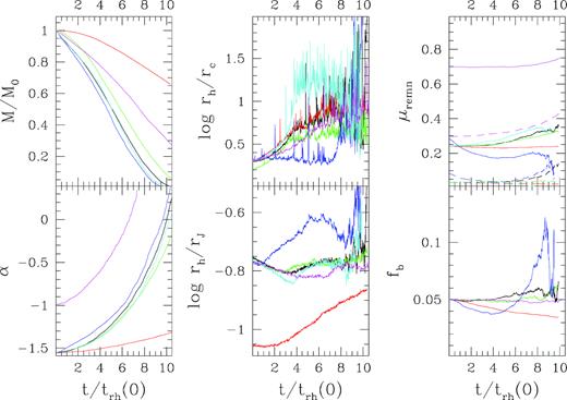
Evolution of the enclosed mass (top left-hand panels), mass function slope (bottom left-hand panels), core concentration (log(rc/rh); top central panels), Roche lobe filling factor (log(rh/rJ); bottom central panels), fraction of remnants (top right-hand panels; the total and massive (M > 0.83 M⊙). Remnant fractions are marked by the solid and dashed lines, respectively, and fraction of binaries (bottom right-hand panels). The behaviour of simulations w5rg5 (black lines), w5rg10 (red), w3rg5 (green), w5rg5bh (blue), w5rg5nobin (cyan), and w5rg5mf (magenta) is shown.
We show in Fig. 2 the comparison of the three dynamical time-scales (t/trh(t), S, and t/tcc) in all our simulations. It can be seen that, as discussed in Section 2, there is not a universal correspondence between these three indicators when different initial conditions are considered. In particular, the core collapse occurs significantly at smaller values of both t/trh(t) and S in simulation w5rg5bh (because of the early response of the core due to the kinetic energy injected by heavy remnants, see above) and w5rg10 (because of its longer relaxation time) than in the other ones. In the same way, the parameter S grows faster in simulation w5rg10 than in all the others subject to a strong tidal field. This occurs because simulation w5rg10 evolves almost in isolation and balances its slow mass-loss with an expansion keeping the half-mass relaxation time almost constant, while the other simulations are tidally limited (i.e. evolve at constant total density) and their half-mass relaxation time decrease with their mass. So, in the advanced stages of evolution of these simulations the instantaneous half-mass relaxation times is smaller than the its average value.
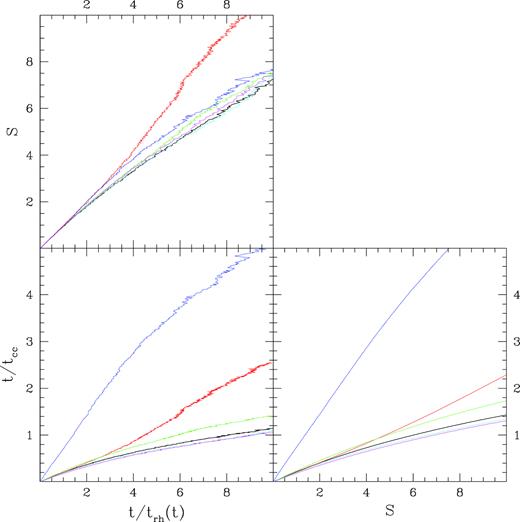
Comparison of the three dynamical time-scales t/trh(t), S, and t/tcc. The adopted colour code is the same as Fig. 1.
5 BSS RADIAL DISTRIBUTION
As a first analysis, we investigate the behaviour of the relative distribution of BSS and control sample particles in our simulations at different epochs, and compare it with what is observed in real GCs.
The normalized NBSS/Ncon ratio calculated in different stages of evolution is shown in Fig. 3 for simulation w5rg5 as a function of the projected distance from the cluster centre in units of both the core and the half-mass radius. The relative number of BSS shows a clearly defined behaviour and evolution: while at the beginning of the evolution it is almost flat (reflecting the absence of primordial mass segregation), a central peak develops whose intensity grows with time. This is the natural outcome of dynamical evolution since BSS, which are more massive than control sample stars, segregate into the cluster core in a time-scale comparable to the core relaxation time. At larger distances, the relative fraction of BSS has a minimum at NBSS/Ncon ∼ 0.8 and then slowly increases at increasing distances reaching again the primordial value close to the tidal radius. The BSS distribution remains bimodal during the following evolution being therefore a permanent feature, at odds with what found by Hypki & Giersz (2017).
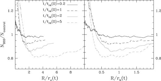
Normalized ratio of BSS and control sample particles in simulation w5rg5. The ratio is plotted both as a function of the core (left-hand panel) and the half-mass (right-hand panel) radius. Different lines indicate different stages of evolution. The typical uncertainties in this plot are <0.01.
To understand the physical reason of such a behaviour, we show in Fig. 4 the distribution of orbital energies (which together with the angular momenta determine the radial distribution of particles) of BSS and control sample particles in different stages of evolution. Note that while at the beginning the two populations are distributed in a similar way in the energy domain, as evolution proceeds BSS progressively migrate towards low energies (i.e. inner orbits) producing the central peak in the relative fraction. However, a significant fraction of BSS conserves their original energy creating a bimodal distribution, which reflects into the radial distribution. These BSS indeed spend most of their life in the peripheral region of the cluster, where the local relaxation time is longer than the cluster age, without interacting significantly with other cluster stars. This process is also enhanced by the presence of a mass spread in the BSS sample: the dynamical friction time-scale is indeed inversely proportional to mass, and massive BSS tend to sink into the cluster core faster than low mass ones. The same bimodal distribution is not apparent in the control sample particles because (i) their mass contrasts with respect to the other clusters stars smaller than that of BSS, and (ii) they do not contain a spread of masses.
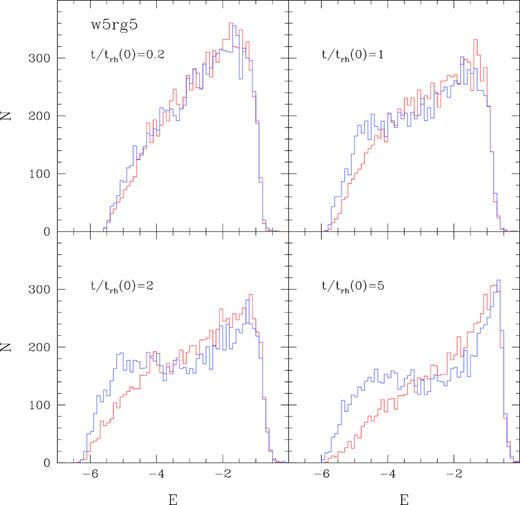
Distribution of orbital energies of BSS (blue histograms) and control (red histograms) sample particles in different snapshots of the w5rg5 simulation.
Fig. 3 shows that although the minimum of the distribution seems to be significantly less pronounced in the models considered here than that detected in the observations, its position, when expressed in units of core radii (Rmin/rc), appears to progressively migrate outwards. This migration is not evident in the right-hand panel when the radial position of the minimum is expressed in unit of the half mass radius Rmin/rh. This is visible in Fig. 5 where the evolution of Rmin is shown for simulation w5rg5. It is apparent that the behaviour of the minimum is quite noisy, and it is difficult to evaluate its decreasing rate at increasing time. In fact, the width of the region where the minimum is located increases with time making its exact localization difficult (Miocchi et al. 2015). As reference, the evolution of both rc and rh is also shown. From a qualitative comparison, the decreasing trend of the minimum appears to be more similar to that followed by the half-mass radius than to that of the core radius. This suggests that a negligible radial trend as a function of time should be expected when the RBSS distribution is plotted as a function of Rmin/rh, at odds with what is found in the observations (see Fig. 6) that show that the radial migration of the minimum is independent of the normalization of the radial coordinate. However, it is important to note that t/trh,0 is not known for the observed clusters in Fig. 6, nor is our suite of models aimed at reproducing their individual properties. Hence, further study is required to determine if the behaviour of Rmin/rh in our simulations is in disagreement with observations or just an artefact of the limited sample of observed clusters and/or the considered range of initial conditions in our simulations. It should be also noted that, at odds with simulations, observers usually estimate the core and half-mass radius through a fit of the surface brightness or star counts profile of the brightest population with some analytic model. This can introduce a time-dependent bias in the determination of these scale radii. To check the impact of such an uncertainty, we determined rc and rh in all the snapshots of simulation w5rg5 by fitting their projected density profile with a set of King (1966) models. For this purpose, in each snapshot the 3D positions of unevolved stars with mass |$M\,\,\gt\,\, 0.7\, \mathrm{ M}_{\odot }$| have been projected along one direction and their cumulative radial distribution have been compared with that of King (1966) models with different concentrations. The best-fitting model has been chosen as the one providing the best KS statistic. The rc and rh of the best-fitting models are overplotted to the actual ones in Fig. 5 as the red lines. It is apparent that both rc and rh estimated through the fit of bright stars decrease faster than their actual values until core collapse. However, also in this case, the decreasing trend of Rmin and rh still appears to be similar, at odds with what is shown by the observations in Fig. 6. Thus, this issue remains open.
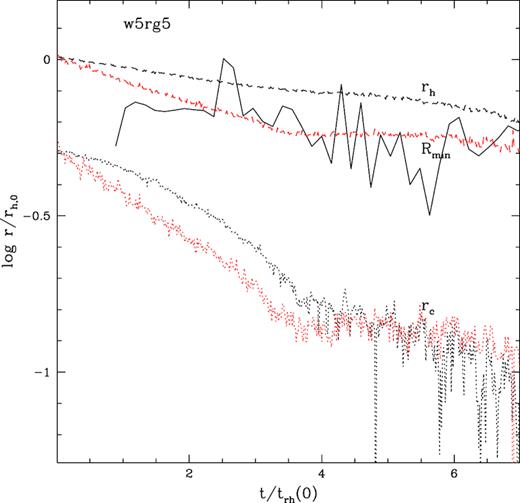
Evolution of the core, half-mass radius, and radius of the minimum of the BSS distribution in simulation w5rg5. The black lines indicate the rc defined as in Casertano & Hut (1985) (dotted lines) and the actual value of rh (dashed lines), while the red lines are the same radii estimated through the comparison with King (1966) models.
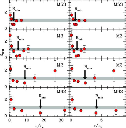
The normalized BSS radial distribution (red dots) for four clusters in the sample presented by Ferraro et al. (2012) are plotted as function of the distance from the cluster centre normalized to the core radius (left-hand panels) and the half-mass radius (right-hand panels). The grey strips schematically show the distribution of the reference populations. The thick arrows show the approximate location of the minimum of the distribution.
In Fig. 7, we compare the relative fraction of BSS and control sample particles as a function of distance predicted by different simulations. Note that although the height of the central peak varies in different simulations, the dip in the radial distribution is apparent in all of them but for the case of w5rg5bh. The heavy remnants present in this last simulation indeed dominate the core and interact with the BSS sunk into the core, thus reducing the effect of mass segregation. Note also that for simulation w3rg5 the bimodal distribution appears only after core collapse.
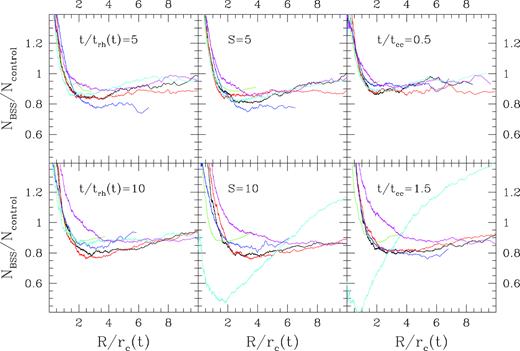
Comparison of the normalized ratio of BSS and control sample particles in our set of simulations. The distributions measured at two plotted in different values of t/trh(t) (left-hand panels), S (middle panels), and t/tcc (right-hand panels) are shown. The adopted colour code is the same as Fig. 1.
The bimodal behaviour of the relative fraction of BSS is qualitatively similar to that observed in real GCs by Ferraro et al. (2012). However, the minimum observed in many GCs reaches sometimes very low values (down to NBSS/Ncon ∼ 0.1; see their fig. 2) that are never reached in our simulations.
In order to investigate the effect of Poisson fluctuations, we calculated the radial profile of the relative fraction of BSS also from 104 random extractions of 100 BSS and 500 control particles. The result for the snapshot at t/trh(0) = 2 of simulation w5rg5 is shown in Fig. 8, where we highlighted in grey the region where 68 per cent of the extractions are located. We see that while no significant bias is apparent at any radius, the uncertanties in the population ratios can be significantly larger than those discussed above. A similar amount of noise is expected also in the simulations by Hypki & Giersz (2017) that contain samples of BSS and control stars of similar sizes. These fluctuations allow the detection of the growing trend of the relative fraction of BSS in only a fraction of the analysed snapshots, erroneously leading to the interpretation of this feature as transient. We also notice that the identification of the minimum in such condition is even more difficult, possibly producing false detection.
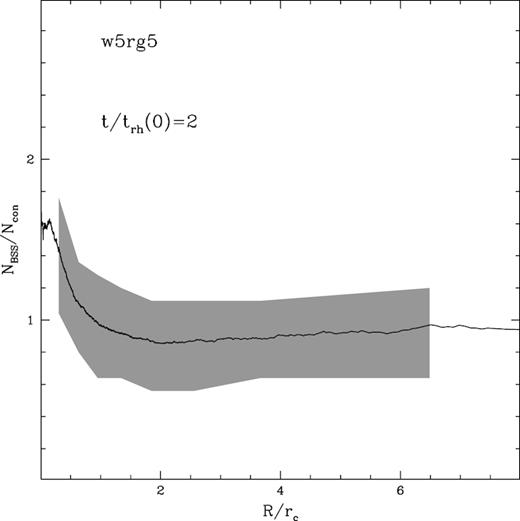
Relative fraction of BSS as a function of the projected distance for the snapshot at t/trh(0) = 2 of the simulation w5rg5 (solid line). The grey area indicates the region including 68 per cent of the measures performed in 104 random realizations.
It is worth noting that in our simulations we considered only BSS formed through the evolution of primordial binaries. In principle, a contribution to the BSS population could be also given by the collisions between single stars and by binaries. However, ‘collisional’ BSS are expected to form in the cluster centre and remain confined within the core during their entire evolution. So, this effect would increase the height of the central peak in the NBSS/Ncontrol ratio without affecting its radial trend outside the core.
6 BSS SEGREGATION INDICATORS AS ‘DYNAMICAL CLOCKS’
Once clarified the nature of the dip in the relative fraction of BSS, we investigated the behaviour of this feature, as well as the parameter A+, during the dynamical evolution of our simulations.
In principle, an ideal empirical ‘dynamical age’ indicator should (i) show a monotonic behaviour in terms of (at least) one the three time-scales defined in Section 2, and (ii) show a good level of independence on initial conditions. According to its definition (Alessandrini et al. 2016) and its recent applications (Lanzoni et al. 2016; Raso et al. 2017; Ferraro et al. 2018), the parameter A+ has been calculated as the area delimited by the normalized cumulative radial distributions of BSS and control particles, when the projected radial distances are expressed in logarithmic units. In Fig. 9, the evolution of the two considered parameters as a function of the three considered dynamical evolution time-scales is shown for all our simulations. The behaviour of Rmin/rc turns out to be quite noisy, even in our simulations where the number of BSS and control sample particles are oversampled by about two orders of magnitudes. Thus, in order to better delineate the overall trend of this parameter as a function of different dynamical time-scale, the best-fitting curves to the simulations and their 1σ spreads are plotted in the figure. As apparent, the parameter shows a generally increasing profile at early epoch with a decrease occurring in some simulations after core collapse. Moreover, as shown by Ferraro et al. (2012), highly dynamically evolved clusters show a unimodal BSS distribution, hence no minimum is expected to be detected in those clusters. This is also true for dynamically unevolved clusters, where the normalized BSS distribution is flat and again no minimum can be detected. All these limitations, combined with the intrinsic difficulties in detecting the minimum, use Rmin/rc as an indicator of dynamical age not optimal.
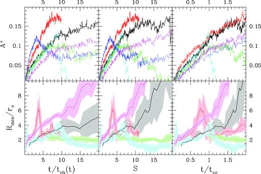
Evolution of the Rmin/rc (bottom panels) and A+ (top panels) parameters as a function of the three dynamical evolution time-scales defined in Section 2. t/trh(t) (left-hand panels), S (middle panels), and t/tcc (right-hand panels). The adopted colour code is the same as Fig. 1. In the bottom panels, the 1σ spread around the mean trend is marked by the shaded area. The simulation w5rg5bh (blue line), for which a unimodal distribution is found during its entire evolution, is not present in the bottom panels.
On the other hand, the A+ parameter shows a similar behaviour but with much more clear and well-defined trends. Indeed, this parameter monotonically grows with time until core collapse, while after this stage the behaviour of A+ significantly varies in simulations with different initial conditions. In particular, after core collapse the energy budget of the core (where most BSS reside) is supported by the interactions involving binaries. BSS, being more massive than other control sample particle, are more subject to such interactions and are scattered at large distances. This effect can produce a decrease of the mass segregation index A+ that is more prominent when more energetic interactions (like those occurring in simulation w5rg5nobin starting without primordial binaries) occur. Note also that while the evolutionary paths of A+ predicted by different simulations have a significant spread when expressed in units of t/trh(t) and S, a relatively small spread is apparent in terms of t/tcc for t < tcc. So, although the criteria defined at the beginning of this section are not strictly satisfied, the A+ parameter could be used as a proxy for the time needed to reach core collapse in those GCs who have still not experienced this event.
For comparison, in Fig. 10 the evolution of the A+ parameter is compared with that of the ‘kinematic concentration’ parameter (ck), which has been also proposed as an indicator of dynamical evolution by Bianchini et al. (2018). It can be seen that the kinematic concentration satisfies both the criteria defined above along the entire evolution of all our simulations. On the other hand, although observational uncertainties have not been simulated here, it is subject to a significant noise and can be considered independent on initial condition only when expressed in terms of t/trh(0) and S. Besides intrinsic fluctuations, part of the noise apparent in Fig. 10 is due to the low-number statistics and could be significantly reduced in observations of real GC. We note, however, that at odds with the indicators based on the radial distribution of BSS, the derivation of the ck parameter is observationally challenging because it requires the measure of velocities of stars in different mass regimes along the main sequence (a task that became feasible only recently; Bellini et al. 2014, 2018; Kamann et al. 2016, 2018), and the derivation of individual masses through the comparison with suitable stellar models.
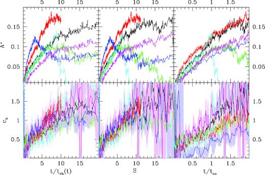
Evolution of the ck (bottom panels) and A+ (top panels) parameters as a function of the three defined dynamical time-scales t/trh(t) (left-hand panels), S (middle panels), and t/tcc (right-hand panels). The adopted colour code is the same as Fig. 1. In the bottom panels, the 1σ spread around the mean trend is marked by the shaded area.
For a quantitative analysis, we calculated the horizontal spread in the considered set of simulations in Figs 9 and 10 at specific values of Rmin/rc, A+, and ck in units of t/trh(t), S, and t/tcc. Although our simulations do not span the entire range of initial conditions covered by real GCs, these spreads can be considered as the typical uncertainty in the derived ‘dynamical age’ for each of the considered indicators. We chose as reference values Rmin/rc = 3, A+ = 0.07, and ck = 0.5, which roughly correspond to the values of these parameters in the reference simulation (w5rg5) at the time t/trh(0) = 2.2. The measured standard deviations and the maximum differences among the various simulations are listed in Table 2. It can be noted that, while indicators based on the radial distribution of BSS cover a range of several t/trh(t) and S, the kinematic concentration ck has a significantly smaller spread. On the other hand, in terms of t/tcc, the situation is reversed with A+ providing the smallest spread. This is somehow expected because of the different location of the tracers adopted by the above indicators: while the ck parameter is measured in terms of global quantities (and it is therefore well correlated with t/trh), those parameters based on the BSS radial distribution are more sensitive to the dynamical evolution of the core (and better correlated with t/tcc), where most BSS reside.
| Value | σ(t/trh(t)) | σ(S) | σ(t/tcc) | |
|---|---|---|---|---|
| Rmin/rc | 3 | 3.11 (7.7) | 2.02 (7.0) | 0.27 (1.7) |
| A+ | 0.07 | 1.88 (5.4) | 1.38 (4.0) | 0.21 (0.5) |
| ck | 0.5 | 0.67 (2.0) | 0.48 (1.4) | 0.35 (0.9) |
| Value | σ(t/trh(t)) | σ(S) | σ(t/tcc) | |
|---|---|---|---|---|
| Rmin/rc | 3 | 3.11 (7.7) | 2.02 (7.0) | 0.27 (1.7) |
| A+ | 0.07 | 1.88 (5.4) | 1.38 (4.0) | 0.21 (0.5) |
| ck | 0.5 | 0.67 (2.0) | 0.48 (1.4) | 0.35 (0.9) |
| Value | σ(t/trh(t)) | σ(S) | σ(t/tcc) | |
|---|---|---|---|---|
| Rmin/rc | 3 | 3.11 (7.7) | 2.02 (7.0) | 0.27 (1.7) |
| A+ | 0.07 | 1.88 (5.4) | 1.38 (4.0) | 0.21 (0.5) |
| ck | 0.5 | 0.67 (2.0) | 0.48 (1.4) | 0.35 (0.9) |
| Value | σ(t/trh(t)) | σ(S) | σ(t/tcc) | |
|---|---|---|---|---|
| Rmin/rc | 3 | 3.11 (7.7) | 2.02 (7.0) | 0.27 (1.7) |
| A+ | 0.07 | 1.88 (5.4) | 1.38 (4.0) | 0.21 (0.5) |
| ck | 0.5 | 0.67 (2.0) | 0.48 (1.4) | 0.35 (0.9) |
7 SUMMARY
Through a set of Monte Carlo simulations starting with different initial conditions (strength of the tidal field, concentration, binary and heavy remnant fraction, and mass function), we found that dynamical evolution can naturally reproduce a bimodal radial distribution of the BSS population. In particular, the presence of a dip quickly emerges in most simulation and remains visible along the entire simulation.
This feature is produced by the progressive migration of BSS in the energy domain determining a bimodal orbital energy distribution. A similar dip has been already identified in recent N-body and Monte Carlo (Miocchi et al. 2015; Hypki & Giersz 2017) simulations. In particular, Hypki & Giersz (2017) interpreted the discontinuous detection of this feature in subsequent snapshots of their simulations as an evidence of its transient nature. This is the first time that the significance and stability of this feature, is verified with a large set of Monte Carlo simulations. Indeed, while the N-body simulations of Miocchi et al. (2015) and Hypki & Giersz (2017) both contain three times more particles, they include only a small number of BSS that hamper the possibility to draw any firm conclusion on this issue. On the other hand, the artificial oversampling of the distribution function of BSS allowed us to determine the radial distribution of BSS with thousands of particles tearing down the effect of statistical fluctuations.
However, although such a feature is qualitatively similar to those observed in real GCs (see Ferraro et al. 2012), a few details remain not reproduced in the simulations. First, the migration of the position of the dip seems to be sensitive to the normalization radius (rc or rh) at odds with observations, where the position of the minimum follows the same evolution regardless of the radial normalization (see Fig. 6).
Secondly, the depth of the dip is less pronounced than what is found in the observations, as already found in the N-body and Monte Carlo simulations by Miocchi et al. (2015) and Hypki & Giersz (2017). While our simulations do not account for the effect of stellar evolution, simulate clusters with a mass that is more than one order of magnitude smaller than those of real GCs and cover only a small portion of the parameter space of initial conditions, it seems difficult to reproduce the almost complete lack of BSS at intermediate distances observed in many GCs (those belonging to the ‘Family II’ defined in Ferraro et al. 2012). Moreover, as demonstrated in Fig 8, when a realistic number of BSS and RGB stars are considered, the expected uncertainties in the measured normalized ratio are ∼1.5 times larger than the signal predicted by our simulations. So, if such a large uncertainties can explain the observed bimodal trend in some individual GC, this feature should not be easily observable in a large sample of GCs. In summary, although our simulations seem to identify the physical process leading to a bimodal BSS radial distribution, it is not clear if additional phenomena occurs making this feature as strong as observed in real GCs.
The behaviour of the Rmin/rc and A+ parameters (recently proposed by Alessandrini et al. 2016) has been also investigated and compared with that of the ‘kinematic concentration’ parameter proposed by Bianchini et al. (2018). The Rmin/rc appears to be extremely noisy also in our idealized simulations containing samples of thousands of BSS and control sample particles. On the other hand, if we restrict our analysis to the epoch preceding core collapse, the evolution of the A+ parameter shows a relatively small spread when expressed in terms of the core-collapse time (σ(t/tcc) ∼ 0.2) regardless of the initial conditions of the simulation. The same conclusion has been reached by Alessandrini et al. (2016) who, however, considered only N-body simulations without binaries and did not follow the post-core-collapse evolution.
Thus, although this parameter does not satisfy the general criteria defined above along the entire evolution, it could be considered a quite promising indicator of the evolution of a GC along its path towards core collapse at least during its pre-core-collapse phase. On the other hand, the ck parameter is found to be more effective in tracing the global relaxation of the cluster, while being less sensitive to the core evolution. These parameters provide therefore complementary information on the cluster overall dynamical evolution.
In the future, it will be interesting to verify whether the same behaviour is also seen in the observations. At the moment, the observational facts suggested that a negligible fraction of BSS is found in the external regions of post-core-collapse GCs and that the GC with the largest measured value of A+ (in a sample of 48 GCs; Ferraro et al. 2018) is indeed the post-core-collapse cluster NGC6397. In comparison with other indicators of dynamical evolution (defined as a function of global quantities and therefore sensitive to the general efficiency of two-body relaxation; Bianchini et al. 2018; Webb & Vesperini 2017), the A+ parameter is more sensitive to the process of relaxation occurring in the core where most BSS reside. All these indicators can be therefore used in a complementary way to study different aspects of the dynamical evolution of GCs.
It will be also interesting to investigate if differences in initial condition of the binary population possibly present at the formation of the GC stellar populations could possibly affect the long-term evolution of its BSS population. Indeed, any difference in initial condition of the binary population possibly present at the formation of the GC stellar populations could reflect on the long-term evolution of its BSS population. In this context, different binary fractions have been observed in Na-rich and Na-poor stars in several GCs (Lucatello et al. 2015) whose evolution could lead to bimodal trends in their radial relative fraction (Hong et al. 2015, 2016). However, the entire process of star formation in GCs occurs at early epochs (>1010 yr) and in a short time-scale (<108 yr Renzini 2008; D’Ercole et al. 2008), and it is therefore difficult that initial conditions have not been erased by two-body relaxation. In this respect, it would be interesting to investigate the evolution of the BSS population in GCs characterized by multiple episodes of early star formation. From the observational side, any possible link between the radial distribution of BSS and their chemical properties would be helpful.
ACKNOWLEDGEMENTS
We warmly thank Michele Bellazzini, Enrico Vesperini, and Anna Lisa Varri for useful discussions. We also thank the anonymous referee for his/her helpful comments and suggestions.
Footnotes
It is possible that in the same time-step two or more BSS and/or control particles interact with the same main sample particle. This, however, does not produce any inconsistency in the evolution of the energy and angular momentum distributions because main sample particles do not feel the presence of the other samples, and they provide only the statistical probability of interaction with a given cluster star.
Note that each BSS and control sample particle can interact only with a particle of the main sample, while BSS–BSS, control–control, and BSS–control interactions are forbidden. In this way, each particle of the BSS and control samples is an independent tracer of the distribution function of its population.
REFERENCES
