


ABSTRACT
We present the latest version of the ray-tracing simulation code skylens, which can be used to develop image simulations that reproduce strong lensing observations by any mass distribution with a high level of realism. Improvements of the code with respect to previous versions include the implementation of the multilens plane formalism, the use of denoised source galaxies from the Hubble eXtreme Deep Field, and the simulation of substructures in lensed arcs and images, based on a morphological analysis of bright nearby galaxies. skylens can simulate observations with virtually any telescope. We present examples of space- and ground-based observations of a galaxy cluster through the Wide Field Channel on the Advanced Camera for Surveys of the Hubble Space Telescope, the Near-Infrared Camera of the James Webb Space Telescope, the Wide Field Imager of the Wide Field Infrared Survey Telescope, the Hyper Suprime Camera of the Subaru telescope, and the Visible Imaging Channel of the Euclid space mission.
1 INTRODUCTION
The phenomenon of gravitational lensing is a direct consequence of the theory of general relativity, which relates the curvature of space–time to the distribution of matter and energy in the Universe. The images of distant sources will be magnified and distorted to different degrees depending on the amplitude of the mass concentrations and the relative geometrical configuration between the source, the deflectors encountered by light along its path, and observers on the Earth (Bartelmann & Schneider 2001; Treu 2010; Bartelmann & Maturi 2017). As such, gravitational lensing has become a fundamental tool to understand the nature of the dark matter and dark energy that, according to the current standard cosmological model, constitute 95 per cent of the total content of the Universe (Weinberg et al. 2013; Kilbinger 2015)
The most powerful gravitational lenses are galaxy clusters, since they are the most massive gravitationally bound structures in the universe. Thus, they act as cosmic telescopes, magnifying faint galaxies at high redshifts that contributed to the reionization of the early universe (Huang et al. 2016; Livermore, Finkelstein & Lotz 2017; Kelly et al. 2018). In the central regions of clusters, gravitational lensing can produce multiple images of the same source and elongated arcs. At larger angular distances from the cluster core, the individual tangential distortions induced on images are weak and therefore can only be detected statistically. The combination of these two regimes of gravitational lensing (known as strong and weak lensing, respectively) constrains the dark matter distribution from cluster centres to scales of up to 1 Mpc h−1, improving our understanding of the internal structure of galaxy clusters, and as a consequence, of the nature of dark matter and dark energy (Allen, Evrard & Mantz 2011). Upcoming future galaxy surveys will allow the automatic or semi-automatic detection of several gravitational arcs for a systematic study of a large population of cluster-scale lenses (Seidel & Bartelmann 2007; Stapelberg, Carrasco & Maturi 2017; Carrasco et al. 2018; Metcalf et al. 2018).
The measurement of the gravitational lensing signal to the level of precision required by current and future galaxy surveys has proven to be challenging. The characterization of sources of uncertainty such as systematic and modelling errors is crucial. The use of simulations with known inputs and different levels of realism has become a fundamental and standard tool to better understand these errors and validate measurement techniques and algorithms (Amara et al. 2006; Heymans et al. 2006; Kitching et al. 2013; Rowe et al. 2015; Li et al. 2016; Birrer & Amara 2018; Metcalf et al. 2018).
In this paper, we describe new developments and improvements of the gravitational lensing simulation pipeline skylens (Meneghetti et al. 2008, 2010) that can be used to create mock ground- and space-based observations of lensing phenomena by galaxy clusters and by large-scale structures in wide fields. Previous versions of skylens have been used to study the systematic errors in cluster mass measurements using lensing and X-ray analyses (Meneghetti et al. 2010; Rasia et al. 2012). skylens has also been used to construct synthetic lenses with the properties of the clusters observed by the Hubble Space Telescope (HST) in the Frontiers Field Initiative (Lotz 2015) in order to test the accuracy of inversion algorithms that reconstruct the cluster matter distributions from strong lensing measurements (Meneghetti et al. 2017). The improvements described in this work are aimed at increasing the realism of the simulations to make SkyLens an even more optimal tool in many applications of lensing by galaxy clusters.
The paper is organized as follows. In Section 2, we review our simulation pipeline and describe in detail the changes with respect to previous versions of the code. As an example of the output of the code, in Section 3 we use the current version of SkyLens to produce simulated observations through several astronomical instruments with realistic parameters and conditions: the Wide Field Channel (WFC) on the Advanced Camera for Surveys (ACS) of HST, the Near-Infrared Camera (NIRCam) of the James Webb Space Telescope (JWST), the Wide Field Imager (WFI) of the Wide Field Infrared Survey Telescope (WFIRST), the Hyper Suprime Camera (HSC) of the Subaru Telescope, and the Visible Imaging Channel (VIS) of the Euclid space mission. We discuss applications of SkyLens in Section 4, and conclude in Section 5. Unless otherwise noted, we assume a flat Λ cold dark matter (ΛCDM) cosmological model with a matter density parameter Ωm, 0 = 0.272 and a Hubble constant of H0 = 70.4 km s−1 Mpc−1.
2 SKYLENS
In this section, we describe skylens, highlighting the differences with respect to other versions (Meneghetti et al. 2008, 2010). The version of skylens presented in this paper includes the use of HST source galaxy images denoised by the method introduced in Maturi (2017). skylens now has the capability to include the lensing effects due to multiple lens planes. We also use information from a sample of nearby, well-resolved galaxies to produce realistic simulations of substructures such as regions of active star formation. We model these features as Sérsic (Sérsic 1963) profiles that will be magnified by the lens and appear as knots within the arcs that form at the critical lines in the lens plane. In addition, they can be used by lensing inversion algorithms as additional constraints that must satisfy the condition that they all must trace back to the same source, limiting the parameter space of solutions and increasing the likelihood of a more accurate model optimization in the source plane.
2.1 General methodology
For simulating an observation of a patch of the sky, with or without lensing effects, skylens goes through the following steps.
It generates a population of galaxies using the luminosity and the redshift distribution of the galaxies in the Hubble Ultra Deep Field (HUDF; Beckwith et al. 2006).
It prepares the virtual observation, receiving the pointing instructions, the exposure time, and the filter, F(λ), to be used from the user. The pointing coordinates are used to calculate the level of the background, i.e. the surface brightness of the sky and, in case of observations from the ground, the airmass.
- It assembles the virtual telescope. This implies that the user provides a set of input parameters, such as the effective diameter of the telescope, the field of view, the detector specifications [e.g. gain, readout noise (RON), dark current, and pixel scale], and the additional information necessary to construct the total throughput function, defined as(1)\begin{eqnarray*} T(\lambda)=C(\lambda)M(\lambda)R(\lambda)F(\lambda)A(\lambda). \end{eqnarray*}
In the previous formula, C(λ) is the quantum efficiency of the detector, M(λ) is the mirror reflectivity, R(λ) is the transmission curve of the lenses in the optical system, and A(λ) is the extinction function (galactic and atmospheric, in case of simulations of ground-based observations).
Using the spectral energy distributions (SEDs) and the redshifts of the galaxies entering the field of view, it calculates the fluxes in the band of the virtual observation. Then, using the galaxy templates, the surface brightness of the sources is calculated at each position in the sky and converted into a number of analog-to-digital units (ADUs) on the detector pixels.
Noise is added according to the sky brightness, to the RON, and to the dark current of the detector.
2.2 Denoised source image generation
Previous versions of skylens have used shapelets (Bernstein & Jarvis 2002; Refregier 2003) decomposition of HUDF galaxies to simulate a synthetic sky of source galaxies. The current version implements the technique introduced in Maturi (2017) (based on expectation maximization principal components analysis, EMPCA) to obtain a denoised (noise-free) reconstruction of images based on the Hubble eXtreme Deep Field (HXDF; Illingworth et al. 2013) data, which covers an area of 10.8 arcmin2 down to ∼30 AB magnitude (Rafelski et al. 2015).1 These images were taken by the ACS and the Wide Field Planetary Camera 2 in the F435W, F606W, F775W, F814W, and F850LP bands, and have been ‘drizzled’ to a resolution of 0.03 arcsec pixel−1. The SEDs of the source galaxies were obtained by interpolating the 11 SED templates from the photometric redshift measurements by Coe et al. (2006), as determined by the Bayesian photometric redshift code (Benítez 2000; Benítez et al. 2004).2 The Coe et al. (2006) library includes SEDs for elliptical, spiral (including starburst), and lenticular galaxies.
In Fig. 1, we show and example with two denoised galaxies (colour composite image and F775W band), together with the original HXDF image and the residuals. The bottom panel of the same figure shows a zoom-in of the source plane, without the additional substructures, used to produce the image of Fig. 7.
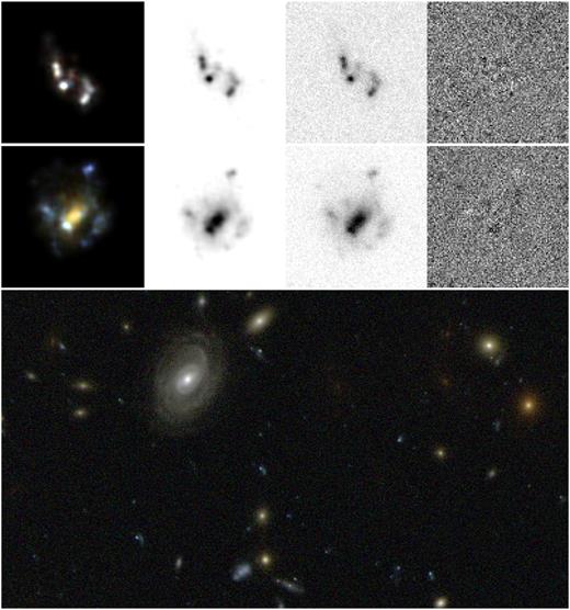
In the top two panels, we show two galaxies used to produce the source plane. From left to right: the colour composite image, the denoised image of the F775W band, the original HXDF image (with the other objects present in the postage stamp already removed), and the residuals. In the bottom panel, we show a cut-out of the source plane used to produce Fig. 7 but without the addition of the substructures.
2.3 Lens model
Shear, magnification (on the source and lens planes), and the locations of the caustic and critical lines are also readily derived from the deflection angles (e.g. Meneghetti et al. 2017).
2.4 Multiple lens planes
In Fig. 2, we show an example of multilens plane simulation. In the upper left-hand panel, we show the surface density map of the cluster Ares. The cluster is at redshift |$z$| = 0.5. We have extracted from a hydrodynamical simulation two slices of particles and we have used them to construct two additional lens planes at redshift |$z$| = 0.7 and |$z$| = 1. The details of the numerical simulation are in Meneghetti et al. (2010). The surface mass density on these two planes is shown in the second and third upper panels. Finally, we use the multilens plane formalism to compute the effective convergence for sources at |$z$| = 12, which is shown in the upper right-hand panel. Note that, in the effective convergence map, the mass structures behind the cluster appear distorted by lensing.
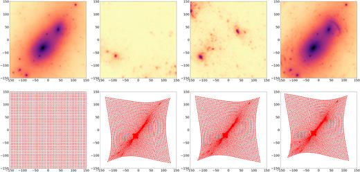
Example of multilens plane simulation. Upper panels: the left-hand panel shows the convergence map of the Ares cluster. In second and in the third panels we show two mass sheets extracted from a cosmological simulation at |$z$| = 0.7 and at |$z$| = 1. We use the multiplane ray-tracing technique to propagate light rays up to |$z$| = 12 (fourth panel). The resulting effective deflection angles are used to compute a map of the effective convergence shown in the left-hand panel. Bottom panels: in the leftmost panel, we show the regular grid through which we propagate the light rays on the first lens plane. In the other panels, we show the results of applying the multiplane lens equation up to |$z$|s = 12, including at each step the lens planes shown in the upper panels. The field of view in each panel is 150 × 150 arcsec2.
In the bottom left-hand panel, we show an example of a grid of 50 × 50 points on the first lens plane, through which the light rays are propagated towards the sources. Before the rays are deflected, the grid is regular. The arrival positions of the light rays on the source plane at |$z$|s = 12 are shown in the other three bottom panels. In each panel, we account for the deflections on an increasing number of lens planes: one, two, and all three lens planes, respectively. In all these cases, the grids are distorted and cover a smaller area than the original grid due to the focusing effect of the lens. Most of the deflection comes from the cluster (which is here placed on the first lens plane). Structures along the line of sight cause minor shifts of the arrival position of the light rays on the source plane. Particularly evident is the effect of a mass clump located near the upper right-hand edge of the third lens plane, which causes deflections of several arcseconds in that area.
2.5 Multiple source planes
skylens also implements multiple source planes. The sources extracted from the eXtreme Ultra Deep Field (XUDF) are divided in 100 redshift bins between |$z$| = 0 and 12. The bin sizes are defined such that their centres are equally spaced in lensing distance, DlsDl/Ds. We define one source plane for each redshift bin. The sources in the bin are placed on the corresponding plane and are distorted using equation (9) or (11), depending on whether a single or multiple lens planes are used. This method results in a significant reduction of the computational time, compared to computing the deflections for each individual source redshift.
2.6 Substructures in source images
2.6.1 Morphological analysis of nearby galaxies
Galaxy clusters act as natural telescopes that magnify faint source galaxies, effectively increasing the native resolution of the instrument at hand if the position of the source is sufficiently close to a caustic curve. This allows to resolve substructures that would not be otherwise visible in the absence of the lens. We include these features – which represent, for example, regions of active star formation – in the denoised HXDF postage stamps that skylens uses as input by modelling them as Sérsic profiles of index n = 3.5.4 We use information inferred from a morphological analysis of nearby galaxies to derive empirically motivated size and luminosity distributions for these substructures. This assumes that the information regarding the shape of the size and luminosity distributions extracted from this local sample will be applicable to star-forming regions of high-redshift galaxies, which might not be true in general. However, the size and luminosity distributions of these regions are expected to follow power-law functions (Kennicutt, Edgar & Hodge 1989; Johnson et al. 2017a,b), consistent with the results presented in this section and described below.
We use the sample of nearby, well-resolved, multiband (g, r, and i filters from the Thuan–Gunn photometric system; Thuan & Gunn 1976; Wade et al. 1979; Schneider, Gunn & Hoessel 1983), and ground-based galaxy images compiled by Frei et al. (1996). The complete catalogue by Frei et al. (1996) has a total of 113 galaxies that span all different Hubble classification classes. We use the morphological parameter T provided by the catalogue5 to select a subsample of spiral galaxies, for which 0 ≤ T ≤ 9 is satisfied. Furthermore, by visual inspection of the remaining galaxies, we select those galaxies that are viewed completely or nearly face-on. The final subsample of images analysed consists of 32 galaxies.
Each galaxy image is available as a postage stamp fits file in each photometric band.6 The images are reduced and their instrumental signatures removed, and foreground stars have been identified and removed by means of an empirical point spread function (PSF) model (Frei 1996).
To find the substructure regions in each image, we begin by smoothing the postage stamp with a Gaussian kernel with a typical size of 3.5–10 pixels, depending on the galaxy. The smoothed image is then subtracted from the original stamp, and the difference image is used as an input to SExtractor (Bertin 2006). We also define an elliptical bad-pixel mask that excludes the central region of the galaxy. To do this, we use the best-fitting parameters obtained by using the code lensed (Tessore, Bellagamba & Metcalf 2016) to fit the galaxy data to a bulge-plus-disc model, where each component is assumed to follow a Sérsic profile. This bad-pixel mask is also passed to SExtractor as input. For each galaxy image, we modify relevant parameters7 in the SExtractor configuration file to customize the detection of the substructure clumps in each image. SExtractor then outputs a catalogue that includes pixel positions in pixels, half-light radii in pixels, and flux (in ADU) parameters (xwin, ywin, flux_radius, and flux_auto, respectively). At the catalogue level, we also perform a selection that excludes objects that are either too small or too bright, rejecting outliers in the size and flux distributions by means of 3σ clipping. Fig. 3 shows an example of the type of substructures that are detected, along with the original image from the Frei et al. (1996) catalogue.
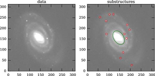
Left: postage stamp image of galaxy NGC 5364 in the r band obtained from the catalogue in Frei et al. (1996). Right: following the procedure explained in the text, we use SExtractor to detect substructures in the disc component of the galaxy (red circles), excluding most of the bulge region in the centre (green ellipse).
Once we have a catalogue of candidate structures (from a total of 350), we calculate their physical size in parsecs from their half-light radii in pixels by using the angular diameter distance to the galaxy that hosts each substructure. We assume a flat cosmology of the form specified above, and use the mean redshift to each galaxy in our subsample published by different sources as compiled by the NASA/IPAC Extragalactic Database.8
Fig. 4 shows the final flux and size distribution obtained. We fit the tail of each distribution to a power law (to avoid selection biases at the lower end of the distribution), and obtain the best-fitting exponents −2.01 ± 0.49 and −3.8 ± 0.68, respectively, and use these results as motivation to choose a power-law flux and size distributions of exponents −2 and −4 when creating substructures in each source galaxy used by SkyLens. However, these parameters can be adjusted in the code, as well as the choice of the functional form for their probability distributions.
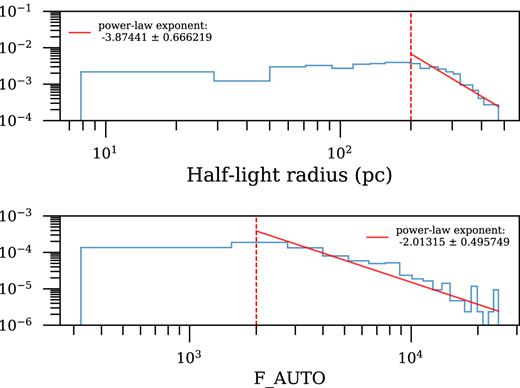
Size and luminosity distributions of substructures identified from the galaxies in Frei et al. (1996) (arbitrary amplitudes). We fit a power law to the tail of the distribution (to mitigate selection biases at the lower end of both distributions), and use the best-fitting exponents to assign a size and a luminosity to every Sérsic substructure created by skylens in each source galaxy postage stamp, as described in the text.
2.6.2 Adding substructures to the source galaxy images
For a given source galaxy image, we select a fraction Q of its total flux to be redistributed in the form of substructures. We assign a different fraction Q depending on the morphological classification of each galaxy, determined by their assigned (Coe et al. 2012) interpolated SED template (11 basis templates), ranging from N = 1 for early-type galaxies to N = 11 for starburst galaxies. Thus, we set Q to 0.05 for lenticular galaxies, Q to a random number drawn from a uniform distribution in the interval [0.2,0.4], and 0 otherwise (i.e. late-type galaxies should exhibit more regions of star formation, while no substructures are created for early-type galaxies). As with other parameters, Q can be adjusted in skylens if desired.
Each substructure is placed at a pixel location derived by creating a histogram of the surface brightness of postage stamp by means of an inverse transform sampling algorithm. In this way, the substructures will be placed mainly in locations that are proportional to the surface brightness distribution of the source galaxy. Fig. 5 shows an example of a source galaxy with and without substructures. Once the location of a particular substructure has been chosen, we model it as a Sérsic profile of index n = 3.5, with a particular size and luminosity drawn from the distributions of Fig. 4. These substructures will be subsequently created only if the image of their host galaxy in the lens plane is close enough to a critical curve such that the local magnification produced by the lens is larger than a certain threshold μt.

Galaxy from the Rafelski et al. (2015) catalogue (ID: 22245). The upper row shows the unlensed galaxy with and without knots of substructure (left- and right-hand panels). The lower row shows a similar comparison after the galaxy has been strongly lensed.
2.7 Virtual observations
As explained above, skylens has the capability of producing a virtual observation with any given instrument and/or telescope and at any desired resolution, for a particular field of view.
Finally, the images are convolved by the instrumental PSF, and different sources of noise such as sky background, Poisson, and RON are added, depending on the specified number of exposures as explained in Section 2.1.
2.8 Code validation
The different components of the skylens pipeline have been validated independently. Maturi (2017) uses simulations to corroborate the quality of the denoised source images in terms of moments of surface brightness. Vanzella et al. (2017) show in their appendix that the simulated observations created by skylens are able to produce realistic background levels.
The ray-tracing algorithm has been validated in previous versions of skylens. In addition, we use the image of local dwarf galaxy NGC 1705 [obtained by the Legacy Extragalactic UV Survey (LEGUS) survey9 in the F275W band] to further validate this part of the code. The left-hand panel of Fig. 6 shows an unlensed image of the galaxy, with the positions of a number of star clusters marked by circles. The galaxy has been placed at |$z$| = 6.14 and lensed by skylens using the lens model produced by Caminha et al. (2017) for the Frontier Field macs0416. The lensed image (PSF free) is shown in the right-hand panel of the figure, where the lensed positions of the star clusters shown in the left-hand panel – as expected by the public software lenstool10 – are marked again with circles. It can be seen that the circles enclose the lensed star clusters in the skylens simulated image. In addition, the positions of these knots also reflect the inversed parity of the image. In this particular case, we have confirmed that the position of the galaxy image in the source plane with respect to the caustics of the system is such that it is lensed into three images. The lensed image shown in the right-hand panel of Fig. 6 lies inside the resulting critical lines of the lens plane, with a negative parity.

Left: unlensed image of the galaxy NGC 1705 (LEGUS survey, F275W band). The circles mark the position of star clusters within the galaxy. Right: the source is placed at |$z$| = 6.14 and lensed with SkyLens using the lens model of the Frontiers Field macs0416 by Caminha et al. (2017). The circles mark the positions of the lensed star clusters, as expected by the software lenstool. The parity of the lensed image is negative, consistent with the position of the source with respect to the caustics and with the lensed image itself with respect to the critical lines in the lens plane.
The formalism of gravitational lensing in multiple planes described in Section 2.4 is standard and has been implemented and validated by other lensing simulation codes such as Giocoli et al. (2012), Birrer & Amara (2018), and Metcalf et al. (2018). In particular, we have verified that Birrer & Amara (2018) produce results consistent with those of skylens as shown in Fig. 2.
3 LENSING SIMULATIONS
We have simulated observations of galaxy clusters through five different telescopes and instruments to illustrate the capabilities of skylens: HST ACS WFC, WFIRST WFI, JWST NIRCam, Subaru HSC, and Euclid VIS. In the first four cases, we use the corresponding PSF-generating tools to produce sensible PSF models for different filters, and the exposure time calculators to obtain estimates of the sky background. For the latter, we refer to the Euclid Red Book (Laureijs et al. 2011) to generate a simple PSF model. We use the HXDF source catalogue and the ares lens model described in Sections 2.1 and 2.2 above.
We show the resulting images in Fig. 7 (each one with a field of view of 204 × 204 arcsec2), where we have combined three images in the ‘red’, ‘green’, and ‘blue’ channels by using the software trilogy11 (Coe et al. 2012). Fig. 8 shows a zoomed-in region of the panels in Fig. 7 illustrating a strongly lensed arc with the star-forming regions added as described in Section 2.6.2.
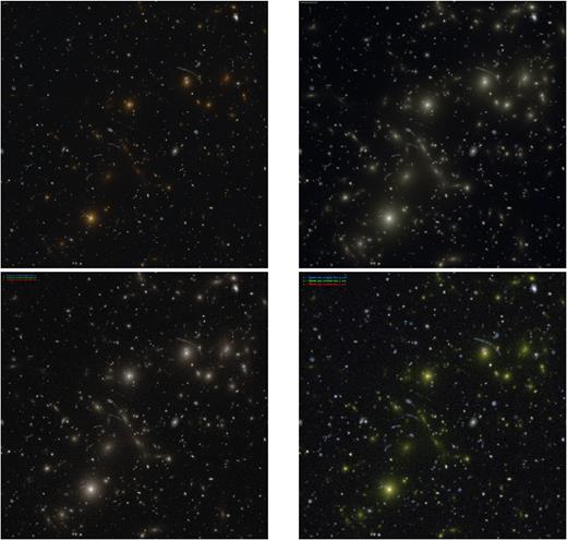
Colour composites from images produced by skylens. In all case the field of view is 204 × 204 arcsec2. Upper left: HST ACS WFC, produced by combining images in the F475W, F625W, and F775W filters. The exposure time for each image is 5000 s. Upper right: JWST NIRCam, produced by combining images in the F090W, F150W, and F200W filters. The exposure time for each image is 10 146 s. Lower left: WFIRST WFI, produced by combining images in the Y106, J129, and H158 filters. The exposure time for each image is 504 s. Lower right: Subaru HSC, produced by combining images in the g, i, and |$z$| filters. The exposure time for each image is 600 s.
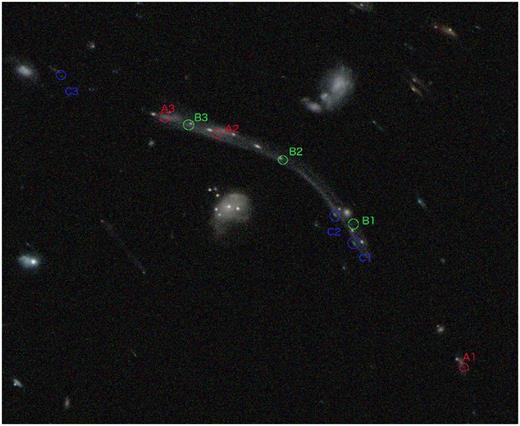
Zoomed-in of the up per central region in the HST ACS WFC image of Fig. 7. The approximate position of the multiple images from three background sources (labelled as A, B, and C) have been identified. The lensed arc is a combination of multiple lensed sources. Multiple images of knots of substructure can also be seen in the arc.
3.1 HST ACS WFC
We simulate observations through the ACS WFC of HST in the F475W, F625W, and F775Wfilters, each one with an exposure time of 5000 s. We use the web interface12 of the tiny tim software (Krist, Hook & Stoehr 2011) to generate the PSF models in each band. The PSF models have a pixel scale of 0.0495 arcsec pixel−1, but the final images will be rendered at a resolution of 0.03 arcsec pixel−1. We obtain values for the sky background (in e− pixel−1 s−1) from the measurements performed by Sokol, Anderson & Smith (2012, table 2, average backgrounds).
3.2 JWST NIRcam
We simulate observations in the imaging mode of the JWST NIRCam through the short-wavelength channel (0.6–2.3 |$\mu$|m) in the F090W, F150W, and F200W filters. We use the JWST PSF simulation tool webbpsf13 to produce PSF models in each filter. The native pixel scale of the instrument is 0.032 arcsec pixel−1, however, the NIRCam short wavelength is undersampled at 2.4 |$\mu$|m. Thus, we created PSF models sampled at a scale of 0.032/N with N = 4 to satisfy the Nyquist criterion (2p/λmF, which results in a number of dithered exposures N ≥ 3 for and f-number F of 20, a pixel pitch p of 18 |$\mu$|m and minimum wavelength λm of 0.6 |$\mu$|m). We estimate the contribution from the background in each filter from four exposures by using the JWST Exposure Time Calculator14 for NIRCam in the deep8 readout pattern with 10 groups. The values recorded for each of the three filters used are 0.318, 0.321, and 0.289 e− pixel−1 s−1, respectively. The choice of the readout pattern (deep8) and the number of exposures (N = 4) sets the exposure time of each image to 10 146 s.
3.3 WFIRST
We produce simulations in three of the four bands of the planned High Latitude Survey by the WFI of WFIRST: Y106, J129, and H158. We use the WFIRST module developed by Kannawadi et al. (2016) to obtain PSF models and sky background levels in each band.15 The near-infrared detectors of the WFI have a native pixel scale of 0.11 arcsec pixel−1; however, we draw them at a scale of |$0.11\, \text{arcsec}$|/N pixel−1 with N = 3 to avoid undersampling. The sky background model reported by galsim includes zodiacal light, stray light (10 per cent), and thermal backgrounds, and makes use of the exposure time calculator16 by Hirata et al. (2012). Including a mean dark current of 0.0015 e− pixel−1 s−1, the sky backgrounds obtained for the Y106, J129, H158, bands are 0.669, 0.654, and 0.654 e− pixel−1 s−1, respectively. The exposure time chosen for each image is 504 s (168 s exposure−1).
3.4 HSC
We use the ‘PSF Picker’ tool to generate PSF models in the g, i, and |$z$| bands of the HSC survey for the Wide Field Survey described in Aihara et al. (2018).17 The parameters used for the query are (RA, Dec.) = (180|${^{\circ}_{.}}$|0, 0|${^{\circ}_{.}}$|0), tract 9348, patch ‘8,8’, co-add, and pdr1_wide, which represent a location in the wide survey area. The pixel scale of the PSF models is 0.17 arcsec pixel−1, and the seeing values were set to 0.72, 0.56, and 0.63 arcsec in each of the g, i, and |$z$| bands, respectively, using the values in Aihara et al. (2018). We use the HSC Exposure Time Calculator18 to estimate the contributions due to the sky backgrounds. Under the conditions of grey time (7 d after new Moon), transparency of 0.9, and 60°of separation from the Moon, we obtain sky values of 35.08, 75.74, and 45.60 e− pixel−1 s−1 for the g, i, and |$z$| bands, respectively. The exposure time for each band was set to 600 s.
3.5 Euclid
Finally, we simulate an observation of Ares also with the future Euclid Space Telescope (Laureijs et al. 2011). Euclid is scheduled for launch in the early 2020s and will observe |$15\, 000$| deg2 of the sky in four bands, namely a broad riz band (VIS), and three near-infrared bands (Y, J, H). In the VIS channel the spatial resolution will be 0.1 arcsec and the observations will reach a magnitude limit of 24.5 mAB for extended sources at signal-to-noise ratio (S/N) ∼ 10, making Euclid a very promising instrument for strong lensing science.
We use the set-up of a typical Euclid observation to illustrate the multiplane functionality of skylens. For these simulations, we assume a PSF with a Moffat profile (Moffat 1969) and full width at half-maximum (FWHM) of 0.18 arcsec. We produce two images in the VIS channel. The first includes only one lens plane, as in the previous examples shown in Fig. 7. The second, includes the effects of the other two lens planes shown in the second and third upper panels of Fig. 2, in addition to that containing the mass distribution of Ares. The images are shown in Fig. 9. The effective mass distributions of the lenses in the two cases correspond to the first and to the last upper panels in Fig. 2. Clearly, the addition of other lens planes impacts on the resulting appearance of the strong lensing features. Some of the arcs are dimmed or broken into smaller arclets, while some other sources happen to be more strongly distorted. Overall, several lensed images in the right-hand panel appear shifted compared to the corresponding ones in the left-hand panel.
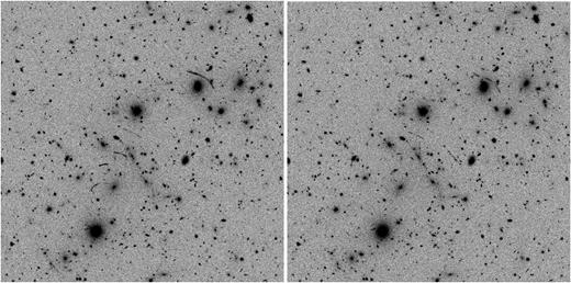
Simulated observations of Ares with Euclid in the broad riz band (VIS channel). In the left-hand panel, a single-lens plane is used, corresponding to the convergence map shown in the first panel of Fig. 2. In the right-hand panel, we stack three lens planes. The resulting effective convergence is shown in the fourth panel of Fig. 2.
4 DISCUSSION
In this section we discuss possible applications of skylens. Simulations represent a fundamental tool in gravitational lensing since there are no sources in the sky whose intrinsic shapes, before lensing, are perfectly known. Simulations with known inputs allow to calibrate lensing measurement codes and to quantify the impact of random errors (such as noise). In addition, they help to improve the understanding and characterization of systematic and modelling errors. This is useful when testing mass reconstruction codes that aim to constraint the distribution of the lens light, its mass distribution, and the background sources. In particular, the knots of substructure that represent regions of star formation included in this version of skylens will also produce multiple images in strongly lensed arcs (e.g. Fig. 8) that can place to better constraints during the source image reconstruction process. These knots of star formation are also important to better understand the images of regions of star formation in the high-redshift universe that are magnified by the effect of strong lensing.
skylens can be used to simulate gravitational arcs in the centre of galaxy clusters and to improve the modelling of strong lensing systems, crucial to exploit the information that they contain about the distribution of dark matter in galaxies and galaxy clusters. This is also important to measure the shape of dark matter haloes with precision and to detect and constrain their substructures.
The code can also be used to simulate lensing effects around galaxies, although this was not extensively discussed in this paper (Metcalf et al. 2018). Future wide galaxy surveys such as the Large Synoptic Survey Telescope (LSST; Ivezić et al. 2008) and Euclid will increase the number of strong lensing systems by up to three orders of magnitude compared to current searches (e.g. there will be about 120 000 and 170 000 galaxy–galaxy strong lenses in the cases of LSST and Euclid, respectively; Collett 2015). skylens simulations can be used to develop and train algorithms to find these systems with the efficiency and completeness required.
5 SUMMARY AND CONCLUSIONS
We have presented a new version of the ray-tracing code skylens. New additions to the code include the use of denoised source galaxies from the HXDF, which improves the resolution of the background source images as compared with previous versions of skylens. This new version of skylens is able to calculate the lensing effects due to multiple deflector planes along the line of sight, and also is able to simulate substructures in the source images that represent regions of star formation. We model these substructures as objects with a Sérsic profile, and we perform a morphological analysis of images of nearby galaxies to empirically motivate their size and luminosity distributions. skylens is able to produce observations of the images of background sources lensed by multiple deflectors along the line of sight through virtually any instrument and telescope – both ground- and space-based. The mass distribution of the lenses (produced either analytically or numerically) is used to generate a deflection angle field per lens plane. Multiple lens planes can be used to include lensing effects by any mass along the line of sight. Once the total throughput of the system, a model for the PSF, and the characteristics of the instrument and telescope are specified, skylens will produce a simulated image of an observation (including noise) for a given field of view and exposure time.
As an example of the simulations that can be generated with skylens we have created images in multiple filters for several imaging instruments of current and future space- and ground-based observatories: HST ACS WFC, WFIRST WFI, JWST NIRcam, Subaru’s HSC, and Euclid’s VIS. Simulations with known input allow for the testing, calibration, and improvement of lens modelling algorithms, in addition to providing a means to tests for the impact of different sources of random and systematic errors. The regions of star formation included in the source images of this version of skylens will allow, for example, to provide better constraints on source image reconstructions and lens models. The simulations created by skylens can also be utilized to train algorithms that automatize the search for strong lensing systems in large data sets.
We will make skylens available through the Bologna Lens Factory portal.19
ACKNOWLEDGEMENTS
We acknowledge support from the Italian Ministry of Foreign Affairs and International Cooperation (MAECI), Directorate General for Country Promotion, from ASI via contract ASI/INAF/I/023/12/0. We acknowledge support from grant HST-AR-13915.004-A of the Space Telescope Science Institute. AAP is supported by the Jet Propulsion Laboratory. JR is being supported in part by the Jet Propulsion Laboratory. The research was carried out in part at the Jet Propulsion Laboratory, California Institute of Technology, under a contract with the National Aeronautics and Space Administration. MMa was supported by the SFB-Transregio TR33 ‘The Dark Universe’. ©2017. All rights reserved.
Footnotes
The catalogue can be found at https://asd.gsfc.nasa.gov/UVUDF/catalogs.html
The Sérsic index of the knots of structure formation is a parameter that can be adjusted in the code.
Such as detect_minarea, detect_maxarea, and detect_thresh.
https://archive.stsci.edu/prepds/legus/dataproducts-public.html
https://jwst.stsci.edu/science-planning/proposal-planning-toolbox/psf-simulation-tool-webbpsf
We use galsim v1.4. The WFIRST module is called galsim.wfirst, and the PSF and sky backgrounds are obtained by calling the utilities galsim.wfirst.getbandpasses() and galsim.wfirst.getskylevel(), respectively.
The tool can be found at https://hsc-release.mtk.nao.ac.jp/psf/pdr1/
