


ABSTRACT
We define and characterize a sample of 1.3 million galaxies extracted from the first year of Dark Energy Survey data, optimized to measure baryon acoustic oscillations (BAO) in the presence of significant redshift uncertainties. The sample is dominated by luminous red galaxies located at redshifts |$z$| ≳ 0.6. We define the exact selection using colour and magnitude cuts that balance the need of high number densities and small photometric redshift uncertainties, using the corresponding forecasted BAO distance error as a figure-of-merit in the process. The typical photo |$z$| uncertainty varies from |$2.3{{\ \rm per\, cent}}$| to |$3.6{{\ \rm per\, cent}}$| (in units of 1+|$z$|) from |$z$| = 0.6 to 1, with number densities from 200 to 130 galaxies per deg2 in tomographic bins of width Δ|$z$| = 0.1. Next, we summarize the validation of the photometric redshift estimation. We characterize and mitigate observational systematics including stellar contamination and show that the clustering on large scales is robust in front of those contaminants. We show that the clustering signal in the autocorrelations and cross-correlations is generally consistent with theoretical models, which serve as an additional test of the redshift distributions.
1 INTRODUCTION
The use of the imprint of baryon acoustic oscillations (BAO) in the spatial distribution of galaxies as a standard ruler has become one of the common methods in current observational cosmology to understand the Universe. The physics that causes BAO is well understood. Primordial perturbations generated acoustic waves in the photon–baryon fluid until decoupling (|$z$| ∼ 1100). These sound waves lead to the large oscillations observed in the power spectrum of the cosmic microwave background (CMB) anisotropies, but they are also visible in the clustering of matter, and therefore galaxies, as a high-density region around the original source of the perturbation, at a distance given by the sound horizon length at recombination. This high-density region shows as a small excess in the number of pairs of galaxies separated by ∼150 Mpc. Since the sound horizon is very precisely measured in the CMB (Planck Collaboration XIII 2016), the BAO measurements can be used as a standard ruler. This is therefore a geometrical probe of the expansion rate of the Universe that maps the angular diameter distance and the Hubble parameter as functions of the redshift. There have now been multiple detections of the BAO in redshift surveys (Percival et al. 2001; Cole et al. 2005; Eisenstein et al. 2005; Percival et al. 2010; Beutler et al. 2011; Blake et al. 2011; Delubac et al. 2015; Ross et al. 2015; Alam et al. 2017; Bautista et al. 2017; Ata et al. 2018), and it is considered as one of the main cosmological probes for current and planned cosmological projects.
A key feature of the BAO method is the fact that the sound horizon length is large, and therefore very deep and wide galaxy surveys are needed in order to reach precise measurements of the BAO scale. But, at the same time, this large scale protects the BAO feature from large corrections due to astrophysical and non-linear effects of structure formation and therefore from systematic errors, making BAO a solid probe of the expansion rate of the Universe.
The Dark Energy Survey (DES) is one of the most important of the currently ongoing large galaxy surveys, and, as its name suggests, it is specially designed to attack the problem of the physical nature of the dark energy. It will do it using several independent and complementary methods at the same time. One of them is the precise study of the spatial distribution of galaxies, and in particular, the BAO standard ruler. DES is a photometric survey, which means that its precision in the measurement of redshifts is limited, preventing the measurement of the Hubble parameter evolution. However, the evolution of the angular distance with redshift is possible through the measurement of angular correlation functions (Seo & Eisenstein 2003; Blake & Bridle 2005; Padmanabhan et al. 2005; Padmanabhan et al. 2007; Crocce et al. 2011; Sánchez et al. 2011; Carnero et al. 2012; Seo et al. 2012; de Simoni et al. 2013)
Although DES will only measure BAO in the angular distribution of galaxies, a determination of the photometric redshift as precise as possible brings several benefits. It allows a finer tomography in the mapping of the BAO evolution with the redshift and makes the analysis cleaner, reducing the correlations between redshift bins. A sample of luminous red galaxies (LRGs) would fit these requirements (Padmanabhan et al. 2005, 2007). LRGs are luminous and massive galaxies with a nearly uniform spectral energy distribution but with a strong break at 4000 Å in the rest frame. These features allow a clean selection and an accurate determination of the redshift for these type of galaxies, even in photometric surveys. This selection has been done previously for imaging data at |$z$| ≲ 0.6 (Padmanabhan et al. 2005). But the BAO scale has already been measured with high precision in this redshift range (e.g. Alam et al. 2017 and references therein). In order to go to higher redshifts, the selection criteria need to be redefined. The 4000 Å feature enters the i band at |$z$| = 0.75, and the methods used in previous selections are not valid anymore.
In this paper, we describe the selection of a sample of red galaxies to measure BAO in DES, which includes, but is not limited to, LRGs. The selection is defined by two conditions. On the one hand, keep the determination of the photometric redshift as precise as possible. On the other hand, keep the galaxy density high enough to have a BAO measurement that is not limited by shot noise.
In order to guide our efforts to select an optimized sample for measuring BAO distance scales, we rely on Fisher matrix forecasts. Seo & Eisenstein (2007) provide a framework and simple formulae to predict the precision that one can achieve with a given set of galaxy data. Thus, we will test how Fisher matrix forecasts vary given the variations obtained for the number density and estimated redshift uncertainty given a set of colour-magnitude cuts.
This paper, detailing the BAO sample selection, is one of a series describing the supporting work leading to the BAO measurement using DES Y1 data presented in The DES Collaboration (2017; hereafter DES-BAO-MAIN). As part of such series, one paper presents the mock galaxy catalogues, Avila et al. (2018; hereafter DES-BAO-MOCKS). Gaztañaga et al. (in preparation) discuss in detail the photo |$z$| validation, and we denote it DES-BAO-PHOTOZ. Chan et al. (2018), from now on DES-BAO-θ-METHOD, introduce the BAO extraction pipeline using a tomographic analysis of angular correlation functions, while Camacho et al. (2018) present the study of the angular power spectrum (hereafter DES-BAO-ℓ-METHOD). Lastly, Ross et al. (2017a), in what follows referred to as DES-BAO-s⊥-METHOD, introduced a novel technique to infer BAO distances using the 3D correlation function binned in projected separations.
This paper is organized as follows: In Section 2, a description of the main features of the DES-Y1 catalogue is given; in Section 3, we give a detailed description of the selection cuts that define the data sample that has been used to measure the BAO scale in DES; section 4 contains a description of the procedure that has been developed and applied in DES in order to ensure the quality of the photometric redshift determination and to determine its relation with the true redshift; Section 5 describes the masking scheme and the treatment of the variable depth in the survey; Section 6 is a description of the analysis and mitigation of observational systematic errors on the clustering measurement; and finally, Section 7 describes the measured two-point correlation and cross-correlation functions and their evolution with redshift for the selected sample. We finish with our conclusions in Section 8.
2 DES Y1 DATA
The BAO galaxy sample we will define in this work uses the first year of data (Y1) from the DES. This photometric data set has been produced using the Dark Energy Camera (DECam, Flaugher et al. 2015) observations, processed and calibrated by the DES Data Management system (DESDM; Sevilla et al. 2011; Mohr et al. 2012; Morganson et al. 2018) and finally curated, optimized, and complemented into the Gold catalog (hereafter denoted ‘Y1GOLD’), as described in Drlica-Wagner et al. (2017). For each band, single exposures are combined in coadds to achieve a higher depth. We keep track of the complex geometry that the combinations of these dithered exposures will create at each point in the sky in terms of observing conditions and survey properties (SPs). Objects are detected in chi-squared combinations of the r, i, and |$z$| coadds to create the final coadd catalog (Szalay, Connolly & Szokoly 1999).
Y1GOLD covers a total footprint of more than 1800 deg2; this footprint is defined by a healpix (Górski et al. 2005) map at resolution Nside = 4096 and includes only area with a minimum total exposure time of at least 90 s in each of the griz bands, and a valid calibration solution (see Drlica-Wagner et al. 2017 for details). This footprint is divided into several disjoint sub-regions that encompass the supernova survey areas, a region overlapping stripe 82 from the SDSS footprint (S82; Annis et al. 2014) and a larger area overlapping with the South Pole Telescope coverage (SPT; Carlstrom et al. 2011). Fig. 1 shows the angular distribution of galaxies, selected as described in Section 3, that includes these two areas. A series of veto masks, including masks for bright stars and the Large Magellanic Cloud among others, reduce the area by ∼500 deg2, leaving 1336 deg2 suitable for LSS study. Other areas that are severely affected by imaging artefacts or otherwise have a high density of image artefacts are masked out as well. Section 5 provides a full account of the final mask used in combination with the final BAO sample. ‘Bad’ regions information is propagated to the ‘object’ level using the flags_badregion column in the catalogue. Finally, individual objects that have been identified as being problematic by the DESDM processing or by the vetting process carried out by the scientists in the collaboration are flagged when configuring the catalogue (this is done through the flags_gold column). All data we describe in this and in subsequent sections are drawn from quantities and maps released as part of the DES Y1 Gold catalog and are fully described in Drlica-Wagner et al. (2017).
![Angular distribution and projected density of the DES-Y1 red galaxy sample described in this paper and subsequently used for BAO measurements. The unmasked footprint comprises the two largest compact regions of the data set: one in the Southern hemisphere of 1203 deg2, overlapping SPT observations (Carlstrom et al. 2011), and 115 deg2 near the celestial equator, overlapping with S82 (Annis et al. 2014). The sample consists of about 1.3 million galaxies with photometric redshifts in the range [0.6−1.0] and constitutes the baseline for our DES-Y1 BAO analysis.](https://oup.silverchair-cdn.com/oup/backfile/Content_public/Journal/mnras/482/2/10.1093_mnras_sty2522/1/m_sty2522fig1.jpeg?Expires=1749862295&Signature=J1rnEi2N04B0hUVynk6txWzqlWptkA8CuEI6RF7J~wTeKK4OOF6NtLm4MRXHSCuztMCUBfbc6loyJftADbAsj-FgZbPc3mYQ6sNKdIqRGIZcgODuE8vFLS6ixDrErIHgAFx0GrTDYXWH3-h7gPqkj4Y3PcMMGJAH2go1YE9Z09awjnal-vRpV0GvMzce5wLZAHYWGpe6A34UMuG51korvGQbE8axlHBnC0RE3RXXsD66KdaVdm53ulZv92Ct~yexfkOaIO7xyQ0iMo6s6ejYnhsIxQjEFqNvjNs7bXUwaiZuC~JYeGvv4MERLvwcytes3lKlGGJcyqNeZvrr1CgJfw__&Key-Pair-Id=APKAIE5G5CRDK6RD3PGA)
Angular distribution and projected density of the DES-Y1 red galaxy sample described in this paper and subsequently used for BAO measurements. The unmasked footprint comprises the two largest compact regions of the data set: one in the Southern hemisphere of 1203 deg2, overlapping SPT observations (Carlstrom et al. 2011), and 115 deg2 near the celestial equator, overlapping with S82 (Annis et al. 2014). The sample consists of about 1.3 million galaxies with photometric redshifts in the range [0.6−1.0] and constitutes the baseline for our DES-Y1 BAO analysis.
The photometry used in this work comes mainly from two different sources:
the SExtractor (Bertin & Arnouts 1996) AUTO magnitudes, which are derived from the best-matched elliptical aperture according to the coadd object elongation and angle in the sky, measured using the coadded object flux;
Multi-Object Fitting (MOF) pipeline, which performs a multi-epoch and multiband fit of the shape and per-band fluxes directly on the single epoch exposures for each of the coadd objects, with additional neighbouring light subtraction. This is described in more detail in Drlica-Wagner et al. (2017).
Using these photometric measurements, we will consider three different photometric redshift catalogues. Two of them are built using Bayesian photometric redshift (BPZ; Benítez 2000), a Bayesian template-fitting method, and another using a machine learning approach: the Directional neighbourhood Fitting (DNF) algorithm as described in De Vicente, Sánchez & Sevilla-Noarbe (2016). They are combined with the photometric quantities described above and used as follows:
BPZ run with AUTO magnitudes (hereafter |$z$|BPZ–AUTO) used for making the selection of the overall sample.
BPZ run with MOF magnitudes (hereafter |$z$|BPZ–MOF) used for redshift binning and transverse distance calculation, finally used as secondary catalogue to show the robustness of the analysis.
DNF run with MOF magnitudes (hereafter |$z$|DNF–MOF) used for redshift binning and transverse distance calculation, finally used as our fiducial catalogue.
We should note that BPZ with AUTO magnitudes is part of the DESDM data reduction pipeline and is available early on in the catalogue making. This explains why we used that particular combination for sample selection. We did not find, and do not expect, the relative optimization of the sample selection and cuts to depend much on the particular photo |$z$| catalogue (but the final absolute error on BAO distance measurement does).
In Section 4, we summarize the validation performed to select and characterize the true redshift distributions of the binned samples, which is described in detail in DES-BAO-PHOTOZ.
Throughout our analysis, we assume the redshift estimate of each galaxy to be the mean redshift of the redshift posterior for BPZ, or the predicted value for the object in the fitted hyper-plane from the DNF code (see De Vicente et al. 2016). Any potential biases from these estimates are calibrated as described in Section 4.
3 SAMPLE SELECTION
In this section, we describe the steps towards the construction of a red galaxy dominated sample, optimized for BAO measurements, starting from the data set described in Section 2. The selection is performed over the largest continuous regions of the survey at this point, namely SPT and S82. Objects are selected so that we avoid imaging artefacts and pernicious regions with foreground objects using the cuts on flags_badregion and flags_gold described therein. In the rest of this section, we go into finer details on the flux, colour, and star-galaxy separation selection.
In Table 1, we summarize this sample selection, including references to the sections where these cuts are explained.
Complete description of the selection performed to obtain a sample dominated by red galaxies with a good compromise of photo |$z$| accuracy and number density, optimal for the BAO measurement presented in DES-BAO-MAIN. The redshifts of the resulting catalogue are then computed using different codes (BPZ and DNF) as described in Section 2. Therefore, any subsequent photo |$z$| selection can be done either with |$z$|photo from BPZ or DNF.
| Keyword | Cut | Description |
|---|---|---|
| Gold | Observations present in the Gold catalog | Drlica-Wagner et al. (2017) |
| Quality | flags_badregion < 4; flags_gold = 0 | Section 5; Section 2 |
| Footprint | 1336 deg2 (1221 deg2 in SPT and 115 deg2 in S82) | Fig. 1 Section 5 |
| Colour Outliers | −1 < gauto−rauto < 3 | Section 3.1 |
| −1 < rauto−iauto < 2.5 | Section 3.1 | |
| −1 < iauto−|$z$|auto < 2 | Section 3.1 | |
| [Optimized] Colour Selection | (iauto−|$z$|auto) + 2.0(rauto−iauto) > 1.7 | Section 3.4.1 |
| [Optimized] Completeness Cut | iauto < 22 | Section 3.1 |
| [Optimized] Flux Selection | 17.5 < iauto < 19.0 + 3.0|$z$|BPZ–AUTO | Section 3.4.2 |
| Star–galaxy separation | spread_model_i + (5/3) spreaderr_model_i >0.007 | Section 3.2 |
| Photo |$z$| range | [0.6−1.0] | Section 4 |
3.1 Completeness and colour outliers cuts
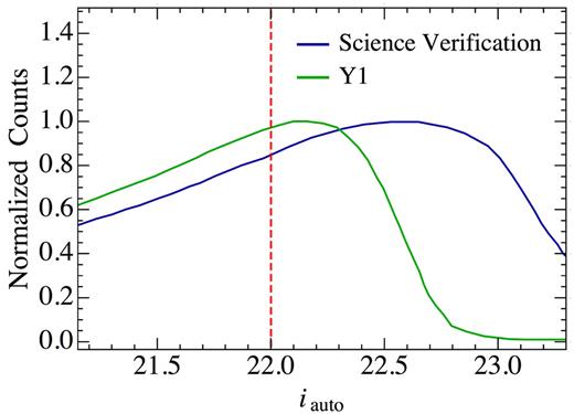
Measurement of the trade-off between area and number of objects as a function of magnitude limit and sample flux limit in Y1GOLD and SV. For a given iauto-band ‘threshold’ value, we select all regions that have a deeper limiting magnitude that this value (10σ depth limit > ‘threshold’) and count the galaxies brighter than the ‘threshold’ value over those regions. These should be complete samples at each threshold value. Number counts are shown normalized to their maximum in the figure.
Colour outliers that are either unphysical or from special samples (Solar system objects, high redshift quasars) are removed as well, to avoid extraneous photo |$z$| populations in the sample (see Table 1).
3.2 Star–galaxy separation
Removing stars from the galaxy sample is an essential step to avoid the dampening of the BAO signal-to-noise (Carnero et al. 2012) or the introduction of spurious power on large scales (Ross et al. 2011a). Stellar contamination affects the broad shape of the measurement, and so we want to minimize it to be able to fit the BAO template properly. However, it does not appreciably affect the location of the BAO feature, so we do not need to push for 100 per cent purity. Any residual contamination is then taken care of using the weighting scheme detailed in Section 6.
In Fig. 3, we show the estimated star sample contamination for different thresholds of this cut, using the relation between galaxy density and a map of stellar density built from Y1GOLD (a methodology that is described in detail in Section 6). The error bars displayed are the fitting errors obtained for the intercept when parametrizing the contamination level using a linear relationship between the galaxy density as a function of stellar density. Note that a threshold of 0.007 reduces the contamination level to less than |$5{{\ \rm per\, cent}}$| across the redshift range of interest. In Table 2, we report a consistent or smaller level of stellar contamination, using a similar estimation, in the catalogues with MOF photometry, both for BPZ and DNF (see Section 6). In Fig. 4, we also include in the middle figure the track from the stellar locus, which showcases the reason why the first two redshift bins are more affected by stellar contamination, as it crosses the elliptical templates at these redshifts. To further illustrate this, in Fig. 5 we show the distribution of the mean photometric redshifts for stars (selected using the criterion |$|{\tt \mathbf wavg\_spread\_model\_i}| \lt 0.002$|, a more accurate variant of |${\tt \mathbf spread\_model\_i}$| using single-epoch, suitable for moderate to bright magnitude ranges) showcasing how they will contaminate preferentially the second redshift bin, following the same trend as shown in Table 2.
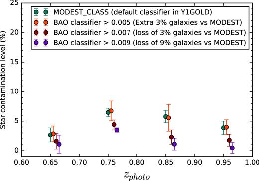
Contamination of galaxy sample from stars as a function of redshift and star–galaxy separation threshold, as measured using galaxy density versus stellar density plots (from a pure stellar sample). The MODEST classifier is defined in Drlica-Wagner et al. (2017) as the default star galaxy classifier (based on |${\tt \mathbf spread\_model}$| and |${\tt \mathbf wavg\_spread\_model}$|). ‘BAO classifier’ stands for a cut in |${\tt \mathbf spread\_model\_i} + (5.0/3.0){\tt \mathbf spreaderr\_model\_i}$|. A threshold of 0.007 provides an important decrease of contamination with a minor adjustment in the number of galaxies, which becomes significantly more severe at higher thresholds for a very similar purity. The redshift binning here uses |$z$|BPZ–AUTO.
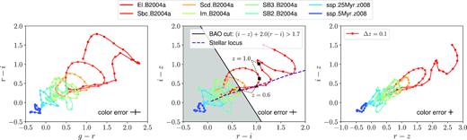
Evolution of BPZ templates in colour–colour space. Each dot corresponds to a different redshift in steps of 0.1, ranging from |$z$| = 0.0 to |$z$| = 2.0. The shadowed region in the central panel is excluded from the sample. The black dots indicate the position of |$z$| = 0.6 (triangles), and |$z$| = 1.0 (squares) for the two reddest templates. Also shown, for reference, is the stellar locus as a purple dashed line. The inset crosses indicate an estimate of the error in the colours, arising from photometric errors, from a sub-sample of DES Y1 galaxies selected in the range 21 < iauto < 22 (see text for more details).

Characteristics of the DES-Y1 BAO sample, as a function of redshift. Results are shown for a selection of the sample in bins according to DNF photo |$z$| (|$z$|photo) estimate in top of the table and BPZ in the bottom, both with MOF photometry. Here, |$\bar{z}=\lt z_{\mathrm{ true}}\gt$| is the mean true redshift, σ68 and W68 are the 68 per cent confidence widths of (|$z$|photo−|$z$|true)/(1 + |$z$|true) and |$z$|true, respectively, all estimated from COSMOS–DES validation with SVC correction, as detailed in Section 4 and Fig. 7. fstar is the estimated stellar contamination fraction, see Section 6.
| DNF | Ngal | bias | |$\bar{z}$| | σ68 | W68 | fstar |
| 0.6−0.7 | 386 057 | 1.81 ± 0.05 | 0.652 | 0.023 | 0.047 | 0.004 |
| 0.7−0.8 | 353 789 | 1.77 ± 0.05 | 0.739 | 0.028 | 0.068 | 0.037 |
| 0.8−0.9 | 330 959 | 1.78 ± 0.05 | 0.844 | 0.029 | 0.060 | 0.012 |
| 0.9−1.0 | 229 395 | 2.05 ± 0.06 | 0.936 | 0.036 | 0.067 | 0.015 |
| BPZ | Ngal | bias | |$\bar{z}$| | σ68 | W68 | fstar |
| 0.6−0.7 | 332 242 | 1.90 ± 0.05 | 0.656 | 0.027 | 0.049 | 0.018 |
| 0.7−0.8 | 429 366 | 1.79 ± 0.05 | 0.746 | 0.031 | 0.076 | 0.042 |
| 0.8−0.9 | 380 059 | 1.81 ± 0.06 | 0.866 | 0.034 | 0.060 | 0.015 |
| 0.9−1.0 | 180 560 | 2.05 ± 0.07 | 0.948 | 0.039 | 0.068 | 0.006 |
3.3 Selecting red luminous galaxies
The next step is to select from Y1GOLD a sample dominated by LRGs as their typical photo |$z$| estimates are more accurate than for the average galaxy population because of the 4000 Å Balmer break in their spectra. This feature makes redshift determination easier even with broad-band photometry (Padmanabhan et al. 2005). In addition, we want our BAO sample to cover redshifts larger than 0.6 as there are already very precise BAO measurements for |$z$| < 0.6 (see e.g. Cuesta et al. 2016; Beutler et al. 2017; Ross et al. 2017b).
We have tested that, while a very stringent selection can be done to yield minimal photo |$z$| errors, e.g. with the redMaGiC algorithm (Rozo et al. 2016), it does not lead to optimal BAO constraints because the sample ends up being very sparse, with ∼200 000 galaxies in Y1GOLD at |$z$| > 0.6 (Elvin-Poole et al. 2018). Instead, we will follow an alternative path and apply a standard selection in colour–colour space to isolate red galaxies at high redshift, balancing photo |$z$| accuracy and number density with a BAO figure-of-merit in mind.
In Fig. 4, we show the evolution in redshift of the eight spectral templates used in BPZ, which includes one typical red elliptical galaxy, two spirals, and five blue irregulars/starbursts (colour coded) based on Coleman, Wu & Weedman (1980) and Kinney et al. (1996). We compute the expected observed DES broad-band magnitudes for these templates as a function of redshift and show them in different colour–colour combinations. The tracks are evolved from |$z$| = 0 to |$z$| = 2.0 in steps of 0.1 (marked with dots). We will use them to define cuts in colour–colour space intended to isolate the red templates.
In real data, galaxy colours have an uncertainty due to photometric errors, which effectively thicken those tracks. In order to provide an estimate for this, we computed the errors in the colours for a sub-sample of Y1GOLD galaxies with 21 < iauto < 22 (the typical range of magnitudes that we explore next to define the BAO sample). For each galaxy, we estimate the colour error adding in quadrature the corresponding magnitude errors.1 The average error in each corresponding colour is shown with a cross at the bottom right inset label of the three panels of Fig. 4. Their values are 0.128, 0.073, 0.067, and 0.076 for (g–r, r–i, i–z,andr–z), respectively.
In addition, a model of a red elliptical galaxy spectrum is shown in Fig. 6, redshifted to |$z=0.4,\, 0.8,\, 1.15$|, where the notable 4000 Å break crosses from g → r, r → i, and i → |$z$|. This suggests that for |$z$| > 0.6 the strongest evolution in colour will be for i−|$z$| and r−i, and hence we will focus in these colour combinations in what follows (that moreover has the smallest error).
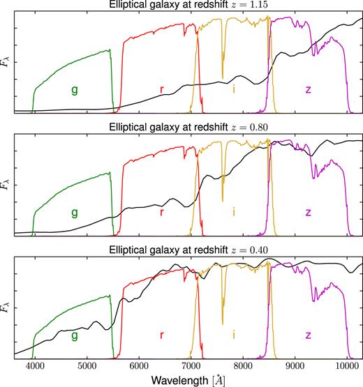
Elliptical model spectrum used in template-based fitting code BPZ. Overplotted are the DES response filters g,r,i,z. The template has been redshifted to |$z=0.4,\, 0.8,\, 1.15$|, where the notable 4000 Å break crosses from g → r, r → i, and i → |$z$|.
Note how the transition of the 4000 Å break from one band to another abruptly bends the colour–colour tracks in Fig. 4. However, this applies mainly to elliptical templates, and recent star formation will dampen this effect.
3.4 Optimization of the colour and magnitude cuts for BAO
Optimizing the actual sample selection for the measurement of BAO in imaging data is considerably different than doing so for spectroscopic data. In the latter case, one basically needs to maximize the area (or volume) provided that |${\bar{n}} P \gt 1$| (where |${\bar{n}}$| is the galaxy density and P the power spectrum). For imaging data, the photometric redshift accuracy plays a vital role. Worse photo |$z$| error degrades the signal as the galaxy radial separations are smeared out (this also complicates the definition of survey volume). In turn, the best photo |$z$|’s are typically obtained for very bright, and low-density samples. Therefore, there is a non-trivial interplay to maximise BAO signal to noise.
In DES-BAO-s⊥-METHOD, we discussed in detail how to fold in the photo accuracy into an effective2. However, computing |${\bar{n}}_{\rm eff}$| is cumbersome and as complicated as doing an actual BAO forecasting. Therefore, we decided to follow this latter path and rely on the Fisher matrix forecast formalism described in Seo & Eisenstein (2007). Provided with a concrete set of colour-magnitude cuts, we measure in the data the number density and redshift uncertainty in several tomographic bins within 0.6 ≤ photo |$z$| ≤ 1.0 and assume a clustering amplitude. We then use the formulae from Seo & Eisenstein (2007) to predict the precision that one can achieve with that set of galaxy data properties. We repeat this process for a different set of cuts until an optimal BAO distance error is achieved.
Through this process we fix the clustering amplitude, assuming a galaxy bias of b = 1.6 for all calculations. This is the bias found in Crocce et al. (2016) for a flux-limited sample (i < 22.5) at redshifts |$z$| ∼ 0.9, selected from DES science verification (SV) data. Since that redshift and magnitude are compatible with what we expect in this paper, we consider b = 1.6 a representative value. More precise measurements are expected for more biased samples, but the galaxy bias for any given sample is not known a priori and the redshift uncertainty and number density are the more dominant factors.
For illustrative purposes, we show in Table 3 the variation in BAO distance error achieved by changing the number density and photo |$z$| accuracy away from those at the optimal cuts described next. We also include the variation with survey area. As pointed before, BAO distance errors are very sensitive to photo |$z$| accuracy.
Sensitivity of the forecasted BAO distance error to variations in density, photometric redshift errors, and survey area. Note that these variations are considered individually, neglecting their correlations. Baseline values are those corresponding to the optimal cuts discussed in Section 3.4.
| |${\rm Property\, variation}$| | |${\rm Forecasted\, BAO\, distance\, error}$| |
|---|---|
| 10% worse photo-|$z$| | 8% worse |
| 20% worse photo-|$z$| | 16 % worse |
| 10% lower density | 3% worse |
| 20% lower density | 6 % worse |
| 10% smaller area | 2.8% worse |
| |${\rm Property\, variation}$| | |${\rm Forecasted\, BAO\, distance\, error}$| |
|---|---|
| 10% worse photo-|$z$| | 8% worse |
| 20% worse photo-|$z$| | 16 % worse |
| 10% lower density | 3% worse |
| 20% lower density | 6 % worse |
| 10% smaller area | 2.8% worse |
3.4.1 Optimization of the colour cut
The cut was chosen in this form following the discussion in Section 3.3 (see Fig. 4), as it allows us to select more likely the reddest galaxies that are the ones with lower uncertainties in their photometric redshift determination and still present a high enough number density.
Samples were produced across a grid of a1 and a2 values, calculating the number of galaxies Ngal and a mean width of the photo |$z$| distribution σ|$z$|/(1 + |$z$|) for each sample, after splitting the galaxy in tomographic bins. For BPZ, we estimated σ|$z$| averaging in each tomographic bin the width of the individual redshift posterior distributions function (PDF) provided per galaxy.
The BAO forecast using the algorithm of Seo & Eisenstein (2007) is then run for the Ngal and σ|$z$|/(1 + |$z$|) of each sample and final values of a1 and a2 are selected to minimize the forecasted BAO uncertainty, finding a balance between galaxy number density and redshift uncertainty. In order to give a sense for the sensitivity of such process, we note there is a slight degeneracy when increasing a1 and a2 simultaneously, resulting in similar forecasted BAO uncertainties. However, deviations from this degeneracy direction lead to significant degradation in the forecasted error. For example, doubling a1 leads to a degradation of the forecasted error by approximately 0.01 (from |$5{{\ \rm per\ cent}}$| to |$6{{\ \rm per\ cent}}$| roughly). The values used in this analysis are a1 = 2.0 and a2 = 1.7. Fig. 4 shows the colour cut in the central panel, where the shadowed region is excluded from the sample.
3.4.2 Optimization of the magnitude cut
The final forecasted uncertainty on angular diameter distance combining all the tomographic bins is |${\sim } 4.7{{\ \rm per\ cent}}$|. Note that the discussion in this section only has as a goal the definition of the sample. The real data analysis with the sample defined here, and the final BAO error achieved, will of course depend on many other variables that were not considered up to this point. Such as the quality of photometric redshift errors, analysis, and mitigation of systematics, use of the full covariance and optimized BAO extraction methods.
None the less, we stress that the forecasted error obtained in this section matches the one from the analysis of mock simulations, see e.g. DES-BAO-θ-METHOD, and is in fact quite close to the final BAO error obtained in DES-BAO-MAIN. In the following sections, we discuss the various components that will enter the real data analysis, starting with the validation of photometric redsfhit errors and the estimate of redshift distributions.
4 PHOTOMETRIC REDSHIFTS
The photometric redshifts used for redshift binning and transverse distance computations in our fiducial analyses are derived using the DNF algorithm (De Vicente et al. 2016), which is trained with public spectroscopic samples as detailed in Hoyle et al. (2017). For comparison, we also discuss next the BPZ (Benítez 2000) that we find slightly less performant in terms of the error with respect to ‘true’ redshift values (see next). In both cases, we use MOF photometry that provides |${\sim } 10\text{--}20{{\ \rm per\, cent}}$| more accurate photo |$z$| estimates with respect to the equivalent estimates using SExtractor MAG_AUTO quantities from coadd photometry. In this section, we summarize the steps taken to arrive at these choices, based on a validation against data over the COSMOS field.
We recall that throughout this work we use the individual object’s mean photo |$z$| from BPZ (not to be confused with the mean value |$\bar{z}=\lt z\gt$| of the sample) and the predicted value in the fitted hyper-plane from the DNF code, as our point estimate for galaxy redshifts. As for the estimates of the N(|$z$|) from the photo |$z$| codes, for comparison with our fiducial choice based on the COSMOS narrow band p(|$z$|), we will use the stacking of Monte Carlo realizations of the posterior redshift distributions p(|$z$|) for the BPZ estimates, or the stacking from the nearest neighbour redshifts from the training sample, in the case of DNF (henceforth we’ll call these stack N(|$z$|)). Fig. 7 shows the stack N(|$z$|) (yellow histograms) in all four redshift bins for our fiducial DNF photo |$z$| analysis.
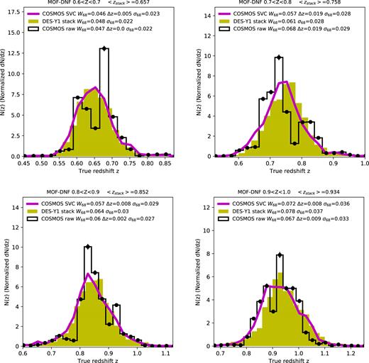
Normalized redshift distributions for our different tomographic bins of DNF–MOF photo |$z$|. Stack N(|$z$|) is shown for the full DES-Y1 BAO sample (yellow histograms). The black histogram (with Poisson error bars) shows the raw 30-band photo |$z$| from the COSMOS–DES validation sample. The magenta lines show the same sample corrected by sample variance cancellation (SVC, see text), which is our fiducial estimate. The labels show the values of W68, σ68, and Δ|$z$| = < |$z$|stack > − < |$z$| > and in each case, see also Table 2.
4.1 COSMOS validation
As detailed in DES-BAO-PHOTOZ, we check the performance of each code using redshifts in the COSMOS field (which are not part of the training set in the case of DNF), following the procedure outlined in Hoyle et al. (2017). These redshifts are either spectroscopic or accurate (σ68 < 0.01) 30-band photo |$z$| estimates from Laigle et al. (2016). Both validation samples give consistent results in our case because the samples under study are relatively bright.
The COSMOS field is not part of the DES survey. However, a few select exposures were done by DECam that were processed by DESDM using the main survey pipeline. We call this sample DES–COSMOS. Because the COSMOS area is small (2 deg2) and DECam COSMOS images were deeper and not taken as part of the main DES-Y1 Survey, we need to first resample the DES–COSMOS photometry to make it representative of the full DES Y1 samples that we select in our BAO analysis. Hence, we add noise to the fluxes in the DES–COSMOS catalog to match the noise properties of the fluxes in the DES-Y1 BAO sample, this is what we refer to as resampled photometry. Then for each galaxy in the DES-Y1 BAO sample, we select the galaxy in DES–COSMOS whose resampled flux returns a minimum χ2 when compared to the DES-Y1 BAO flux (the χ2 combines all bands, g, r, i, and |$z$|). This is done for every galaxy in the DES-Y1 BAO sample to make up the ‘COSMOS-Validation’ catalog, which by construction has colours matching those in the DES-Y1 BAO sample. The ‘true’ redshift is retrieved from the spectroscopic/30-band photo |$z$| of this match.
We then run the DNF photo |$z$| code over the COSMOS-Validation catalog to select four redshift bin samples in the same way as we did for the full DES-Y1 BAO sample. We use the ‘true’ redshifts from the COSMOS-validation catalogs to estimate the N(|$z$|) in each redshift bin by normalizing the histogram of these true redshifts.
Results are shown as histograms in Fig. 7, which are compared to the stack N(|$z$|) from the photo |$z$| code, for reference. The black histograms show large fluctuations that are caused by real individual large-scale structures in the COSMOS field. This can be seen by visual inspection of the maps. This sampling variance comes from the relatively small size of the COSMOS validation region. There is also a shot noise component, indicated by the error bars over the black dots, but it is smaller. In the next section, we briefly describe the methodology to correct for this to be able to use this validation sample effectively.
4.2 Sample variance correction
As detailed in DES-BAO-PHOTOZ, we apply a sample variance correction (SVC) to the data and test this method with the Halogen mocks described in DES-BAO-MOCKS. In what follows, we provide a summary of such process and its main results.
We use the VIPERS catalog (Scodeggio et al. 2016), which spans 2 deg2 to i < 22.5, to estimate the sampling variance effects in the above COSMOS validation. After correcting VIPERS for target, colour, and spectroscopic incompleteness we select galaxies in a similar way as done in Section 3. We then use the VIPERS redshifts to estimate the true N(|$z$|) distribution of the parent DES–COSMOS sample (before we select in photometric redshifts). The ratio of the N(|$z$|) in the DES–COSMOS sample to the one in VIPERS gives an SVC that needs to be applied to the N(|$z$|) in each of the tomographic bins.
Fig. 7 shows the SVC-corrected version of the raw COSMOS catalog in magenta. As shown in this figure, the resulting distribution is much smoother than the original raw measurements (black histograms). This by itself indicates that SVC is working well. Tests in simulations show that this SVC method is unbiased and reduces the errors in the mean and variance of the N(|$z$|) distribution by up to a factor of 2. Similar results are found for different binnings in redshift.
Notably, the distributions obtained from the stacked N(z) and the ones from COSMOS SVC match well overall, although some discrepancies can be seen, e.g. for the second and fourth bin. More quantitative statements are provided next, but in DES-BAO-MAIN (Table 5, entry denoted ‘|$w$|(θ) |$z$| uncal’) we show these have no impact in our cosmological results. The difference in angular diameter distance measurements when using either of these two sets of redshift distributions is less than ∼ ∼0.25σ.
4.3 Photo |$z$| validation results
In Table 2, we show the values of σ68, which correspond to the |$68{{\ \rm per\, cent}}$| interval of values in the distribution of (|$z$|photo−|$z$|true)/(1 + |$z$|true) around its median value, where |$z$|photo is the photo |$z$| from DNF (|$z$|mean above), and |$z$|true is the redshift from the COSMOS validation sample corrected by SVC. We also show W68 and |$\bar{z}$| that are the 68 per cent interval and mean redshift in the |$z$|true distribution for each redshift bin. The corresponding values for the stack N(|$z$|) and raw N(|$z$|) are also shown in the labels of Fig. 7. Δ|$z$| in the label inset shows the difference Δ|$z$| = <|$z$|stack > − < |$z$| >, where <|$z$|stack > is the mean stack redshifts for DES-Y1, shown in the top label.
We have performed an extensive comparison of the quantities shown in Table 2 computed with different validations sets: DES–COSMOS with and without SVC, using N(|$z$|) from DNF stacks, using the COSMOS subsample with spectroscopic redshifts (as opposed to that with 30-band photo |$z$|). We have also compared these N(|$z$|) to the one predicted by subset galaxies that have spectra within the BAO sample over full DES-Y1 footprint. Furthermore, we have performed a validation using a larger spectroscopic sample in the VIPERS/W4 field (∼4 deg2) that was observed in DESY1 and is completely independent from the COSMOS validation.3 The results from these different validation sets are that the means of the redshift distributions 〈|$z$|〉 (w.r.t to the mean using the stack N(|$z$|)) are always within 0.01 except for the second tomographic bin where differences are <0.02 (see also labels of Fig. 7). The values of W68 are always within 0.01 as well, for all bins. This means that the differences in W68 are within |$15{{\ \rm per\, cent}}\text{--}20{{\ \rm per\, cent}}$| (depending on redshift) and 〈|$z$|〉 is within |$1{{\ \rm per\, cent}}$| (|$2{{\ \rm per\, cent}}$| for the bin [0.7−0.8]). In Section 4.3 of DES-BAO-θ-METHOD, we investigate the impact in derived BAO angular diameter distances from systematic errors in the mean and variance of the underlying redshift distributions. The most important quantity is the mean of dn/dz. The level of shifts discussed above would induce about |$0.8{{\ \rm per\, cent}}$| systematic error in θBAO, while |$20{{\ \rm per\ cent}}$| in the variance would have no impact. These are small compared to the statistical errors, see DES-BAO-MAIN. The validation errors and biases in 〈|$z$|〉, σ68, and W68 were also studied, and we anticipate that they are subdominant for the BAO analysis, which instead is dominated by the limited size of the DES Y1 footprint. These results will be presented more extensively in DES-BAO-PHOTOZ.
We also include in that work a comparison with BPZ photo |$z$| (see also Table 2) and results for different photo |$z$| with coadd photometry. The values of W68 and σ68 are always smaller (by 10-20 per cent) for DNF with MOF photometry, which is therefore used as our fiducial photo |$z$| sample.
We finish the section by stressing that the fiducial N(|$z$|) used in the main BAO analysis are the ones from DES–COSMOS with SVC (magenta lines in Fig. 7).
5 ANGULAR MASK
We build our mask as a combination of thresholds/constraints on basic survey observation properties, conditions due to our particular sample selection, and restrictions to avoid potential clustering systematics. In summary,
We start by combining the Y1GOLD Footprint and Bad regions mask, both of which are described in Drlica-Wagner et al. (2017). The Footprint mask imposes minimum total exposure times, valid stellar locus regression4 calibration solutions, and basic coverage fractions. The Bad Regions mask removes at different levels various catalogue artefacts, regions around bright stars, and large foreground objects. In particular, for the latter we remove everything with flag bit > 2 in table 5 of Drlica-Wagner et al. (2017), corresponding to regions around bright starts in the 2MASS catalogue (Skrutskie et al. 2006).
We introduce coordinate cuts to select only the wide area parts of the surveys, namely those overlapping SPT (roughly with 300 < RA(deg) < 99.6 and −40 < Dec.(deg) < −60) and S82 (with 317.5 < RA(deg) < 360 and −1.76 < Dec.(deg) < 1.79). This removes small and disjoint regions that are part of the supernova survey and two auxiliary fields used for photo |$z$| calibration and star–galaxy separation tests (COSMOS and VVDS-14h), which do not contribute to our clustering signal at BAO scales (they total 30 deg2).
Pixelized maps of the survey coverage fraction were created at a healpix resolution of Nside = 4096 (area = 0.73 arcmin2) by calculating the fraction of high-resolution subpixels (Nside = 32768, area = 0.01 arcmin2) that were contained within the original mangle mask (see Drlica-Wagner et al. 2017) for a description of the latter). Since our colour selection requires observations in all four griz bands, we use the coverage maps to enforce that all pixels considered, at resolution 4096, show at least |$80{{\ \rm per\, cent}}$| coverage in each band (this removes 70.7 deg2 with respect to the case where no minimum coverage is required). Furthermore, we then use the minimum coverage across all four bands to down-weight the given pixel when generating random distributions, see Section 7.
In order to match the global magnitude cut of the sample and ensure it is complete across our analysis footprint, we select regions with 10σ limiting depth of iauto > 22, where the depths are calculated according to the procedure presented in Drlica-Wagner et al. (2017).
Since we want to reliably impose the colour cut defined in equation (2) and Table 2, we consider only areas with limiting depth in the corresponding bands large enough to measure it. Given that we are already imposing iauto depth greater than 22, the new condition implies keeping only the regions with 10σ limiting magnitudes |$(2\, r_{\rm auto} - z_{\rm auto}) \lt 23.7$|, or equivalently those with |$z_{\rm auto} \gt 2\, r_{\rm auto}-23.7$|. This removes an additional 53.8 deg2.
As a result of our analysis of observational systematics in Section 6, we identify that galaxy number density in regions of high |$z$|-band seeing shows an anomalous behaviour. To isolate this out, we remove areas with |$z$|-band seeing greater than 1 arcsec (this amounts to 71 deg2, or |$5{{\ \rm per\, cent}}$| of the footprint).
Lastly, we also remove a patch of |$18\, {\rm deg}^2$| over which the airmass computation was corrupted.
The resulting footprint occupies 1336 deg2 and is shown in Fig. 1.
6 MITIGATION OF OBSERVATIONAL SYSTEMATIC EFFECTS
We have tested for observational systematics in a manner similar to Elvin-Poole et al. (2018), which builds upon work in DES science verification data (Crocce et al. 2016) and other surveys (e.g. Ross et al. 2011a; Ho et al. 2012).
Generically, we test the dependence of the galaxy density against SPs. We expect there to be no dependence if SPs do not introduce density fluctuations in our sample beyond those already accounted for by the masking process. We have used the same set of SP maps as in Elvin-Poole et al. (2018), namely
10σ limiting depth in band,
full width half-maximum of point sources (‘seeing’),
total exposure time,
total sky brightness,
atmospheric airmass,
all of them in each of the four bands griz, in addition to Galactic extinction and stellar contamination (refer to Elvin-Poole et al. 2018) for a detailed explanation on how the stellar density map is constructed from Y1GOLD data). We find that the relevant systematics are stellar density, PSF FWHM, and the image depth. We outline the tests that reveal this and how we apply weights to counter their effect in what follows.
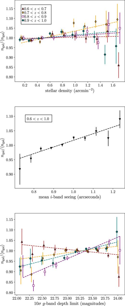
The galaxy density versus potential systematic relationship used to define weights that we apply to clustering measurements. Top panel: The galaxy density versus stellar density in four photometric redshift bins. The linear fits are used to determine the stellar contamination. The χ2 values for the fits are 9.7, 10.0, 3.5, and 14.3 (8 degrees of freedom). Middle panel: The galaxy density versus the mean i-band seeing for our full sample. The inverse linear fit is used to define weights applied to clustering measurements. The χ2 is 7.7 (8 degrees of freedom) and the coefficients are 0.788 and 0.0618. Bottom panel: The galaxy density versus g-band depth in four photometric redshift bins. The coefficients are interpolated as a function of redshift and used to define weights to be used in the clustering measurements. The χ2 values for the fits, given 8 degrees of freedom, are 7.7, 8.9, 12.7, and 6.1. The slopes are (−0.0256, 0.0320, 0.103, 0.0609).
Note that we repeat the fitting procedure for each photo |$z$| catalogue, hence redshift here means either |$z$|DNF–MOF or |$z$|BPZ–MOF. From Fig. 8, it seems that the measurements are a bit noisy. However, this procedure helps us resolve the peak in the stellar contamination of 5 per cent at ∼ 0.78. The uncertainty on each fit is ∼0.01, which is consistent with the scatter we find in the values of fstar per bin. The spline simply interpolates between the best-fitting values.
The dependencies we find are purely empirical as we lack any more fundamental understanding for how these correlations develop. They must result from the complicated intersection of our colour/magnitude selection and the photometric redshift algorithm, that are not perfectly captured by our mask. Besides the relations with different observing properties (airmass, seeing, dust, exposure time) are also very correlated what makes physical interpretation very complicated.
In the following section, we test the impact of these weights on the measured clustering and determine their total potential impact. In DES-BAO-MAIN, we show that the weights have minimal impact on the BAO scale measurements and that our treatment is thus sufficient for such measurements. Our treatment is not as comprehensive as Elvin-Poole et al. (2018), and thus further study might be required when using the sample defined here for non-BAO applications.
7 TWO-POINT CLUSTERING
In this section, we describe the basic two-point clustering properties of the samples previously defined. We concentrate on large scales where the BAO signal resides, and the sample using |$z$|DNF–MOF photometric redshifts that is the default one used in DES-BAO-MAIN.
The expected noise in the inverse covariance from the finite number of realizations (Hartlap, Simon & Schneider 2007) and the translation of that into the variance of derived parameters (Dodelson & Schneider 2013) is negligible given the size of our data vector (16 angular measurements per tomographic redshift bin) and the number of model parameters (one bias per bin). For instance, the increased error in derived best-fitting biases in any given bin would be subper cent. The change in the full |$\sqrt{\chi ^2}$| is |${\sim } 3.7{{\ \rm per\, cent}}$| (16 × 4 data points, see the discussion next). We therefore neglect these corrections in this section.
Fig. 9 shows the impact of the systematic weights on the measured angular clustering in terms of the difference Δ|$w$| between the pre-weighted correlation function |$w$| and the post-weighted one |$w$|weighted, relative to the statistical error σ|$w$| (i.e. neglecting all covariance). To compare this against the expected amplitude of the BAO feature at this scales, we also display in the thick solid black line the theoretical angular correlation function with and without BAO, for the second tomographic bin for concreteness, relative to the statistical errors. The corrections are all at the same level (or smaller) than the expected BAO signal.
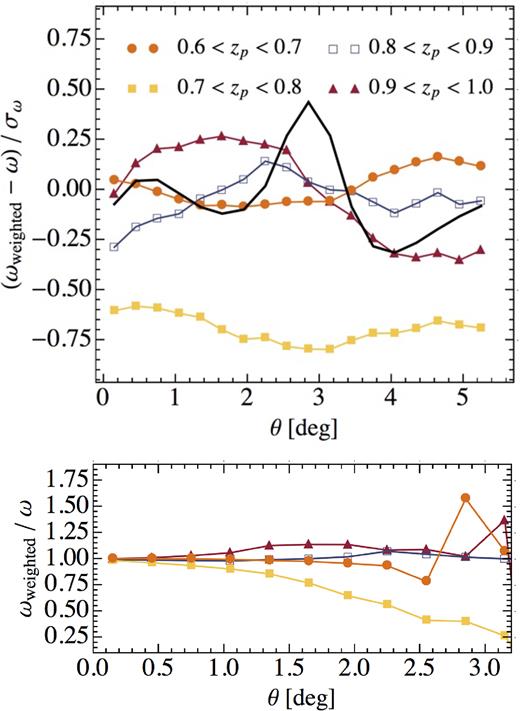
Top panel shows the impact of the systematic weights on each redshift bin, shown by the differential angular correlations, with and without weights applied, relative to the uncertainty. One can see that the weights make the biggest difference for the 0.7 < |$z$| < 0.8 bin, which is the redshift range with the greatest stellar contamination. The thick solid line displays the BAO feature in similar units, |$(w_{\rm BAO}-w_{\rm no\, BAO})/\sigma _w$|, for the second tomographic bin as an example (different bins show similar BAO strength but displaced slightly in the angular coordinate). The systematic weights only modify the underlying smooth shape and do not have a sharp feature at BAO scales. Bottom panel shows the ratio of correlations for each bin, which provides additional information on the absolute size of the corrections (in this case, we only plot up to scale with no zero crossings of |$w$|).
The weights have the largest impact in terms of clustering amplitude for the redshift bin 0.7 < |$z$| < 0.8, which is the redshift range with the largest stellar contamination (|${\sim } 4{{\ \rm per\, cent}}$|, see Table 2), although never exceeding one σ|$w$|. For the remaining bins, the change in the correlation functions are within 1/4 of σ|$w$|. We can assess quantitatively the total potential impact of the weights by calculating |$\chi _{\rm sys}^2=\Delta w(\theta) ^{t} C^{-1} \Delta w(\theta)$|; the square-root of this number is an upper bound in the impact, in terms of number of σ’s, that the weights could have on the determination of any model parameter.
In the range |$0.45\, {\rm deg} \lt \theta \lt 4.95\, {\rm deg}$|, with 16 data points, we find |$\chi _{\rm sys}^2=0.1, 1.35, 0.2$|, and 0.5, respectively, for each tomographic bin separately (showing that, for example, best-fitting bias derived solely from the second tomographic bin can be shifted by more than 1σ if weights are uncorrected for). More interestingly, for the four bins combined and including the full covariance matrix, we find |$\chi _{\rm sys}^2=1.35$|. This implies a maximum impact of 1.16σ in a derived global parameter such as the angular diameter distance measurement. This maximum threshold is well above the actual impact of the weights in DA/rs found in DES-BAO-MAIN, which is |$0.125 \sigma _{D_A/r_s}$| (see table 5 in that reference). We consider this an indication that the particular shape of the BAO feature is not easily reproducible by contaminants, and is therefore largely insensitive to such corrections, which is consistent with previous analyses (Ross et al. 2017b).
Fig. 10 displays the autocorrelation function (including observational systematic weights) of four tomographic bins of width Δ|$z$|photo = 0.1 between 0.6 ≤ |$z$|photo ≤ 1.0. Data at |$z$| > 0.8 appear to show significant BAO features. Best-fitting biases, derived 1σ errors and their corresponding χ2 values are reported as inset panels and in Table 2. The model displayed assumes linear theory and the MICE cosmology6 (Crocce et al. 2015; Fosalba et al. 2015), with an extra damping of the BAO feature, see DES-BAO-θ-METHOD for details. The χ2/dof are all of order ∼1 or better, showing that these are indeed good fits given the covariance of the data. In Table 2, we also report best-fitting bias values for a split of the sample into four tomographic bins using the BPZMOF photo |$z$|, showing no discrepancies.
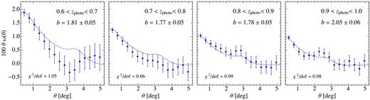
Angular correlation function in four redshift bins, for galaxies selected with |$z$|DNF–MOF. Symbols with error bars show the clustering of galaxy sample corrected for the most relevant systematics. The dashed line displays a model using linear theory with an extra damping of the BAO feature due to non-linearities and a linear bias fitted to the data (whose best-fitting value is reported in the inset labels). We consider 16 data points and one fitting parameter in each case (dof = 15). Note that the points are very covariant, which might explain the visual mismatch in the first tomographic bin that none the less retains a good χ2/dof.

Angular cross-correlation functions of the four tomographic bins in 0.6 < |$z$|photo < 1.0, see Fig. 10, for galaxies selected according to |$z$|DNF–MOF. The model prediction shown with the dashed lines assumes a bias equal to the geometric mean of the autocorrelation fits, i.e. |$b_{ij}=\sqrt{b_i b_j}$|, and is basically proportional to the overlap of redshift distributions, which are shown in the bottom right-hand panel.
Overall the cross-correlations show a good match to the model, which is sensitive to the tails of the redshift distributions and the geometric mean bias. The χ2/dof are ∼1. The non-adjacent bin 1 × 3 (where the expected clustering signal is negligible) shows an excess correlation on very large scales. This most probably indicates a residual systematic and not a problem of the photo z distributions.
The large χ2 values in some of the cross-correlations (bins 2 × 3 and 3 × 4) are driven by the non-diagonal structure of the covariance matrix, rather than a mismatch between the best-fitting bias of the cross-correlation bij compared to the geometrical mean of the autocorrelation biases. For example, for 2 × 3 the best-fitting bias from |$w$|2 × 3 is only |$2{{\ \rm per\ cent}}$| larger than |$\sqrt{b_2 b_3}$| (and the corresponding χ2 change subper cent). On the other hand, the χ2 of the cross-correlation drops to 0.4 if we only consider a diagonal covariance matrix. Similarly, |$\chi ^2_{3 \times 4}$| drops to 1.28 from 2 using a diagonal covariance matrix. Overall, we conclude there is a fairly good match between the implications of the overlap of redshift distributions and the cross-correlation clustering signal.
In Fig. 12, we show ξ(sperp) that is the 3D correlation function binned only in projected physical separations. To compute this correlation, we converted (photometric) redshift and angles to physical distances assuming MICE cosmology. This yields a 3D map of the galaxies in comoving coordinates. Random points are distributed in this volume with the same angular distribution as the angular mask defined in Section 5, and used for |$w$|(θ), and drawing redshifts randomly from the galaxies themselves. Pair counts are then computed and binned in projected separations. A full detail of such procedure is given in DES-BAO-MAIN as well as in Ross et al. (2017a). The modelling displayed in Fig. 12 projects the real space 3D correlation function into photometric space assuming Gaussian photometric redshift errors per galaxy, provided in Table 2 as σ68. It also assumes a linear bias between the galaxies and the matter field.
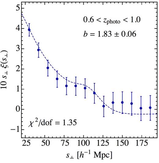
3D correlation function binned in projected pair separations. We use projected separations because radial pairs are damped due to photo |$z$| mixing. The dashed line is the best-fitting model assuming linear bias and a smeared BAO feature, as discussed in detail in DES-BAO-MAIN.
The bias recovered from the 3D projected clustering at a mean redshift of 0.8 is b = 1.83 ± 0.06, consistent with the one from |$w$|(θ) tomography. In addition, we stress that this clustering estimate includes all cross-correlations of the data. The fact that it is matched by the theory modelling, which in turn includes a characterization of the redshift distributions per galaxy, represents also an additional consistency check of reliability of the photometric redshifts.
8 CONCLUSIONS
This paper describes the selection of a sample of galaxies, optimized for BAO distance measurements, from the first year of DES data. By construction, this sample is dominated by red and luminous galaxies with redshifts in the range 0.6 < |$z$| < 1.0. We have extended the selection of red galaxies beyond that of previously published imaging data used for similar goals in SDSS by Padmanabhan et al. (2005) to cover the higher redshift and deeper data provided by DES.
We compute the expected magnitudes of galaxy templates in the four DES filters and identify the (i − |$z$|) and (|$z$| − i) colour space to select red galaxies in the redshift range of interest. The actual selection in colour and magnitude is defined using the BAO distance measurement figure-of-merit as a guiding criteria. Remarkably, the resulting forecast matches the results obtained in DES-BAO-MAIN with the final analysis. The global flux limit of the sample is iauto < 22, although we later introduce a sliding magnitude cut to limit ourselves to brighter objects towards lower redshifts.
We consider three different photo |$z$| catalogues, with two different photometric determinations. We showed that the typical photo |$z$| uncertainty (in units of 1 + |$z$|) goes from |$2.3{{\ \rm per\, cent}}$| to |$3.6{{\ \rm per\, cent}}$| from low to high redshift, for DNF redshifts using MOF photometry, and slightly worse for BPZ with MOF photometry. Hence, the former constitutes our primary catalogue in DES-BAO-MAIN, while the latter is used for consistency. Redshift estimations based on coadd photometry turned out to be worse than those derived from MOF photometry by |$10{{\ \rm per\, cent}}\text{--}20{{\ \rm per\, cent}}$|. Our final sample is made of 1.3 million red galaxies across 1336 deg2 of area, largely contained in one compact region (SPT).
We study and mitigate, when needed, observational systematics traced by various survey property maps. Of these, the most impactful is the stellar contamination, which we find none the less bound to |$\lt 4{{\ \rm per\, cent}}$|. Also i-band mean seeing and g-band depth are relevant. We define weights to be applied to the galaxies when computing pair counting to remove the relations between galaxy number density and large-scale fluctuations in those SPs. We show that none of these corrections have an impact on BAO measurements mainly because they can eventually modify the broad shape of the correlation functions but do not introduce a characteristic localized scale as the BAO.
Lastly, we characterized the two-point clustering of the sample, which is then used in DES-BAO-MAIN to derive distance constraints. We find the autocorrelations to be consistent with a bias that evolves only slightly with redshift, from 1.8 to 2. The bias derived from the tomographic analysis is consistent with the one fitted to the whole sample range with the 3D projected distance analysis. Furthermore, we investigate the cross-correlation between all the tomographic bins finding clustering amplitudes matching expectations, although with poor χ2-values in some cases. Overall, this is a further test of the assumed redshift distributions.
This paper serves the purpose of enabling for the first time BAO distance measurements using photometric data to redshifts |$z$| ∼ 1. These measurements achieve a precision comparable to those considered state of the art using photometric redshift to this point (Seo et al. 2012), as well as those from WiggleZ (Blake et al. 2011), which are both limited to |$z$| ∼ 0.65. These BAO results are presented in detail in DES-BAO-MAIN. While this paper was completed, the third year of DES data was made available to the collaboration, totalling three to four times the area presented here, and similar or better depth. Hence, we look forward to that analysis, which should already yield a very interesting counterpart to the high-precision low-|$z$| BAO measurements already existing.
ACKNOWLEDGEMENTS
MC acknowledges support from the Spanish Ramon y Cajal MICINN program. MC and EG have been partially funded by AYA2015-71825. AJR is grateful for support from the Ohio State University Center for Cosmology and AstroParticle Physics. KCC acknowledges the support from the Spanish Ministerio de Economia y Competitividad grant ESP2013-48274-C3-1-P and the Juan de la Cierva fellowship. This work has used CosmoHub, see Carretero et al. (2017). CosmoHub has been developed by the Port d’Informació Científica (PIC), maintained through a collaboration of the Institut de Física d’Altes Energies (IFAE) and the Centro de Investigaciones Energéticas, Medioambientales y Tecnológicas (CIEMAT) and was partially funded by the ‘Plan Estatal de Investigación Cientfica y Técnica y de Innovación’ program of the Spanish government.
We are grateful for the extraordinary contributions of our CTIO colleagues and the DECam Construction, Commissioning, and Science Verification teams in achieving the excellent instrument and telescope conditions that have made this work possible. The success of this project also relies critically on the expertise and dedication of the DES Data Management group.
Funding for the DES Projects has been provided by the U.S. Department of Energy, the U.S. National Science Foundation, the Ministry of Science and Education of Spain, the Science and Technology Facilities Council of the United Kingdom, the Higher Education Funding Council for England, the National Center for Supercomputing Applications at the University of Illinois at Urbana-Champaign, the Kavli Institute of Cosmological Physics at the University of Chicago, the Center for Cosmology and Astro-Particle Physics at the Ohio State University, the Mitchell Institute for Fundamental Physics and Astronomy at Texas A&M University, Financiadora de Estudos e Projetos, Fundação Carlos Chagas Filho de Amparo à Pesquisa do Estado do Rio de Janeiro,Conselho Nacional de Desenvolvimento Científico e Tecnológico and the Ministério da Ciência, Tecnologia e Inovação, the Deutsche Forschungsgemeinschaft, and the Collaborating Institutions in the DES.
The Collaborating Institutions are Argonne National Laboratory, the University of California at Santa Cruz, the University of Cambridge, Centro de Investigaciones Energéticas, Medioambientales y Tecnológicas-Madrid, the University of Chicago, University College London, the DES-Brazil Consortium, the University of Edinburgh, the Eidgenössische Technische Hochschule (ETH) Zürich, Fermi National Accelerator Laboratory, the University of Illinois at Urbana-Champaign, the Institut de Ciències de l’Espai (IEEC/CSIC), the Institut de Física d’Altes Energies, Lawrence Berkeley National Laboratory, the Ludwig-Maximilians Universität München and the associated Excellence Cluster Universe, the University of Michigan, the National Optical Astronomy Observatory, the University of Nottingham, The Ohio State University, the University of Pennsylvania, the University of Portsmouth, SLAC National Accelerator Laboratory, Stanford University, the University of Sussex, Texas A&M University, and the OzDES Membership Consortium.
Based in part on observations at Cerro Tololo Inter-American Observatory, National Optical Astronomy Observatory, which is operated by the Association of Universities for Research in Astronomy (AURA) under a cooperative agreement with the National Science Foundation.
The DESDM is supported by the National Science Foundation under Grant Numbers AST-1138766and AST-1536171. The DES participants from Spanish institutions are partially supported by MINECO under grants AYA2015-71825, ESP2015-66861, FPA2015-68048, SEV-2016-0588, SEV-2016-0597, and MDM-2015-0509, some of which include ERDF funds from the European Union. IFAE is partially funded by the CERCA program of the Generalitat de Catalunya. Research leading to these results has received funding from the European Research Council under the European Union’s Seventh Framework Program (FP7/2007-2013) including ERC grant agreements 240672,291329, and 306478. We acknowledge support from the Australian Research Council Centre of Excellence for All-sky Astrophysics (CAASTRO), through project number CE110001020.
This manuscript has been authored by Fermi Research Alliance, LLC under Contract No. DE-AC02-07CH11359 with the U.S. Department of Energy, Office of Science, and Office of High Energy Physics. The United States Government retains and the publisher, by accepting the article for publication, acknowledges that the United States Government retains a non-exclusive, paid-up, irrevocable, world-wide license to publish or reproduce the published form of this manuscript, or allow others to do so, for United States Government purposes.
This paper has gone through internal review by the DES collaboration. The DES publication number for this article is DES-2017-0305. The Fermilab pre-print number is FERMILAB-PUB-17-585.
Footnotes
In turn computed as merr = −2.5(Fluxerr/Flux)/log (10).
Photometric redshift errors lead to |${\bar{n}}_{\rm eff} P \lt 1$| in all cases explored.
The completeness of the VIPERS sample depends on galaxy type and has a colour pre-selection to exclude galaxies at |$z$| < 0.5. We have included all the suggested incompleteness factors (Scodeggio et al. 2016), but none the less have decided to use COSMOS–SVC as our fiducial validation set to avoid potential residuals.
This is a complementary calibration technique used for the construction of Y1GOLD using the distinct colour locus occupied by stars to perform relative additional calibration between bands.
We make this choice throughout the DES-Y1 BAO analysis because the MICE N-Body simulation was used to calibrate the Halogen mock galaxy catalogues. MICE cosmology assumes a flat concordance LCDM model with Ωmatter = 0.25, Ωbaryon = 0.044, ns = 0.95, σ8 = 0.8, and h = 0.7.
The best-fitting bias and error from the theory covariance or the mocks one are consistent with each other, however, the χ2 values are only so to about |$40{{\ \rm per\, cent}}$|.
REFERENCES
