


ABSTRACT
Molecular dynamics simulations are used to analyse the effects after 20 MeV sulfur ion impact into an ice mixture consisting of water, carbon dioxide, ammonia, and methanol. By using a so-called REAX, i.e., reactive, potential, the chemical processes occurring after the impact can be studied. Such impacts may occur in Jupiter’s magnetosphere, where energetic S ions originate from Io’s surface and irradiate ice surfaces of Jupiter’s moons, of comets or ice dust particles entering the magnetosphere. By segmenting the ion trajectory to smaller pieces that fit into our simulation box, we can follow the ion from its impact point at the surface down to the depth where it is stopped. Electronic stopping is modelled by a thermal track model; it is necessary to use a sufficiently small track radius R in order to be able to include the hot-chemistry reactions occurring in the track volume. We find that the number of dissociations and ensuing reactions scales approximately linearly with the deposited energy density. In consequence, the total number of molecules produced is approximately proportional to the impact energy. In addition, the most complex molecules are formed at the highest energy densities. Smaller molecules such as formaldehyde and hydrogen peroxide, in contrast, are produced all along the ion track.
1 INTRODUCTION
The planet Jupiter is in the focus of current space missions. NASA’s space probe JUNO (JUpiter Near-polar Orbiter) analyses, among other objectives, the high-energetic particles in the Jovian magnetosphere. In the next decade, ESA’ s JUICE (Jupiter Icy Moon Explorer) mission will visit the Galilean moons Europa, Ganymede, and Callisto for radar ranging and visual spectroscopy of their surfaces. These moons have icy surfaces. Constant irradiation by ions stored in the magnetosphere influences the surfaces and changes their composition (Klinger et al. 1985; Johnson et al. 1985; Johnson 1990, 2001; Gudipati & Castillo-Rogez 2013). The composition of ice surfaces is complex; they can be described as a mixture of water and various cryogenic gases that condensed outside of the Solar system’s snow line; among them carbon dioxide, methane, methanol, ammonia, and other molecular species (Allodi et al. 2013; Martins et al. 2013; Portugal et al. 2014).
Jupiter’s strong magnetic field creates a magnetosphere, which is giant in relation to all other planetary magnetospheres found in the Solar system, and hosts an intense radiation scenario (Paranicas et al. 2009). A comprehensive overview on the ions and their energy collected by all missions in the Jovian system (from Pioneer to GALILEO) is given in the PhD thesis of Radioti (2006). The dominant ions – as measured at the orbit of the moon Europa – are H, O, and S ions; the energy distributions show maxima at around 100 keV, but extend to beyond several tens of MeV. The unusual presence of sulfur ions originates from sputtering processes and volcanic eruptions on the moon Io; this element has been found incorporated into the surfaces of the other Galilean moons (Carlson et al. 2009) and is supposed to have been implanted there from the impact of magnetospheric sulfur ions. Ion irradiation of the ice surfaces gives rise to molecular dissociations and subsequent subsurface reactions. As proposed by Ehrenfreund et al. (2004), a wealth of product molecules opening the way to pre-biotic chemistry can be expected in these radiation activated environments.
The processes occurring under irradiation of ice surfaces by energetic ions have been studied hitherto by laboratory astrophysics experiments (Allodi et al. 2013; Rothard et al. 2017). Early studies by Gerakines, Schutte & Ehrenfreund (1996) showed that complex products are formed when irradiating methane, formaldehyde, methanol, and ammonia ices. Already soon thereafter it was verified that laboratory ice analogues containing or yielding methanol are comparable with the material detected by the observation of comets (Moore & Hudson 1998). The recent review by Rothard et al. (2017) summarizes experimental results that were obtained for various pure ices – among them |${\rm CO}$|, |${\rm CH_4}$|, |${\rm CH_3OH}$|, |${\rm CH_3COCH_3}$|, |${\rm C_6H_{12}}$|, |${\rm NH_3}$|, |${\rm CO_2}$|, |${\rm SO_2}$|, |${\rm H_2O}$|, and |${\rm CH_4}$| – and ice mixtures. This latter category is more relevant for realistic cosmic surfaces; among the ices studied are binary, ternary, and quaternary mixtures of various pure samples described above (Moore & Hudson 1998; Strazzulla 1999; Moore et al. 2007; Boduch et al. 2012; de Barros et al. 2014a,b; Muñoz Caro et al. 2014; Islam, Baratta & Palumbo 2014; Lv et al. 2014a; Augé et al. 2016; Kaňuchová et al. 2016). Besides ion irradiation, also thermal processes (Sandford & Allamandola 1993) and photochemical processes induced by ultraviolet (UV) irradiation of ice mixtures were investigated (Allamandola, Sandford & Valero 1988; Muñoz Caro & Schutte 2003; Nuevo et al. 2008).
Theoretical understanding of the processes occurring under ion irradiation of ice surfaces can be guided by atomistic simulations based on the method of molecular dynamics (MD). Modern interatomic interaction potentials allow to include the breaking and reformation of bonds into their description; these so-called REAX potentials (van Duin et al. 2001; Chenoweth, van Duin & Goddard III 2008; Liu et al. 2011) thus allow to study chemical reactions. We employed in previous studies such potentials (Monti et al. 2012) to study collisions of ice clusters (Anders & Urbassek 2013), the interaction of solar-wind ions with ice surfaces (Anders & Urbassek 2017), and the interaction of cosmic ray ions with ice grains (Mainitz, Anders & Urbassek 2016, 2017).
In this paper, we study the interaction of a high-energy (20 MeV) sulfur ion with an ice surface. During its slowing down, the stopping of the ion changes from an almost purely electronic-stopping regime to the nuclear stopping dominating below around 100 keV. In order to follow this change, we segment the ion trajectory in several pieces, in which we study the processes induced by the S ion at various energies. Our analysis will focus on the details of the production of molecular fragments and novel reaction products, as a function of the decreasing ion energy along its path inside the ice surface.
2 METHODS
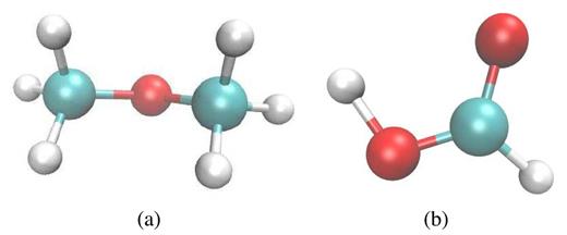
We use MD simulations to study the effect of S ion impact with an energy of 20 MeV into an ice surface. As target material we use a mixture of |${\rm H_2O}$|, |${\rm CO_2}$|, |${\rm NH_3}$|, |${\rm CH_3OH}$| in a 9.10:8.00:3.75:1.00 ratio, such as it has been proposed as a prototypical cometary ice mixture by Martins et al. (2013). In the upper energy range, the ion creates an ion track in the material such as it is shown schematically in Fig. 1(a). In the energy range considered by us, the ion suffers both electronic and nuclear energy losses. Data on the pertinent stopping powers of S ions as calculated by the srim software (Ziegler 2000) are assembled in Fig. 1(b). Above around 200 keV, electronic stopping dominates the losses, while nuclear stopping is predominant at lower energies. Nuclear stopping is maximum at around 13.5 keV, and electronic stopping at around 22.5 MeV. For comparison, also the stopping data in a pure water ice target are displayed in Fig. 1(b). We observe a close agreement of stopping in water and in our mixture, both in the positions of the maxima and in the absolute sizes of stopping powers.
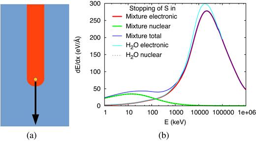
(a) Schematics of an ion producing a track. (b) Stopping power dE/dx of an S ion in a cometary ice mixture and in pure water. In addition to the electronic and nuclear contributions, the total stopping is displayed for the mixture. Data evaluated with Trim (Ziegler 2000).
Interactions are modelled using a reactive potential with the parameters published by Monti et al. (2012). Towards higher energies the Ziegler–Biersack–Littmark potential (Ziegler, Biersack & Littmark 1985) has been added to model the repulsive short-range interaction governing high-energy collisions, as described in detail previously (Anders & Urbassek 2013). We note that this potential has been employed already previously to study energetic impacts into ice surfaces (Anders & Urbassek 2013; Mainitz et al. 2016, 2017; Anders & Urbassek 2017). The ice mixture is generated in amorphous form by using Packmol (Martínez et al. 2009); after preparation, its structure is relaxed in a 4.8 ps simulation run to get rid of energetically unfavourable molecular positions and orientations. Then, the target is slowly heated to a temperature of 100 K. Our target assumes a density of 1.09 g m−3; in previous work we showed that the amorphous structure is stable (Anders & Urbassek 2017). The total number of atoms amounts to 955 866 atoms; the atomic number density is n = 77.6 atoms nm−3.
We use the lammps software (Plimpton 1995) to perform the simulations. We pursue the simulations until the number of dissociated fragments and reaction products formed do not change further in time; this may take up to 60 ps.
2.1 Segmenting the ion trajectory
Using srim (Ziegler 2000), the expected depth for S at 20 MeV is 11.66 ± 0.41 |$\mu$|m. The construction of a target that contains the entire ion trajectory exceeds by far today’s computational capabilities. We attack this problem by subdividing the ion trajectory into several segments; the processes in each segment are studied in a separate simulation. In detail, we consider a sulfur ion with energy E to enter a virgin simulation box filled with ice; we follow the ion trajectory until it leaves the simulation box and all subsequent processes in the box. The list of energies E simulated is provided in Table 1. Fig. 2 displays at which depth below the surface the S ion has been stopped to energy E such that the corresponding MD simulation applies.
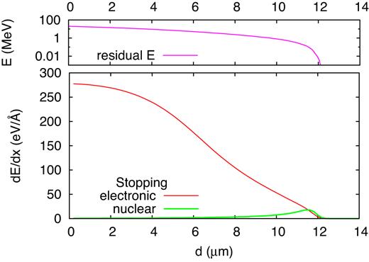
Electronic and nuclear stopping power dE/dx (lower panel), and residual energy E (upper panel), of a 20-MeV S ion as a function of the distance d passed in a cometary ice mixture. Note the logarithmic energy scale in the upper panel. Data evaluated as an average of 67 trajectories with srim (Ziegler 2000).
Simulated ion energies E, and corresponding velocities v. The ion range r and the (initial) electronic-stopping power, (dE/dx)e, were calculated using srim (Ziegler 2000). The track temperature, ΔT, is evaluated using equation (3). Ndiss and Nprod are the number of dissociated molecules and of novel molecules, respectively, as determined from our simulations. Ee and En denote the energy deposited in the simulation box in the electronic system and in recoil motion, respectively, while Edep is their sum. For ion energies below 13.5 keV the total energy is deposited inside the simulation volume.
| E (keV) | v (km s−1) | r (nm) | (dE/dx)e (eV Å−1) | ΔT (K) | Ndiss | Nprod | Ee (keV) | En (keV) | Edep (keV) |
|---|---|---|---|---|---|---|---|---|---|
| 20000 | 11000 | 11660 | 278 | 176000 | 3672 | 5284 | 87 | 1.0 | 88 |
| 10000 | 7748 | 7900 | 243 | 154000 | 2534 | 3573 | 61.5 | 0.5 | 62 |
| 2500 | 3900 | 3740 | 100 | 63000 | 1097 | 1836 | 31 | 0.4 | 31.4 |
| 1000 | 2450 | 1980 | 56.9 | 36000 | 901 | 1235 | 19.4 | 1.6 | 21.0 |
| 100 | 775 | 213 | 17.7 | 11100 | 212 | 274 | 6 | 1.2 | 7.2 |
| 25 | 388 | 56 | 9.64 | 6120 | 634 | 797 | 2.8 | 7.1 | 9.9 |
| 13.5 | 285 | 33 | 7.08 | 4500 | 935 | 1181 | 1.3 | 12.2 | 13.5 |
| 10.1 | 246 | 26 | 6.25 | 3970 | 728 | 947 | 1.3 | 8.8 | 10.1 |
| 2.3 | 163 | 9.1 | 3.00 | 1900 | 161 | 206 | 0.3 | 2.0 | 2.3 |
| 1 | 77.5 | 5.5 | 1.93 | 1220 | 83 | 107 | 0.07 | 0.93 | 1.0 |
The target has an extension of 202 × 202 × 312 Å3; periodic boundary conditions are applied in all directions. The ion starts in perpendicular direction along the longest direction of the box. Its initial temperature is set to 100 K, as appropriate for the surface temperature of Jupiter’s moon Europa (Carlson et al. 2009); during the simulations a Berendsen thermostat is used to cool the lateral boundaries in a zone of width 12 Å to this temperature in order to mimic heat conduction to the surroundings.
Note that when the ion energy falls below around 13.5 keV, the ion trajectory is fully contained in the simulation box; these simulations thus provide a full view into the final stages of ion stopping in the target.
For an ion energy above 13.5 keV, the ion will traverse the simulation box and leave it; we then do not follow the ion motion any longer, but restrict our attention to the processes occurring in the simulation box that are caused by the energy deposited by the projectile ion in it.
2.2 Electronic stopping

The energy lost by to the electronic system is recovered eventually as thermal energy. In our simulation, we assume that this occurs immediately after passage of the ion, such that a cylindrical track volume around the ion trajectory is homogeneously energized. This procedure is common practice in the MD modelling of ion track physics (Urbassek, Kafemann & Johnson 1994; Bringa & Johnson 2002; Pakarinen et al. 2009; Mainitz et al. 2016; Peña-Rodríguez et al. 2017). The actual physics of energy deposition in the track is, however, more complicated (Fleischer, Price & Walker 1975; Schiwietz et al. 2004; Toulemonde et al. 2006). The ionizing projectile ion creates fast electrons (so-called δ-electrons), which spread the energy in an fs time-scale around the ion path. The radial profile of the energy deposition around the ion path has been studied using Monte Carlo simulation (Gervais & Bouffard 1994) and roughly follows a 1/r2 distribution (Waligorski, Hamm & Katz 1986). The thermalization of the electrons and the energy transfer to the atomic system can be described fairly well in metallic systems, where electron–phonon coupling allows for a fast energy transfer (Toulemonde et al. 2006). In insulating materials, however, the electronic band gap prevents efficient energy exchange between the electronic and the atomic systems such that long-lived electronic excitations can survive. An early study of cosmic ray interaction with ice grains (Leger, Jura & Omont 1985) describes the processes after passage of the ion by the creation of δ-electrons, electron collision cascades and slowing down, creation of electron–hole pairs and their recombination, and the production of optical phonons; during this last step, finally the energy has been converted to atomic system.
The influence of the temporal and spatial structures of the electronic energy deposition around the ion trajectory on the track evolution has been studied using MD simulation with a focus on sputtering events (Beuve et al. 2003; Mookerjee et al. 2008). There it was established that sputtering decreases for long delay times and for extended energy deposition profiles, i.e. at low-energy densities. Similar effects can be assumed to occur for chemical reactions. Note that also the inclusion of the electric field that is established between the negatively charged expanding electron cloud and the remaining positive track core needs be included in the simulation (Cherednikov, Sun & Urbassek 2013).
Recent approaches to model the chemistry of ionizing radiation in solids (Chang & Herbst 2014; Shingledecker, Le Gal & Herbst 2017; Shingledecker & Herbst 2018) use Monte Carlo simulation to model the ion slowing down but also the transport of electrons in insulating matter. Chemistry is then included by a series of rate equations. So far such treatments have been restricted to relatively simple molecular solids such as frozen O2 and water ice (Shingledecker et al. 2017; Shingledecker & Herbst 2018).
2.3 Detectors
We identify molecules in our target with the help of a molecule detector (Anders & Urbassek 2013). It is based on Stoddard’s cluster detection algorithm (Stoddard 1978), which decides by a distance criterion (1.7 Å) whether atoms belong to the same molecule. An exception is made for the element H, where the distance limit is reduced to 1.28 Å in order to avoid false giant molecules.
3 RESULTS
3.1 Overview: molecular dissociations and novel molecular species
We first discuss summarily the number of dissociations and product molecules formed in the simulations performed with our various projectile energies. Here, we identify the number of ‘dissociations’, Ndiss, as the number of destroyed molecules, and the number of ‘novel molecules’, Nprod, as any molecular (or atomic) species not present before. Note that these novel molecules include both fragments and reaction products.
We relate these numbers to the total energy deposited in the simulation box, Edep. If the ion leaves the simulation box – this happens for energies E > 13.5 keV – then its loss in kinetic energy equals Edep; if it is stopped in the simulation box, then Edep = E.
Fig. 4 shows the number of dissociated original molecules and new molecular products as a function of the deposited energy. In order to check whether the electronic part of the deposited energy, Ee, or the total deposited energy, Edep, correlates better with these numbers, we provide plots of the dependence on both quantities. It shows up that the correlation with total deposited energy is more reliable so that we will restrict the discussion to Fig. 4(a). Towards large deposited energies, above around 20 keV, the correlations with Edep and Ee are equally satisfactory; this occurs for ion energies above 1 MeV, where stopping is dominated by electronic losses. At small energies, E ≲ 100 keV, on the other hand, electronic energy loss is not sufficient to heat the track atoms sufficiently for bond breaks, cf. Table 1, and hence the correlation with the total deposited energy is more satisfactory. Note that deposited energy does not grow monotonically with the ion energy E, see Table 1 and Fig. 1(b), in contrast to Ee.
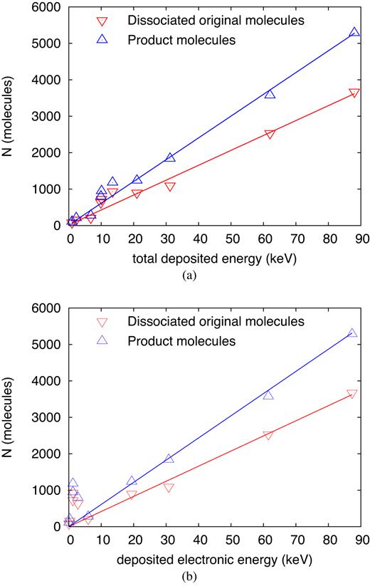
Number of dissociations and of product molecules as a function of (a) the total energy, Edep, and (b) the electronic energy, Ee, deposited by the ion in the simulation volume. Lines denote linear fits, equation (5).
Towards smaller energies, systematic deviations from the linear law, equation (5), show up. Most pronounced is an increase of dissociations and products at deposited energies of around 14 keV. From Table 1, we see that this occurs at energies close to the maximum of nuclear stopping power, see Fig. 1(b) at 13.5 keV. Finally, towards smaller deposited energies the numbers of dissociations and products falls off more steeply than the linear law, equation (5), predicts.
In the following, the effects of the sulfur ion are described beginning with the initial energy of 20 MeV.
3.2 Sulfur ion at 20 MeV
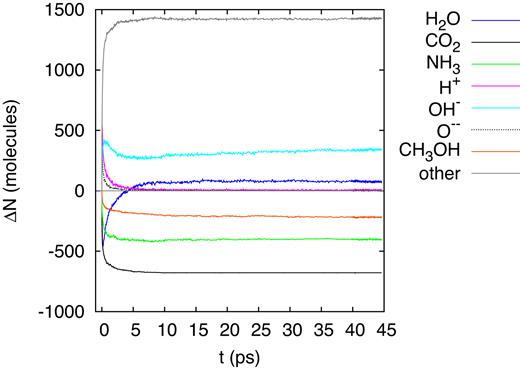
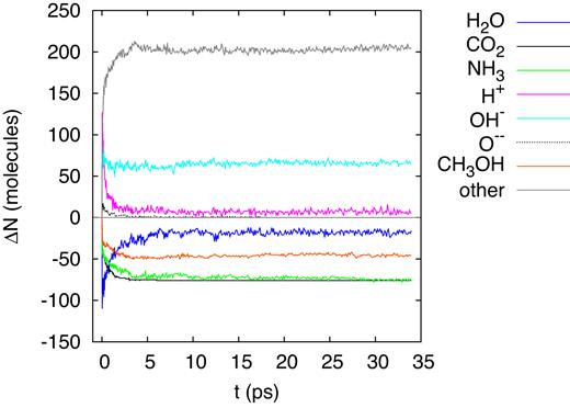
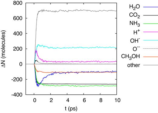
A 20-MeV sulfur ion generates a straight ion track extending throughout the entire simulation box; the ion loses the main part of its energy by electronic stopping and only a small part by nuclear collisions. Fig. 5 displays the changes in the number of original molecules (|${\rm H_2O}$|, |${\rm CO_2}$|, |${\rm NH_3}$|, and |${\rm CH_3OH}$|) and of several major fragments (H, O, and OH). The dissociations and reactions have terminated within 10 ps, and the numbers of original molecules and fragments are stable after that time. With the exception of water, the number of the original molecules is reduced in comparison to the original state; the net production of water molecules is evidence of reactions occurring – in particular in the time of > 5 ps after track formation – that result in water formation. The number of dissociated |${\rm CO_2}$| molecules is particularly high; indeed it is of the order of molecules in the track itself (Ntrack = 1801). This demonstrates that the dissociation region extends beyond the track radius.
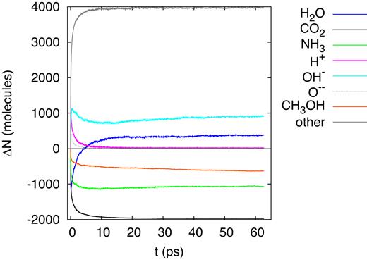
Evolution of the change in the number of molecules, ΔN, in the simulation box for an ion energy of 20 MeV.
Water shows a peculiar behaviour in that after the early dissociations, water molecules are reformed and the number of water molecules increases again; this behaviour was already seen in previous irradiation simulations of ice mixtures (Anders & Urbassek 2017; Mainitz et al. 2016). However, in the present simulation, the final water abundance even surpasses the original one. Note that after around 15 ps, the number of free H atoms has decreased to zero; due to their high mobility, all H atoms have found reaction partners. Free O atoms have recombined even earlier, before 10 ps. OH radicals, on the other hand, are still abundant in the simulation volume and may survive.
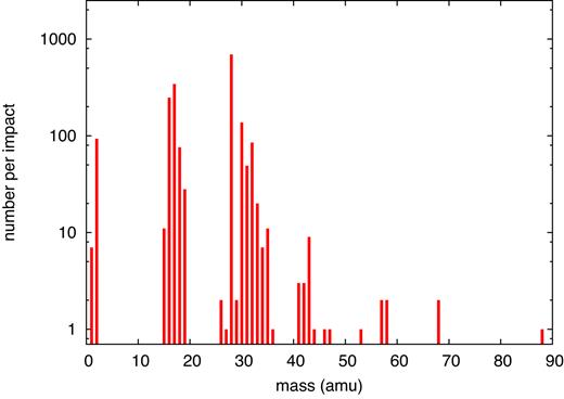
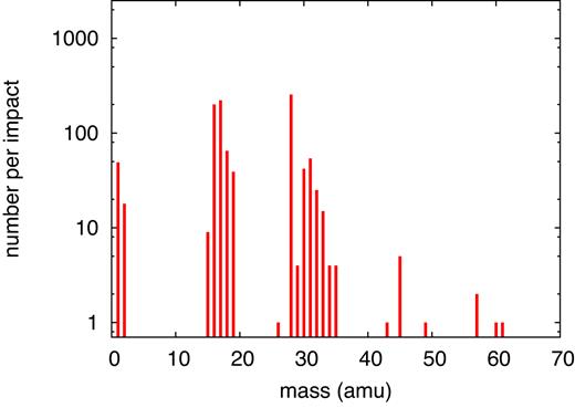
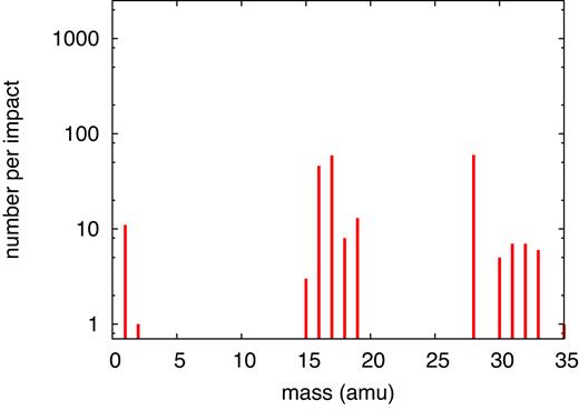
Table 2 provides a compilation of all products formed in this simulation; the pertinent mass spectrum is displayed in Fig. 6. The original ice mixture features masses only at 17 (|${\rm NH_3}$|), 18 (|${\rm H_2O}$|), 32 (|${\rm CH_3OH}$|), and 44 amu (|${\rm CO_2}$|); these molecules are excluded from the presentation in Fig. 6. In the product mass spectrum, the mass regions around the original molecules appear broadened in the windows of 15–20, 30–35, and 40–45 amu; the species there in part represent original molecules to which an H has been added or subtracted. The most frequent products are |${\rm CO}$|, |${\rm OH}$|, and |${\rm NH_2}$|. Major and important products are formaldehyde (|${\rm CH_2O}$|), and molecular oxygen and hydrogen.
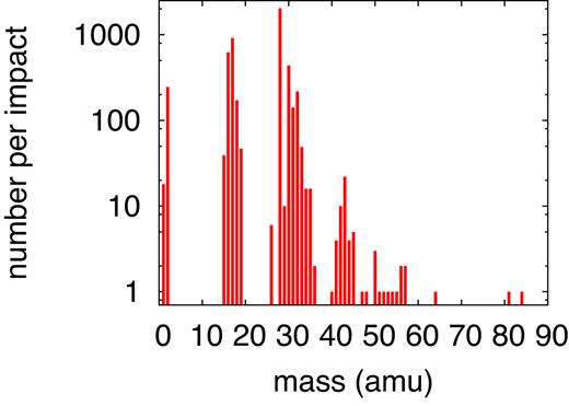
Simulated mass spectrum of molecular products found for an ion energy of 20 MeV.
Molecular products formed at an ion energy of 20 MeV. The table is ordered by molecules containing C but no N, containing no C but N, and containing neither C nor N; in each of these blocks they are listed in the order of increasing complexity.
| Sum formula | Mass (u) | Amount |
|---|---|---|
| |${\rm CO}$| | 28 | 2037 |
| |${\rm CNO}$| | 42 | 3 |
| |${\rm CHO}$| | 29 | 3 |
| |${\rm CHO_2}$| | 45 | 4 |
| |${\rm CHNO}$| | 43 | 22 |
| |${\rm CH_2O}$| | 30 | 287 |
| |${\rm CH_2N}$| | 28 | 2 |
| |${\rm CH_2NO}$| | 44 | 4 |
| |${\rm CH_3}$| | 15 | 8 |
| |${\rm CH_3O}$| | 31 | 141 |
| |${\rm CH_3N}$| | 29 | 6 |
| |${\rm CH_3NO}$| | 45 | 1 |
| |${\rm CH_4}$| | 16 | 13 |
| |${\rm CH_4N}$| | 30 | 3 |
| |${\rm CH_5O}$| | 33 | 6 |
| |${\rm CH_6O_2}$| | 50 | 3 |
| |${\rm CH_6N}$| | 32 | 1 |
| |${\rm C_2O}$| | 40 | 1 |
| |${\rm C_2HO}$| | 41 | 4 |
| |${\rm C_2HO_2}$| | 57 | 2 |
| |${\rm C_2HNO}$| | 55 | 1 |
| |${\rm C_2H_2}$| | 26 | 6 |
| |${\rm C_2H_2O}$| | 42 | 7 |
| |${\rm C_2H_2NO}$| | 56 | 2 |
| |${\rm C_2H_6}$| | 30 | 1 |
| |${\rm C_3O}$| | 52 | 1 |
| |${\rm C_3O_3}$| | 84 | 1 |
| |${\rm C_3HO}$| | 53 | 1 |
| |${\rm C_3H_2O}$| | 54 | 1 |
| |${\rm C_4HO_2}$| | 81 | 1 |
| |${\rm NO}$| | 30 | 147 |
| |${\rm NH}$| | 15 | 31 |
| |${\rm NHO}$| | 31 | 1 |
| |${\rm NHO_2}$| | 47 | 1 |
| |${\rm NH_2}$| | 16 | 610 |
| |${\rm NH_2O}$| | 32 | 9 |
| |${\rm NH_2O_2}$| | 48 | 1 |
| |${\rm NH_2O_3}$| | 64 | 1 |
| |${\rm NH_3O}$| | 33 | 35 |
| |${\rm NH_4}$| | 18 | 172 |
| |${\rm NH_4O}$| | 34 | 7 |
| |${\rm NH_5O}$| | 35 | 1 |
| |${\rm NH_5O_2}$| | 51 | 1 |
| |${\rm N_2}$| | 28 | 1 |
| |${\rm N_2H}$| | 29 | 1 |
| |${\rm N_2H_2}$| | 30 | 1 |
| |${\rm H}$| | 1 | 18 |
| |${\rm H_2}$| | 2 | 246 |
| |${\rm O}$| | 16 | 1 |
| |${\rm OH}$| | 17 | 915 |
| |${\rm H_3O}$| | 19 | 47 |
| |${\rm O_2}$| | 32 | 208 |
| |${\rm O_2H}$| | 33 | 8 |
| |${\rm H_2O_2}$| | 34 | 9 |
| |${\rm HOH} \cdots {\rm OH}$| | 35 | 15 |
| 2|${\rm H_2O}$| | 36 | 2 |
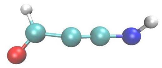
True products are found in the mass region beyond 50 amu, and feature molecules such as |${\rm C_2H_2NO}$| or |${\rm C_3H_2O}$|. We visualize several of these interesting molecules in Fig. 7. Among them is buthyne-dione which constitutes the molecule with the longest carbon chain formed (containing 4 C atoms), which contains two aldehyde groups with one proton missing. Two other molecules are remarkable because they contain C rings: cyclopropan-trione and the radical of cyclopropanone. These unusual molecules might be unstable leading to further reactions on time-scales beyond our simulation time. We conclude that 20 MeV S irradiation of an ice mixture may form complex products close to the surface, from which they might also be emitted by sputtering to the vacuum above it.
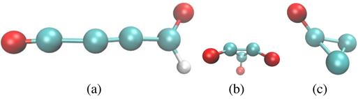
Interesting reaction products found for an ion energy of 20 MeV: (a) buthyne-dione-radical, |${\rm C_4HO_2}$|, (b) cyclopropan-trione, |${\rm C_3O_3}$|, and (c) radical of cyclopropanone, |${\rm C_3O}$|.
Hydrogen peroxide, |${\rm H_2O_2}$| and molecular oxygen, hydrogen, and |${\rm HO_2}$| are formed, as in all simulations down to an ion energy of 10 keV. These species have been taken as an indicator of radiolysis on ice surfaces (Gudipati & Castillo-Rogez 2013): they have in fact been found in the radiative environment of Jupiter’ s moons (Carlson et al. 2009) and were taken as a sign that further interesting products of radiolysis may be present there (Chela-Flores 2006). While the hydrogen as volatile gas will evaporate and escape from the moons’ gravitational field, oxygen might contribute to a faint atmosphere (Carlson et al. 2009).
Shortly after passage of the ion, the hot and highly pressurized ion track volume expands radially outward creating a cylindrical compression wave, in the course of which the track density becomes considerably reduced. We present the radial distribution of the density as a function of time after ion passage in Fig. 8; the data have been averaged along the track axis and in azimuthal direction (Mainitz et al. 2016). Even up to the end of the simulation, the track core remains underdense due to the high temperatures still present there, 980 K at the end of the simulation (at 62.7 ps after impact). However, reactions have terminated, as Fig. 5 shows; at least they have reached an equilibrium in which no new species are formed. An inspection of the location where the reaction products and fragments have been produced shows that nearly all of them took place within or close to the hot track, either by direct hits by the projectile ion or by the high temperatures imparted by the electronic-stopping process.
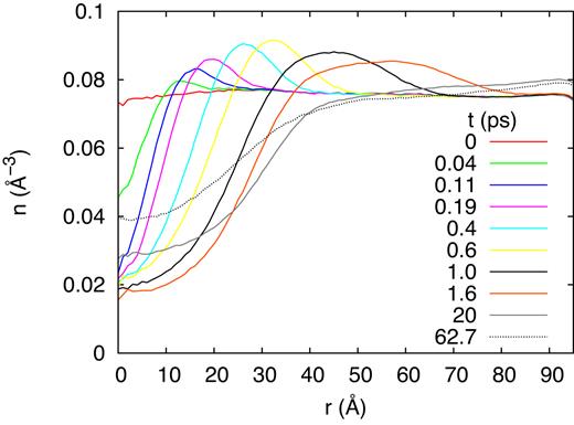
Lateral compression wave initiated by the track of a 20 MeV ion: time evolution of the radial density profile.
3.3 Sulfur ion at 2.5 MeV
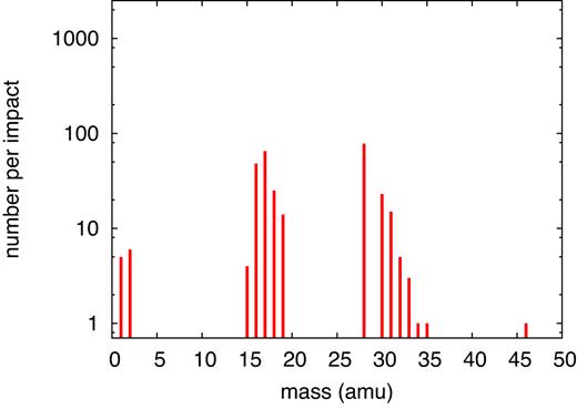
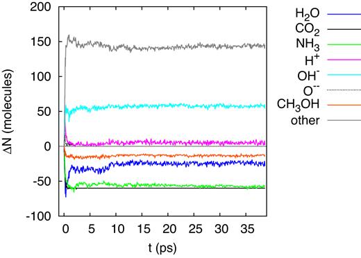
After traversing around 8 |$\mu$|m of the target the projectile energy has degraded to 2.5 MeV, cf. Table 1 and Fig. 2. The differences to the higher energy (20 MeV) track show up mainly in the reduced numbers of reaction products that are formed, as is evidenced by the shorter and less populated table of products, Table 3, and by the smaller number of dissociations monitored in Fig. 9. These reductions are a consequence of the smaller stopping power at this lower energy. Similarly, the mass spectrum of the products formed (Fig. 10), is not as rich as for the higher energy, 20 MeV, see Fig. 6. Here, formaldehyde and other radiolytic products such as |${\rm CO}$|, |${\rm OH}$|, and |${\rm H_2O_2}$| are still generated but in reduced numbers, making the distributions in the mass spectrum somewhat narrower and smaller. Fig. 11 exemplifies the reaction products formed by showing the most complex molecule synthesized at this energy, the radical of propyne-amine-aldehyde, which is based on a carbon chain of 3 C atoms, while in the case of 20 MeV we observed carbon chains containing 4 C atoms.
Evolution of the change in the number of molecules, ΔN, in the simulation box for an ion energy of 2.5 MeV.
Simulated mass spectrum of molecular products found for an ion energy of 2.5 MeV.
Propyne-amine-aldehyde radical, |${\rm COHC_2NH}$|: an interesting reaction product found for an ion energy of 2.5 MeV.
Molecular products formed at an ion energy of 2.5 MeV.
| Sum formula | Mass (u) | Amount |
|---|---|---|
| |${\rm CO}$| | 28 | 693 |
| |${\rm CNO}$| | 42 | 1 |
| |${\rm CHO}$| | 29 | 2 |
| |${\rm CHN}$| | 27 | 1 |
| |${\rm CHNO}$| | 43 | 9 |
| |${\rm CH_2O}$| | 30 | 88 |
| |${\rm CH_2O_2}$| | 46 | 1 |
| |${\rm CH_2NO}$| | 44 | 1 |
| |${\rm CH_3}$| | 15 | 2 |
| |${\rm CH_3O}$| | 31 | 45 |
| |${\rm CH_4}$| | 16 | 7 |
| |${\rm CH_5O}$| | 33 | 13 |
| |${\rm CH_3NH_2}$| | 31 | 1 |
| |${\rm C_2HO}$| | 41 | 3 |
| |${\rm C_2HO_2}$| | 57 | 2 |
| |${\rm C_2H_2}$| | 26 | 2 |
| |${\rm C_2H_2O}$| | 42 | 2 |
| |${\rm C_2H_2O_2}$| | 58 | 2 |
| |${\rm C_3O_2}$| | 68 | 1 |
| |${\rm C_3HO}$| | 53 | 1 |
| |${\rm C_3H_2NO}$| | 68 | 1 |
| |${\rm NO}$| | 30 | 49 |
| |${\rm NH}$| | 15 | 9 |
| |${\rm NHO}$| | 31 | 3 |
| |${\rm NHO_2}$| | 47 | 1 |
| |${\rm NH_2}$| | 16 | 241 |
| |${\rm NH_2O}$| | 32 | 3 |
| |${\rm NH_3O}$| | 33 | 6 |
| |${\rm NH_4}$| | 18 | 76 |
| |${\rm H}$| | 1 | 7 |
| |${\rm H_2}$| | 2 | 93 |
| |${\rm OH}$| | 17 | 343 |
| |${\rm H_3O}$| | 19 | 28 |
| |${\rm O_2}$| | 32 | 82 |
| |${\rm O_2H}$| | 33 | 1 |
| |${\rm H_2O_2}$| | 34 | 7 |
| |${\rm HOH}\cdots{\rm OH}$| | 35 | 11 |
| 2|${\rm H_2O}$| | 36 | 1 |
3.4 Sulfur ion at 100 keV
When the ion energy has slowed down to 100 keV, the total stopping power has further been reduced, see Fig. 1(b); however, now the contribution of nuclear stopping has increased such that now electronic and nuclear stopping contribute approximately equally. Compared to the 20-MeV simulation, the stopping power has been reduced roughly by an order of magnitude, and so has the energy deposited in the simulation volume, see Table 1. Consequently, the number of dissociations and products formed are also reduced by a factor of around 10, as evidenced in Fig. 12. The list of species produced (Table 4) has become considerably shortened, and the simulated mass spectrum, Fig. 13, is less complex than for the previous cases shown. While the common fragment molecules such as |${\rm CO}$|, |${\rm OH}$|, and |${\rm NH_2}$| are still present, |${\rm H_2O_2}$| and other radiolytic products become rarer.
Evolution of the change in the number of molecules, ΔN, in the simulation box for an ion energy of 100 keV.
Simulated mass spectrum of molecular products found for an ion energy of 100 keV.
Molecular products formed at an ion energy of 100 keV.
| Sum formula | Mass (u) | Amount |
|---|---|---|
| |${\rm CO}$| | 28 | 78 |
| |${\rm CHO}$| | 29 | 1 |
| |${\rm CH_2O}$| | 30 | 23 |
| |${\rm CH_2O_2}$| | 46 | 1 |
| |${\rm CH_3}$| | 15 | 4 |
| |${\rm CH_3O}$| | 31 | 14 |
| |${\rm CH_4}$| | 16 | 1 |
| |${\rm CH_5O}$| | 33 | 2 |
| |${\rm CH_6O_2}$| | 50 | 1 |
| |${\rm CH_6N}$| | 32 | 1 |
| |${\rm C_2H_6O}$| | 46 | 1 |
| |${\rm NHO}$| | 31 | 1 |
| |${\rm NH_2}$| | 16 | 48 |
| |${\rm NH_3O}$| | 33 | 1 |
| |${\rm NH_4}$| | 18 | 25 |
| |${\rm H}$| | 1 | 5 |
| |${\rm H_2}$| | 2 | 6 |
| |${\rm OH}$| | 17 | 65 |
| |${\rm H_3O}$| | 19 | 14 |
| |${\rm O_2}$| | 32 | 5 |
| |${\rm H_2O_2}$| | 34 | 1 |
| |${\rm HOH}\cdots{\rm OH}$| | 35 | 1 |
Two interesting reaction products that have been generated are an ether, |${\rm H_3C-O-CH_3}$|, that formed by the reaction of two methanol molecules (Fig. 14a), and formic acid (Fig. 14b). The latter molecule constitutes the simplest organic acid that was not present initially. Another interesting product molecule is the protonated methanol molecule |${\rm H_3C-O-H_2}$| which we observe down to the lowest irradiation energy. This unstable molecule has been seen – together with protonated formaldehyde, |${\rm CH_3O}$| – on comet Halley (Geiss et al. 1991).
Interesting reaction products found for an ion energy of 100 keV: (a) dimethyl ether, |${\rm H_3C-O-CH_3}$|, and (b) formic acid, |${\rm CH_2O_2}$|.
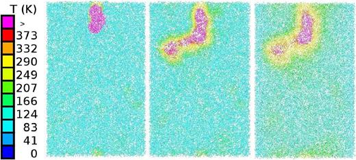
For this ion energy, we visualize the time evolution of the track formed by the ion. Fig. 15 shows a straight track structure from which the initially high temperatures diffuse radially outwards; after a time of around 33 ps, the temperatures have fallen to around 290 K, and are thus close to the freezing point of water. After this time, temperatures will continue decreasing such that eventually all species in the track will be frozen again.
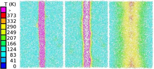
Cross-section through the track of a 100 keV ion at times of 0.047 ps (left), 1.7 ps (middle), and 33.4 ps (right). Colour codes local temperature, see colour bar.
3.5 Sulfur ion at 10 keV
As Table 5 and Fig. 16 demonstrate, the number and diversity of products increases for this small impact energy in comparison to the case of 100 keV. This is caused by the increasing influence of nuclear energy loss, which has now become dominant, cf. Fig. 1(b), which shows that this energy is close to the maximum of nuclear energy loss. The ion range has now become smaller than the length of the simulation volume (Table 1). The snapshots of the track structure (Fig. 17) show how due to scattering of the projectile ion and generation of energetic recoils, a collision cascade forms, which leads to strong deviations from the linear-track scenario holding at higher ion energies (Fig. 15).
Simulated mass spectrum of molecular products found for an ion energy of 10 keV.
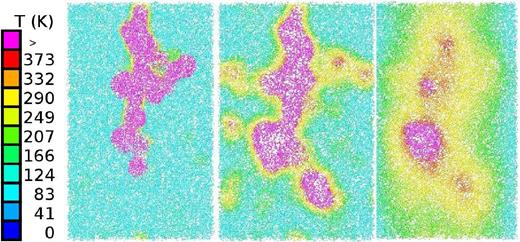
Cross-section through the collision cascade set up by a 10 keV ion at times of 0.091 ps (left), 1.97 ps (middle), and 33.3 ps (right). Colour codes local temperature, see colour bar.
Molecular products formed at an ion energy of 10 keV.
| Sum formula | Mass (u) | Amount |
|---|---|---|
| |${\rm CO}$| | 28 | 254 |
| |${\rm CO_3}$| | 60 | 1 |
| |${\rm CN}$| | 26 | 1 |
| |${\rm CHO}$| | 29 | 3 |
| |${\rm CHO_2}$| | 45 | 4 |
| |${\rm CHO_3}$| | 61 | 1 |
| |${\rm CHNO}$| | 43 | 1 |
| |${\rm CH_2O}$| | 30 | 38 |
| |${\rm CH_2N}$| | 28 | 1 |
| |${\rm CH_3}$| | 15 | 4 |
| |${\rm CH_3O}$| | 31 | 54 |
| |${\rm CH_3N}$| | 29 | 1 |
| |${\rm CH_3NO}$| | 45 | 1 |
| |${\rm CH_4N}$| | 30 | 2 |
| |${\rm CH_5O}$| | 33 | 8 |
| |${\rm CH_5O_2}$| | 49 | 1 |
| |${\rm CH_3NH_3}$| | 32 | 2 |
| |${\rm C_2HO_2}$| | 57 | 2 |
| |${\rm NO}$| | 30 | 2 |
| |${\rm NH}$| | 15 | 5 |
| |${\rm NHO}$| | 31 | 1 |
| |${\rm NH_2}$| | 16 | 199 |
| |${\rm NH_2O}$| | 32 | 2 |
| |${\rm NH_2OH}$| | 33 | 6 |
| |${\rm NH_4}$| | 18 | 65 |
| |${\rm H}$| | 1 | 49 |
| |${\rm H_2}$| | 2 | 18 |
| |${\rm O}$| | 16 | 1 |
| |${\rm OH}$| | 17 | 222 |
| |${\rm H_3O}$| | 19 | 39 |
| |${\rm O_2}$| | 32 | 21 |
| |${\rm O_2H}$| | 33 | 1 |
| |${\rm H_2O_2}$| | 34 | 4 |
| |${\rm HOH}\cdots{\rm OH}$| | 35 | 4 |
Also the time evolution shown in Fig. 18 demonstrates the increase in the number of dissociations and products formed at this impact energy.
Evolution of the change in the number of molecules, ΔN, in the simulation box for an ion energy of 10 keV.
3.6 Sulfur ion at 2.3 keV
At 2.3 keV projectile energy, the ion is below the maximum of the nuclear stopping power, and its range has reduced to only 91 Å (Table 1). The collision cascade has now become closely localized to the ion impact point into the simulation volume (Fig. 19). Indeed, the mass spectrum (Fig. 20), and the table of product molecules (Table 6) now show only a very reduced number of species and small abundances. Still |${\rm CO}$|, |${\rm OH}$|, and |${\rm NH_2}$| constitute the most frequent fragments, but also ammonium, molecular oxygen, and formaldehyde are still present.
Cross-section through the collision cascade set up by a 2.3 keV ion at times of 0.047 ps (left), 1.7 ps (middle), and 8.8 ps (right). Colour codes local temperature, see colour bar.
Simulated mass spectrum of molecular products found for an ion energy of 2.3 keV.
Molecular products formed at an ion energy of 2.3 keV.
| Sum formula | Mass (u) | Amount |
|---|---|---|
| |${\rm CO}$| | 28 | 60 |
| |${\rm CH_2O}$| | 30 | 5 |
| |${\rm CH_3}$| | 15 | 2 |
| |${\rm CH_3O}$| | 31 | 7 |
| |${\rm CH_5O}$| | 33 | 3 |
| |${\rm NH}$| | 15 | 1 |
| |${\rm NH_2}$| | 16 | 46 |
| |${\rm NH_3O}$| | 33 | 3 |
| |${\rm NH_4}$| | 18 | 8 |
| |${\rm H}$| | 1 | 11 |
| |${\rm H_2}$| | 2 | 1 |
| |${\rm OH}$| | 17 | 59 |
| |${\rm H_3O}$| | 19 | 13 |
| |${\rm O_2}$| | 32 | 7 |
| |${\rm HOH}\cdots{\rm OH}$| | 35 | 1 |
Fig. 21 demonstrates that the abundances of fragments and product molecules saturate within less than 10 ps.
Evolution of the change in the number of molecules, ΔN, in the simulation box for an ion energy of 2.3 keV.
3.7 Sulfur ion at 1 keV
Finally, at 1 keV ion energy, the ion deposits the majority of its energy (0.93 keV) in nuclear collisions (Table 1). While the collision cascade is now very localized – the ion travels only 55 Å – still more than 100 dissociated and product molecules are formed. Their composition can be read off Table 7. While fragments constitute the majority of the species produced, a few reaction products – among them |${\rm H_2}$|, |${\rm O_2}$|, |${\rm CH_4}$|, and |${\rm CO_3}$| – are formed, even at this low energy.
Molecular products formed at an ion energy of 1 keV.
| Sum formula | Mass (u) | Amount |
|---|---|---|
| |${\rm CO}$| | 28 | 25 |
| |${\rm CO_3}$| | 30 | 2 |
| |${\rm CH_2O}$| | 30 | 5 |
| |${\rm CH_3O}$| | 31 | 7 |
| |${\rm CH_4}$| | 16 | 1 |
| |${\rm CH}_3{\rm OH}\cdots{\rm OH}_2$| | 50 | 1 |
| |${\rm C_2H_2O_2}$| | 58 | 1 |
| |${\rm NH_2}$| | 16 | 19 |
| |${\rm NH_4}$| | 18 | 4 |
| |${\rm H}$| | 1 | 6 |
| |${\rm H_2}$| | 2 | 4 |
| |${\rm O}$| | 16 | 1 |
| |${\rm OH}$| | 17 | 25 |
| |${\rm H_3O}$| | 19 | 11 |
| |${\rm O_2}$| | 32 | 2 |
4 DISCUSSION
4.1 Molecular species produced
Fragmentation of the original molecules occurred at all ion energies studied here, generating CO, OH, and |${\rm NH_2}$| as primary fragment molecules. The fragments were found to frequently undergo reactions, part of which restores again the original molecules. So for example, |${\rm CO_2}$| may be restored again, albeit not always from its constituents; for example of 2.5 MeV projectile energy, we found that three of the restored |${\rm CO_2}$| molecules had their O atom taken from a dissociated water molecule. The most prominent restoring reaction, however, occurs for water. Here, we see in all the plots that monitor the time dependence of the abundance of this molecule, Fig. 5 etc., an initial minimum originating from |${\rm H_2O}$| fragmentation; it is followed by an increase in the number of |${\rm H_2O}$| molecules, which directly emphasizes the occurrence of restoring reactions. Note that for the highest ion energies, 2.5 and 20 MeV, the final number of |${\rm H_2O}$| molecules is even larger than in the original state. We had observed similar restoring |${\rm H_2O}$| reactions in previous simulation work of the interaction of solar wind and cosmic ray irradiation with ices (Mainitz et al. 2016, 2017; Anders & Urbassek 2017); but such an overcompensation of the |${\rm H_2O}$| destruction is here reported for the first time. Water molecules are formed from O and OH fragments of |${\rm CH_3OH}$| and |${\rm CO_2}$|, and from protons set free from |${\rm NH_3}$|, |${\rm CH_3OH}$|, and of course |${\rm H_2O}$| itself.
Among the reaction products most frequently formed, we mention formaldehyde, |${\rm CH_2O}$|, which constitutes an important pre-product of the sugar synthesis. We can conclude that formaldehyde will be produced all along the ion track. Also |${\rm HCO}$| appears as a product for ion energies down to 10 keV. Methane, |${\rm CH_4}$|, is generated for all ion energies down to 100 keV; at lower energies, and it forms only sporadically for 13.5 keV and once for the lowest energy of 1 keV. Finally, molecular oxygen and also hydrogen appear in all simulations; their abundance decreases with ion energy.
In previous work (Anders & Urbassek 2017), we studied the effect of solar-wind irradiation on ices. The magnetospheric ions investigated here are more energetic and deposit more energy in the ice, thus allowing for more abundant reactions and more complex reaction products. For example, here we find molecules containing 4 C atoms (for 20 MeV impact), while for solar wind irradiation, only products containing 2 C atoms were formed, and only for Ne projectiles, which are (with low abundance) also found in the solar wind.
In all simulations performed the primary sulfur ion does not react. This feature is in contrast to observations that sulfur containing molecules appear on the surface of Europa (Carlson et al. 2009) and also in contrast to existing laboratory experiments of sulfur implantation in CO and |${\rm CO_2}$| ices which showed that |${\rm SO_2}$| and OCS are produced (Lv et al. 2014b). However, Boduch et al. (2016) conclude from their sulfur irradiation experiments of O-rich ices (|${\rm O_2}$| and |${\rm CO_2}$|) that no |${\rm SO_2}$| is formed, but give hints at the formation of |${\rm SO_3}$| radicals and |${\rm HSO_3}$| ions. This discrepancy might be due either to our small fluence – only 1 S ion was irradiated in each simulation – or to deficits in the REAX potential used in describing sulfur chemistry.
Formic acid |${\rm HCOOH}$| is formed for example for an ion energy of 100 keV. It also appears in the deprotonized form as |${\rm HOCO}$| and |${\rm HCOO}$|.
|${\rm C_3O}$| is one of the exotic unsaturated products for the full ion energy of 20 MeV. Its cyclic structure, cf. Fig. 7, and the unsaturated bonds make it prone to further reactions
Qualitatively, we can compare our simulation results with laboratory experiments performed by bombarding ice mixtures with monoenergetic ions. The generation of radiolysis product such as |${\rm CO}$| and |${\rm H_2O_2}$|, and also of organic compounds such as formaldehyde and formic acid, by swift-heavy ion bombardment of a mixture of |${\rm CO_2}$| and water ice is corroborated by Pilling et al. (2011). de Barros et al. (2014a) bombard an ice mixture consisting of water, formaldehyde, and methanol by 220 MeV oxygen ions. They observe the formation of |${\rm CO}$|, |${\rm OH}$|, |${\rm CO_2}$|, |${\rm HCO}$|, |${\rm HCOOH}$|, |${\rm CH_4}$|, |${\rm C_2H_4O_2}$|, |${\rm HOCO}$|, and |${\rm HCOO}$|. Many of these species are also found in our simulations; an exception is provided by methyl formate, |${\rm C_2H_4O_2}$|, which is not formed in any of our simulations. However, we find similar molecules, of which |${\rm HCOCO}$| (already with the bridging |${\rm O}$| between two carbons, but with some H missing) may be the closest analogue. A similar experiment on a mixture of water and methanol ice (de Barros et al. 2014b) produced formaldehyde, methane, |${\rm CO}$|, |${\rm CO_2}$|, the formyl radical |${\rm HCO}$|, and methyl formate, furthermore |${\rm CH_2OH}$|, |${\rm C_3O}$|, |${\rm HOCH_2CHO}$|, |${\rm HOCH_2CH_2OH}$|, and molecular oxygen.
Kaňuchová et al. (2016) irradiated a ternary mixture of water ice, |${\rm CH_4}$| and |${\rm NH_3}$|, containing all relevant CHON elements, by 30–200 keV light ions (H and He). They observed the formation of formamide and isocyanic acid that were also found in this work.
In this study (Kaňuchová et al. 2016) also a quantitative account of the production rate as a function of the ion energy dose was provided. We use these data to discuss in how far quantitative comparison to our results is possible. To this end, we focus on the production of isocyanic acid (HNCO) molecules, which we compare to the experimental data provided in fig. 3(b) of Kaňuchová et al. (2016), obtained for an 1:1:1 mixture of |${\rm H_2O}$|:|${\rm CH_4}$|:|${\rm NH_3}$| irradiated by 200 keV protons. The dose is measured as a deposited energy density in units of ‘eV/16u’, in order to allow comparison with the experimental data. This unit has been introduced in the literature as a convenient way to compare the results obtained under different irradiation conditions, and is taken as the energy deposited per ‘light’, i.e. 16u, molecule (Strazzulla & Johnson 1991; Boduch et al. 2011).
However, our irradiation conditions are highly inhomogeneous: the energy is delivered in the ion track, and as discussed above the majority of reactions also occur there. We therefore refer the delivered energy densities to the track volume; as an extreme alternative, we also provide data where the energy densities were averaged over the entire target volume. Fig. 22 shows a roughly linear increase of HNCO abundance both for the experiment and the simulation; however, quantitatively, we do not obtain good agreement with the experimental data for any of the ion doses determined for the simulations. When determining the doses in the track region only, our simulations exhibit doses that are of the same order as in the experiment, but the product abundances are by two orders of magnitude too large. The reason hereto lies in the different ions used; the energy densities delivered by protons in their ion tracks are considerably below those of the S ions used in this work, and hence the induced reaction rates are also considerably smaller. Indeed in previous simulations of solar-wind ion irradiation of ice (Anders & Urbassek 2017) HNCO was only produced for Ne ion impact.
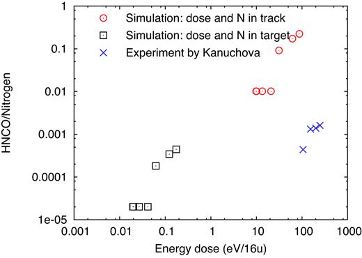
Abundance of HNCO molecules formed by irradiation relative to N atoms originally present in the specimen as a function of the energy dose delivered in the target. Experimental data from Kaňuchová et al. (×). Simulation data either refer to the track volume (⊙) or the entire simulation volume (|$\Box$|).
Lv et al. (2014a) irradiated an ice mixture consisting of |${\rm NH_3}$|, |${\rm H_2O}$|, and |${\rm CO_2}$| with 144 keV S ions. Besides the decreasing column density of the original molecules, the production of |${\rm N_2O}$|, |${\rm OCN}$|, and carbon monoxide was observed, and in addition ammonium in the form of ammonium formate, [|${\rm HCOO^-}$|][|${\rm NH_4{^+}}$|], carbamic acid, |${\rm NH_2COOH}$|, and ammonium carbamate, [|${\rm NH_2COO^-}$|][|${\rm NH_4{^+}}$|]. Some of these species only appeared after annealing at 160 K. Products of sulfur were not seen in these experiments because of the low ion flux. These results are in qualitative agreement with our simulations, where |${\rm CO}$| is an abundant fragment and ammonium, |${\rm NH_4{^+}}$|, a frequent product at all ion energies, and also isocyanic acid, |${\rm CHNO}$|, and cyanide, |${\rm CN}$|, are produced at all ion energies above 2.3 keV.
Augé et al. (2016) perform MeV irradiation experiments on nitrogen-rich ices using swift heavy ions, such as 44 MeV Ni and 160 MeV Ar, which have similar effects as the S ions studied in this work. Their ices are based on mixtures of |${\rm N_2}$| and |${\rm CH_4}$|, which contain water as impurities. They observe the production of |${\rm NH_3}$|, |${\rm NH_4{^+}}$|, |${\rm CO}$|, |${\rm CO_2}$|, |${\rm HNCO}$|, |${\rm OCN^-}$|, |${\rm CN^-}$|, and |${\rm HCN}$|. This is in qualitative agreement with the simulation results using S ions close to the stopping power maximum, 20 MeV, see Table 2, where we observe the production of |${\rm CO}$| as the most frequent fragment, followed by |${\rm NH_4}$|, |${\rm HNCO}$|, and various isomers of |${\rm CNO}$|.
Muñoz Caro & Schutte (2003) performed experiments on ice mixtures which closely resemble those used by us; they employed mixtures of |${\rm H_2O}$|, |${\rm CO_2}$|, |${\rm NH_3}$|, and |${\rm CH_3OH}$|, as we do, and add |${\rm CO}$|. The latter species is however abundantly produced as a fragment in our simulations as well. Instead of ion irradiation, they process the ices by UV light; they report the observation of formaldehyde, ammonium (|${\rm NH_4}$|), carbon acids, and amides, which are comparable to the results of our study. In addition, they slowly warm up the ices to room temperature, in order to study the further chemical evolution. As a consequence, they observe a large contribution of refractory materials attributed to hexamethylenetetramine, |${\rm (CH_2)_6N_4}$|, ammonium salts of carboxylic acids, amides, and esters, as well as species related to polyoxymethylene, |${\rm (-CH_2O-)_n}$|. Similar experiments were later performed by Nuevo et al. (2008), who also found complex molecules – including amino acids – after heating to room temperature.
4.2 Estimation of total molecule production
In Section 3.1 above, we had shown that the number of products and dissociations in the simulation volume shows a linear dependence on the deposited energy, Edep, cf. Fig. 4. This holds true for ion energies above 13.5 keV; below this energy, due to the strong increase in nuclear energy deposition, slight deviations from linearity are observed.
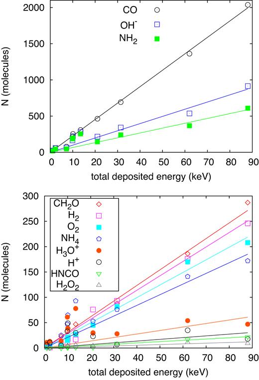
Number N of (a) CO, OH, and |${\rm NH_2}$| molecules and (b) less abundant product molecules generated as a function of the energy deposited by the ion in the simulation volume, Edep. Lines denote a proportionality, equation (6).
Production coefficients, ki, equation (6), numbers of molecules generated, Ni, and corresponding column densities, ρi, of abundant products i generated by a 20 MeV S projectile throughout its trajectory.
| Species | |${\rm CH_2O}$| | |${\rm CO}$| | |${\rm CHNO}$| | |${\rm NH_2}$| | |${\rm NH_4}$| | |${\rm OH}$| | |${\rm H_2}$| | |${\rm O_2}$| | |${\rm H^+}$| | |${\rm H_3O^+}$| | |${\rm H_2O_2}$| |
|---|---|---|---|---|---|---|---|---|---|---|---|
| ki (keV−1) | 3.1 ± 0.3 | 22.7 ± 0.4 | 0.25 ± 0.03 | 6.7 ± 0.4 | 2.1 ± 0.2 | 9.9 ± 0.4 | 2.8 ± 0.1 | 2.5 ± 0.2 | 0.34 ± 0.13 | 0.69 ± 0.13 | 0.14 ± 0.03 |
| Ni | 62 000 | 454 000 | 5000 | 134 000 | 42 000 | 198 000 | 56 000 | 50 000 | 6800 | 13 800 | 2800 |
| ρi (1015 cm−2) | 15.5 | 114 | 1.25 | 33.5 | 10.5 | 49.5 | 14 | 12.5 | 1.7 | 3.5 | 0.7 |
Deviations from the simple proportionality, equation (6), show up in the regime of dominant nuclear stopping, at energies around 13.5 keV; these will influence the end-of-range production yields, when the projectile is about to be stopped. These deviations do, however, only marginally influence the total production yield, equation (7), since for the major part of the trajectory, the ion is in the electronic-stopping regime, where the proportionality holds well. Note furthermore that deviations from proportionality appear to increase for the less abundant products; we assume that these are caused by fluctuations due to the small number of products monitored. Finally, some species – notably H and |${\rm H_3O}$| – show no increase with Edep; their number seems to saturate. We surmise that this is caused by the rapid reaction rate of H (and of |${\rm H_3O}$|, which is in equilibrium with it) which prevents stronger H concentrations from building up.
An approximate proportionality of the number of product molecules with ion energy has indeed been found in laboratory experiments such as by Vasconcelos et al. (2017) who irradiated ice samples with MeV ions; already earlier sputtering experiments showed an approximately linear increase of the radiolytic products with ion energy for irradiation with keV ions (Bar-Nun et al. 1985). Experiments also show, however, a saturation of some product species with fluence, see for instance Pilling et al. (2011). Analogously it might happen that a species concentration saturates within a single ion track, as we observe for H and |${\rm H_3O}$| in Fig. 23.
4.3 Influence of track radius
The model presented in this paper starts with a cylindrical track volume, which is energized by the swift projectile ion. While several restrictions of this assumption have been discussed in Section 2.2, the most important model parameter appears to be the track radius R. It has been fixed in our study to the value of R = 5 Å; in this section we shall study the dependence of the results on this parameter by using track radii of R = 10 and 20 Å. This will only be done for the highest energy case, 20 MeV, where the electronic energy deposition is largest. For these cases of increased track radius, we also slightly increased the lateral width of the simulation volume from 200 to 240 Å, such that the number of simulated atoms amounts to 1 376 448. These simulations were run only up to 13 ps, since then the number of products and fragments has already stabilized, as Fig. 5 and similar demonstrate.
The total number of products decreases from 5284 (R = 5 Å) over 4803 (R = 10 Å) to 3013 (R = 20 Å). Also the total number of dissociations decrease from 3672 via 3379 to 2130. These changes reflect the decreased initial track temperatures; as these decrease by a factor of 4 when the radius is doubled, the number of bond dissociations and reformations are correspondingly reduced. The decrease in products and fragments is only around 8–9 per cent when doubling the radius from R = 5 to 10 Å; this behaviour is analogous to that obtained previously for cosmic ray impact with ice grains (Mainitz et al. 2016) – with comparable stopping power of 100 eV/Å –, where it was shown that the broader track radius leads to only small (2 per cent) changes in the chemical transformation.
Clearly, upon further increase of the initial track radius, all bond dissociations and further reactions will become improbable as the temperature drops below the dissociation thresholds and the activation energies for reactions. This feature points at a weak aspect of the cylindrical track model used here; the model of an inhomogeneous track – with temperature decaying as 1/r2 with radial distance r from the ion trajectory (Waligorski et al. 1986) – might be more realistic in this respect. In addition, in reality, the electronic energy deposition occurs via discrete ionization events, which produce directly dissociated species and radicals available for further reactions in the vicinity of the ion trajectory; this feature is only approximately integrated in the thermal track model used in this paper.
Fig. 24 displays the mass spectra of the newly generated species for varied track radii, while Table 9 lists the products and their abundances. The products observed can be divided into several groups.
For several species – |${\rm CO}$|, |${\rm CHNO}$|, |${\rm CH_3O}$|, |${\rm CH_3N}$|, |${\rm CH_6O_2}$|, |${\rm C_2H_2}$|, |${\rm C_2H_2O}$|, |${\rm NH}$|, |${\rm NH_2}$|, |${\rm NH_4}$|, |${\rm OH}$|, |${\rm O_2H}$|, |${\rm HOH}\cdots{\rm OH}$| – the decreasing temperature with increasing track radius leads to a decline in abundance. This is the typical behaviour expected in particular for dissociation reactions.
A few species – |${\rm CHO}$| and |${\rm CH_3}$| – show the opposite increasing trend. Such radicals will indeed be consumed in follow-up reactions at high temperatures.
A third large group – |${\rm CN}$|, |${\rm CH_2N}$|, |${\rm CH_5O}$|, |${\rm C_2HO}$|, |${\rm C_2HO_2}$|, |${\rm NO}$|, |${\rm NHO}$|, |${\rm NHO_2}$|, |${\rm NH_2O}$|, |${\rm NH_2O_2}$|, |${\rm NH_3O}$|, |${\rm NH_3O_2}$|, |${\rm NH_4O}$|, |${\rm H}$|, |${\rm H_2}$|, |${\rm O}$|, |${\rm H_3O}$|, |${\rm O_2}$| and |${\rm H_2O_2}$| – shows highest abundance at intermediate temperatures (corresponding to a track radius of 10 Å). For these species, too high temperature might activate reactions consuming them, while the lowest temperature does not activate their formation.
Finally, in a few cases – formaldehyde, |${\rm CH_2O}$|, and methane, |${\rm CH_4}$|, – the smallest abundance is observed at the intermediate temperature. Here, a high initial temperature induces the reactions creating them, while at low temperatures follow-up reactions are inhibited.
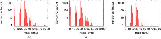
Simulated mass spectra of molecular products found for an ion energy of 20 MeV for several initial track radii: (a) 5 Å, cf. Fig. 6, (b) 10 Å, and (c) 20 Å.
Molecular products formed at an ion energy of 20 MeV for various track radii R. Only species, of which at least three specimens are produced in one of the simulations, are included.
| Sum formula | Mass (u) | R = 5 Å | R = 10 Å | R = 20 Å |
|---|---|---|---|---|
| |${\rm CO}$| | 28 | 2037 | 2005 | 1158 |
| |${\rm CN}$| | 26 | – | 3 | – |
| |${\rm CNO}$| | 42 | 3 | – | – |
| |${\rm CHO}$| | 29 | 3 | 6 | 13 |
| |${\rm CHO_2}$| | 45 | 4 | 4 | 5 |
| |${\rm CHN}$| | 27 | – | 3 | 1 |
| |${\rm CHNO}$| | 43 | 22 | 15 | 2 |
| |${\rm CH_2O}$| | 30 | 287 | 157 | 228 |
| |${\rm CH_2N}$| | 28 | 2 | 4 | 1 |
| |${\rm CH_2NO}$| | 44 | 4 | 5 | – |
| |${\rm CH_3}$| | 15 | 8 | 27 | 32 |
| |${\rm CH_3O}$| | 31 | 141 | 59 | 47 |
| |${\rm CH_3N}$| | 29 | 6 | 3 | 1 |
| |${\rm CH_4}$| | 16 | 13 | 9 | 13 |
| |${\rm CH_4N}$| | 30 | 3 | – | 1 |
| |${\rm CH_5O}$| | 33 | 6 | 18 | 14 |
| |${\rm CH_6O_2}$| | 50 | 3 | 1 | 1 |
| |${\rm C_2HO}$| | 41 | 4 | 6 | – |
| |${\rm C_2HO_2}$| | 57 | 2 | 5 | – |
| |${\rm C_2H_2}$| | 26 | 6 | 6 | – |
| |${\rm C_2H_2O}$| | 42 | 7 | 2 | 1 |
| |${\rm NO}$| | 30 | 147 | 175 | 21 |
| |${\rm NH}$| | 15 | 31 | 13 | 5 |
| |${\rm NHO}$| | 31 | 1 | 59 | 28 |
| |${\rm NHO_2}$| | 47 | 1 | 10 | – |
| |${\rm NH_2}$| | 16 | 610 | 391 | 316 |
| |${\rm NH_2O}$| | 32 | 9 | 27 | 16 |
| |${\rm NH_2O_2}$| | 48 | 1 | 3 | – |
| |${\rm NH_3O}$| | 33 | 35 | 120 | 93 |
| |${\rm NH_3O_2}$| | 49 | – | 5 | – |
| |${\rm NH_4}$| | 18 | 172 | 119 | 104 |
| |${\rm NH_4O}$| | 34 | 7 | 23 | 17 |
| |${\rm H}$| | 1 | 18 | 26 | 19 |
| |${\rm H_2}$| | 2 | 246 | 298 | 86 |
| |${\rm O}$| | 16 | 1 | 10 | 7 |
| |${\rm OH}$| | 17 | 915 | 642 | 510 |
| |${\rm H_3O}$| | 19 | 47 | 49 | 44 |
| |${\rm O_2}$| | 32 | 208 | 218 | 19 |
| |${\rm O_2H}$| | 33 | 8 | 8 | – |
| |${\rm H_2O_2}$| | 34 | 9 | 20 | 1 |
| |${\rm HOH}\cdots{\rm OH}$| | 35 | 15 | 7 | 6 |
| 2|${\rm H_2O}$| | 36 | 26 | 3 | 1 |
We conclude that the thermal track model used commonly in MD simulations – based on the assumption that a cylindrical volume around the ion trajectory is homogeneously filled with thermal atomic energy – is an approximation to the complex processes involving free electrons, ionization, and excitation processes. It requires a sufficiently small track radius R in order to be able to include the hot-chemistry reactions occurring in the track volume. Experimental data for track radii in ices are not available; this is in contrast to the situation in ceramics, where track radii may be inferred from measured molten (or amorphized) structures (Klaumünzer 2006).
5 CONCLUSIONS
We used MD simulation to study the effects of S ion impact on a cometary ice mixture. By using a REAX potential that is able to simulate bond breaking and reformation, we were able to keep track of the chemical processes that occur after impact. Electronic stopping is modelled in our approach by a thermal track model. We find that it is necessary to use a sufficiently small track radius in order to be able to include the hot-chemistry reactions occurring in the track volume. While we primarily aim at understanding the processes induced by a 20 MeV S ion, close to the stopping power maximum, we segment the ion trajectory to smaller pieces that fit into our computational box. Thus, we also obtain answers on how the ice responds to ion irradiation at lower energy, ranging down to 1 keV. Our scenario thus corresponds to an ice surface irradiated by sulfur ions in the magnetosphere of Jupiter; the various segments of the ion trajectory can be translated to different depths below the surface, where the induced reactions are studied.
We find that the numbers of dissociations and ensuing reactions scale approximately linearly with the deposited energy. Also, the most complex molecules are formed at the highest energy densities; this feature is in agreement with experiment (Rothard et al. 2017). Since thermal conductivity is low in the ices studied, temperatures may stay hot for an extended period of time close to the tracks, thus enabling these reactions. It may be concluded that the most complex reaction products are to be expected close to the ice surface; deeper below the surface, where the ion stopping power has decreased, the reactions will lead to less complex products.
The linear dependence of the number of product molecules on deposited energy also holds true for individual product species, at least if they are sufficiently abundant. We conclude from this finding that the number of product molecules is to first approximation proportional to the projectile ion energy. Secondary reactions of the product molecules and saturation effects within the ion track may change this simple picture.
A slight deviation from the linear increase of the number of reaction products with deposited energy is found in the energy window following the nuclear stopping maximum; this occurs at 13.5 keV in our case. It is related to the fact that at these low energies, a collision cascade is established in the target. The branched geometry of this cascade deviates from the simple linear track structure governing the electronic-stopping regime, and allows for more abundant reactions, and again for more complex product formation. This collision cascade regime will govern the final stopping process of the projectile close to its end point.
Several of the fragments and products we observe have been identified by radio astronomy in the interstellar medium, on comets and in experiments using interstellar ice analogues. As an example, formaldehyde – known as an important pre-product of sugar synthesis – and |${\rm H_2O_2}$| as an indicator of radiolysis are observed in the simulations to be formed all along the ion track.
Our simulations end after several 10 ps after ion impact, when we find that the reaction yields have reached saturation. However, thermal processes, which may occur in the real environment, may alter the chemistry again, and such processes have been described in the literature and analysed in laboratory experiments (Muñoz Caro & Schutte 2003; Nuevo et al. 2008). In addition, subsequent ion impacts in or nearby the irradiated regions may further change the reaction outcomes.
ACKNOWLEDGEMENTS
We acknowledge financial support by the Deutsche Forschungsgemeinschaft within project Ur 32/27-2. Simulations were performed at the High Performance Cluster Elwetritsch (Regionales Hochschulrechenzentrum, TU Kaiserslautern, Germany).
