


ABSTRACT
The evolution of galaxies is governed by equations with chaotic solutions: gravity and compressible (magneto-)hydrodynamics. While this microscale chaos and stochasticity has been well studied, it is poorly understood how it couples to macroscale properties examined in simulations of galaxy formation. In this paper, we use tiny perturbations introduced by floating-point round-off, random number generators, and seemingly trivial differences in algorithmic behaviour as seeds for chaotic behaviour. These can ultimately grow to produce non-trivial differences in star formation histories, circumgalactic medium properties, and the distribution of stellar mass. We examine the importance of stochasticity due to discreteness noise, variations in merger timings, and how self-regulation moderates the effects of this stochasticity. We show that chaotic variations in stellar mass can be suppressed through gas exhaustion, or be maintained at a roughly constant variance through stellar feedback. We also find that galaxy mergers are critical points from which large (as much as a factor of 2) variations can grow in global quantities such as the total stellar mass. These variations can grow and persist for Gyr before regressing towards the mean. These results show that detailed comparisons of simulations require serious consideration of the magnitude of effects compared to run-to-run chaotic variation, and may significantly complicate interpreting the impact of different physical models. Understanding the results of simulations require us to understand that the process of simulation is not a mapping of an infinitesimal point in configuration space to another, final infinitesimal point. Instead, simulations map a point in a space of possible initial conditions points to a volume of possible final states.
1 INTRODUCTION
Numerical simulations of galaxy formation seek to map a set of initial conditions (ICs) to a final state, using (often phenomenological) models of the physics involved. By comparing the evolution of identical ICs with models based on differing physical assumptions, we can learn how these assumptions impact the large-scale behaviour of the galaxy. We then hope to determine which of those assumptions are correct by comparing to empirical evidence provided by observational studies. This relies on a primary assumption: that all the differences between two simulated galaxies generated with different models can be explained by the different physical processes captured by these models. This assumption is incorrect.
It has been known for decades that collisionless N-body systems exhibit irreversible, chaotic behaviour (Miller 1964; Kandrup & Smith 1991). While this is important for tracking the individual orbits of planets in a Solar system (Laskar 1994) or stars within a cluster (Miller 1964), it has generally been regarded as unimportant to the global evolution of galaxy-scale properties. Although collisionless dynamics in galactic potentials feature chaotic orbits (Henon & Heiles 1964; Pfenniger 2009), this feature has not been considered particularly important to the overall assembly and star formation history of the galaxy as a whole. In this paper, we show that the chaotic nature of N-body systems, especially when coupled to collisional gas and subgrid models for star formation and stellar feedback, limits the ability to interpret simulation studies of galaxy formation and evolution. This chaotic behaviour cannot be overcome with more sophisticated algorithms or higher resolution: it is a fundamental feature of the physics governing galaxy formation.
Perhaps even more critical than N-body chaos is the stochastic, chaotic behaviour of both compressible hydrodynamic and magnetohydrodynamic (MHD) turbulence. It has long been known that the structure of the interstellar medium (ISM) is highly inhomogeneous (Larson 1981). With a Reynolds numbers of 105–107, the ISM should be spontaneously turbulent (Elmegreen & Scalo 2004), and thus produce naturally the inhomogeneities we see. As Ottino (1989) identifies, compressible turbulence shares the quasi-ergodic properties of classical dynamical chaos, but in a much higher dimensional space. Turbulent ISM overdensities can collapse to form stars (Larson 1981), which can then inject further energy into the turbulent fluid through stellar feedback. These features mean that different physical scales within the ISM are strongly coupled to one another, and that small-scale stochasticity can quickly ‘pump’ large-scale variations. Adding to this is the fact that the ISM is magnetized (Beck et al. 1996) and that magnetized turbulence can be driven spontaneously through MHD fluid instabilities (Cho & Lazarian 2003; Eyink, Lazarian & Vishniac 2011), the ISM has many routes through which its dynamics may become chaotic. The question of whether these internal chaotic dynamics impact large-scale, galaxy averaged properties has yet to be addressed.
Many studies have looked at the difference between hydrodynamical schemes (Frenk et al. 1999; Agertz et al. 2007; Vazza et al. 2011; Kim et al. 2016), models for star formation (Hopkins, Quataert & Murray 2011; Benincasa et al. 2016) or feedback (Thacker & Couchman 2000; Wurster & Thacker 2013; Keller, Wadsley & Couchman 2015), or combinations of these (Nagai, Kravtsov & Vikhlinin 2007; Scannapieco et al. 2012). In general, the consensus seems to be emerging that subresolution physics models (i.e. those models used for radiative cooling, star formation, feedback, etc.) are the primary source of variation between models of galaxy formation (Scannapieco et al. 2012; Stinson et al. 2013; Su et al. 2017b). Trajectories of individual resolution elements are almost never considered in these studies, for exactly the reasons above: they are well known to be chaotic, and understanding the causal chain that results in diverging trajectories is infeasible. Instead, we look at globally averaged properties: stellar masses, star formation rates (SFRs), density probability distribution functions (PDFs), etc. However, these properties are ultimately a consequence of the trajectories followed by the components of a simulated galaxy.
The effect of chaos on collisionless systems has been well studied. It has been demonstrated by Sellwood & Debattista (2009) that different random seeds used to generate ‘identical’ disc profiles can produce galaxies with a remarkably wide range of bar amplitudes and pattern speeds. In fact, this even applies for truly identical particle positions in their ICs, as they showed by reflecting a simple N-body disc galaxy about an axis, introducing different round-off errors from its twin, unreflected disc. They found that the Miller (1964) instability produces macroscopic differences in bar amplitude and pattern speed with a Lyapunov time 4 times shorter than the orbital period at 2.5Rd. For a galaxy like our own, that means nearly 280 e-foldings can take place in a Hubble time, more than enough time for perturbations to become non-linear. Benhaiem et al. (2018) have also recently observed similar macroscopic variations in the shape parameter of collisionless, virialized haloes.
Bar structures are important for bulge formation (Pfenniger & Norman 1990; Masters et al. 2011), active galactic nucleus (AGN) fuelling (Noguchi 1988; Laine et al. 2002), and may even help form dark matter cores (Weinberg & Katz 2002). This stochasticity may therefore be coupled to many other galaxy properties. On larger scales, Thiébaut et al. (2008) demonstrated that the chaotic behaviour is limited to non-linear structures on scales below |$3.5\, {\rm Mpc}\,\, h^{-1}$|. Within haloes, however, the positions and even the number of substructures can vary significantly due to small perturbations in the initial Gaussian random field from which they formed. Halo mass and spins are generally robust to small perturbations, but the direction of spin is not. A change in the substructure (and thus merger history), as well as the orientation of the disc relative to these structures, would likely have a non-negligible impact on the overall evolution of the galaxy within this halo. When coupled with hydrodynamics, star formation, and stellar feedback, these small perturbations may grow to significant differences in the evolution of ISM, the star formation history, and the distribution of metals.
The astrophysical discipline that has put the most thought into chaos and reproducibility (when it comes to the interpretation of simulation results and actually calculating Lyapunov coefficients) is likely that of the formation and evolution of planetary systems. An excellent, if somewhat unsettling, example of this are the studies that have found our own Solar system is dynamically unstable (Laskar 1994; Batygin & Laughlin 2008; Laskar & Gastineau 2009). As Batygin & Laughlin (2008) showed, the Lyapunov exponents for all of the terrestrial planets are all on the order of 10−7 yr−1, meaning that the planets will experience hundreds of Lyapunov times in the remaining lifespan of the Solar system. Disturbingly, Laskar & Gastineau (2009) showed that perturbing the position of Mercury by 0.38 mm(!) can put it on a collisional path with the Earth in one of 2501 different realizations of these perturbed systems. This chaos also manifests itself in simulations of planet formation, as Hoffmann et al. (2017) showed. They found that identical ICs, run with an identical code, could still produce vastly different Solar systems simply due to different floating-point round-off errors introduced by non-deterministic parallel reductions, amplified by chaotic N-body interactions, resulting in a different collisional history.
Recently, a pair of papers (Su et al. 2017a,b) have used the stochasticity of galaxy evolution to constrain the importance of different physical mechanisms. Su et al. (2017b) modified their feedback coupling scheme, ‘re-shuffling’ feedback energy and momentum, randomizing which neighbours of a star particle receive which fraction of the ejecta for a set of five runs. Su et al. (2017a) simply changed the random number seed used for two runs. Su et al. (2017b) found little variation in the final stellar mass for their |$1.2\times 10^{12}\, {\rm M}_{\odot }$| halo, with significant noise in the instantaneous SFR. Su et al. (2017a) find, for a |$8\times 10^9\, {\rm M}_{\odot }$| halo, a factor of ∼2 variation in stellar mass formed, as well as order-of-magnitude instantaneous variation in outflow and SFRs (though both of these values are quite noisy).
In this study, we examine the numerical sources of microscopic perturbations that can drive ‘identical’ simulations to produce macroscopically divergent results. We show that these perturbations can arise in any code (by, for example, changing the seed of a random number generator (RNGs) or simply through asynchronous mpi reductions) and can result in divergent star formation histories under certain conditions. Our results show that macroscopic differences in the stellar masses, stellar disc profiles, and circumgalactic medium (CGM) properties are common in identical simulations of cosmological galaxies, and can persist for a significant fraction of a Hubble time. These results also show that, under the influence of stellar feedback, chaotic variations can be pushed towards a variances much higher than expected by Poisson noise alone, independent of galaxy properties or even the details of feedback implementation.
2 NUMERICAL METHODS CAN SEED PERTURBATIONS
In general, simulations can introduce perturbations into ‘identical’ ICs through three sources: discretization of the ICs (Romeo, Horellou & Bergh 2003; Romeo et al. 2008; van den Bosch & Ogiya 2018), the use of RNGs in subresolution models, and floating-point round-off. This study will focus on perturbations generated by the last two, but the results are general to any source of small perturbations. These perturbations are especially important because they will arise in comparison studies that use identical ICs with different simulation models.
Variations are also clearly introduced by algorithmic differences. A change to the method of solving the hydrodynamic or N-body equations will of course lead to different (hopefully small) error terms, which like the perturbations introduced by the previous sources, may grow exponentially due to the formally chaotic behaviour of N-body systems. Algorithmic differences can also occur with identical codes run on different hardware, such as a running with a larger or smaller number of cores. Changing the number of cores that a code is run on will change how the domain is decomposed, and this can lead to differences both in the error terms and in the floating-point round-off behaviour. This means that the variations explored in this paper act as an unavoidable floor to the ability to both compare simulations run with different physics, simulation codes, or even to reproduce past simulations on different hardware. Reproducible codes do exist (Springel 2010), which produce bitwise identical results, but in these cases, these codes merely fix as constant the error terms introduced by floating-point round-off. These errors still exist, however, and still perturb the solutions. To explore the range of variation in possible outcomes, such codes require explicit perturbations in ICs (as is done in Genel et al. 2018) or in parameters (as is done in Su et al. 2017a,b). If any additional perturbation is applied, such as changing parameters or subgrid models, all codes will produce different round-off-level perturbations, uncorrelated with previous runs, and unrelated to the physical differences between the parameters or subgrid model. Reproducible codes are not more reliable predictors of physical outcomes, but are simply easier to debug.
2.1 Random number generators
Star formation is not the only process that RNGs are used to model. Many feedback models also rely on RNGs. The popular Springel & Hernquist (2003) multiphase model for galactic wind formation relies on an RNG both to select whether a particle is given a momentum kick, but also for selecting the direction of that momentum kick (as do the kinetic feedback models of Dalla Vecchia & Schaye 2008; Hopkins et al. 2011). Dalla Vecchia & Schaye (2012) derive a stochastic formulation for energy injection that ensures a constant post-feedback gas temperature, which gives a probability for a gas particle to receive feedback energy inversely proportional to this chosen temperature.
2.2 Floating-point arithmetic
Removing all RNG-based subgrid models from a simulation will not necessarily banish run-to-run variation. Arithmetic on floating-point numbers is non-associative: a + (b + c) is not necessarily equal to (a + b) + c (Coonen et al. 1979). While this may seem trivial, considering that double-precision round-off errors are typically on the order of one part in 1015, as long as the Lyapunov time for the system being evolved is sufficiently small, even these minuscule errors can be amplified to become macroscopic changes in the final state of the system. Not only does this mean that simply changing the order of operations in the source code of a simulation software can drastically change the output of that simulation code, it can also cause bitwise-identical compiled executables to produce different results in certain cases.
It has been well documented in the computer science literature that on parallel systems, reduction operations (such as summations) are non-deterministic (He & Ding 2001; Diethelm 2012). Variations in network congestion, cache space, and other subtle, unfortunately non-idealized physical processes involved in machines running parallel reductions will introduce floating-point errors due to a change in the order of associative operations. While work has been done to propose deterministic, reproducible algorithms for reduction operations (Balaji & Kimpe 2013), these algorithms are still in the experimental stages, and have not become the default for commonly used parallel protocols such as mpi or o penmp. These variations in round-off error are the source of perturbations used in Hoffmann et al. (2017), and as they show, they can ultimately cause significant variations in astrophysical simulations.
Even in the case of single-threaded applications, or applications where parallel reductions are avoided, different compiler optimization options can potentially introduce differences on the order of the floating-point round-off. While the C99 (and later) standard guarantees that all optimization flags up to -O3 will produce bitwise-identical floating-point operations, using the -Ofast or -ffast-math compiler optimizations with gcc will not produce bitwise-identical results when comparing to compilations made without those flags. The Intel c Compiler, icc enables equivalent features by default.
Even if all of these issues are avoided, most large-scale simulations of galaxy evolution rely on checkpointing: periodically writing out the state of the simulation so that in the event of a hardware failure or a runtime longer than allowed by a queuing system the simulation can be restarted. This process of writing out the contents of memory and then re-reading them again can introduce subtle changes in the order of operations of a simulation, and again introduce floating-point round-off errors that can lead to different ‘identical’ simulations diverging based on when or if they resumed from a checkpoint.
3 NUMERICAL METHODS
We study how small, numerical perturbations grow by running multiple realizations of the same IC on the same machine, with the same number of cores, using the same compiled binary of our simulation codes.
3.1 Initial conditions
3.1.1 MUGS2 cosmological galaxy
The cosmological zoom-in simulation used in this study is a member of the McMaster Unbiased Galaxy Sample 2 (MUGS2) (Keller, Wadsley & Couchman 2016). The MUGS2 ICs were initially described in Stinson et al. (2010). The zoom-in ICs were selected from a |$50h^{-1}\, {\rm Mpc}$| pure N-body cube, using a Wilkinson Microwave Anisotropy Probe 3 Λ cold dark matter cosmology, with |$H_0=73\, {\rm km\, s}^{-1}\, \, {\rm Mpc}^{-1}$|, ΩM = 0.24, Ωbary = 0.04, |$\Omega _\Lambda =0.76$|, and σ8 = 0.76. The MUGS2 simulations have a gas particle mass of |$2.2\times 10^{5}\, {\rm M}_{\odot }$|, and a gravitational softening length of |$312.5\, {\rm pc}\,$|. A floor is applied to the smoothed particle hydrodynamics (SPH) smoothing length, ensuring it is never below 1/4 this value. The star formation threshold used for this galaxy is |$9.3\,\,\rm {cm^{-3}}$|, as was used in previous studies (Stinson et al. 2013; Keller et al. 2015, 2016). The particular galaxy we have used here is g1536, a halo with a virial mass of |$6.5\times 10^{11}\, {\rm M}_{\odot }$|. In the fiducial MUGS2 run, g1536 forms |$1.9\times 10^{10}\, {\rm M}_{\odot }$| of stars by z = 0. This particular halo has been used in a number of studies beyond MUGS and MUGS2 (Calura et al. 2012; Obreja et al. 2013; Nickerson et al. 2013), including the MaGICC simulations (Stinson et al. 2013).
3.1.2 Isolated dwarf
We also ran a series of simulations using a modified version of the AGORA (Kim et al. 2014) isolated Milky Way (MW)-like Galaxy. The AGORA comparison project has produced a common set of ICs for both cosmological zoom-in simulations as well as isolated galaxies, and used these ICs to compare nine different simulation codes (Kim et al. 2016). The details of the IC and how it was created can be found in Kim et al. (2014). We modify the AGORA MW to match the ‘isolated dwarf’ case used in Keller et al. (2014) in order to increase the gas depletion time when simulated without feedback. As in Keller et al. (2014), we scaled down masses by a factor of 100, and lengths by 1001/3 as compared to the MW ICs, preserving physical densities while lowering the gas surface densities by a factor of ∼4.5. The gas particle mass for this dwarf IC is thus |$850\, {\rm M}_{\odot }$|, and the softening lengths are set to |$4.3\, {\rm pc}\,$|. The IC has a total gas mass of |$8.6\times 10^7\, {\rm M}_{\odot }$|, and a stellar mass of |$3.43\times 10^8\, {\rm M}_{\odot }$|. The disc has a scale length of |$740\, {\rm pc}\,$|, a gas fraction of 0.2, and a scale height of |$74\, {\rm pc}\,$|. It is embedded within a halo with |$M_{200} = 1.074\times 10^{10}\, {\rm M}_{\odot }$|, with corresponding concentration parameter c = 10 and spin parameter λ = 0.04. With this IC, we used a star formation density threshold of |$50\,\, \rm {cm^{-3}}$|.
3.2 Simulation codes
To show that the effects we study here are independent of subgrid physics, gravitational solver, or hydrodynamics methods, we use two different simulation codes along with a variety of feedback algorithms. The two codes we use, gasoline2 and ramses, are Lagrangian and Eulerian (respectively) astrophysical simulation codes frequently used in simulations of galaxy formation. Both gasoline2 and ramses were modified to ensure that all RNGs were seeded with the same value for each run (0 in this case).
3.2.1 GASOLINE2
gasoline2 (Wadsley, Keller & Quinn 2017) is a modern update to the gasoline (Wadsley, Stadel & Quinn 2004) parallel treesph (Katz, Weinberg & Hernquist 1996) simulation code. gasoline pairs a Barnes & Hut (1986) KD-Tree method for solving Poisson’s equation, along with the Lagrangian SPH (Gingold & Monaghan 1977) method for solving Euler’s equations. gasoline2 includes a number of updates that improve the performance and accuracy of the hydrodynamics method originally used in Gasoline. These features include a Saitoh & Makino (2009)-style time-step limiter, Wendland C2 and C4 smoothing kernels, an artificial diffusion term first described in Wadsley, Veeravalli & Couchman (2008), and a unique geometrically averaged density force (Wadsley et al. 2017). These improvements allow gasoline2 to accurately handle problems involving strong shocks, multiphase flows, and problems involving mixing. This effectively eliminates the problems seen in so-called traditional SPH methods (Ritchie & Thomas 2001; Agertz et al. 2007; Read, Hayfield & Agertz 2010). gasoline has been used for hundreds of studies of galaxy formation, and gasoline2 has been used by dozens of studies already.
3.2.2 RAMSES
ramses (Teyssier 2002) is an Eulerian, adaptive mesh refinement (AMR) N-body and hydrodynamical code. AMR allows for spatial adaptivity, with higher resolution in regions (in this study) of increased density (the so-called quasi-Lagrangian mode). ramses solves the compressible Euler equations by means of an unsplit second-order Monotone Upstream-centered Scheme for Conservation Laws Godunov method (van Leer 1979), with a Harten-Lax-van Leer-Contact (HLLC) Riemann Solver. Poisson’s equation is solved for gravity using a ‘one-way interface’ scheme (Jessop, Duncan & Chau 1994). ramses includes physics for radiative cooling, star formation, and stellar feedback, which we describe in section 3.3. Like gasoline, ramses has been used for hundreds of studies of cosmological structure and galaxy formation.
3.3 Subgrid physics
3.3.1 Star formation
Both codes also rely on a maximum temperature and minimum density threshold to select eligible star-forming gas cells/particles. We use a maximum temperature of 15000 K, and a density threshold dependent on the resolution of the different ICs we simulate. (see Section 3.1)
3.3.2 Blastwave feedback (gasoline2)
3.3.3 MaGICC feedback (gasoline2)
The MaGICC feedback model extends the (Stinson et al. 2006) blastwave model by including the effects of early stellar feedback from ultraviolet (UV) radiation. In addition to the basic blastwave model, which handles energy input from SNII, 10 per cent of the total UV flux from the stellar population contained within a star particle is deposited into the surrounding 32 neighbouring gas particles as thermal energy. This injects ∼2 times the energy deposited by SNII. Unlike with the SNII, these particles do not have their cooling disabled. This model is designed to mimic the formation of Hii regions and the destruction of star-forming clouds by the radiation from massive stars. This model has been used for the MaGICC simulations (Stinson et al. 2013 describe this model, and the simulations that are later used in MaGICC), as well as the large NIHAO suite of zoom-in simulations (Wang et al. 2015).
3.3.4 Superbubble Feedback (gasoline2)
3.3.5 Delayed cooling feedback (ramses)
4 NUMERICAL EXPERIMENTS
4.1 Does stochasticity depend on code or subgrid model?
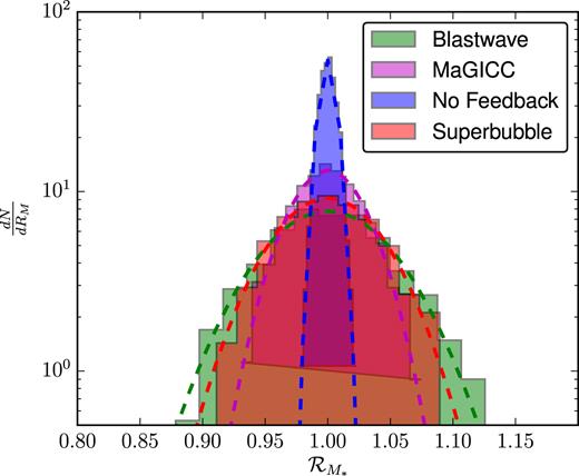
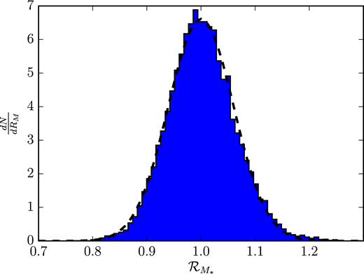
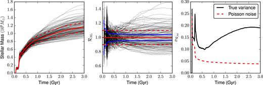
As one can see in Fig. 1, each pair of simulations shows variation on the order of |${\sim }10{{\ \rm per\ cent}}$| over the |$1\, {\rm Gyr}\,$| we evolve them for. The two cases with superbubble and MaGICC feedback appear to be closest to each other. We next resimulate the same IC, using superbubble feedback, 128 times. We thus calculate 128!/(2! · 126!) = 8192 different values of |$\mathcal {R}_{\mathcal {M}_{*}}$|, one for each unique pair of simulations from the set of 128. Again, all parameters and ICs are kept identical. As Fig. 2 shows, the variation in stellar mass from run to run is normally distributed, about |$\mathcal {R}_{\mathcal {M}_{*}} = 1$| (as we might expect), with |$\sigma _{\mathcal {R}_{\mathcal{M}}}=0.06$|. Thus, we can expect deviations of the order |$10{{\ \rm per\ cent}}$| from the mean stellar mass (at |$1\, {\rm Gyr}\,$|) in approximately |$10{{\ \rm per\ cent}}$| of runs.
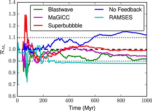
In this figure, we show the ratio of stellar masses formed in pairs of simulations run from identical ICs. Each curve shows the ratio of the stellar mass formed in an isolated dwarf with different feedback models (Blastwave, MaGICC, Superbubble, and No Feedback) and different simulation codes (gasoline2 for the former four curves, ramses for the cyan curve). If identical ICs and codes produced identical results, the ratio should be 1 (as shown by the black dashed curve). Dotted black lines show variations in stellar mass of |$\pm 10{{\ \rm per\ cent}}$|.
Histogram of the stellar mass ratios |$\mathcal {R}_{M_*}$| at |$t=3\, {\rm Gyr}\,$| for all pairs chosen from a set of 128 isolated dwarf simulations. Each of these galaxies began from identical ICs, and was evolved with identical code (gasoline2 using superbubble feedback). The solid histogram shows the distribution of mass ratios, with a fitted Gaussian shown by the black dashed curve. The mass ratios for these 8128 pairs are normally distributed, with σ = 0.06 about |$\mathcal {R}_{M_*} = 1$|.
4.2 Stochasticity without random numbers
The simulations shown in Fig. 1 all include RNG-based star formation models. As explained in Section 2.2, parallel floating-point reduction operations can result in non-deterministic behaviour. In gasoline2, only the hydrodynamics is implemented using parallel reductions for neighbour finding and force calculations.1 This means that a pure N-body run of the same ICs should be bitwise identical if run twice on the same number of threads. However, if the same simulation is run with hydrodynamic forces included, small seed perturbations in forces, on the order of 10−16, should be introduced in each force calculation. These seed perturbations may be amplified by the chaotic behaviour of turbulence and self-gravitation.
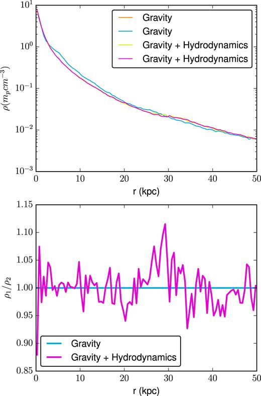
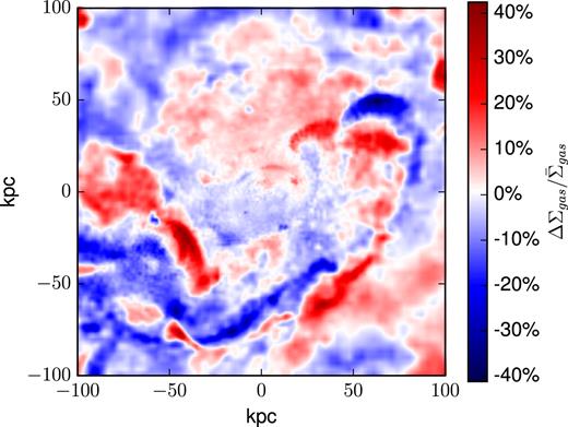
In Fig. 3, we show the results of a cosmological simulation run without star formation or feedback, once with gravity alone, and once with gravity and adiabatic hydrodynamics. This galaxy was evolved in each case to half the age of the universe, z ∼ 0.8. As is clear, the pure N-body case produces exactly the same density profile for the largest halo in the simulation, while the case with hydrodynamics shows noise in the density profile. The median absolute deviation (MAD) in the density ratios ρi, 1/ρi, 2 for all particles in the runs with hydrodynamics is 0.26 (we use the MAD here because of the long tail of large densities, which renders less robust statistics inaccurate). If one examines the differences in the gas distribution in these two adiabatic simulations, as Fig. 4 shows, deviations up to |$\gt 5\, {\rm M}_{\odot } \, {\rm pc}\, ^{-2}$|, or |$\pm 40{{\ \rm per\ cent}}$| can be seen in the column density of the halo. The MAD of the pixels in this 5002 column density map is 5 per cent, or |$0.17\, {\rm M}_{\odot }\, {\rm pc}\, ^2$|. The paired, offset structures that are visible in the column density difference show one of the major ways these perturbations grow in a cosmological simulation: small-scale chaos saturates to change the timings of merger and inflow events. Naturally, a change in the distribution and densities of gas within a galaxy will result in different star formation activity, the formation of different morphological structure, and may even change effectiveness of feedback by altering the density of the ISM surrounding the sites of star formation.
Without RNGs or parallel mpi reductions, as is the case when running gasoline2 without hydrodynamics or star formation, identical ICs (run with the same number of processes) can produce bitwise identical outputs. Here we show our cosmological halo’s density profile for two pairs of simulations, one run using gravity and hydrodynamics, and the other run using only gravity. The small perturbations between each run can be seen clearly in the bottom panel, where the gravity only case shows no difference run-to-run, while the case which includes hydrodynamics shows variations on the order of |$10{{\ \rm per\ cent}}$| from run to run.
Here, we show the difference in the column density of two pairs of cosmologically evolved haloes at z = 0.82. Each of these four simulations are evolved from the same ICs, with identical code. For one pair, gravity alone is used to evolve the IC, while the other uses gravity and SPH hydrodynamics. In gasoline2, gravity calculations do not use parallel mpi reductions, while SPH calculations do. These reductions introduce round-off-scale variations between the two runs with hydrodynamics, resulting in noticeable differences in the column density map.
4.3 Stochasticity in different dwarf systems
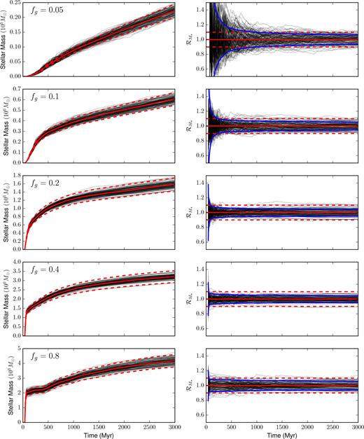
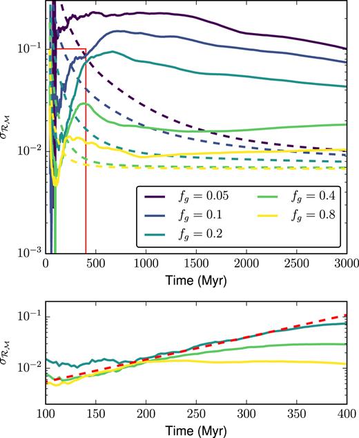
In Fig. 5, we show the result of simulating our dwarf with various gas surface densities, once again resimulating each IC 128 times. We use the superbubble feedback model for these simulations. By varying the disc gas fraction from fg = 0.05 up to 0.8 (the original IC has fg = 0.2), while keeping the total disc mass constant, we are able to vary the overall SFR and gas depletion times. As can be seen from the left-hand panels, the galaxies at high gas fractions experience a strong initial burst of star formation at |${\sim } 50\, {\rm Myr}\,$|, and continue to form stars more slowly for the remaining |$3\, {\rm Gyr}\,$| of their evolution. Despite the wide difference in the total number of stars formed across this range of gas fractions, the variation in each of the five cases is typically of the order of the shot noise, as seen in Fig. 6. As that figure shows, there is a large variation introduced by the initial burst of star formation, which rapidly decreases as star formation continues. We here fit a Gaussian to the distribution of |$\mathcal {R}_{\mathcal {M}_{*}}$| values, and plot the evolution of the distribution’s standard deviation σ over time. Each of these cases has standard deviation fairly well approximated as simple shot noise with |$\sigma = 2N_*^{-1/2}$|, where N* is the total number of star particles in the simulation. Naturally, this implies that for these isolated, fairly quiescent systems, the magnitude of this variation is resolution dependent, and will converge towards zero at higher resolutions. Of course, once individual stars are resolved this variance will saturate out.
Even when varying the gas fraction fg of the disc in our 128 dwarf simulations by a factor of 16, we can see in the left-hand panels that stochastic inter-run variations rarely deviate by more than |$\pm 10{{\ \rm per\ cent}}$| (red dashed curves) from the mean stellar mass (solid red curve). In the right-hand panels, we can see that the variation from the mean |$\mathcal {R}_{\mathcal {M}_{*}}$| is fairly well bounded by |${\sim } 2/\sqrt{N_*}$| shot noise, where N* is the mean number of stars formed by all 128 dwarf galaxies (blue curves).
The deviation in stellar mass formed in each of our quiescent dwarves (solid curves), as can be seen here, is fairly well approximated by Poisson noise (dashed curves). Stellar feedback is acting here to self-regulate star formation, and thereby reduce variations.
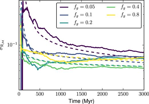
Unlike the case shown in Fig. 5, when the same dwarf is evolved without any form of feedback, deviations in the star formation history can grow without self-regulation. These deviations cannot grow without bound, however, as can be seen in the higher gas fraction cases, where the deviations fall well below |$10{{\ \rm per\ cent}}$|. These cases show more uniformity due to simple gas exhaustion: in every galaxy, virtually all of the gas has formed stars.
This figure shows the same evolution of stellar mass deviations shown in Fig. 6, but without any form of stellar feedback. As one can see, while the scatter in stellar masses decreases at higher surface densities, it still far exceeds what we would expect from pure Poisson noise (dashed curves). Notice also that the peak in |$\sigma _{\mathcal {R}_{\mathcal{M}}}$| occurs at earlier times as we go to higher surface densities: gas exhaustion occurs earlier and earlier as the SFR increases. The bottom panel is a zoom of the region shown in the red rectangle. The dashed red line shows an exponential with an e-folding time of |$100\, {\rm Myr}\,$|.
Results from the sets of 128 dwarf simulations. Each row shows the ICs and final results from 128 identical ICs run with and without feedback. Values in brackets are those from the simulations without feedback. Maximum values are filtered to only include values after |$100\, {\rm Myr}\,$| to remove the peak in |$\mathcal {R}_{\mathcal {M}_{*}}$| at the beginning of each run.
| fg | |$M_{\mathrm{ g},0}\,\, (10^6\, {\rm M}_{\odot })$| | tdep (no feedback) (Gyr) | SFE | Maximum |$\sigma _{\mathcal {R}_{\mathcal {M}_{*}}}$| | Final |$\sigma _{\mathcal {R}_{\mathcal {M}_{*}}}$| | Maximum |$\mathcal {R}_{\mathcal {M}_{*}}$| |
|---|---|---|---|---|---|---|
| 0.05 | 21.5 | 252.1 (9.191) | 1.0% (37%) | 0.38 (0.20) | 0.08 (0.10) | 2.49 (2.79) |
| 0.10 | 43 | 78.48 (6.365) | 1.4% (47%) | 0.16 (0.15) | 0.07 (0.07) | 1.41 (1.78) |
| 0.20 | 86 | 29.85 (2.166) | 1.8% (63%) | 0.07 (0.10) | 0.06 (0.04) | 1.28 (1.44) |
| 0.40 | 172 | 21.11 (0.735) | 1.9% (83%) | 0.06 (0.03) | 0.04 (0.02) | 1.23 (1.12) |
| 0.80 | 344 | 24.62 (0.420) | 1.2% (87%) | 0.08 (0.01) | 0.06 (0.01) | 1.35 (1.06) |
4.4 Stochasticity amplified by mergers
In more extreme star formation events, such as a merger-induced starburst, the run-to-run deviation can greatly exceed the |$2N_*^{-1/2}$| value seen in the previous runs. We built an IC by duplicating our fg = 0.1 isolated dwarf, and placing one copy |$50\, {\rm kpc}\,$| at |$45\deg$| from the galactic plane of its twin (with zero initial relative velocity), giving us a simple model of 1:1 major merger that occurs at |${\sim }200\, {\rm Myr}\,$|. When this merger occurs, as can be seen in Fig. 9, a rapid starburst is triggered. The variation in the timings of this starburst causes a brief spike in the stellar mass deviation to σ ∼ 0.25, along with a jump in the total stellar mass (pushing the shot noise down). As the starburst proceeds and eventually is extinguished by feedback, the stellar mass in the different runs begin to converge again, with the deviation eventually falling to σ = 0.1. The variations in the timings and locations of star formation during this merger is subsequently pumped up, returning the stellar mass deviation to σ ∼ 0.2. Some pairs of dwarf merger remnants reach final stellar masses after |$2\, {\rm Gyr}\,$| that differ by more than a factor of two (the pair consisting of the galaxy which forms ∼1.5 times the mean stellar mass and the galaxy which forms ∼0.7 times the mean stellar mass).
In a more violent system, such as this merger of two equal-mass dwarf galaxies, the starburst at |${\sim }200\, {\rm Myr}\,$| progresses differently in each system. Here, we show the stellar masses formed (leftmost panel), the deviation in stellar mass compared to the mean (middle panel) and the evolution of the variance (rightmost panel) for the sample of mergers. The variation in stellar mass formed in this event is rapidly suppressed by feedback and gas exhaustion. This variation leaves an indelible mark on each galaxy though, and after a few hundred Myr, the inter-run variation begins to grow as the star formation histories diverge from each other. As one can see in the leftmost panel, once the merger occurs, the inter-run variation in stellar mass greatly exceeds the shot noise.
4.5 Stochasticity in cosmological galaxy formation
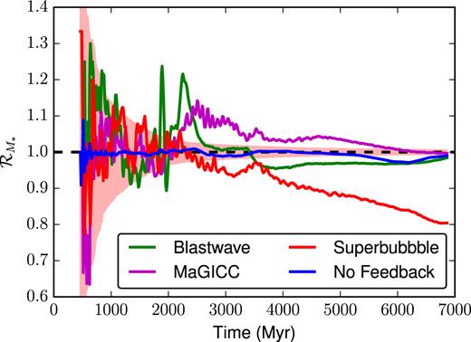
Cosmological galaxy evolution, especially in the early stages at high redshift, is characterized by many hierarchical merger events. Fig. 9 shows that numerical perturbations in mergers can precipitate long-lived deviations in the star formation histories that persist for Gyr. Fig. 10 shows that this effect is important in the more complex, realistic environment of a cosmological zoom-in simulation as well. We use gasoline2 to simulate four pairs of the MUGS2 galaxy g1536 to half the current age of the universe, z ∼ 0.9. Each pair is run using the different stellar feedback models that were earlier compared in Fig. 1. As can be seen, deviations of greater than |$10{{\ \rm per\ cent}}$| in the total stellar mass formed between the two simulations (which once again, use identical codes and ICs) occur and persist for Gyr. These deviations are much greater than the Poisson noise that our simple isolated dwarf galaxy exhibited in Fig. 6. The spikes seen in the blastwave runs just before and after |$2\, {\rm Gyr}\,$| are a result of timing variations in a gas-rich merger.
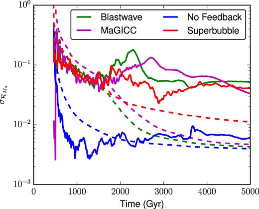
Here, we show the same plot of deviations in stellar mass between pairs as was shown in Fig. 1, but for a cosmological simulation of an MW-like galaxy. As the above figure shows, significant deviations in the stellar mass formed between two seemingly identical runs can grow and persist over Gyr time-scales. The shaded region shows the |$2/\sqrt{N_*}$| Poisson noise expected for the superbubble case. The dashed line at |$\mathcal {R}_{\mathcal {M}_{*}} = 1$| shows where the pair of runs form an equal number of stars.
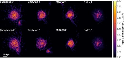
Even the qualitative appearance of these galaxies is noticeably different between runs. Fig. 11 shows the face-on gas column density for each of these cosmological galaxies. Each of the three pairs run with feedback show noticeable differences in the progress of a merger. The superbubble and blastwave cases each show one galaxy in the process of merging with a smaller companion, while the other has not yet begun to merge. One of the MaGICC discs has a clear tidal feature which is absent in its twin. Clearly, these differences in the distribution of gas will cause differences in the entire rest of the system.
Gas column density from the four cosmological simulations. Each column shows a pair of simulations run with identical code and parameters, for four different feedback models. As is clear, significant variation in the timing of a recent merger has occurred, with some cases (Blastwave 1 and Superbubble 2) having merged prior to their sibling runs.
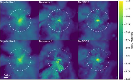
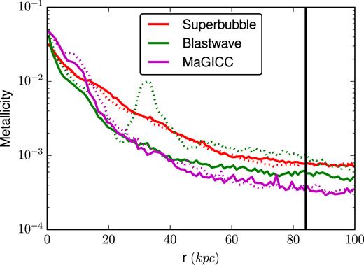
The global star formation history is not the only large-scale property where this stochasticity can be important. Stochastic differences manifest themselves quite prominently in the distribution of CGM metals, as is shown in the metal column densities of Fig. 12. As can be seen there, the merger timing offset in the two blastwave simulations causes a noticeable plume of metal-rich ejecta to be visible in one of the pairs, but absent in the other. If we take a profile of the radial metallicity, as in Fig. 13, we can see that this difference is significant. The two blastwave cases show a larger difference in the average metallicity from |$50\, {\rm kpc}\,$| out to the virial radius than any of the differences between any of the other cases using different feedback physics. When stochastic variation alone can produce changes in measured quantities this large, it is imperative that studies comparing different physical models take great care to show that the differences between simulations are actually the result of the change in physical model, and not mere stochastic variation. A naïve researcher could, given the results shown in Fig. 13, present completely contradictory results depending on which of the two ‘identical’ runs they happened to obtain for each of the simulations they compare. It is likely that the literature contains works that attempt to explain stochastic differences between runs as the result of important physical differences.
Column-averaged metallicity Σmetals/Σ for each of the three pairs of cosmological simulations that included feedback. Once again, there are clear variations in the amount and location of CGM metals within the virial radius (indicated by the dashed white circle). The large difference visible in the blastwave case is due to the delay offset of the merger visible in the previous figure. In case 2, the dwarf galaxy is polluting the CGM with metal-enriched outflows. Meanwhile, case 1 has already seen this dwarf merge with the central galaxy, and the CGM has become more well mixed.
Here, we show a mass-weighted radial profile of the metallicity in the haloes of each of our cosmological galaxies. Pairs using identical feedback physics are shown with identical colours. The metallicity of the CGM is clearly significantly affected by the inter-run stochasticity. In fact, the change in merger timing between the two Blastwave feedback runs produced a change on the order of the difference between the three different feedback models. An unlucky choice of runs for a comparison could come to exactly the opposite set of conclusions than another set of runs, at least where it comes to the flow of metals in the CGM. The black line indicates the virial radius at z = 0.82.
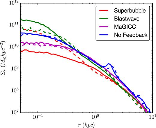
This magnitude of variation can also be seen in the profile of the stellar disc, as we show in Fig. 14. Once again, the variation between two twin simulations, in this case the superbubble runs, show a larger difference in the stellar surface density of the inner |$400\, {\rm pc}\,$| with each other than they do from the other simulations which use different feedback physics. All four cases show a cored central distribution of stars within the inner |$\, {\rm kpc}\,$|, which is likely due to the lack of resolved gravity with the softening length of |$320\, {\rm pc}\,$|. This flat central region shows a difference in stellar surface density between the two superbubble runs of roughly an order of magnitude.
In these cosmological simulations, the stellar disc surface density profile also exhibits strong stochastic effects. Here, one can see that within |${\sim }400\, {\rm pc}\,$|, the two Superbubble cases have nearly an order of magnitude difference in stellar surface density. Measurements of the stellar bulge in these two ‘identical’ systems would find wildly different bulge masses. A random choice of two pairs of simulations to compare the effects of different feedback models could, once again, come to opposite conclusions based purely on the stochastic inter-run variation.
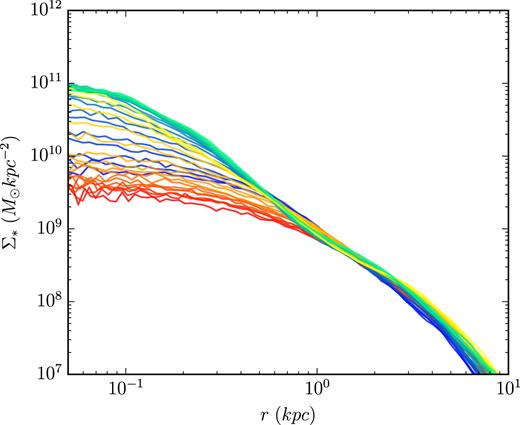
For quantities like these, where strong run-to-run variations are present, it is often the case that these are due to a fairly noisy, variable history. As we show in Fig. 15, the inner |$\, {\rm kpc}\,$| of the galaxy actually shows fluctuations of ∼1 dex over a period of |${\sim }1\, {\rm Gyr}\,$|. The two superbubble runs shown there, one coloured yellow to red for different times, each separated by |$110\, {\rm Myr}\,$|, the other coloured blue to green, vary from themselves over this time range by roughly as much as they vary from each other. The density of the central regions of the disc is clearly one of the properties that variations in the timing, kinematics, and gas-richness of mergers can strongly impact. This could be expected, as mergers are known to be a powerful mechanism for transporting angular momentum away from disc material, allowing it to form a central bulge (Toomre 1977). The sensitivity of a given quantity to the history of gas accretion and mergers on to a galaxy can often be used as a measure of the stochastic variations you may see when comparing two different runs. By examining a window of time before and after critical points like merger events, the uncertainty due to stochastic variation can be estimated.
The run-to-run differences seen in the stellar density profile are often of similar magnitude to the deviations over a period of |${\sim } 1\, {\rm Gyr}\,$| in individual simulations. Here, we show the stellar surface density profiles for five snapshots before and five snapshots after the profiles shown in Fig. 14. The snapshots are separated by |${\sim }100\, {\rm Myr}\,$|. We plot one of the superbubble runs using a blue–green gradient colourmap, and the other superbubble runs with a red–yellow gradient colourmap. As you can see, these two sets of simulations cover roughly the same range over this |$1\, {\rm Gyr}\,$| range. As much of the variation occurs from noise introduced in the timing of star formation events, mergers, and inflows, averaging over a period comparable to the dynamical time of the galaxy can often give an indication as to how much stochasticity one may see in a resimulation.
4.5.1 Statistics of stochasticity in cosmological environments
In order to better understand what is occurring in a fully cosmological context, where galaxies are neither isolated but instead experience tidal interactions, mergers, and continuous gas accretion, we have re-run the four sets of simulations from the previous section 32 times each, for a total of 128 cosmological zoom-in simulations, using four different models for feedback. We run these simulations to z ∼ 2 (|$5\, {\rm Gyr}\,$|).
A concern these results raise is whether comparisons between, for example, different feedback models may produce incorrect conclusions simply due to the effect size being smaller than the intrinsic stochastic variation in the quantity being measured for a galaxy. We show here in Fig. 16 that, for comparing feedback processes, stellar mass is a fairly robust indicator, with run-to-run scatter much less than the differences between different feedback models. Subtler effects, such as the changes introduced by varying diffusion models presented in Stinson et al. (2013) and Su et al. (2017b) do appear to produce changes in the stellar mass of the same order as the scatter shown here. In fact, the ICs simulated here are exactly the same as those used in Stinson et al. (2013), and the results we see here suggest that there is in fact no statistically significant difference between their ‘Fiducial’ case and their case with ‘Low Diffusion’.
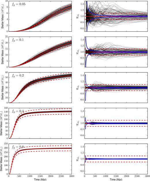
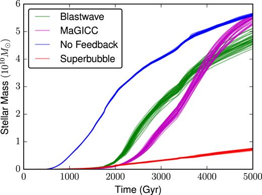
The stellar masses formed by |$5\, {\rm Gyr}\,$| for each of the 32 realizations of the same cosmologically formed galaxy, using the three different feedback models shown earlier (as well as a case without feedback). As is clear, the superbubble model forms significantly fewer stars than the two other feedback models. Despite the scatter between different realizations, the difference between realizations with different feedback models is still distinguishable.
Fig. 17 shows that the distribution of stellar masses formed with each of the four feedback models are roughly Gaussian, like our simple dwarf case shown in Fig. 2. It is clear, however, that the simulations run without feedback form a much narrower distribution of stellar masses, while the three cases with feedback all have similar scatter, with σ ∼ 0.05. The variance of this distribution is, for the three cases with feedback, constant to within a factor of a few, as is shown in Fig. 18. This is roughly an order of magnitude greater than the variance expected from Poisson noise alone, and the three different feedback models, despite producing quite different star formation histories, seem to all share a roughly indistinguishable variance in the total stellar mass formed over time. Without feedback, however, we can see that the variance is significantly lower, and in fact is comparable to the |$2/\sqrt{N_*}$| shot noise over the entire |$5\, {\rm Gyr}\,$| history of these simulations. Without feedback, these galaxies convert nearly their entire baryon budget into stars, suggesting that we are seeing low variance in this case simply due to gas exhaustion. The gas depletion times in these galaxies are so short that any run which lags behind the median has ample time to catch up, and those that rush ahead simply hit a wall of mass conservation: they cannot form more mass in stars than they have in baryonic mass.
Histogram of the stellar mass ratios |$\mathcal {R}_{M_*}$| at |$t=5\, {\rm Gyr}\,$| for all pairs chosen from the 32 cosmological galaxy simulations. The solid histogram shows the distribution of mass ratios, with a fitted Gaussian shown by the dashed curve. As is clear, the realizations that include feedback, regardless of which subgrid model is used, have a much broader distribution of stellar mass than those without.
The time evolution of the scatter between the 32 cosmological realizations for each feedback model. The 1σ scatter is shown with solid curves, while the |$2/\sqrt{N_*}$| Poisson noise is shown by the dashed curves. Despite having noticeably different star formation histories and final stellar masses, the three cases with feedback all have σ ∼ 0.05, roughly an order of magnitude larger than the scatter expected from Poisson noise alone. Meanwhile, the scatter in the case without feedback is reasonably well approximated by a the Poisson noise due to discrete star formation events.
5 DISCUSSION
5.1 Small effects are expensive to detect
The clearest result of these experiments is that identifying and distinguishing between subtle effects will require statistically meaningful samples and analysis to confidently detect. Countless studies have looked at changes in the star formation history, CGM/outflow properties, and disc morphology effected by different feedback models (e.g. Stinson et al. 2013; Smith, Sijacki & Shen 2017; Núñez et al. 2017), cooling schemes (e.g. Hu et al. 2016; Capelo et al. 2018), hydrodynamics methods (e.g. Hopkins 2015; Valentini et al. 2017; Su et al. 2017b), and star formation recipes (e.g. Su et al. 2017a). Each of these referenced papers presents at least some results comparable in magnitude to what we show here arises through stochastic variations alone. In order to be confident that these changes are physical, numerical studies must present some analysis of the stochastic variation intrinsic in their simulations.
Hoffmann et al. (2017) recommend eight identical runs for each case to give two samples per quartile of a uniform distribution. Our results suggest that variations are normally distributed, which unfortunately means a large number of cases are needed to sample the wings of the distribution. Despite that, for most simulations of galaxies evolved over more than a Gyr, short-term deviations can be used as an estimate for the uncertainty due to stochastic variations (e.g. see the peaks in the stellar mass ratio for each feedback-regulated galaxy in Fig. 10). In general, we find that feedback-regulated systems (at least in the mass scale we have tested here) rarely deviate from one another by more than |$50{{\ \rm per\ cent}}$| in total stellar mass formed. Detecting the effect of physical processes below this level will require either many (possibly dozens of) identical resimulations, or the simulation of large systems (i.e. cosmological volumes such as EAGLE, Crain et al. 2015, or Illustris ,Vogelsberger et al. 2014, or large samples of zooms such as NIHAO Wang et al. 2015, or E-MOSAICS, Pfeffer et al. 2018; Kruijssen et al. 2018). Large volumes and suites of zoom-in simulations provide a large enough sample of galaxies, already perturbed by their different ICs, to look at how different numerical models of physical processes manifest population-averaged changes. The variation within populations provided by these larger simulation projects can be used to compare to the magnitude of effects and evaluate their statistical significance. Stochasticity and chaos are not just the domain of dynamics: small-scale dynamical chaos couples to star formation and feedback, and can swamp smaller changes produced by the experimenter. Especially with systems involving mergers or bursty star formation, comparisons must take these uncertainties into account. While we do not recommend every simulator take the extreme route of running hundreds of copies of each simulation, a strategy similar to that advised by Hoffmann et al. (2017) is almost certainly necessary for comparing small (factor <2) variations in the quantities we have examined here. To the authors’ knowledge, only Su et al. (2017a,b) have resimulated identical ICs to gauge the uncertainty stochastic variations introduce in their simulations. Su et al. (2017b) use a set of five runs, with ‘re-shuffled’ feedback energy, while Su et al. (2017a) use a pair of simulations with different RNG seeds.
Measuring the uncertainty due to stochastic variation can be done fairly simply with resimulations. As Fig. 2 shows, stochastic variations in quantities like the stellar mass of a galaxy tend to be normally distributed. A simple way to add confidence intervals to simulations would be to select a reasonable point in the total lifetime of a galaxy (e.g. after the last major merger or the time at which the galaxy has assembled half of its mass), and resimulate that galaxy from thereon a number of times to generate a number of galaxy pairs. For example, in a cosmological simulation run to z = 0, 16 pairs of galaxies run for |$1\, {\rm Gyr}\,$| will yield 120 distinct pairs, and would require only slightly more computational time than re-running the original simulation to z = 0. A Gaussian fit to the ratios between these pairs can then be used to determine the variance (which can then be used to provide a 1/3/5σ confidence interval). Even if a code does not exhibit floating-point seeded stochastic differences, simply changing the number of threads used, the least significant bits of parameters/ICs, or the initial seed for the random-number generators can be used to introduce the seeds for chaotic variation. In order to quantify the amount of change that is due to the stochastic effects we examine here, you would still need to run multiple simulations, regardless of whether a code produces identical outputs when run without explicit perturbations. The direction of the random walk, and the distance from the median value for a given quantity is no better controlled in a reproducible code versus one which introduces small, floating-point level perturbations. Differences between simulations with alternative physical models which are smaller than this confidence interval require multiple simulations to demonstrate that an observed effect is not merely the result of stochastic variation.
5.2 Self-regulation and gas exhaustion are attractors
One of the interesting results we have found is that not only do stochastic variations exist for macroscopic quantities, but that the magnitude of these variations can vary in different systems. In those cases with depletion times much less than the |$3\, {\rm Gyr}\,$|, we evolved our dwarfs for (the cases without feedback and high gas surface densities) the final variation in stellar masses was minuscule (with a σ = 0.01 for the fg = 0.8 case). Here, the final stellar masses have an upper limit due to mass conservation: a galaxy cannot form more mass in stars than available in gas fuel. They have a lower limit due to the short depletion times relative to the time examined in the run: with an average depletion time of |$420\, {\rm Myr}\,$|, even if one galaxy’s star formation blazes ahead, the others will have plenty of time to catch up in stellar mass once the early star former exhausts its fuel. Without feedback, though, these galaxies wildly overproduce stars, converting up to 87 per cent of their initial gas mass to stars in the |$3\, {\rm Gyr}\,$| we run these simulations for. With more realistic, cosmologically modelled galaxies, the violent environment in which the galaxy forms drives nearly all galaxies towards star formation efficiencies of |${\sim }100{{\ \rm per\ cent}}$| when feedback is omitted, with gas depletion times |$\ll$|tHubble. Pushing the gas depletion time of a simulated galaxy to very low values will, as we have shown, reduce the final run-to-run variation in stellar mass, but at the cost of no longer actually modelling real galaxies. Observations reveal that most galaxies have molecular gas depletion times |$\gt \, {\rm Gyr}\,$| (Bigiel et al. 2011).
In the cases in which the gas depletion time is long, our simulations comparing galaxies with and without feedback show two clearly different outcomes. Without feedback, stellar masses can diverge chaotically, with a Lyapunov time of |$\lambda ^{-1}\sim 100\, {\rm Myr}\,$|, as shown by the fit in Fig. 8. These variations can persist for a significant fraction of a Hubble time. With feedback, the behaviour is somewhat more complex. For both cosmological galaxies and quiescent, isolated systems, the variance seems to be roughly constant, with σ ∼ 0.05. There appears to be no relation between the Poisson noise, depletion time, or even the feedback mechanism, and the width of the stellar mass distribution for multiple runs. Indeed, for our cosmological galaxies, which form many more stars (and thus have much lower Poisson noise), we can see that feedback can actually increase the variance compared to simulations run without feedback.
Stellar feedback acts to couple scales: star formation on small scales drives the injection of energy and momentum on much larger scales. As Figs 9 and 18 show, small-scale variations in the timing and progression of merger events can, through stellar feedback, couple to larger scales and drive variations in the star formation history of the galaxy that persist for |$\, {\rm Gyr}\,$| or more. However, these deviations cannot grow without bound. For our cosmological, MW-like galaxy, each of the three independent feedback models induced variance of σ ∼ 0.05 for the first |$5\, {\rm Gyr}\,$| of the galaxies evolution, roughly an order of magnitude above the Poisson noise. We see in Fig. 18 that a major merger event at |${\sim }1.5\, {\rm Gyr}\,$| drives up the scatter in each case, producing a similar effect as our idealized merger case shown in Fig. 9. Despite this, the variance never exceeds σ ∼ 0.2, despite sufficient gas supply to more than double the stellar mass in both the case of our idealized dwarf, and the cosmological galaxy (at least in the superbubble feedback case). Together, all these results suggest we have at least two ‘attractor’ solutions: a gas exhaustion/depletion equilibrium and a self-regulation equilibrium. In the case where depletion times are short, and feedback is inefficient, simple mass conservation prevents galaxies from exceeding the median mass, while the rapid conversion of stars to gas brings galaxies below this mass quickly towards it. When feedback is efficient, and thus depletion times are longer, the coupling of star formation to large-scale outflows, disc turbulence, etc. keeps the variance larger than expected from simple Poisson noise, but prevents it from growing without bound. A stochastic deviation that decreases the star formation will allow more gas to collapse and form stars (pushing the stellar mass up towards the attractor mass), while one that increases it will disrupt and heat more gas via feedback, thus pushing the stellar mass down towards this attractor solution. While each realization will evolve near this attractor solution, we can expect to find a not insignificant scatter around it.
5.3 Integrated quantities are less chaotic than instantaneous ones
In general, quantities that vary over shorter time-scales are more susceptible to small-scale chaos. For example, while the feedback-regulated dwarf galaxy with fg = 0.2 has a maximum |$\mathcal {R}_{\mathcal {M}_{*}}$| of only 1.28, its SFR, smoothed over |$20\,\,\, {\rm Myr}\,$|, shows maximum variations of more than a factor of 10 over the entire |$3\, {\rm Gyr}\,$| lifetime. This too is a manifestation of the self-regulation of star formation: when one galaxy begins to form stars at a rate above the mean, feedback ensures that its star formation rapidly drops, pushing it below the mean. The net result is that multiple runs show SFRs which oscillate incoherently about a mean SFR, with phase offsets introduced by small-scale stochastic variations.
Other quantities that can change on (relatively) short time-scales will also see large run-to-run variations. In particular, cosmological simulations can be sensitive to the timings of merger events. A comparison made between simulations that have recently experienced a major merger can be strongly impacted by slight offsets in the timing or trajectory of that merger, as can be seen in the CGM metallicity in Figs 12 and 13. Unfortunately, as our toy merger shows, it may take a significant amount of time for such differences to wash out. If a system experienced a major merger at relatively low redshift, a z = 0 comparison between two runs will likely be strongly affected by variations in the merger timings that occur between the two runs.
The variation in a single run over a short period of time can be used as a rough estimate as to whether run-to-run variation may be large enough to confuse a comparison. Looking at the instantaneous SFR in a short time window, for example, will be a poor measure to use in a comparison of bursty systems, as phase differences alone can produce large differences. As we showed in Fig. 15, while the stellar profile of our disc exhibits a factor of ∼10 variation in the peak surface density from run to run, this stochastic variation is comparable to the variation in any single run over |${\sim }1\, {\rm Gyr}\,$|.
5.4 Numerical considerations for reproducibility
Recent work in the stellar and planetary dynamics community has introduced some novel techniques for minimizing numerical seeds of chaotic and irreproducible behaviour in simulations of N-body systems (Boekholt & Portegies Zwart 2015; Rein & Tamayo 2017; Dehnen 2017; Rein & Tamayo 2018). As Laskar & Gastineau (2009) showed, errors on the order of a few hundred micrometres in the positions of a planet can lead to wildly divergent outcomes of a planetary system, and thus comparisons between different studies can be extremely difficult.
Rein & Tamayo (2017) presented modifications to the collisional N-body simulation package rebound that allows for machine independent, bitwise reproducible simulations from identical ICs. rebound is written in the C99 standard (see Section 2.2 for why this is important), and the authors have also implemented their own version of the pow() function. pow(), exp(), sin(), and cos() functions are all implemented in hardware-dependent ways, meaning different CPUs from different manufacturers, or even different CPU families from the same manufacturer may produce different round-off behaviour when these functions are used. Rein & Tamayo (2017) also implement a new binary output format that stores both the ICs, the version of rebound used to produce the simulation, as well as the Jacobi coordinates used for the Wisdom & Holman (1991) integrator, rather than inertial coordinates, to prevent round-off in recalculating these in a resimulation. These features allow bitwise reproduction of Solar system simulations.
The same authors presented a different solution to the problem of reproducibility in Rein & Tamayo (2018). This paper introduces a new integration scheme, janus, a high-order leap-frog integrator operating on 64-bit integers. As integer arithmetic is commutative, associative, and distributive, this means that janus is bitwise identical regardless of compilation or parallel communication details. As round-off is symmetric in time, this allows janus to be reversed in time from a final state, returning to the same ICs it began with. While this approach is well suited for N-body Solar system models, it is unlikely it would be applicable to galaxy simulations, which typically deal with much higher dynamic ranges, as well as additional physical processes unsuited for integer-arithmetic integration. And of course, as soon as non-adiabatic processes (radiative cooling, shocks, etc.) are included, reversibility becomes impossible. Beyond this, the value of ‘reproducibility’ is questionable when the physical system itself is formally chaotic.
Developing a reproducible code, whether from scratch or by adapting an existing code, can be a complex task. A large amount of software infrastructure would be required to support this: either algorithms would need to be rewritten to avoid reductions, or alternative implementations of the openmp and mpi reduction functions would need to be written.2 All subresolution models that rely on RNGs would require careful accounting that all RNGs are seeded identically, and that the RNG is identical across different machines and operating systems. This too may require a complete rewrite of the RNGs provided on most machines. Reproducibility across different machines would also require a reimplementation of basic transcendental functions normally implemented in hardware by the CPU: trigonometric, logarithmic, and exponential functions that are commonly used in simulation codes. Finally, if a code were to be reproducible for runs with different numbers of threads/processes, most domain decomposition and load balancing algorithms would require significant redesign. Many of these changes could potentially reduce the speed and efficiency of simulation codes. As we have shown here, this effort would simply aid in debugging, without actually reducing the uncertainty introduced by stochastic variations pumped by stellar feedback and N-body/hydrodynamic chaos.
5.5 The physical nature of stochasticity in galaxy formation
Even if we were to eliminate all uncertainty from our models and purge numerical artefacts from our codes, the fact would remain that infinitesimally small changes in ICs may still produce macroscopic changes in the final state of our galaxies. For studies in which one hopes to discover the effects of different models or parameters for subgrid physics, slightly perturbed ICs have the potential to yield quite different results.
Macroscopic chaotic behaviour makes interpreting the underlying causal relationship between models for galaxy evolution and the quantities one can measure difficult, regardless of ICs. Comparing the effects of different physical processes with identical ICs, even if simulated with some hypothetical, perfectly reproducible simulation code will still have sources for perturbations: those different physical processes. These will introduce small-scale, irrelevant changes (ones that can be amplified by the chaotic N-body and hydrodynamic equations), and large-scale, interpretable changes (the ones we hope to study). Is a decrease in bulge mass an effect of more efficient feedback (Keller et al. 2015), or a stochastic variation that has grown into a bar (Sellwood & Debattista 2009)? Is a more metal-rich CGM the effect of strong outflows (Shen, Wadsley & Stinson 2010), or a slight change in merger timing? Answering these sorts of questions with confidence requires some effort to be made in quantifying the magnitude of stochastic variations on the values being measured.
It is important to keep in mind that the numerical effects explored in this study are merely the seeds for chaotic behaviour: RNG seeds and floating-point round-off introduce only tiny, infinitesimal variations. The magnitude of the variations we see here are much greater than these initial seed perturbations, because the equations governing the evolution of galaxies have chaotic solutions. Both gravitational N-body interactions and hydrodynamic turbulence have well-known chaotic behaviour, and galaxies are self-gravitating, turbulent systems. The coupling of scales introduced by stellar feedback can, as we have seen, also act to amplify small-scale variations by converting them into larger scale injections of energy and momentum.
While this paper was under review, a related study was published by Genel et al. (2018). This work looks to quantify the same effects we examine here using a somewhat different strategy. Rather than looking at individual galaxies, Genel et al. (2018) use a series of cosmological volumes to look at population-scale differences. This allows them to run a smaller number of simulations (2–4 sets, depending on their choice of parameters), while still getting reasonable statistics on the magnitude of stochastic variation. They use the arepo (Springel 2010) hydrodynamics code, which has been carefully designed to avoid the numerical seed perturbations we have examined here. Instead, Genel et al. (2018) explicitly introduce perturbations in the positions of particles in the ICs on the order of floating-point round-off. On the scale of their |$50^3\, {\rm Mpc}$| simulation volume, this had the effect of adding to each particle a random position perturbation of |${\sim }10^{-7}\, {\rm pc}\,$|, roughly 5 solar radii. Despite having a completely different source for seed perturbations, Genel et al. (2018) found similar effects to those we present here. Critically, they found that without feedback, increasing resolution decreases the variation in global properties seen between their pairs of ‘shadow’ simulations, which is consistent with the variation being set by Poisson noise. However, with the IllustrisTNG feedback model (Pillepich et al. 2018), stochastic variations became independent of resolution. For one of the quantities measured, peak circular velocity, they found a distribution of variations with a standard deviation σ ∼ 0.05, remarkably similar to the distribution we find for stellar masses. Together, our study and Genel et al. (2018) point towards an interesting new phenomenon: the pumping of stochastic variation through stellar feedback. Coupling of large and small scales is a frequent feature of chaotic systems, and it appears that stellar feedback is another route by which this coupling can be established.
What these results require is a new way of understanding what numerical simulations are. Rather than mapping a point in the configuration space of possible ICs to a point in an equal-dimensional space of final states, numerical simulations sample a point within a volume of this configuration space, and map it to a point within a different volume. The size of this initial volume is constrained by the range of possible ICs that match a constraint we are concerned with: featuring a late major merger, forming a cluster-mass halo, etc. The size of the final volume is set by both the ICs and the physical processes involved in our models. Small perturbations, introduced either explicitly or implicitly through numerical effects, are a way to probe the size and shape of this volume.
6 CONCLUSIONS
We have shown that the small-scale dynamical chaos, seeded by numerical round-off and RNGs, can result in significant, long-lasting deviations in the star formation history and morphology of both isolated and cosmological galaxies. This fact has a number of implications:
Small differences between simulations generated with different physical or numerical models may actually be due to this large-scale stochasticity.
Attributing small (|$\lt\! 20{{\ \rm per\ cent}}$|) variations in averaged SFRs absolutely requires statistical evidence that this is not due to stochasticity. This means either running multiple simulations, or simulating large volumes which contain many objects. Other quantities are also quantitatively and qualitatively subject to stochastic variation.
Stochastic variation is important regardless of whether or not a code produces bitwise identical outputs. Insignificant changes to ICs or parameters can produce exactly the same effect, obscuring the causal relation between changes seen while comparing simulations.
Gas exhaustion and self-regulation by feedback can limit stochastic deviations, but often require |$\gt \! {\rm Gyr}\,$| of relatively unperturbed evolution to do so. Multiple mergers can push systems to diverge for most of the lifetime of the universe.
Stellar feedback efficiently couples different scales within the galaxy, and can result in an approximately constant level of variation |$(\sigma \sim 5{{\ \rm per\ cent}})$| well above what is expected from Poisson noise alone.
Rapidly varying quantities are more sensitive to stochastic variations than smoothed or integrated ones. Often the stochasticity in time is comparable to inter-run variation.
A single simulation samples a point in a volume of configuration space set by the ICs and physical model. Numerical non-determinism simply changes where in that volume the final state of the simulation ends.
We hope that readers do not interpret these results as a Jeremiad on the prospect of numerical simulation, but instead an exploration of a physical reality: galaxies are systems governed by evolution equations with Lyapunov times shorter than their lifetimes. This does not mean that numerical simulations are useless, or even that we must always run expensive suites of simulations in order to generate ensemble averages for all quantities we are interested in. Indeed, it is encouraging that our numerical models are now close enough to nature and each other that distinguishing between them is becoming non-trivial.
ACKNOWLEDGEMENTS
The analysis was performed using yt (http://yt-project.org, Turk et al. 2011) and pynbody (http://pynbody.github.io/, Pontzen et al. 2013). We thank Sam Geen and Bernhard Röttgers for useful conversations regarding this paper. We especially would like to thank Oscar Agertz and Romain Teyssier for providing the ramses AGORA ICs. The simulations were performed on the clusters hosted on scinet, part of ComputeCanada. We greatly appreciate the contributions of these computing allocations. We also thank NSERC for funding supporting this research. BWK and JMDK gratefully acknowledge funding from the European Research Council (ERC) under the European Union’s Horizon 2020 research and innovation programme via the ERC Starting Grant MUSTANG (grant agreement number 714907). BWK acknowledges funding in the form of a Postdoctoral Research Fellowship from the Alexander von Humboldt Stiftung. JMDK acknowledges funding from the German Research Foundation (DFG) in the form of an Emmy Noether Research Group (grant number KR4801/1-1).
Footnotes
More precisely, gasoline2 uses a wrapper library, the Machine-Dependent Layer, mdl (https://github.com/N-BodyShop/mdl), for communication. This library uses asynchronous mpi communication to build a neighbour list during neighbour finding. While the neighbour list is guaranteed to always contain the same members run to run, it does not guarantee that the neighbour list order is identical. This means that SPH force calculations and remote force summations will have run-to-run round-off-level differences due to the change in summation order.
This can be seen with gasoline2’s custom interaction-list based parallelism for gravity. The interaction lists used for gravity are inherited from pkdgrav, and forgoes the mpi reductions that are used for SPH sums in gasoline2. This is ultimately why the gravity-only gasoline2 runs are reproducible, while runs with hydrodynamics are not.
