


ABSTRACT
Exoplanet interior modelling usually makes the assumption that the elemental abundances of a planet are identical to those of its host star. Host stellar abundances are good proxies of planetary abundances, but only for refractory elements. This is particularly true for terrestrial planets, as evidenced by the relative differences in bulk chemical composition between the Sun and the Earth and other inner Solar system bodies. The elemental abundances of a planet host star must therefore be devolatilized in order to correctly represent the bulk chemical composition of its terrestrial planets. Furthermore, nickel and light elements make an important contribution alongside iron to the core of terrestrial planets. We therefore adopt an extended chemical network of the core, constrained by an Fe/Ni ratio of 18 ± 4 (by number). By applying these constraints to the Sun, our modelling reproduces the composition of the mantle and core, as well as the core mass fraction of the Earth. We also apply our modelling to four exoplanet host stars with precisely measured elemental abundances: Kepler-10, Kepler-20, Kepler-21, and Kepler-100. If these stars would also host terrestrial planets in their habitable zone, we find that such planets orbiting Kepler-21 would be the most Earth-like, while those orbiting Kepler-10 would be the least. To assess the similarity of a rocky exoplanet to the Earth in terms of interior composition and structure, high-precision host stellar abundances are critical. Our modelling implies that abundance uncertainties should be better than ∼0.04 dex for such an assessment to be made.
1 INTRODUCTION
We are at the cusp of the golden era of discovery and characterization of exoplanets. To date, more than 3800 exoplanets have been confirmed,1 via a wide range of observational techniques including transit photometry, radial velocity measurement, imaging, and microlensing (Winn & Fabrycky 2015). Continued improvements in observational and modelling techniques have led to more precise inference of planetary mass and radius (Weiss et al. 2016; Stassun et al. 2017b; Stassun, Collins & Gaudi 2017a). High-precision and homogeneous analyses of host stellar abundances are also increasingly available (e.g. Nissen & Schuster 2010; Adibekyan et al. 2012; Adibekyan et al. 2015; da Silva, Milone & Rocha-Pinto 2015; Brewer & Fischer 2016; Spina et al. 2016; Delgado Mena et al. 2017; Kos et al. 2018). At the same time, our knowledge of our own planet Earth and the Solar system has been enormously expanded with the efforts from the broad communities in geosciences, cosmochemistry, planet formation, and star formation (e.g. Ireland & Fegley 2000; McDonough 2014; Brasser et al. 2016a,b; Kwok 2016; Wang & Lineweaver 2016; Norris & Wood 2017; Wang, Lineweaver & Ireland 2018b). Together these have opened the door for detailed studies of chemical composition, interior structure, and habitability of rocky exoplanets.
Previous studies concerned with exoplanet interiors have generally assumed differentiated structures and molecular compositions to compute mass–radius relations (e.g. Seager et al. 2007; Valencia, Sasselov & O’Connell 2007; Howard et al. 2013; Zeng & Sasselov 2013; Dressing et al. 2015). It has been concluded that with only mass and radius measurements an exact interior composition cannot be inferred for an exoplanet because the problem is highly underconstrained or degenerate (Rogers & Seager 2010). With the increasing availability of elemental abundances of planet host stars, recent studies (Dorn et al. 2015; Santos et al. 2015) have discussed the reduction of degeneracies in constraining the interior composition and structure of rocky exoplanets by adding host stellar abundances as another principal constraint. Since then, an increasing number of updated models (with similar principal constraints) have been proposed (e.g. Unterborn, Dismukes & Panero 2016; Brugger et al. 2017; Dorn et al. 2017a; Dorn, Hinkel & Venturini 2017b; Unterborn et al. 2018), to improve the modelling of exoplanetary interiors.
However, a major cause of modelling inaccuracy inherent in the prevalent exoplanetary interior models (e.g. Santos et al. 2015; Brugger et al. 2017; Dorn et al. 2017a; Hinkel & Unterborn 2018; Unterborn et al. 2018) is that the elemental abundances of a rocky exoplanet are simplified to be identical to the elemental abundances of its host star. Host stellar abundances are good proxies of planetary abundances, but only for refractory elements.2 This is particularly true for terrestrial planets, as evidenced by the relative differences in the bulk composition between the Sun, Earth, and other inner Solar system bodies (Davis 2006; Carlson et al. 2014). This led Dorn et al. (2017b) to conclude that further studies of Solar system bodies are needed to improve our understanding of the correlation of relative bulk abundances between planets and host star and of the effect of such abundance correlations on exploring exoplanet interiors. Wang, Lineweaver & Ireland (2018a) has quantified the devolatilization (i.e. depletion of volatiles) in going from the solar nebula to the Earth. The elemental abundance differences between the Earth and the Sun for Si, Mg, Fe, and Ni are slight, but significant (a devolatilization factor of 10–20 per cent); those for O, S, and C are substantial and devolatilized by up to 3 orders of magnitude. The former differences, in combination with the substantially devolatilized O, will have a direct and non-trivial effect on the mantle and core composition; the latter differences will have profound impact on the atmospheric composition, including importantly the abundance of surface water, and therefore habitability in general.
An additional source of modelling inaccuracy in the prevalent studies of exoplanetary interiors is that elements lighter than Fe and Ni are rarely taken into account in the core composition. Light elements play a key role in compensating the 5–10 per cent density deficit of Earth’s core (Birch 1964; Hirose, Labrosse & Hernlund 2013; McDonough 2014; Wang et al. 2018b) (compared to pure iron at core pressures) and in differentiating the liquid outer core from the solid inner core. The importance of light elements in a terrestrial exoplanet’s core cannot be ignored, and their presence has direct consequences for estimates of core mass fraction and the melting temperature of an outer core (if it exists), and therefore the generation of exoplanetary magnetic fields.
With the goal of reducing the uncertainty in the estimates of interior composition and structure of terrestrial exoplanets, we present several important constraints and our analytical method in Section 2. Our modelling results are reported in Section 3, followed by the discussion in Section 4. We conclude in Section 5.
2 CONSTRAINTS AND ANALYSIS
2.1 Bulk elemental composition of a terrestrial planet
As mentioned earlier, elemental abundances between a terrestrial planet and its host star are not identical, especially for non-refractory or volatile elements. We argue that the elemental abundances of the host star of a terrestrial planet should be devolatilized in order to infer the planetary bulk composition. Wang et al. (2018a) has established a devolatilization fiducial model (see Fig. 1) by quantifying the compositional differences between the proto-Sun and the bulk Earth as a function of elemental condensation temperatures. This work is built upon the premise that devolatilization in a nebula may be universal and the Sun-to-Earth volatility trend (devolatilization pattern) of Wang et al. (2018a) is applicable to infer the bulk composition of terrestrial exoplanets, particularly those within circumstellar habitable zones. Some caveats and limitations of this assumption are discussed in the following paragraph (see Section 4.3 for more details).
![Devolatilization patterns from stellar nebulae to terrestrial exoplanets, which are drawn from the Sun-to-Earth volatility trend (devolatilization pattern) of Wang et al. (2018a), including the best fit (the solid line in black) and its 1σ uncertainty (the wedge in grey), as well as the devolatilization factors indicated by the dashed arrows. Host stellar abundance is normalized to 1 in linear (or 0 in dex), shown as the solid horizontal line in brown. The x-axis is the elemental 50 per cent condensation temperature (TC) in logarithm from (Lodders 2003), except for TC(C) and TC(O), which are adopted from Wang et al. (2018a) (see text). The left-hand y-axis is in the logarithmic scale for the planet (‘p’)-to-star (‘*’) elemental abundance ratio, (X/Al)p/(X/Al)*, while the right-hand y-axis is labelled in dex for the corresponding [X/Al] (=log ((X/Al)p/(X/Al)*)). Only elements that are essential to control the mineralogy of a terrestrial planet are indicated on this plot and then employed in our subsequent analysis.](https://oup.silverchair-cdn.com/oup/backfile/Content_public/Journal/mnras/482/2/10.1093_mnras_sty2749/3/m_sty2749fig1.jpeg?Expires=1749986447&Signature=LETIohxUm6lszi-KVFbai2ikiMN7ZzE0wuI8kWavW~nYcHnjayW3~dWBc8iihYaUVedjYRCYF7b9zOp-Fj7J~xlqqXI7y7EcgmNDeZX58v1965lWCDgyTBRyZp8bde8zGY4WpcQynWSf1okgzAZSqQFIKlaYqtytHT3mnZR6VTUMUSAOjYQlXk0la5qkQbLrJWfNF~az1-2koI2VuWCUft5iZgig1BxVX0ny83-t5whFWoD-W9lhQIo4hs4jDbU48IIXhBoV01uoSxVl7oEgICXNrL7qxcDW9-6n6qfXRU4g2r2IHEqGBap8UoqsBgqKtJf~IKz6tNSFAcrfrybmkA__&Key-Pair-Id=APKAIE5G5CRDK6RD3PGA)
Devolatilization patterns from stellar nebulae to terrestrial exoplanets, which are drawn from the Sun-to-Earth volatility trend (devolatilization pattern) of Wang et al. (2018a), including the best fit (the solid line in black) and its 1σ uncertainty (the wedge in grey), as well as the devolatilization factors indicated by the dashed arrows. Host stellar abundance is normalized to 1 in linear (or 0 in dex), shown as the solid horizontal line in brown. The x-axis is the elemental 50 per cent condensation temperature (TC) in logarithm from (Lodders 2003), except for TC(C) and TC(O), which are adopted from Wang et al. (2018a) (see text). The left-hand y-axis is in the logarithmic scale for the planet (‘p’)-to-star (‘*’) elemental abundance ratio, (X/Al)p/(X/Al)*, while the right-hand y-axis is labelled in dex for the corresponding [X/Al] (=log ((X/Al)p/(X/Al)*)). Only elements that are essential to control the mineralogy of a terrestrial planet are indicated on this plot and then employed in our subsequent analysis.
A variety of outcomes for the bulk composition of a rocky planet may result from composition-, location-, and time-scale-dependent differences in various (and sometimes contrary) fractionation processes, such as incomplete condensation (e.g. Grossman & Larimer 1974; Wasson & Chou 1974), partial evaporation (e.g. Anders 1964; Alexander, Boss & Carlson 2001; Braukmüller et al. 2018), accretionary collision (e.g. O’Neill & Palme 2008; Visscher & Fegley 2013; Hin et al. 2017), and giant impact in conjunction with magmatic solidification (e.g. Chen et al. 2013; Norris & Wood 2017; Dhaliwal, Day & Moynier 2018). The compositional differences of Earth, Mars, and Venus should be a measure of these variations within our own Solar system, but the extent to which the bulk compositions of Venus and Mars are different from the Earth is still debated in both the geochemical/cosmochemical community (e.g. Morgan & Anders 1980; Wanke & Dreibus 1988; Taylor 2013; Wang et al. 2018b) and the planet formation community (e.g. Kaib & Cowan 2015; Fitoussi, Bourdon & Wang 2016; Brasser et al. 2017; Brasser, Dauphas & Mojzsis 2018). We also note that the bulk compositions of Venus and Mars are not well determined yet and thus reliable quantitative analysis of bulk compositional differences between them and the Earth is difficult. We have been conservative to preclude the application of this algorithm to Mercury-orbit-like planets (e.g. warm super-Earths), as such planets may be more devolatilized than predicted due to plausibly more intensive stellar irradiation and bombardment histories. In spite of the complexity of planet formation, an essential step to improve the study of exoplanetary chemistry is to take into account devolatilization, with the best constrainable trend from the Sun to the Earth.
In Fig. 1, we plot 10 major elements (C, S, O, Na, Si, Fe, Mg, Ni, Ca, and Al) that are essential for estimating the mineralogy of a terrestrial planet and place these on the best-fitting devolatilization pattern of Wang et al. (2018a). These 10 elements account for more than 99 per cent of the total mass of Earth (McDonough 2014; Wang et al. 2018b). Conservative estimates of these elemental abundances and the mineralogy of rocky planets at varied orbital distances are presented in Section 3.3. It should be noted that these points are not observational ‘data’ but indications of the model-based devolatilization scales (i.e. planet-to-host abundance ratios) of these elements versus condensation temperatures (TC). These devolatilization scales are also numbered in the second and third columns of Table 1, in per cent (linear) and in dex (logarithmic), respectively. The normalization-reference element is Al, the most refractory major element. Normalizing to other refractory elements (e.g. Ca) will not affect the analysis or results, since this normalization will not change the relative abundance ratio of other elements to oxygen that is the key to determining the redox state of a planet. It is worth noting that the TC in Fig. 1 refers to 50 per cent condensation temperatures of Lodders (2003), except for C and O. As discussed in Wang et al. (2018a), an effective condensation temperature of C and O under the assumption of non-equilibrium multi-phase condensation is a better indication of the volatility of the two elements, than 50 per cent condensation temperature of them under the assumption of equilibrium single-phase condensation in Lodders (2003). We use their best estimates of the effective TC for C and O: 305 and 875 K, respectively.
Predicted bulk elemental composition [X/Al]a of potential habitable-zone terrestrial exoplanets as devolatilized from their host stellar abundances.b.
| Xc | FD (%)d | FD (dex)d | Kepler 10 (L16) | Kepler 10 (S15)e | Kepler 20 | Kepler 21f | Kepler 100 |
|---|---|---|---|---|---|---|---|
| C | 99.6 ± 0.1 | 2.42 ± 0.09 | −2.42 ± 0.09 | −2.29 ± 0.10 | −2.48 ± 0.10 | −2.38 ± 0.10 | −2.47 ± 0.12 |
| S | 93.4 ± 0.6 | 1.18 ± 0.04 | −1.20 ± 0.04 | – | – | −1.25 ± 0.06 | −1.23 ± 0.07 |
| O | 82 ± 1 | 0.74 ± 0.02 | −0.67 ± 0.03 | −0.39 ± 0.08 | −0.86 ± 0.08 | −0.73 ± 0.07 | −0.71 ± 0.10 |
| Na | 75 ± 1 | 0.60 ± 0.02 | −0.72 ± 0.02 | – | −0.65 ± 0.04 | −0.62 ± 0.05 | −0.57 ± 0.04 |
| Si | 20 ± 3 | 0.10 ± 0.02 | −0.17 ± 0.02 | −0.02 ± 0.03 | −0.14 ± 0.03 | −0.09 ± 0.03 | −0.13 ± 0.04 |
| Fe | 14 ± 3 | 0.07 ± 0.02 | −0.20 ± 0.02 | −0.07 ± 0.03 | −0.09 ± 0.06 | −0.09 ± 0.07 | −0.17 ± 0.08 |
| Mg | 14 ± 3 | 0.07 ± 0.02 | −0.10 ± 0.02 | 0.09 ± 0.06 | −0.05 ± 0.04 | −0.07 ± 0.04 | −0.10 ± 0.05 |
| Ni | 10 ± 4 | 0.05 ± 0.02 | −0.20 ± 0.02 | – | −0.07 ± 0.03 | −0.12 ± 0.03 | −0.11 ± 0.03 |
| Ca | 0 | 0 | −0.05 ± 0.01 | – | 0.00 ± 0.04 | 0.00 ± 0.04 | −0.06 ± 0.05 |
| Al | 0 | 0 | 0.00 ± 0.01 | – | 0.00 ± 0.02 | – | 0.00 ± 0.03 |
Notes.a[X/Al] = log [(X/Al)planet/(X/Al)Sun], where (X/Al) is the abundance ratio (by number in linear) of an element X to Al, and solar abundance refers to Asplund et al. (2009). Normalizing to a refractory element other than Al does not change our results. Following Wang et al. (2018a), we choose Al as the normalization element since it is the most refractory major element.
bSources of host stellar abundances: Kepler 10: L16- (Column 2 of table 2 of Liu et al. 2016); S15- (Row 2 of table A.1 and Row 2 of table A.2 in Santos et al. 2015). Kepler 20, Kepler 21, and Kepler 100: table 3 of Schuler et al. (2015).
cElements (X) are listed in order of decreasing devolatilization factor.
dFD: Devolatilization factor, which refers to Fig. 1. F(D) (%) of each element is derived by 1 − (X/Al)planet/(X/Al)Sun, where (X/Al)planet/(X/Al)Sun can be read from the left-hand y-axis according to the devolatilization pattern. The corresponding F(D) (dex) is directly opposite to [X/Al] { = log [(X/Al)planet/(X/Al)Sun)]}, which can be read from the right-hand y-axis according to the devolatilization pattern.
eThe elemental abundances of Kepler-10 (S15) planets are normalized to Fe abundance in the host star, as no available Al abundance for Kepler-10 is reported in Santos et al. (2015). This normalization difference will not change the subsequent analyses of key elemental ratios including Mg/Si, Fe/Si, and C/O.
fThe elemental abundances of Kepler-21 planets are normalized to Ca abundance in the host star, as no available Al abundance for Kepler 21 is documented in Schuler et al. (2015).
2.2 Chemical network of the mantle of a terrestrial planet
In this study, the mantle of a terrestrial planet is limited to silicate mineralogy. This limitation is appropriate for two reasons: (i) our devolatilization algorithm that is established for the Sun to a silicate-mantle terrestrial planet is unlikely to be applicable for a planetary system with C/O ratio larger than 0.8 (and thus forming carbide planets – see Bond, O’Brien & Lauretta 2010); (ii) more recent studies (e.g. Fortney 2012; Nissen 2013; Teske et al. 2014; Brewer & Fischer 2016) have suggested that prior studies (e.g. Bond et al. 2010; Delgado Mena et al. 2010; Petigura & Marcy 2011) overestimated C/O ratios, namely carbide planets may not be as abundant as previously thought.
We assume that the composition of silicate mantle varies within the chemical system of SiO2–CaO–Na2O–MgO–Al2O3–FeO–NiO–SO3. And it is similar to the NCFMAS (Na2O–CaO–FeO–MgO–Al2O3–SiO2) mantle model adopted in Dorn et al. (2015), but the oxides are reordered in the oxidation sequence (or ease of oxidation) (Johnson & Warr 1999). NiO and SO3 are also added into the system. Due to the strong affinity of Ni with Fe, NiO is always expected if FeO is present in the mantle. SO3 can combine with other oxides to form sulphate compounds (e.g. CaSO4), which are important minerals in the silicate mantle (though not as abundant as silicate compounds). The additions of NiO and SO3 will also make estimates of the partition of Ni and S into the core more accurate (see Section 2.3). Sulphide minerals (except for FeS) are the major host of chalcophile (sulphur-loving) elements, but they are not taken into account in our mantle system since the abundances of all chalcophile elements (e.g. Cu, Zn, and Ag) are negligible in comparison with the abundances of the major rock-forming elements considered here.
With regard to a planet’s mantle temperature (T), pressure (P), and oxygen fugacity (fO2, quantifying the oxidation potential of a system), the mineral host of carbon can be either oxidized carbonate species (denoted as C4 + or CO2 in an oxidized form) (Panero & Kabbes 2008; Boulard et al. 2011) or the reduced native element (e.g. graphite/diamond) (Walter et al. 2008; Dasgupta & Hirschmann 2010). Oxidized carbon will be considered only when all major elements listed in the chemical network of the mantle have been oxidized, since carbon is experimentally shown to be oxidized later than Fe (presumably Ni as well) over the entire pressure and temperature ranges of Earth’s mantle (Unterborn et al. 2014). We also assume that if oxygen fugacity is extremely limited, metals like Ca, Na, Mg, and Al can be present natively in the reduced environment of the mantle, while Fe and Ni will be all partitioned into the core.
2.3 Chemical network of the core of a terrestrial planet
We assume that a terrestrial planet’s core consists of the Fe–Ni–S alloy. Nickel is added into the core’s constituents as it has a similar siderophile tendency as iron. Sulphur is a leading candidate for the principal light element in the core because it has a strong affinity for iron (Li & Fei 2014), and indeed evidence for large-scale sulphide fractionation during Earth’s mantle-core differentiation has been found (Savage et al. 2015). This does not preclude the existence of other light element candidates like silicon and oxygen in the core, but their fractionation between the mantle and the core is very uncertain without knowing the actual internal pressure and temperature of such a planet (Hirose et al. 2017). Therefore, in this study, we limit the light element in a terrestrial planet’s core to be sulphur only. Furthermore, sulphur is capable of reducing the core’s melting temperature, density, and surface tension (Li & Fei 2014), which may be important to the dynamo modelling of planetary magnetic fields in further studies.
It is important then to put constraints on the fractionation of these elements between the mantle and core. The cosmic ratio of Fe/Ni is 17.4 ± 0.5 (by mass) as drawn from a variety of chondrites in the Solar system (McDonough 2017). This value could vary from star to star, but the variance should be small based on the nucleosynthesis of the two elements in stars. Indeed, by analysing the Fe/Ni ratios of more than 4900 FGK-type stars within 150 pc of the Sun from Hypatia Catalog (Hinkel et al. 2014), we have found that the number ratio of Fe/Ni is 17.7 with 1σ uncertainty of ∼2.0 (see Fig. 2). Although their ratio in the planetary core might not be fixed, it will deviate little from the cosmic ratio considering their very similar refractory and siderophile features (McDonough, private communication). Indeed, a recent metal-silicate partitioning experiment has shown the ideality of the Fe/Ni ratio at conditions similar to Earth’s core (Huang & Badro 2018). To be conservative, a value of 18 ± 4 (by number) is adopted to constrain the Fe/Ni ratio in the core of a terrestrial planet. This adoption is appropriate for this study as the upper limit (22) of this value has covered the maximum value of Fe/Ni of our selected planet hosts. The lower limit (14) is ∼1.5σ lower than the Fe/Ni ratios of our selected cases, but it is a good assumption as Fe/Ni in the core of a terrestrial planet may go lower (not higher) than its value in the bulk planet (Ringwood 1986; Seifert, O’Neill & Brey 1988; McDonough & Sun 1995; Wang et al. 2018b).
![Distribution of [Fe/Ni] of more than 4900 FGK-type stars within 150 pc of the Sun. The values of [Fe/Ni] and [Fe/H] are relative to the Sun (Asplund et al. 2009), drawn from the Hypatia Catalog (Hinkel et al. 2014). A Gaussian fit to the distribution of [Fe/Ni] gives [Fe/Ni] = −0.033 ± 0.049 dex (relative to [Fe/Ni]$\odot$ = 1.28 dex). The corresponding value of Fe/Ni in linear is 17.7 (=10−0.033 + 1.28) with 1σ uncertainty of ∼2.0. A conservative value of 18 ± 4 is adopted to constrain the Fe/Ni ratio in the core of a terrestrial exoplanet (see the main text). The yellow point represents the Sun while the red filled pluses indicate our case stars.](https://oup.silverchair-cdn.com/oup/backfile/Content_public/Journal/mnras/482/2/10.1093_mnras_sty2749/3/m_sty2749fig2.jpeg?Expires=1749986447&Signature=KKzHzwH53-TTIBMbQO4qKEjhH9vwE7MrVq6~WyBcz8C3sWpfe7dBvedwvIUtMRtEHnC5HUrK0UDqiw6RIp2wKNlP0THw20AL8wj~V-SuHgDQfzSirmwgN0xhgUnCOna34lGFdOjhmQ7i~I0VM3M4n5JbFLQsbs33jE0~sLd0~lkRttzO2dYzVmS9~p1A~aio~GPYZ8aXQkwcniarmyyZ1c2w2s8ZvG-NIE509k-fA-ZDDA~sbw7sL7nU~O83yZKIeZQGAFOfSzMG80HH9xAIiDJRlGV3uRb~zXyZx7069XXZ8oK0eitCG5Cb6MeErW0Mzf-vEX8XjJvxup7RMXb8qg__&Key-Pair-Id=APKAIE5G5CRDK6RD3PGA)
Distribution of [Fe/Ni] of more than 4900 FGK-type stars within 150 pc of the Sun. The values of [Fe/Ni] and [Fe/H] are relative to the Sun (Asplund et al. 2009), drawn from the Hypatia Catalog (Hinkel et al. 2014). A Gaussian fit to the distribution of [Fe/Ni] gives [Fe/Ni] = −0.033 ± 0.049 dex (relative to [Fe/Ni]|$\odot$| = 1.28 dex). The corresponding value of Fe/Ni in linear is 17.7 (=10−0.033 + 1.28) with 1σ uncertainty of ∼2.0. A conservative value of 18 ± 4 is adopted to constrain the Fe/Ni ratio in the core of a terrestrial exoplanet (see the main text). The yellow point represents the Sun while the red filled pluses indicate our case stars.
Another constraint is the abundance range of Ni and S that may be present in the core. The upper limits of Ni and S in the core can be up to their abundances in the bulk planet, referring to the scenario of the Earth: |$\gt 90{{\ \rm per\ cent}}$| of Ni and |$\gt 95{{\ \rm per\ cent}}$| of S are in the Earth’s core (McDonough 2014; Wang et al. 2018b). The lower limits can be assumed as nil, such as in the extreme scenario that the oxygen fugacity is too high and all metals including Fe could be fully oxidized (then a planet with no core would result) (Elkins-Tanton & Seager 2008). See more details in Section 2.4 and Appendix A.
2.4 Analysis
Our sample of planet host stars includes Kepler-10 (K10), Kepler-20 (K20), Kepler-21 (K21), and Kepler-100 (K100), each of which has been confirmed to host at least one super-Earth (with 3–10 Earth masses), with high-precision host stellar abundances (available for almost all 10 elements indicated in Fig. 1 while for at least Mg, Si, Fe, and O). For K10, we have two sets of stellar elemental abundances: Santos et al. (2015) and Liu et al. (2016). For other selected cases, our stellar elemental abundances are from Schuler et al. (2015) (with a typical uncertainty of ≲0.04 dex). The selection of these case stars in this work does not exclude the applicability of our method to other planet hosts in a more extensive case study in the future.
Following the recommended constraint on planetary bulk composition in Section 2.1, we apply the devolatilization pattern of Wang et al. (2018a) to the elemental abundances of the planet hosts of our sample. This leads to the first-order estimates of bulk elemental composition of potential rocky exoplanets that could be within the habitable zone around these host stars (see Table 1). For brevity and convenience, we call such an exoplanet ‘exo-Earth’ (or ‘exoE’ when it is preceded by the name of its host star). However, this term means nothing about the similarity of such a planet to the Earth, except for the connotation that this planet is derived from its host star based on the equivalent devolatilization scale from the solar nebula to the Earth (the limitations of this assumption are discussed in Section 4.3). The uncertainties on the bulk compositions of these exo-Earths in Table 1 are propagated from the 1σ uncertainty of the devolatilization pattern of Wang et al. (2018a) and the uncertainties associated with the elemental abundances of the corresponding planet hosts.
We analyse the key elemental ratios (e.g. Mg/Si, Fe/Si, and C/O) that modulate the primary mineralogy of a terrestrial planet. Mg/Si influences the rock types of a silicate mantle. A higher Mg/Si indicates a more olivine-dominated mantle, otherwise a more pyroxene-dominated one. Pyroxene can accommodate more water than olivine, and pyroxenites have higher capacity to hold water. Fe/Si may approximate the zeroth-order core mass fraction of a planet, upon the oxidation state of the planet. C/O is critical to determine the oxygen fugacity and thus the oxidation state of a planet. The errors in these key elemental ratios are calculated using a Monte Carlo approach by drawing 2 × 10⁴ values of the estimated planetary bulk composition for each element following a Gaussian distribution around the uncertainties.
Based on the recommended chemical networks for the mantle and core of a terrestrial planet in Sections 2.2 and 2.3, the elemental fractionation between the mantle and the core is performed using the stoichiometric balance between the budget of oxygen atoms in the bulk planet and the abundances of oxides/compounds to be considered for the planet. The computational procedure is summarized in Fig. 3, while a detailed description can be found in Appendix A.
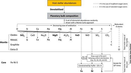
Computational procedure scheme of elemental fractionation between the mantle and the core of a terrestrial planet. The detailed descriptions of the procedure can be found in Appendix A.
As a verification for this set of computations, we apply this procedure to the proto-Sun (Wang et al. 2018a). The predicted planetary interior compositions of the model Earth in Table 2 are consistent (within uncertainties) with the independent estimates of the composition of the pyrolite silicate Earth (McDonough & Sun 1995), the composition of Earth’s core (McDonough 2014), as well as the seismologically constrained core mass fraction (Wang et al. 2018b).
Comparison of the estimates of the interior compositions of the model Earth (as devolatilized from the proto-Suna) with other independent estimates.
| Quantity | Model Earth | McDonough & Sun (1995) | |
|---|---|---|---|
| Mantle | SiO2 | 50.3 ± 4.7 | 45.0 |
| CaO | 3.60 ± 0.34 | 3.55 | |
| Na2O | 0.44 ± 0.04 | 0.36 | |
| MgO | 38.0 ± 6.2 | 37.8 | |
| Al2O3 | 4.40 ± 0.40 | 4.45 | |
| FeO | |$1.87^{+7.14}_{-1.87}$| | 8.05 | |
| NiO | |$0.40^{+0.45}_{-0.40}$| | 0.25 | |
| SO3 | 0.67 ± 0.62 | – | |
| CO2 | – | – | |
| Graphite | 0.39 ± 0.07 | – | |
| Metals | – | – | |
| Extra O | – | – | |
| McDonough (2014)b | |||
| Core | Fe | 93.28 ± 1.23 | 92.33 |
| Ni | 5.22 ± 0.63 | 5.62 | |
| S | 1.50 ± 1.05 | 2.05 | |
| Core mass fraction | 31.3 ± 5.3 | 32.5 ± 0.3c | |
| (wt% planet) | |||
Notes.aThe protosolar abundances are from Wang et al. (2018a).
bMass fractions of the three elements in the core of McDonough (2014) have been renormalized under the assumption of only the three elements present in the core as practiced in this study.
cRefers to Wang et al. (2018b), in which the core mass fraction is integrated from Earth’s radial density profiles.
3 RESULTS
3.1 Estimates of key elemental ratios
In Fig. 4, we compare the key elemental ratios between the host Kepler-10 and its potential exo-Earth, by using two sets of host stellar abundances: one is with a typical uncertainty of ≳0.06 dex (Santos et al. 2015) and the other is with a typical uncertainty of ≲0.02 dex (Liu et al. 2016). The planetary elemental ratios are derived from the ‘devolatilized’ host stellar abundances – i.e. the predicted planetary bulk composition listed in Table 1. With the more precise host stellar abundances, the planetary elemental ratios for Mg/Si, Fe/Si, and C/O are all significantly different from the corresponding host stellar elemental ratios. Namely, they do not overlap within their uncertainties. Whereas, these significant differences are substantially dismissed with the less precise host stellar abundances, except for C/O (it difference is up to 1.7 dex, i.e. a factor of ∼50). This is the first attempt (based on theoretical models) to compare the key elemental ratio differences between a terrestrial exoplanet and its host star, rather than those differences of an extrasolar star from the Sun as usually done in the literature (e.g. Bond et al. 2010; Santos et al. 2015; Brewer & Fischer 2016). None the less, in order to distinguish two unique terrestrial exoplanets (orbiting different stars), high-precision host stellar abundances are required, as concluded in Hinkel & Unterborn (2018) as well. In our subsequent modelling of planetary interiors, the less-precise Kepler-10 abundance estimates (also available for fewer elements) of Santos et al. (2015) are therefore no longer used.
![In the case of Kepler-10, the comparison of key elemental ratios ([Mg/Si], [Fe/Si], and [C/O], in dex) between the host star and its potential exo-Earth. This comparison includes two sets of host stellar abundances: Santos et al. (2015) [labelled as ‘K10 (S15)’] and Liu et al. (2016) [labelled as ‘K10 (L16)’], and their corresponding exo-Earths are plotted as smaller black dots, labelled as ‘K10 (S15)-exoE’ and ‘K10 (L16)-exoE’, respectively. Key elemental ratios in the Sun [‘S’, the symbol ⊙ in yellow, Asplund et al. (2009)] and in Earth that is devolatilized from it (‘E’, the dot in blue) are plotted as references. The dashed arrows indicate the trajectories of these elemental ratios from Kepler-10 to K10-exoE due to the applied devolatilization.](https://oup.silverchair-cdn.com/oup/backfile/Content_public/Journal/mnras/482/2/10.1093_mnras_sty2749/3/m_sty2749fig4.jpeg?Expires=1749986447&Signature=I3CpBO1Zrlz2mgo1Q9tt3A1Dvb8aIcgeaPGvzYm0HaCFYvqph0lYk6hhE6Ka8Fcz1b0qByXtE3TmEKMnIA3hynzOk8gKYbl4qYbgm70hS234M5UPurX7wy-4WBGfLr9FI7PmsvGCXTyywx-HVooNGo32C9w8t~vDScAIpn5~I~Ouh61W4tRxV1qhH6xnDkVA2j0a~g4TtBVNhixYLrBABmbMkrxHQTzl74xiTUCMks21etxz6T-jnLgFQOmun0KiayzkguSUkaeofxVIAJCpsVe0sYROLyN~PelxxWkAkWCZTEnddOalcJpuk8fLHDnk3r0gqK67ZwUZvE7cTiiGnw__&Key-Pair-Id=APKAIE5G5CRDK6RD3PGA)
In the case of Kepler-10, the comparison of key elemental ratios ([Mg/Si], [Fe/Si], and [C/O], in dex) between the host star and its potential exo-Earth. This comparison includes two sets of host stellar abundances: Santos et al. (2015) [labelled as ‘K10 (S15)’] and Liu et al. (2016) [labelled as ‘K10 (L16)’], and their corresponding exo-Earths are plotted as smaller black dots, labelled as ‘K10 (S15)-exoE’ and ‘K10 (L16)-exoE’, respectively. Key elemental ratios in the Sun [‘S’, the symbol ⊙ in yellow, Asplund et al. (2009)] and in Earth that is devolatilized from it (‘E’, the dot in blue) are plotted as references. The dashed arrows indicate the trajectories of these elemental ratios from Kepler-10 to K10-exoE due to the applied devolatilization.
We also compute the key elemental ratios for potential exo-Earths orbiting the other three planet hosts (e.g. Kepler-20, Kepler-21, and Kepler-100), based on the ‘devolatilized’ host stellar abundances listed in Table 1. The key elemental ratios of these exo-Earths are plotted in Fig. 5. When considering the deviations of these exoplanetary key elemental ratios (including the uncertainties) from Earth’s, K21-exoE is overall the most Earth-like while K10-exoE is the least. If only based on Mg/Si (i.e. modulating the rock types of a silicate mantle), K100-exoE and K21-exoE are more Earth-like than K10-exoE and K20-exoE. These similarities will be refined in further by the following modelling of planetary interiors.
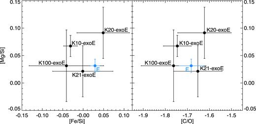
For all studied cases of planet hosts, the comparison of these key elemental ratios between their potential ‘exo-Earths’, labelled as K10-exoE, K20-exoE, K21-exoE, and K100-exoE, which are respectively corresponding to the potential habitable-zone terrestrial exoplanets orbiting the planet hosts: Kepler-10, Kepler-20, Kepler-21, and Kepler-100. Host stellar abundances are all from Schuler et al. (2015), except for Kepler-10 that is from Liu et al. (2016). The Earth (same as Fig. 4) is plotted as a reference.
3.2 Estimates of planetary interiors
Based on the recommended chemical networks of the mantle and core of a terrestrial planet, we estimate the mantle and core composition as well as the core mass fraction for these potential exo-Earths. These estimates are listed in Table 3. We also extract the information of the major components (SiO2, MgO, and FeO) in the mantle and of the core mass fraction, and then compare them in Fig. 6. It should be noted that the mantle composition in the ternary diagram of Fig. 6 has been renormalized by ignoring all minor components and assuming SiO2 + MgO + FeO = 100 wt%.
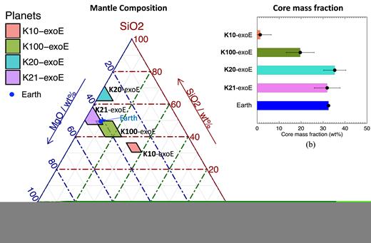
(a) A ternary diagram illustrating the estimates of the mantle composition (normalized by SiO2 + MgO + FeO = 100 wt%, adapted from Table 3) for potential exoEarths orbiting the studied host stars. The Earth’s mantle composition of SiO2, MgO, and FeO in McDonough & Sun (1995) is normalized similarly and plotted as a reference. (b) A bar graph comparing the estimates of the core molar mass fraction of these exoEarths (see Table 3). The Earth’s core mass fraction (32.5 ± 0.3 wt%) in Wang et al. (2018b) is plotted as a reference. For Kepler-10, only one of the two sets of results for its potential exoEarth is plotted here, which refers to the higher precision estimates of the host stellar abundances (i.e. Liu et al. 2016).
Estimates of the mantle and core composition as well as core mass fraction of potential habitable-zone terrestrial exoplanets (i.e. exo-Earths) orbiting the studied host stars: Kepler-10 (K10), Kepler-20 (K20), Kepler-21 (K21), Kepler-100 (K100).
| Quantity | Potential habitable-zone terrestrial exoplanets (i.e. exo-Earths)a | Pyrolite silicate Earth | ||||
|---|---|---|---|---|---|---|
| (molar wt%) | K10-exoE | K20-exoE | K21-exoE | K100-exoE | McDonough & Sun (1995) | |
| Mantle | SiO2 | 30.3 ± 2.6 | 50.7 ± 3.3 | 49.9 ± 4.9 | 40.5 ± 4.4 | 45.0 |
| CaO | 2.50 ± 0.22 | 4.39 ± 0.34 | 3.85 ± 0.38 | 2.98 ± 0.36 | 3.55 | |
| Na2O | 0.23 ± 0.02 | 0.43 ± 0.03 | 0.41 ± 0.04 | 0.41 ± 0.05 | 0.36 | |
| MgO | 29.2 ± 2.4 | 25.7 ± 3.6 | 43.3 ± 3.9 | 36.0 ± 4.0 | 37.8 | |
| Al2O3 | 3.28 ± 0.31 | – | – | 4.01 ± 0.47 | 4.45 | |
| FeO | 31.3 ± 5.1 | – | |$1.53^{+8.35}_{1.53}$| | 13.9 ± 7.9 | 8.05 | |
| NiO | 1.71 ± 0.34 | – | |$0.15^{+0.40}_{-0.15}$| | 0.95 ± 0.51 | 0.25 | |
| SO3 | 1.25 ± 0.46 | – | 0.50 ± 0.48 | 0.90 ± 0.51 | – | |
| CO2 | – | – | – | – | – | |
| Graphite | 0.28 ± 0.05 | 0.38 ± 0.05 | 0.42 ± 0.06 | 0.30 ± 0.07 | – | |
| Metals | – | 18.4 ± 10.7 | – | – | – | |
| McDonough (2014)b | ||||||
| Core | Fe | 85.7 ± 5.0 | 94.5 ± 0.6 | 94.1 ± 1.3 | 92.9 ± 1.9 | 92.33 |
| Ni | 5.25 ± 0.73 | 5.49 ± 0.63 | 4.76 ± 0.65 | 5.69 ± 0.68 | 5.62 | |
| S | 9.07 ± 5.24 | – | 1.16 ± 1.14 | |$1.40^{+1.83}_{-1.40}$| | 2.05 | |
| Core mass fraction | |$1.4^{+5.0}_{-1.4}$| | 35.3 ± 5.1 | 31.9 ± 5.9 | 19.6 ± 6.3 | 32.5 ± 0.3c | |
| (wt% planet) | ||||||
Notes.aBulk elemental compositions of these exo-Earths are from Table 1.
bMass fractions of the three elements in the core of McDonough (2014) have been renormalized under the assumption of only the three elements in the core.
cRefers to Wang et al. (2018b), in which the core mass fraction is integrated from Earth’s radial density profiles.
From Table 3 and Fig. 6, we can further identify that K21-exoE is the most Earth-like, in terms of all interior parameters we have modelled, including the mantle composition, core composition and core mass fraction. This similarity has been implied by the analyses of key elemental ratios above, but it is more conclusive and obvious here. In particular, according to the normalized mantle composition in the ternary diagram of Fig. 6, K20-exoE has the highest SiO2 (66.4 ± 4.3 wt%) and the lowest MgO (33.6 ± 4.7 wt%). The mantle rocks of K20-exoE therefore will be more enriched in pyroxene (MgSiO3) compared to other planet cases studied here (including the Earth). In contrast, K10-exoE has the lowest SiO2 (33.4 ± 2.9 wt%) and the equivalent MgO (32.2 ± 2.8 wt%), and thus its mantle rocks will potentially be more forsterite (Mg2SiO4) enriched than the others. For K21-exoE and K100-exoE, there is an overlap of their mantle compositions with that of the Earth as shown in the ternary diagram, so they would have similar mantle rocks as the Earth’s. However, as shown in the bar diagram of core mass fractions (Fig. 6b), K100-exoE has a relatively smaller core (in terms of core mass fraction) than K21-exoE and the Earth, and the latter two are comparable. This can be explained by the differences of planetary bulk compositions (Table 1), in which the mean of Fe abundance of K100-exoE (−0.17 ± 0.08 dex) is ∼1σ lower than that of K21-exoE (−0.09 ± 0.07 dex) and that of the Earth (−0.07 ± 0.02 dex) while their abundances of other major elements including O, Mg, and Si are similar.
In addition, FeO is the most enriched in the mantle of K10-exoE [while it is the least (nil) in the mantle of K20-exoE]. Namely, in comparison with other planet cases studied here, the differentiation of iron into the core of K10-exoE is the least efficient, thus leading to the smallest core (0–6.4 wt%) among the studied cases. The reason is present in its distinct host stellar abundances. Comparing with other selected planet hosts, Fe abundance in Kepler 10 (referring to Liu et al. 2016) is about 1–3σ lower while its O abundance relative to Mg and Si (i.e. O–Mg–2Si, in dex) is 1–5σ higher. As a consequence, almost all Fe in Kepler 10 is oxidized, and only a tiny amount of metallic Fe sinks into the core, thus leading to the substantially smaller core mass fraction in K10-exoE as modelled. This reveals the importance of the trade-off between oxygen and other major rock-forming elements to the exoplanetary interior modelling.
3.3 Conservative estimates
We also apply the upper and lower limits of the 3σ error bar of the best-fitting devolatilization pattern of Wang et al. (2018a) to the respective upper and lower limits of the host stellar elemental abundances. It should be noted that the 3σ is conveniently amplified over the uncertainty associated with the coefficients of the pattern; thus, the resultant 3σ range is more conservative than a range constrained by a 3σ chi-square fit. The resultant conservative estimates – ‘less depleted’ and ‘more depleted’ – are listed in Table 4.
Conservative estimates of the mantle and core composition as well as core mass fraction of any rocky exoplanet orbiting the studied host stars.
| Quantity | Less depleteda | More depletedb | |||||||
|---|---|---|---|---|---|---|---|---|---|
| (molar wt%) | K10 | K20 | K21 | K100 | K10 | K20 | K21 | K100 | |
| Mantle | SiO2 | 23.3 | 26.4 | 25.3 | 24.0 | 51.0 | 47.5 | 61.0 | 59.1 |
| CaO | 1.68 | 2.06 | 1.76 | 1.56 | 4.96 | – | – | 5.09 | |
| Na2O | 0.25 | 0.32 | 0.31 | 0.34 | 0.27 | – | – | 0.41 | |
| MgO | 22.4 | 27.6 | 22.5 | 21.4 | 26.5 | – | – | 0.55 | |
| Al2O3 | 2.17 | 2.31 | – | 2.00 | – | – | – | – | |
| FeO | 25.1 | 37.2 | 32.5 | 27.5 | – | – | – | – | |
| NiO | 1.33 | 1.90 | 1.48 | 1.51 | – | – | – | – | |
| SO3 | 2.69 | – | 2.25 | 2.40 | – | – | – | – | |
| CO2 | 4.90 | 1.07 | 5.02 | 4.35 | – | – | – | – | |
| Graphite | – | 1.01 | – | – | 0.08 | 0.07 | 0.08 | 0.07 | |
| Metals | – | – | – | – | 17.2 | 52.4 | 38.9 | 34.8 | |
| Extra O | 16.2 | – | 8.90 | 14.9 | – | – | – | – | |
| Core | Fe | – | – | – | – | 93.8 | 94.0 | 93.9 | 92.5 |
| Ni | – | – | – | – | 5.28 | 6.05 | 5.39 | 6.68 | |
| S | – | – | – | – | 0.92 | – | 0.69 | 0.86 | |
| Core mass fraction | 0 | 0 | 0 | 0 | 31.7 | 38.3 | 36.1 | 32.8 | |
| (wt% planet) | |||||||||
Notes.aApplying the upper bound of 3σ uncertainty of the Sun-to-Earth devolatilization pattern to the upper limits of host stellar abundances.
bApplying the lower bound of 3σ uncertainty of the Sun-to-Earth devolatilization pattern to the lower limits of host stellar abundances.
Though the volatile gradient of a planetary system versus the distance to its central star is still controversial (Morgan & Anders 1980; Palme 2000; Wang & Lineweaver 2016; Jin & Mordasini 2018), the dichotomy of planets from ‘rocky’ to ‘gas/icy’ or from ‘warm’ to ‘cold’ would be expected from the inward to outward in a planetary system (if those planets exist around the central star). Therefore, the ‘less depleted’ case might assemble the interior properties of ‘cold’ rocky bodies (e.g. asteroids) beyond the outer edge of the habitable zone but within the snowline of a planetary system. In contrast, the ‘more depleted’ case might be a better proxy for the interior properties of ‘warm’ rocky planets, such as the known planets Kepler-10b, Kepler-20b, Kepler-21b, and Kepler-100b, which are closer to their host stars.
4 DISCUSSION
4.1 Comparison with previous studies
The diversity of planetary interiors should be expected. Neither our conservative estimates in Table 4 nor the estimates for habitable zone terrestrial exoplanets in Table 3 should be taken as an explicit interpretation of the interiors of any existing planet orbiting these studied host stars, but only the plausible ranges constrained by different scenarios as demonstrated in the paper. The previous studies (e.g. Santos et al. 2015; Weiss et al. 2016; Brugger et al. 2017) usually state that their analyses are for an explicit planet around a parent star but this statement should be taken with caution. For example, the core mass fraction (wt%) of Kepler-10b has been previously estimated to be 27.5 ± 1.7 (Santos et al. 2015), 17 ± 11 (Weiss et al. 2016), and 10–33 (Brugger et al. 2017), which seem to approximate our ‘more depleted’ case (∼ 30) for a ‘warm’ rocky planet orbiting Kepler 10. Whereas, those previous estimates are achieved by fixing all Fe into the core (Santos et al. 2015) or relying on Mg# (=Mg/(Mg + Fe)) (Weiss et al. 2016; Brugger et al. 2017), without considering oxygen fugacity/budget that controls the oxidation state of a planet. If one generalizes those fixed assumptions to potential rocky planets at different distances to the same star, the same chemistry and interior structure for these planets would result. Although taking into account planetary mass and radius, the modelling results could be more specific to such planets, but the results would still be degenerate to the degree to which oxygen fugacity/budget would vary in the disc. When targeting a potentially habitable planet for further characterization with future missions, we should particularly be cautious with this kind of ‘explicit’ claims, which may only assemble one scenario of possible interior properties of rocky exoplanets orbiting at different distances to their host stars. The depletion of oxygen in Kepler-10 planets relative to the host star is not considered in Dorn et al. (2017a), but they assume Fe/Simantle = [0, Fe/Sistar] (uniform distribution), implicitly resulting in varied differentiation of Fe into the core, which somehow assembles the consideration of oxygen fugacity/budget in determining the fractionation of Fe between the mantle and core.
Complex mineral compounds [e.g. (Mg,Fe)SiO3, (Mg,Fe)2SiO4] have been presumed to be present in the mantle rocks of super-Earths in the studies of Santos et al. (2015), Weiss et al. (2016), Brugger et al. (2017), and Hinkel & Unterborn (2018). However, for exoplanets that are larger than Earth, their mineralogies may not be sensibly interpretable in using the equation-of-state (EoS) parameters measured with respect to the pressure and temperature regime of the Earth (Mazevet et al. 2015). Therefore, we have chosen to use first-order mineral forms (i.e. oxides) for our modelling of mantle and core compositions. To first order, the planetary chemistry does not change, just the mineralogy. This practice is also in line with Dorn et al. (2015, 2017a,b). When we have the observational information of atmospheric thickness/composition of a terrestrial exoplanets at the era of JWST, we will know better the plausible pressure range associated with the solid regime of such a planet. With the further progress of ultrahigh pressure and temperature experiments of the physical state and properties of minerals, we can be more confident in our modelling of more complex exoplanetary mineralogies.
4.2 Requirement on the precisions of host stellar abundances
Hinkel & Unterborn (2018) modelled the mineralogy for fictive planets around the 10 stars closest to the Sun and concluded that abundance uncertainties need to be on the order of [Fe/H] < 0.02 dex, [Si/H] < 0.01 dex, [Al/H] < 0.002 dex, [Mg/H], and [Ca/H] < 0.001 dex, in order to distinguish different planetary populations orbiting their sample of 10 stars. Based on our modelling results above, we have demonstrated that the interior composition and structure of those potential terrestrial exoplanets as studied can be distinguished from each other, by using the current, high-precision host stellar abundances (with a typical uncertainty of ≲0.04 dex). This is a much less strict requirement on the precisions of host stellar abundances. It is legitimate to strive for much more precise stellar abundances (as well as planetary mass and radius measurements) and thus to improve the interior modelling accuracy. However, we should also be realistic, since precisions of host stellar abundances depend not only on modelling techniques but also on characteristics of target stars and observation exposure time. A careful weighing of costs and benefits is crucial for the success of a space mission – as noted in Dorn et al. (2015) – like TESS/JWST and follow-up observations. Improving the exoplanetary interior modelling approaches may be an alternative and more sensible way to achieve better characterization of planetary chemistry and structures in the coming decade.
4.3 Limitations
The success of a theoretical model is subject to the limitations of premises/assumptions. First, as mentioned earlier, our model is limited by how representative the Sun-to-Earth devolatilization pattern is for terrestrial planets in general. If we had a more exhaustive devolatilization model built on the comprehensive comparisons of the compositions of all inner Solar system rocky bodies, gas giants, and icy bodies (including a variety of comets), we would have more accurate modelling results for exoplanetary chemistry. However, it is unclear to what extent the appearance of super-Earths in the proximity of their host stars (radically different to the scenario of the Solar system) would change the devolatilization process and thus the bulk compositions of their planet companions in the circumstellar habitable zone. We have just scratched the surface of considering devolatilization in modelling exoplanetary chemistry and interiors, and this issue remains degenerate. Secondly, our approach to oxidize elements by following a sequence of oxidation might be worth revisiting if the oxidation of elements is done in parallel (simultaneously), not in sequence. In the parallel case, all rock-forming elements would compete to be oxidized to some extent. It is unclear how significant the end-member oxides resulting from this competition would be in comparison with those resulting from an assumed sequence. Thirdly, our modelling results are also limited to the current dimensionality of the model, namely, two-component overall structure (an iron alloy core and a silicate mantle), with no water layer (or oceans) or gas layer (or H/He envelopes) considered yet. With the upcoming addition of planetary atmosphere observations, we are expecting to expand the dimensionality of our model to be inclusive of water/gas reservoirs in a terrestrial exoplanet by taking into account important atmospheric information, pressure and temperature associated with the actual size of the solid regime of a planetary body.
Nevertheless, we envisage that if a terrestrial planet is confirmed in the habitable zone around the host stars studied here, our modelling results of the mantle and core compositions as well as core mass fractions listed in Table 3 are good first-order estimates of the interior composition and structure of that planet. We also emphasize that the purpose of this work is to set more appropriate initial conditions for modelling exoplanetary interiors, especially with the addition of a ‘devolatilization’ process into the host stellar abundances. These enhanced constraints can be potentially transferable to some recent models (e.g. Brugger et al. 2017; Dorn et al. 2017a; Dorn et al. 2017b; Unterborn et al. 2018) and thus enhance the model performance. Additional data (e.g. atmospheric information and applicable EoS parameters for all considered compositions) are required for further studies to decipher the detailed interior structure and chemistry, surface conditions and thus habitability of such terrestrial exoplanets.
5 SUMMARY AND CONCLUSIONS
Devolatilization (i.e. depletion of volatiles) plays an essential role in the formation of rocky planetary bodies from a stellar nebular disc (Bland et al. 2005; Norris & Wood 2017). The terrestrial devolatilization pattern of Wang et al. (2018a) has been applied in this study to infer the bulk elemental composition of potential terrestrial exoplanets that are presumed to exist within the circumstellar habitable zones. The inferred planetary bulk composition (rather than the host stellar abundances) provides improved principal constraints to model the interior composition and structure of such planets. Other recommended constraints include (i) the mantle chemical network (SiO2–CaO–Na2O–MgO–Al2O3–FeO–NiO–SO3, in order of the ease of oxidation); (ii) the core chemical network (Fe–Ni–S alloy, Fe/Ni constrained at 18 ± 4 by number).
By applying these constraints to the Sun, we show that the mantle and core compositions of our model Earth are supported by the independent measurements/estimates for the planet Earth in the literature. By applying our modelling approach to selected planet hosts (Kepler-10, Kepler-20, Kepler-21, and Kepler-100), we find that the interior compositions and structures of potential terrestrial exoplanets in the habitable zones around these stars are diverse. For example, the estimates of core mass fraction range from about 1.5 wt% (K10-exoE) to about 35 wt% (K20-exoE). This diversity can be explained from the differences in their host stellar abundances. With respect to the interior estimates (i.e. mantle and core compositions as well as core mass fraction), we conclude that a potential terrestrial planet orbiting Kepler-21 would be the most Earth-like while one orbiting Kepler-10 would be the least (among the cases we studied). High-precision host stellar abundances are critical for exoplanetary interior modelling. A precision better than ∼0.04 dex is necessary to assess the similarity of exoplanetary interiors to the Earth’s, based on our modelling approach.
In summary, for more accurate estimates of interior composition and structure of terrestrial exoplanets, it is essential to enhance the initial conditions pertinent to planetary bulk composition and interior chemical models, in addition to the increasingly higher precision measurements of host stellar photosphere and planetary mass and radius, alongside with the progressive observations of planetary atmospheres, in the era of TESS, PLATO, and JWST.
ACKNOWLEDGEMENTS
We thank the anonymous referee whose comments greatly improved the quality of the paper. We acknowledge valuable discussions with William F. McDonough, Thomas Nordlander, and Stephen Mojzsis. HSW was supported by the Prime Minister’s Australia Asia Endeavour Award (No. PMPGI-DCD-4014-2014) from Australian Government Department of Education and Training. FL was supported by the Märta and Eric Holmberg Endowment from the Royal Physiographic Society of Lund. This work has made use of the Hypatia Catalog Database at hypatiacatalog.com, which was supported by NASA's Nexus for Exoplanet System Science (NExSS) research coordination network and the Vanderbilt Initiative in Data-Intensive Astrophysics (VIDA).
REFERENCES
APPENDIX A: COMPUTATIONAL DETAILS OF ELEMENTAL FRACTIONATION BETWEEN THE MANTLE AND THE CORE3
The elemental fractionation is based on the recommended chemical networks for the mantle and core of a terrestrial planet in Sections 2.2 and 2.3. The computational procedure illustrated in Fig. 3 is described in detail in the following.
First, oxidize Si, Ca, Na, Mg, and Al (in order of the decreasing ease of oxidation addressed in Section 2.3) to form oxides: SiO2, CaO, Na2O, MgO, and Al2O3, respectively. For each element, assess the sufficiency of O atoms: (i) if the budget of (remaining) O atoms is not stoichiometrically sufficient to fully oxidize the element, then the non-oxidized part of the element’s atoms and the atoms of the subsequent elements (up to Al) will be deemed as ‘metals’ in the mantle; (ii) otherwise (namely, all atoms of an element can be fully oxidized), the oxidation process will be performed on the subsequent elements one by one (up to Al), unless the remaining O atoms have been exhausted.
Secondly, fractionate Fe, Ni, and S between the mantle and the core, for two scenarios:
If the remaining O atoms (after having oxidized Si, Ca, Na, Mg, and Al) are still stoichiometrically sufficient to fully oxidize Fe, Ni, and S into the form of FeO, NiO, and SO3, then there will be no Fe, Ni, or S fractionated into the core, and a coreless planet will form. The leftover oxygen atoms may oxidize the stoichiometric amount of C atoms to form CO2 in the phase of carbonates, then the remaining C atoms are present in the phase of graphite in the mantle. However, if the number of the leftover oxygen atoms is more than that of C atoms, all C atoms will be oxidized to form CO2 and the extra O is assumed to be present in the mantle to oxidize other minor elements that are not investigated in this work.
- Complementarily, if the remaining O atoms are not stoichiometrically sufficient to fully oxidize Fe, Ni, and S, then the atoms of the three elements will be fractionated between the mantle and the core, and all C atoms will be present in the phase of graphite in the mantle. The upper limits of atomic abundances of Ni and S in the phase of NiO and SO3 in the mantle are assumed to be equal to their respective planetary bulk abundances (after being devolatilized from the host stellar abundance). Their lower limits are assumed to be 0. Assume the abundances of Ni and S in the mantle can be any value within their respective upper and lower limits, following a uniform distribution (denoted as ‘u’):(A1)\begin{eqnarray*} N_{\textrm{Ni, mantle}} =[0, N_{\textrm{Ni, bulk}}]_u \end{eqnarray*}(A2)\begin{eqnarray*} N_{\textrm{S, mantle}} =[0, N_{\textrm{S, bulk}}]_u. \end{eqnarray*}
On the basis, we use the constraint Fe/Ni = 18 ± 4 in the core (as addressed in Section 2.3) to verify the series of Fe/Ni ratios as computed from each pair of Ni and S drawn from their respective uniform distributions (here, we draw 105 times). Only computations matching this constraint are deemed as valid estimates.
Then in combination with the atomic masses, these mantle and core abundances (by number) can be converted to the molar masses. The core (molar) mass fraction is the total molar mass in the core divided by the sum of the total molar masses in both the mantle and the core.
The process above is iterated for each combination of planetary elemental abundances, by 2 × 10⁴ Monte Carlo simulations assuming that each element’s abundance (within its uncertainty) follows a Gaussian distribution. The results corresponding to the best fit of the pattern and the mean of each input elemental abundance are reported as the mean values of the modelling results (i.e. mantle composition, core composition, and core mass fraction) in Tables 2 and 3. The error bar associated with a mean value corresponds to the standard deviation of the population of the modelling results for that quantity. The distribution of the modelling results for FeO, NiO, and SO3 in the mantle and Fe, Ni, and S in the core as well as the core mass fraction may be asymmetric around their corresponding mean values. In this case, the standard deviation of the population of the modelling results for such a quantity is not an accurate but conservative estimate for the uncertainty on the mean value of the quantity. If the standard deviation may cause the lower limit of the quantity to be negative, then the lower limit is set to be zero. As such, the error bars of some quantities in Tables 2 and 3 are asymmetric.
Footnotes
NASA Exoplanet Archive, https://exoplanetarchive.ipac.caltech.edu, which is operated by the California Institute of Technology, under contract with the National Aeronautics and Space Administration (NASA) under the Exoplanet Exploration Program.
Elements with relatively high equilibrium condensation temperatures (≳1360 K) and they are resistant to heat/irradiation/impact.
