


Abstract
The low-order kinematic moments of galaxies, namely bulk flow and shear, enables us to test whether theoretical models can accurately describe the evolution of the mass density field in the nearby Universe. We use the so-called ηMLE maximum likelihood estimator in log-distance space to measure these moments from a combined sample of the 2MASS Tully–Fisher (2MTF) survey and the cosmicflows-3 (CF3) compilation. Galaxies common between 2MTF and CF3 demonstrate a small zero-point difference of −0.016 ± 0.002 dex. We test the ηMLE on 16 mock 2MTF survey catalogues in order to explore how well the ηMLE recovers the true moments, and the effect of sample anisotropy. On the scale size of 37 h−1 Mpc, we find that the bulk flow of the local Universe is 259 ± 15 km s−1 in the direction is (l, b) = (300 ± 4°, 23 ± 3°) (Galactic coordinates). The average shear amplitude is 1.7 ± 0.4 h km s−1 Mpc−1. We use a variable window function to explore the bulk and shear moments as a function of depth. In all cases, the measurements are consistent with the predictions of the Λ cold dark matter (ΛCDM) model.
1 INTRODUCTION
In the local Universe, the gravitational effects of mass density fluctuations exert perturbations on galaxies’ redshifts on top of Hubble’s Law, called ‘peculiar velocities’. The dipole and the quadruple of the peculiar velocity field, namely ‘bulk flow’ and ‘shear’, respectively, enable us to trace the matter density fluctuations and test whether the cosmological model accurately describes the motion of galaxies in the nearby Universe.
In previous work related to the measurement of the bulk and shear moments (Staveley-Smith & Davies 1989; Jaffe & Kaiser 1995; Willick & Strauss 1998; Parnovsky et al. 2001; Feldman, Watkins & Hudson 2010; Hong et al. 2014; Scrimgeour et al. 2016; Qin et al. 2018), the results largely agree with the ΛCDM prediction. However, some studies have measured large values for the bulk flow, in apparent disagreement with the ΛCDM prediction. For example, Watkins, Feldman & Hudson (2009) measure 407 ± 81 km s−1 on the scale size of 50 h−1 Mpc.
The bulk and shear moments are usually measured in velocity space (|$v$|-space) or log-distance space (η-space). In |$v$|-space, the main measurement techniques are (Kaiser 1988; Sarkar, Feldman & Watkins 2007; Watkins et al. 2009; Feldman et al. 2010; Hong et al. 2014): log-linear χ2 minimization, minimum variance (MV) estimation and maximum likelihood estimation (MLE). Some of these |$v$|-space estimation techniques assume that the measured peculiar velocities have Gaussian errors, which is not the case for the usual estimator of peculiar velocity. Watkins & Feldman (2015) therefore introduced a peculiar velocity estimator which has Gaussian errors and, under some circumstances is unbiased. Alternatively, as shown by previous authors including Nusser & Davis (1995, 2011) and Qin et al. (2018), the bulk and shear moments in the local Universe can be measured in η-space using the ‘ηMLE’ technique. Nusser & Davis (2011) convert the model bulk flow into magnitudes analytically, using linear approximations, then convert to log-distance ratio and compare to the measurements, while Qin et al. (2018), convert the model bulk flow into log-distance ratio numerically without any approximations, then compare to the measurements.
In this work, we extend the ηMLE in Qin et al. (2018) to quadrupole (shear) measurements and, through weighting functions, compare the measured shear moments with ΛCDM prediction at different depths. We measure the bulk and shear moments from the combined dataset of cosmicflows-3 (CF3; Tully, Courtois & Sorce 2016) and 2MASS Tully–Fisher (2MTF; Hong et al. 2014).
The paper is structured as follows: in Section 2, we introduce the data: 2MTF, CF3, and their combination. The theory associated with the low-order moments (bulk and shear) is introduced in Section 3. In Section 4, we summarize how these are estimated from the data. In Section 5, we discuss the bulk and shear moments obtained from the 2MTF mocks. The final results are presented in Section 6. We provide a conclusion in Section 7.
This paper assumes spatially flat cosmology with parameters from the Planck Collaboration XVI (2014): Ωm = 0.3175, σ8 = 0.8344, ΩΛ = 0.6825, and H0 = 100 h km s−1 Mpc−1. We use these parameters to calculate the expected ΛCDM bulk flow and shear as well as the comoving distances.
2 DATA
2.1 CF3 and 2MTF
cosmicflows-3 (CF3) is a full-sky compilation of distances and velocities (Tully et al. 2016), containing 17 669 galaxies reach |$cz = 34\, 755$| km s−1. The data sources are heterogeneous, and include distances obtained from the luminosity-linewidth (Tully–Fisher) relation, the Fundamental Plane (FP), surface-brightness fluctuations, from Type Ia supernova (SNIa) observations, the tip of the Red Giant Branch (TRGB), with the largest recent increment being the FP sample of the Six-degree-Field Galaxy Survey (6dFGS) of Springob et al. (2014). We removed those galaxies with CMB frame redshift lower than 600 km s−1, leaving 17 407.
2MTF is a Tully–Fisher sample derived from the Two Micron All-Sky Survey (2MASS). The Tully–Fisher relation is measured using H i rotation widths (Springob et al. 2005; Haynes et al. 2011; Hong et al. 2013; Masters et al. 2014) for galaxies at redshifts measured in the 2MASS Redshift Survey (Huchra et al. 2012). The final 2MTF catalogue contains 2 062 galaxies with a redshift cut 600 km s−1 < cz < 1.2 × 10⁴ km s−1. The 2MTF K-band magnitude limit is 11.25 mag.
2.2 The combination of CF3 and 2MTF
The combination of CF3 and 2MTF data offers the following advantages. First, the combined data set is much deeper than 2MTF alone (CF3 extends out to three times the redshift of 2MTF). Secondly, the combined data set is more isotropic than CF3 alone (the projected sky density of CF3 is greater in the southern sky by a factor of 2.4, and the projected density of 2MTF is greater in the northern sky by 1.6).
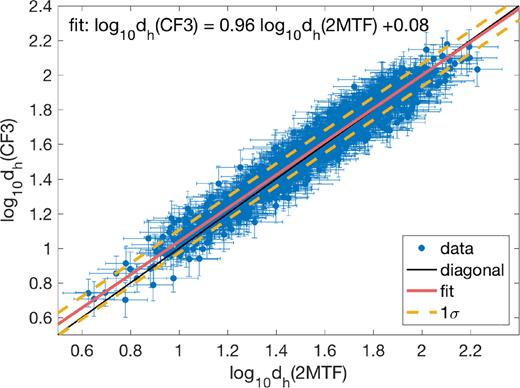
Comparing the CF3 distances to the 2MTF distances for 1 096 common galaxies. The expected 1:1 relation for perfect agreement is shown in the solid black line. The hyperfit line is shown in the solid red line. The ±1σ is indicated by the yellow dashed lines, and σ = 0.07.
Removing the 1 117 common galaxies from CF3, and adding a zero-point correction of −0.016 to the log-distance ratio data in CF3, we obtain a combined data set, which has 18 352 galaxies. The sky coverage and the redshift distribution of the combined CF3 and 2MTF is shown in Figs 2 and 3, respectively.
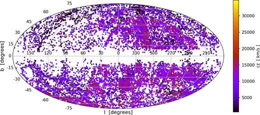
Distribution of 18 352 galaxies in the combined 2MTF and CF3 data set in Galactic coordinates. The galaxy redshift is indicated by the colour of the points, based on the right-hand colour bar. The majority of galaxies lie at recession velocities cz < 16 000 km s−1.
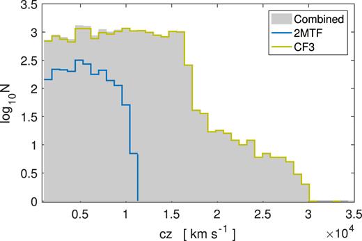
The redshift (in CMB frame) distribution of the datasets. The light-green/yellow and the blue line are for the CF3 and 2MTF data, respectively. The Combined dataset is represented by the grey bars.
3 BULK FLOW AND SHEAR MOMENTS
4 MAXIMUM LIKELIHOOD ESTIMATION
To preserve the Gaussian nature of the measurement errors, there are two methods that can be applied to obtain maximum likelihood estimates of the bulk flow velocity and shear moments.
The first (ηMLE) calculates the model log-distance ratio from the model Up and compares to the measured value (Nusser & Davis 1995, 2011; Qin et al. 2018).
The second method (|$w$|MLE) converts the measured η into |$v$|-space to obtain the peculiar velocities, |$v$| using the PV estimator of Watkins & Feldman (2015), then compares to the model Up under the assumption that the measured |$v$| has Gaussian error (Kaiser 1988).
One caveat is that the PV estimator in Watkins & Feldman (2015) only strictly estimates an unbiased peculiar velocity under the assumption that the cz of the galaxy is much greater than the true peculiar velocity (not the measured peculiar velocity) for that galaxy (Watkins & Feldman 2015). By contrast, the ηMLE can avoid assumptions about the galaxy’s unknown true PV compared to its redshift.
4.1 ηMLE
The maximum likelihood Up cannot be obtained analytically due to the non-linear relationship between the model Up and the model predicted log-distance ratio. Instead, we follow the method of Qin et al. (2018), combining flat priors on the σ⋆ and Up (excluding Qzz) with the likelihood in equation (15), enabling us to write the posterior probability of these nine independent parameters given the cosmological model and the data. Here, we use the Metropolis–Hastings Markov chain Monte Carlo (MCMC) algorithm with flat priors in the interval Bi ∈ [−1200, +1200] km s−1 and Qij ∈ [−100, +100] h km s−1 Mpc −1 to explore the posterior.
Feldman et al. (2010) use the MV method to estimate Up. In their estimator, they set Qzz as an independent component rather than using equation (7) to compute Qzz from Qxx and Qyy. In our paper, we also tested the ηMLE on mocks by setting Qzz as an independent component (see Appendix A), but found this led to larger reduced χ2.
4.2 wMLE: estimation in v-space
5 BULK AND SHEAR MOMENTS IN THE 2MTF MOCKS
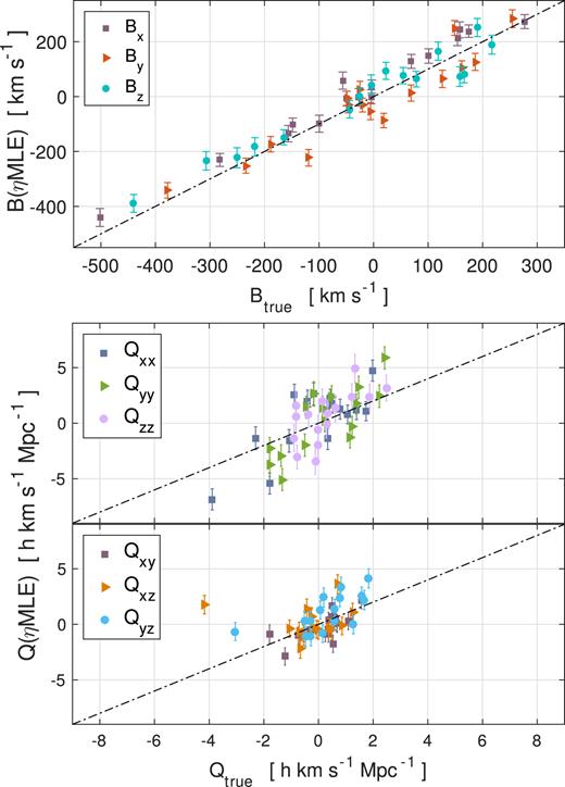
In order to test how well the ηMLE and the |$w$|MLE are expected to recover the true moments from the observational data, we applied the two estimators to 16 mock 2MTF catalogues (Howlett et al. 2017). We use the SURFS simulations (Elahi et al. 2018) and the GiggleZ (Poole et al. 2015) to generate these mocks. The SURFS simulation uses cosmological parameters of Ωm = 0.3121, Ωb = 0.0488, and h = 0.6751. while the GiggleZ simulation uses cosmological parameters of Ωm = 0.273, Ωb = 0.0456, and h = 0.705. This also allows us to explore whether the two estimators give consistent answers under different cosmologies. Each mock catalogue contains |$\sim 2\, 000$| galaxies, and matches the survey geometry (i.e. sky coverage and the distance distribution) and the selection function of the 2MTF survey (Qin et al. 2018).

The measured bulk flow for the 16 2MTF mocks in equatorial coordinates. The upper and bottom panels are for the |$w$|MLE estimator and the ηMLE estimator, respectively.
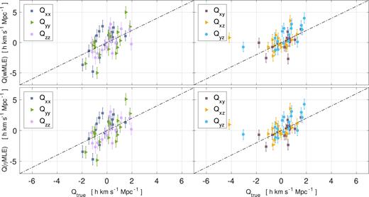
The measured shear moments for the 16 2MTF mocks. The (x, y, |$z$|) measurements are in equatorial coordinates. The upper and lower panels are for the |$w$|MLE estimator and the ηMLE estimator, respectively.
Generally, for both the bulk flow measurements and the shear measurements, the |$w$|MLE and ηMLE perform similarly and return unbiased measurements of bulk flow and shear moments. However, due to the Watkins & Feldman (2015) estimator having a necessary assumption of |$v$|true ≪ cz, some systematic errors are introduced for the closest galaxies in the mocks. As a result, the |$\chi ^2_{\mathrm{ red}}({\bf B})$| of |$w$|MLE is slightly higher compared to the ηMLE. Overall, we find ηMLE performs better than |$w$|MLE for the 2MTF mocks, and for the subsequent parts of this paper, ηMLE is the one we shall adopt to measure the bulk flow and shear moments from the data sets.
The reasons for the reduced chi-squared values far from 1 are most likely due to: (i) the assumption that the standard deviation of true velocities in the mocks is σ⋆ (or ε⋆, n in the ηMLE method); (ii) the fitted values of bulk and shear flow are weighted in a different manner to the ‘true’ values, leading to different effective depths; and (iii) the moment model is only a low-order approximation of a more complex velocity field.
6 RESULTS AND DISCUSSION
6.1 Results and comparison with ΛCDM theory
The resultant bulk and shear moments measurements (in Galactic coordinates) for 2MTF, CF3, and the combined data are presented in Table 1. The measurement errors of the bulk flow velocity and shear moments for the combined data set (and CF3) are much smaller compared to 2MTF. This is mainly due to the combined data set covering a much larger cosmological volume. CF3 also combines distances using the weighted average of multiple measurements, if available.
Bulk flow and shear moments measurements for 2MTF, CF3, and the combined data set in Galactic coordinates. The CRMS column gives expected cosmic variance due to ΛCDM. The last row lists the depth of the measurement.
| 2MTF | CF3 | Combined | ||||
|---|---|---|---|---|---|---|
| ηMLE | CRMS | ηMLE | CRMS | ηMLE | CRMS | |
| Bx (km s−1) | 130.6 ± 39.5 | ±164.8 | 134.5 ± 17.4 | ±160.4 | 120.6 ± 17.7 | ±155.6 |
| By (km s−1) | −340.3 ± 37.0 | ±172.1 | −282.7 ± 15.7 | ±169.4 | −206.5 ± 16.1 | ±164.2 |
| B|$z$| (km s−1) | 85.4 ± 30.5 | ±185.6 | 76.6 ± 11.9 | ±178.3 | 99.5 ± 12.1 | ±173.4 |
| Qxx (h km s−1 Mpc−1) | 3.69 ± 1.35 | ±2.53 | 0.73 ± 0.43 | ±1.78 | 2.12 ± 0.44 | ±1.68 |
| Qxy (h km s−1 Mpc−1) | −4.16 ± 1.16 | ±1.45 | −1.41 ± 0.36 | ±0.95 | −1.16 ± 0.36 | ±0.89 |
| Qxz (h km s−1 Mpc−1) | −0.96 ± 0.97 | ±1.32 | 1.13 ± 0.28 | ±0.86 | 0.17 ± 0.27 | ±0.80 |
| Qyy (h km s−1 Mpc−1) | 0.36 ± 1.30 | ±3.20 | 0.83 ± 0.41 | ±1.84 | 1.94 ± 0.41 | ±1.74 |
| Qyz (h km s−1 Mpc−1) | −1.47 ± 1.01 | ±1.54 | −0.14 ± 0.29 | ±0.89 | 0.47 ± 0.29 | ±0.83 |
| Qzz (h km s−1 Mpc−1) | −4.05 ± 1.18 | ±2.68 | −1.56 ± 0.36 | ±2.02 | −4.06 ± 0.36 | ±1.85 |
| dMLE (h−1 Mpc) | 32 | 35 | 37 | |||
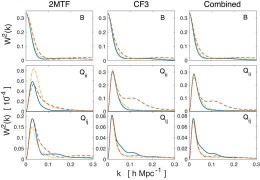
The window functions for 2MTF, CF3, and the combined data set, all in Galactic coordinates. In the top panels are the bulk flow x (blue solid curve), y (yellow dot-dashed curve), and |$z$| (red dashed curve) components. In the middle panels are the Qxx (blue solid curve), Qyy (yellow dot-dashed curve), Qzz (red dashed curve) components. In the bottom panels are the Qxy (blue solid curve), Qxz (yellow dot-dashed curve), Qyz (red dashed curve) components. The left-hand side panels are for 2MTF, the middle panels are for CF3, the right-hand side panels are for the combined data set.
The estimation procedure of CMRS follows the arguments in Feldman et al. (2010) (see also Watkins et al. 2009; Scrimgeour et al. 2016). To reiterate, to obtain the estimates of the CMRS expected within our survey under the ΛCDM cosmological model, we perform the following steps:
Use the positions and errors of galaxies within the 2MTF (CF3) survey to calculate the weight factors in equation (31).
Combine these with the fmn term in equation (30) (which also only depends on the 2MTF (CF3) galaxy positions) to calculate the window function of the data.
Integrate this window function along with the ΛCDM power spectrum to calculate the matrix Rpq in equation (29).
The CMRS values are then given by the diagonal elements of Rpq.
From Table 1, for the CF3, 2MTF and the combined sample, we find that the majority of our Qij measurements are consistent with the CRMS calculated from ΛCDM theory. After combining the CRMS predictions with measurement errors, the largest deviations are the Qxy component in 2MTF at 2.2σ and the Qzz component in the combined data set at 2.2σ too.
The ηMLE measured bulk flows are compared to the prediction of ΛCDM and its cosmic variance.
| ΛCDM |B| (km s−1) | ηMLE |B| (km s−1) | |
|---|---|---|
| CF3 | 238|$^{+122}_{-104}$| | 322 ± 15 |
| 2MTF | 243|$^{+125}_{-106}$| | 374 ± 36 |
| Combined | 231|$^{+118}_{-101}$| | 259 ± 15 |
| ΛCDM |B| (km s−1) | ηMLE |B| (km s−1) | |
|---|---|---|
| CF3 | 238|$^{+122}_{-104}$| | 322 ± 15 |
| 2MTF | 243|$^{+125}_{-106}$| | 374 ± 36 |
| Combined | 231|$^{+118}_{-101}$| | 259 ± 15 |
6.2 Cosmic flow as a function of depth
The bulk flow amplitudes, measured from 2MTF and the CF3 individually and combined, are plotted against the survey depth in Fig. 7. Usually, comparing bulk flow measurements between different surveys on a single figure is difficult, since those surveys have differing survey geometries and depths. Therefore, it is necessary to standardize the window function, and in this paper, we used the spherical top-hat window function: |$\mathcal {W}(k)=3(\sin kR-kR\cos kR)/(kR)^3$|. In Fig. 7, we also compare our bulk flow measurements with the measurements of others (Watkins et al. 2009; Colin et al. 2011; Dai, Kinney & Stojkovic 2011; Nusser & Davis 2011; Turnbull et al. 2012; Ma & Scott 2013; Hong et al. 2014; Scrimgeour et al. 2016; Qin et al. 2018). The black solid curve represents the most likely bulk flow predicted by the ΛCDM using the spherical top-hat window function. From Fig. 7, we find most of the measured bulk flows are consistent with the ΛCDM prediction at the 68 per cent confidence level.
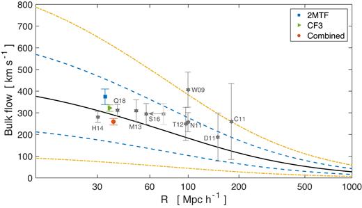
The ηMLE measured bulk flow amplitudes (filled circles •) for 2MTF, CF3, and the combined data set are compared to values from other authors. The most probable bulk flow from the ΛCDM prediction is shown as the solid line. The yellow and blue dashed lines indicate 95 per cent and 68 per cent confidence levels, respectively. Other measurements are indicated by the grey stars (⋆) (Q18: Qin et al. 2018; H14: Hong et al. 2014; T12: Turnbull et al. 2012; W09: Watkins et al. 2009; N11: Nusser & Davis 2011; M13: Ma & Scott 2013; D11: Dai et al. 2011; C11: Colin et al. 2011; S16: Scrimgeour et al. 2016). Following Scrimgeour et al. (2016), W09 and T12 are plotted at twice their quoted radius since they use Gaussian windows. To account for the half-sky coverage of 6dFGSv, the S16 (Scrimgeour et al. 2016) measurement is shifted as shown by the grey arrow.
In Fig. 8, the bulk flow directions are compared in Galactic coordinates. The bulk flow directions from different surveys are mainly in agreement except S16 (Scrimgeour et al. 2016). This discrepancy appears to come from their imperfect Malmquist bias correction to the 6dFGSv data, based on the assumption that peculiar velocities, estimated from equation (11), have Gaussian errors (see Qin et al. 2018). The bulk flow direction converges towards the CMB dipole, and appears to be due to local effects combined with more distant gravitational perturbations, including the Shapley supercluster.
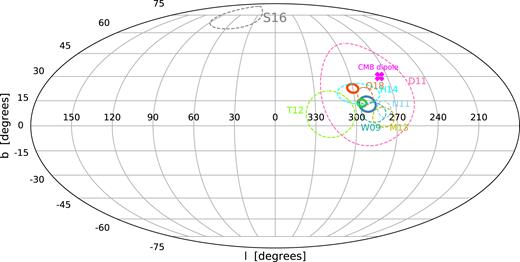
The direction of bulk flow from different measurements are compared in Galactic coordinates. The ηMLE results for 2MTF, CF3, and the combined data set are shown in the blue, green, and the red solid circles, respectively. The coloured dashed circles indicate other recent measurements (Q18: Qin et al. 2018; H14: Hong et al. 2014; T12: Turnbull et al. 2012; W09: Watkins et al. 2009; N11: Nusser & Davis 2011; M13: Ma & Scott 2013; D11: Dai et al. 2011; S16: Scrimgeour et al. 2016). The 1σ error is indicated by the radius of the circles. The CMB dipole direction is shown as the pink cross.
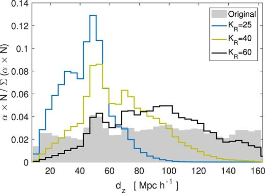
The distribution of d|$z$| setting KR = 25, 40, and 60, respectively. The grey bars are the original distribution of d|$z$| without any weighting.
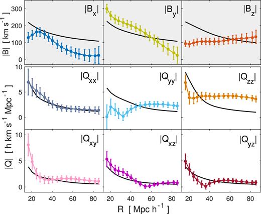
The absolute amplitude of the moments as a function of survey depth. The upper panels are for the bulk flow, the middle panels are for the diagonal elements of the shear tensor, and the bottom panels are for the non-diagonal elements of the shear tensor. The black solid curves are the ΛCDM CRMS predictions for each moment. The measurement points for the components are highly correlated, so their covariance must be taken into account when comparing to the black curves.
The χ2 and probability P(> χ2) of the measured moments at different depths. The degrees of freedom for B, Q and U are 3, 5, and 8, respectively.
| R | B | Q | U | |||
|---|---|---|---|---|---|---|
| h−1 Mpc | χ2 | P | χ2 | P | χ2 | P |
| 20 | 2.284 | 0.52 | 7.051 | 0.22 | 9.0160 | 0.34 |
| 28 | 2.793 | 0.42 | 4.774 | 0.44 | 6.7161 | 0.57 |
| 36 | 2.761 | 0.43 | 3.989 | 0.55 | 6.2778 | 0.62 |
| 45 | 2.454 | 0.48 | 3.778 | 0.58 | 6.2926 | 0.61 |
| 54 | 2.123 | 0.55 | 5.204 | 0.39 | 8.1539 | 0.42 |
| 58 | 1.979 | 0.58 | 6.083 | 0.30 | 9.3231 | 0.32 |
| 63 | 1.882 | 0.60 | 6.869 | 0.23 | 10.3767 | 0.24 |
| 66 | 1.803 | 0.61 | 7.327 | 0.20 | 10.9342 | 0.21 |
| 71 | 1.726 | 0.63 | 7.780 | 0.17 | 11.4380 | 0.18 |
| 76 | 1.671 | 0.64 | 7.804 | 0.17 | 11.1989 | 0.19 |
| 81 | 1.675 | 0.64 | 7.685 | 0.17 | 10.7017 | 0.22 |
| 85 | 1.739 | 0.63 | 7.029 | 0.22 | 9.7784 | 0.28 |
7 CONCLUSIONS
We have measured the bulk and shear moments in the individual and combined 2MTF and CF3 surveys. We applied the ηMLE to the catalogues in order to preserve the Gaussian nature of the measurement errors of the peculiar velocities. Using the galaxies common between 2MTF and CF3, we demonstrate a small zero-point difference of −0.016 ± 0.002 dex.
We have tested the ηMLE on 2MTF mocks and compare to the |$w$|MLE results. We find ηMLE performs better than |$w$|MLE in both the bulk and shear moment estimation. In addition, by performing tests on anisotropic mocks, we found that leaving Qzz (or the trace of shear tensor) as a free parameter in the MCMC routine of ηMLE is not desirable, and increases the measurement error of Qzz significantly.
We compare the measured bulk and shear components to the predictions from ΛCDM model and the measurements to be consistent with the ΛCDM prediction, with no substantial deviation from the cosmic RMS values predicted by ΛCDM. Using the combined data set, we have also explored the change of bulk and shear moments with survey depth and again find consistency with ΛCDM at all depths between 20 and 85 Mpc h−1. Using the combined sample, we measured the amplitude (depth) of the bulk flow to be 259 ± 15 km s−1 (37h−1 Mpc), the result again being consistent with the ΛCDM prediction at the 68 per cent confidence level.
ACKNOWLEDGEMENTS
FQ has received financial support from China Scholarship Council (CSC). TH is supported by the Open Project Program of the Key Laboratory of FAST, NAOC, Chinese Academy of Sciences. Parts of this research were conducted by the Australian Research Council Centre of Excellence for All-sky Astrophysics (CAASTRO), through project number CE110001020 and the Australian Research Council Centre of Excellence for All Sky Astrophysics in 3 Dimensions (ASTRO 3D), through project number CE170100013.
Footnotes
The upper and lower limits mean that the integral of equation (32) in the interval [Bp − 0.356σB, Bp + 0.419σB] is 0.68. The integral in the interval [Bp − 0.619σB, Bp + 0.891σB] is 0.95. The interesting question is if we were to calculate the bulk flow around N random ΛCDM observers, what would be the expected value of the bulk flow (the answer is Bp) and where would 68 per cent (95 per cent) of the measurements lie about this point. Then comparing this statistic to our measured local bulk flow as a test of whether or not our measurement would be expected within a ΛCDM universe.
REFERENCES
APPENDIX A: SETTING Qzz AS AN INDEPENDENT PARAMETER IN ηMLE
In the MCMC routine of ηMLE, by setting Qzz as an independent shear component, we measured the bulk flow for the 16 2MTF mocks in equatorial coordinates, and compare to the true bulk flow in the top panel of Fig. A1. We find |$\chi ^2_{\mathrm{ red}}({\bf B}) = 3.73$|. The measured shear moments from the mocks are shown in middle and bottom panels of Fig. A1. Correspondingly, the true shear moments is calculated directly from equation (25) without removing the trace. The |$\chi ^2_{\mathrm{ red}}({\bf Q})$| is 3.63. For all the eight moments, we find |$\chi ^2_{\mathrm{ red}}({\bf U})$| is 3.80. Compared with the |$\chi ^2_{\mathrm{ red}}$| values from ηMLE in Section 5, we find that setting Qzz as an independent component in the MCMC routine, results in larger |$\chi ^2_{\mathrm{ red}}$| values. There therefore appears to be no gain in setting Qzz as an independent component.
The measured bulk flow and shear for 16 2MTF mocks in equatorial coordinates. Qzz is set to be an independent component in the MCMC routine of the estimators. The top panel is for the bulk flow measurements; the middle and bottom panels are for the shear measurements.
For anisotropic sky coverage, setting Qzz as an independent component in the MCMC routine of ηMLE results in worse biases from the true values. As an example, we removed mock galaxies in the northern sky (Dec > 0°) to obtain a half-sky 2MTF mocks. Then we used the true log-distance ratio, ηt to measure the diagonal elements of the shear tensor Q. In each mock, ηt is known from the simulations and is not affected by any selection effects or measurement errors. As shown in the top panel of Fig. A2, the resultant Qzz has very large scatter about the true Qzz, and the error bars are very large. By contrast, as show in the bottom panel of Fig. A2, where Qzz is not an independent component (and calculated instead from Qxx and Qyy as in equation 7), the measured Qzz is consistent with the true values.
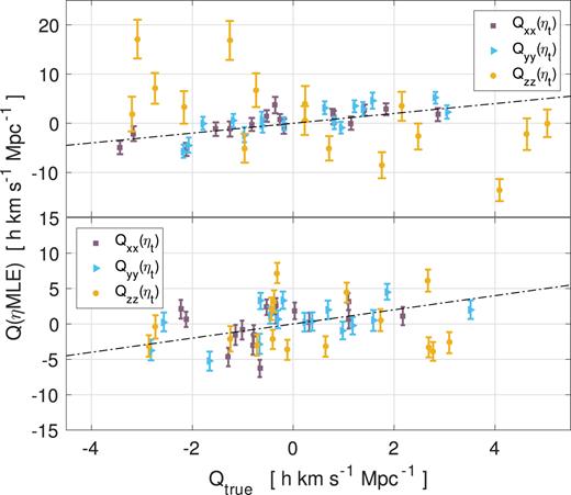
The measurements of the diagonal elements of Q for the half-sky 2MTF mocks using ηMLE. In the upper panel, we set Qzz as an independent component in the MCMC routine. In the bottom panel, Qzz is not independent in the MCMC routine.
