


ABSTRACT
We present the results of the archaeological analysis of the stellar populations of a sample of ∼4000 galaxies observed by the SDSS-IV MaNGA survey using pipe3d. Based on this analysis we extract a sample of ∼150 000 star formation rates (SFRs) and stellar masses that mimic a single cosmological survey covering the redshift range between |$z$| ∼ 0 and |$z$| ∼ 7. We confirm that the star-forming main sequence holds as a tight relation in this range of redshifts, evolving in both the zero-point and slope. This evolution is different for local star-forming (SFGs) and retired (RGs) galaxies, with the latter presenting a stronger evolution in the zero-point and a weaker evolution in the slope. The fraction of RGs decreases rapidly with |$z$|, particularly for RGs at |$z$| ∼ 0. We detect RGs well above |$z$| > 1, although not all of them are progenitors of local RGs. Finally, adopting the required corrections to make the survey complete in mass in a limited volume, we recover the cosmic SFR, stellar-mass density, and average specific SFR histories of the Universe in this wide range of look-back times. Our derivations agree with those reported by various cosmological surveys. We demonstrate that the progenitors of local RGs were more actively forming stars in the past, contributing to most of the cosmic SFR density at |$z$| > 0.5, and to most of the cosmic stellar-mass density at any redshift. They suffer a general quenching in the SFR at z ∼ 0.35. Below this redshift the progenitors of local SFGs dominate the SFR density of the Universe.
1 INTRODUCTION
Galaxies in the Local Universe are the consequence of their cosmological evolution, storing in their morphologies, dynamics, stellar populations, and gas properties the fossil records of the processes that shaped them. There are two main observational approaches to study this evolution: (i) the analysis of the so-called cosmological surveys, i.e. observations of statistically significant and representative samples of galaxies that allow us to characterize the properties [stellar mass, star formation rate (SFR), metallicity, etc.] of the bulk population at different redshift (e.g. Pérez-González et al. 2008) and (ii) the analysis of the fossil records of this evolution in the properties of galaxies observed in the Local Universe, i.e. the so-called archaeological method (e.g. Thomas et al. 2005).
The first approach is by far the more frequently adopted one, being used by many different studies. It has allowed us to understand how galaxies evolve within the colour–magnitude diagram (e.g. Bell et al. 2006), transforming the bulk population between star-forming to more quiescent/RGs (e.g. Wolf et al. 2005); how disc galaxies grow in size, following an inside-out pattern (e.g. Barden et al. 2005; van der Wel et al. 2014); how star formation happens more rapidly in more massive galaxies than in less massive ones (e.g. Pérez-González et al. 2008), what is known as the downsizing paradigm (see e.g. Cowie et al. 1996; Fontanot et al. 2009); what is the general shape of the SFR density in the universe (e.g. Madau & Dickinson 2014; Driver et al. 2018); and how the relation between SFR and integrated stellar mass, mainly comprised in the so-called star-forming main sequence (SFMS), evolves across cosmic times (see e.g. Speagle et al. 2014; Rodríguez-Puebla et al. 2017, and references therein). This approach assumes that galaxies at different redshifts are representative of the same population that evolves with time. By its nature, the approach traces the evolution of galaxies in a statistical way, being unable to trace the evolution of individual galaxies or to connect the exact same population of galaxies at different redshifts without making assumptions of how that population may evolve. On the other hand, it has the major advantage that it directly probes different epochs.
The second approach has been adopted by a smaller number of studies. This approach looks to infer the evolution of individual galaxies by exploring the signatures that this evolution has produced in observational properties of galaxies. In principle, it is possible to recover the star formation and chemical-enrichment histories (SFHs and ChEHs, respectively) of galaxies, and to explore their dynamical evolution, by analysing the spectroscopic properties, morphologies, and kinematics of both their stellar populations and ionized gas. For doing so, it is possible to adopt a particular shape for the SFHs and ChEHs (e.g. Gallazzi et al. 2005; Thomas et al. 2010; Bitsakis et al. 2016; Zibetti et al. 2017), or to infer them in a non-parametric way (e.g. Panter et al. 2007; Vale Asari et al. 2009; Pérez et al. 2013; Ibarra-Medel et al. 2016; García-Benito et al. 2017). This approach is technically complex, prone to large uncertainties based on the adopted procedure (e.g. Sánchez et al. 2016a), the selected templates or stellar libraries (e.g. González Delgado et al. 2014), or even the details on the errors and the assumptions within the analysis (Cid Fernandes et al. 2013, 2014). On the other hand, with this approach it is possible to trace the evolution of individual galaxies without any further assumption and no statistical matching between galaxy subsamples. Adopting this procedure it has been possible to confirm downsizing in galaxies (e.g. Thomas et al. 2005, 2010); to demonstrate that this downsizing happens on local scales (e.g. Pérez et al. 2013; Zibetti et al. 2017); that galaxies form inside-out (e.g. Pérez et al. 2013; Ibarra-Medel et al. 2016); that the SFHs of galaxies are different for different morphological types (e.g. García-Benito et al. 2017); and even to reproduce the cosmic evolution of the SFR density in the Universe (e.g. Panter et al. 2007; López Fernández et al. 2018) or the global metal enrichment (e.g. Asari et al. 2007).
As indicated above, one of the main discoveries of large galaxy surveys was the relation between the SFR and the integrated stellar mass that most galaxies follow, i.e. the SFMS (e.g. Brinchmann et al. 2004; Noeske et al. 2007a; Salim et al. 2007; Renzini & Peng 2015; Sparre et al. 2015). At any redshift, star-forming galaxies (SFGs) present a tight (∼0.2–0.3 dex dispersion) linear correlation between both parameters in the logarithm with a sub-unity slope at low redshifts (e.g. Renzini & Peng 2015; Cano-Díaz et al. 2016). The slope evolves modestly with redshift, being almost constant over cosmological time, and possibly approaching unity at higher redshifts (e.g. Speagle et al. 2014). However, this evolution, although mild, could reflect a change in the overall star formation in galaxies. A unity slope found at high redshift is consistent with an exponential SFH (a shape frequently used to model the SFH of galaxies, e.g. López Fernández et al. 2018), with a time delay that regulates the downsizing. However, a sub-unity slope, typically found in low-redshift studies, implies that the SFH is shallower than an exponential one. On the other hand, the zero-point of the SFMS presents a clear shift towards larger values in the past (e.g. Speagle et al. 2014), following the cosmological evolution of the SFR density in the Universe (e.g. Katsianis, Tescari & Wyithe 2015; Rodríguez-Puebla et al. 2017). This trend may be truncated at very high redshift if the SFR density (per co-moving volume) of the universe, ΨSFR, presents a decline as shown in the so-called Madau plot (e.g. Madau & Dickinson 2014; Driver et al. 2018).
Besides the (star-forming) galaxies along the SFMS, there are galaxies below this sequence, that is, with lower values of SFR for their masses. These galaxies are in a passive/quiescent mode of star formation, and if this mode prevails over time, then we can refer to these galaxies as retired (RGs, hereafter). Analysis based on cosmological surveys show that the fraction of quiescent galaxies increases with cosmic time, with RGs being extremely rare at redshifts higher than ∼2 (e.g. Muzzin et al. 2013; Tomczak et al. 2014; Martis et al. 2016; Pandya et al. 2017).
More recently, Zibetti et al. (2017) and López Fernández et al. (2018)1 adopted an archaeological approach to estimate the cosmic evolution of ψSFR, following the pioneering results by Panter, Heavens & Jimenez (2003) and Heavens et al. (2004). In both cases, they adopted a set of SFH models and compared the observed stellar indices together with multiwavelength photometric data to derive the properties of the stellar populations for galaxies extracted from the CALIFA survey (Sánchez et al. 2012). In the case of Zibetti et al. (2017), the derived cosmic SFH, ΨSFR(|$z$|), presents a similar shape as the one presented by Madau & Dickinson (2014), with a decline at low (|$z$| < 0.5) and high redshifts (z > 4), but with a much broader and shallower peak, centred at lower redshifts (|$z$| ∼ 1–2). The agreement between cosmological surveys and the results of López Fernández et al. (2018) is better, although the peak in the SFR density is slightly broader and shallower than previously reported results.
Following these pioneering studies, we have adopted the archaeological approach for the current study. We explore the evolution of the SFR–M* diagram of both SFGs and RGs across cosmic times based on the analysis of the SFHs derived for ∼4000 galaxies observed by the SDSS-IV MaNGA (Bundy et al. 2015) survey and adequately corrected for volume completeness. Furthermore, we calculate the global SFR and mass density evolution. We address the question of whether the predictions, based on the archaeological approach, are consistent or not with the results from cosmological surveys.
The flow of this article is as follows: In Section 2, we describe the sample and data explored in this study. A summary of the analysis performed on the data is described in Section 3, with details on the derivation of the SFR included in Section 3.1. The main results of the current study are presented in Section 4, including the description of the local SFMS (Section 4.1), and its evolution across cosmic times (Section 4.2). The quantification of this evolution for the different analysed subsamples is explored in Section 4.3. Our estimation of the cosmic SFR density history is included in Section 4.4. The distribution of the stellar-mass density of the universe at different redshifts is described in Section 4.5, and the average specific SFR in Section 4.6. The discussion on the results is presented in Section 5, including a summary of the main caveats on those results in Section 5.1, with details on the effects of mergers included in Section 5.2. The differences between the SFHs of SFGs and RGs are described in Section 5.3. The evolution of the SFMS is discussed in Section 5.5 with details on the turn-over at high mass discussed in Section 5.6. Finally, the implications of the fraction of RGs found along cosmological times are discussed in Section 5.7. The conclusions of our results are presented in Section 6.
In this article, we assume the standard Λ cold dark matter cosmology with the parameters: H0 = 71 km s−1 Mpc−1, ΩM = 0.27, |$\Omega _\Lambda$| = 0.73.
2 SAMPLE AND DATA
We use the observed sample of the Mapping Nearby Galaxies at APO (MaNGA; Bundy et al. 2015) survey collected through June 2017, comprising a total of 4202 galaxies. MaNGA is part of the 4th generation of the Sloan Digital Sky Survey (SDSS-IV; Blanton et al. 2017). The goal of the ongoing MaNGA survey is to observe approximately 10 000 local galaxies; a detailed description of the selection parameters can be found in Bundy et al. (2015), including the main properties of the sample, while a general description of the Survey Design is found in Yan et al. (2016b). The sample was extracted from the NASA-Sloan atlas (NSA; Blanton M. http://www.nsatlas.org). Therefore, all the parameters derived for those galaxies are available (such as effective radius, Sersic indices, multiband photometry, etc.). The MaNGA survey is taking place at the 2.5 m Apache Point Observatory (Gunn et al. 2006). Observations are carried out using a set of 17 different fibre-bundles science integral-field units (IFU; Drory et al. 2015). These IFUs feed two dual channel spectrographs (Smee et al. 2013). Details of the survey spectrophotometric calibration can be found in Yan et al. (2016a). Observations were performed following the strategy described in Law et al. (2015), and reduced by a dedicated pipeline described in Law et al. (2016). These reduced datacubes are internally provided to the collaboration labelled as version 2.2.0 of the data set. This sample includes more than 4200 galaxies at redshift 0.03 < |$z$| < 0.2, covering a wide range of galaxy parameters (e.g. stellar mass, SFR, and morphology), providing a panoramic view of the properties of the population in the Local Universe. For examples of the distribution of galaxies in terms of their redshifts, colours, absolute magnitude and scale lengths, and a comparison with other on-going or recent IFU surveys, see Sánchez et al. (2017).
The MaNGA sample comprises four different subsamples of galaxies, as described by Wake et al. (2017): (i) the primary sample, design to cover at least 1.5 re within the FoV of the different fibre bundles; (ii) the secondary sample, designed to cover at least 2.5 re; (iii) the colour enhanced sample, designed to increase the galaxies within the so-called green-valley; and (iv) a set of different subsamples of ancillary or complementary objects included to make use of fibre bundles unable to be allocated by the previous three categories. According to Wake et al. (2017) it is feasible to perform a volume correction for the two first subsamples (that comprise nearly 90 per cent of the objects) based on the classical Vmax procedure (Schmidt 1968). At the start of this work, no volume correction was available for the currently adopted data set, either in the public domain or distributed within the MaNGA collaboration. Therefore, we calculated our own volume corrections following the prescriptions described in Appendix E. We have performed a set of cross-checks of our volume corrections for the subsample of galaxies for which there is now a publicly available volume correction computed as described by Wake et al. (2017), finding no major differences for galaxies above M* ∼ 109 M⊙. However, below this stellar mass, our volume corrections seem to provide better corrections when comparing the derived luminosity and mass functions with those determined from volume-complete samples. We will discuss our approach in a forthcoming article (Calette et al. in preparation).
3 ANALYSIS
We analyse the datacubes using the pipe3d pipeline (Sánchez et al. 2016b), which is designed to fit the continuum with stellar population models and to measure the nebular emission lines of IFS data. This pipeline is based on the fit3d fitting package (Sánchez et al. 2016a). The current implementation of pipe3d adopts the GSD156 library of simple stellar populations (SSPs Cid Fernandes et al. 2013) that comprises 156 templates covering 39 stellar ages (from 1 Myr to 14.1 Gyr), and 4 metallicities (Z/Z⊙ = 0.2, 0.4, 1, and 1.5).2 These templates have been extensively used within the CALIFA collaboration (e.g. Pérez et al. 2013; González Delgado et al. 2014), and for other surveys (e.g. Ibarra-Medel et al. 2016; Sánchez-Menguiano et al. 2018). Details of the fitting procedure, dust attenuation curve, and uncertainties on the processing of the stellar populations are given in Sánchez et al. (2016a,b).
Prior to any analysis a spatial binning is performed in order to increase the S/N without altering substantially the original shape of the galaxy. For doing so, two criteria are adopted to guide the binning process: (i) a desired S/N for the binned spectra and (ii) a maximum difference in the flux intensity between adjacent spaxels. The first criterion selects an S/N per Å of 50 that corresponds to the limit above which the recovery of the stellar population properties have an uncertainties of ∼10–15 per cent (Sánchez et al. 2016a). The second criterion selects a maximum difference in the flux intensity of a 15 per cent. This corresponds to the typical flux variation along an exponential disc of the average size of our galaxies in a range of 1–2 kpc, and shorter scale lengths for more early-type galaxies.
The application of the two criteria and the spatial binning proceeds in the following way: First, the S/N per Å is derived at each spaxel (spatial pixel) by constructing a narrow-band image centred in ∼5000 Å and comparing the mean flux intensity per Å (signal) with the root-square of the variance within the considered wavelength range (noise). Each spaxel within the datacube with an S/N above the desired goal (S/N > 50) is considered as an independent tessella. Thus, for those spaxels (roughly 10–20 per cent of the total ones Ibarra-Medel et al. 2016), no binning is performed. Those spaxels with an S/N below the desired goal are ordered by their flux intensities. Then the non-binned spaxel with the highest flux intensity is binned with any adjacent one if (i) the adjacent one does not already belong to a previously defined tessella and (ii) the difference in the flux intensity between them is lower than the considered limit. The S/N within the new defined tessella is then re-evaluated by comparing the average flux intensity of the spaxels that comprise the bin with the propagated noise. This process takes into account the co-variance between adjacent spaxels. If the S/N of the binned data is larger than the foreseen goal, then the aggregation of spaxels to this tessella stops, and the process starts with a new spaxel (following the defined flux intensity order). If the S/N of the tessella is still lower than the goal, then the aggregation process is repeated by selecting non-binned adjacent spaxel within the flux intensity limit (using the mean flux intensity within the tessella as the new comparison value). If no spaxel is found fulfilling this criterion the aggregation process stops for this tessella, and a new tessella is created starting from the non-binned spaxel with the highest flux intensity. The procedure is described and discussed in detail in Sánchez et al. (2016b), Ibarra-Medel et al. (2016), and Casado et al. (2017).
As a result of this binning process the original spaxels, with a size of 0.5 arcsec × 0.5 arcsec (e.g. Law et al. 2016), are aggregated in tessellas of variable size. The typical size of the tessellas range between 2 and 5 spaxels in most of the cases, with a few larger ones in the outer regions of the galaxies (e.g. figs 3 and 4 of Ibarra-Medel et al. 2016). Contrary to other binning schemes, the original shape of the galaxy is better preserved by the adopted procedure, not mixing adjacent regions corresponding to clear different structures (e.g. arm/inter-arms). The disadvantage is that it does not provide with an homogenous S/N distribution across the entire FoV and the S/N limit is not reached in all the final bins/voxels. This S/N limit of 50 was selected based on the extensive simulations described in Sánchez et al. (2016a) in order to recover reliably the SFHs and stellar properties in general. For lower S/N those properties are recovered in a less precise but still accurate way. The tessellas with lower S/N are found mostly in the outer regions, where there are still a large number of individual bins. Therefore, averaging the stellar properties (including the SFHs) either radially or integrated across the entire FoV provide uncertainties similar to the ones from individual but larger S/N bins. This was already shown in Ibarra-Medel et al. (2016), and it is discussed in Appendix A. The adopted procedure provides a more accurate SFH than what would be derived from co-adding all the spectra within the FoV into a single one and analysing it, according to recent results (Ibarra-Medel et al. submitted).
Once performed the spatial binning/segmentation, the spectra from spaxels in each tessella are co-added prior to any further analysis. Then, a stellar population fit of the co-added spectra within each spatial bin is computed. The fitting procedure involves two steps: first, the stellar velocity and velocity dispersion are derived together with the average dust attenuation affecting the stellar populations (AV, ssp). Secondly, a multi-SSP linear fitting is performed, using the library described before and adopting the kinematics and dust attenuation derived in the first step. This second step is repeated including perturbations of the original spectrum within its errors; this Monte Carlo procedure provides the best coefficients of the linear fitting and their errors, which are propagated for any further parameters derived for the stellar populations. At the end of this analysis we have a model of the stellar populations for each tessella
Finally, we estimate the stellar population model for each spaxel by re-scaling the best-fitting model within each spatial bin (tessella) to the continuum flux intensity in the corresponding spaxel, following Cid Fernandes et al. (2013) and Sánchez et al. (2016a), a standard procedure in this kind of analysis. This model is used to derive the average stellar properties at each position, including the actual stellar-mass density, light- and mass-weighted average stellar age and metallicity, and the average dust attenuation. In addition, the same parameters as a function of look-back times are derived, which comprise in essence the SFHs and ChEHs of the galaxy at different locations. In this analysis, we followed Sánchez et al. (2016b), but also Cid Fernandes et al. (2013), González Delgado et al. (2016, 2017), and García-Benito et al. (2017). In a similar way as described in Cano-Díaz et al. (2016) and Ibarra-Medel et al. (2016) it is possible to co-add, average or azimuthal average those parameters to estimate their actual (and/or time evolving) integrated, characteristics or radial distributions.
The stellar population model spectra are then subtracted from the original cube to create a gas-pure cube comprising only the ionized gas emission lines (and the noise and residual of the stellar population modelling). Individual emission line fluxes were then measured spaxel by spaxel fitting both a single Gaussian function for each emission line and spectrum, and also making a weighted moment analysis, as described in Sánchez et al. (2016b). For this particular data set, we make use of the flux intensities and equivalent widths of H α and H β (although a total of 52 emission lines are analysed, Sánchez et al. 2016b). All intensities were corrected for dust attenuation. For doing so, the spaxel-to-spaxel H α/H β ratio is used. Assuming a canonical value of 2.86 for this ratio (Osterbrock 1989), and adopting a Cardelli, Clayton & Mathis (1989) extinction law and an RV = 3.1 (i.e. a Milky Way like extinction law), the spatial dust attenuation in the V band (AV, gas) is derived. Finally, using the same extinction law and derived attenuation, the correction for each emission line at each location within the FoV was applied.
After a detailed quality control analysis we restricted the sample to 4101 galaxies, excluding blank fields pointings, very low signal-to-noise targets, galaxies with bright foreground field stars and galaxies at the very edge of the FoV of a MaNGA IFU.
3.1 Star formation rate and stellar mass
The SFR was derived using two different procedures: (i) based on the H α luminosity and (ii) based on the stellar population synthesis analysis. In the first case, we use the H α intensities for all the spaxels with detected ionized gas. The intensities are transformed to luminosities (using the adopted cosmology) and corrected for dust attenuation as indicated before. Then, we apply the Kennicutt (1998) calibration to obtain the spatially resolved distribution of the SFR surface density. A Salpeter initial mass function (IMF) was adopted (Salpeter 1955), the same assumed for the SSP library. We use all the original spaxels irrespective of the origin of the ionization. By doing so, we take into account the PSF wings in the star-forming regions that may present equivalent widths below the cut applied in Sánchez et al. (2017) and Cano-Díaz et al. (2016) (as we will explain in the following sections). On the other hand, we are including in our SF measurement regions that are clearly not ionized by young stars. For SFGs, that contribution is rather low, due to the strong difference in equivalent widths, as already noticed by Catalán-Torrecilla et al. (2015), and therefore the SFR is only marginally affected. However, for the RGs, the ionization comes from other sources, including AGN ionization, post-AGB stars, or rejuvenation in the outer regions (e.g. Sarzi et al. 2010; Papaderos et al. 2013; Singh et al. 2013; Gomes et al. 2016,a,b; Belfiore et al. 2017). Therefore, the H α-based SFR for RGs should be considered as an upper limit, as recently demonstrated by Bitsakis et al. (2018). Hereafter we will refer to this SFR as SFR . We discuss in Appendix B in detail why adopting either integrated SFRs or selecting only those regions that we are totally sure are ionized by local star formation (at the scale of the kpc) do not alter significantly the current analysis.
In the second case we derive the current SFR using the decomposition of the stellar populations in a multi-SSP analysis described above. For each galaxy at each spaxel, it is possible to assign the fraction of light that corresponds to a certain age (by co-adding the fractions of light from different metallicities at the considered age). Taking into account the mass-to-light ratio of each particular SSP and the luminosity in each spaxel it is straightforward to determine the mass that corresponds to stars of a certain age (as described in Sánchez et al. 2017) and at a certain location. Then, by co-adding these masses within the FoV of the datacubes we obtain the integrated mass of stars of a certain age, M*, age. Once we derive this distribution of masses it is possible to integrate from the earliest times up to a certain look-back time and obtain the cumulative mass of the galaxy versus cosmic time (as described in Ibarra-Medel et al. 2016). To do so it is necessary to consider the redshift of the object in order to derive the correct look-back time that is matched against each age within the SSP library. The derivative of this cumulative mass function is, by construction, the SFR at each redshift (or look-back time), thus, the SFH of the galaxy (e.g. González Delgado et al. 2017; García-Benito et al. 2017). In particular, the SFR calculated at the observed redshift is the current one, and we refer to it as SFRssp, 0.
The two estimations of the SFR at |$z$| ∼ 0, SFRH α, and SFRssp, 0, do not follow a one-to-one correspondence, although they present a tight correlation, with an offset of ∼0.11 dex and a dispersion of ∼0.32 dex. These differences are expected due to the different nature of their derivations that are based on different assumptions, as we discuss in detail in Appendix C. We maintain that using either derivation of the SFR at |$z$| ∼ 0 provides similar qualitative results, and that they can be transformed from one to the other adopting a linear relation with a slope near unity. This relation is given in Appendix C.
Contrary to those archaeological methods based on parametric SFHs, our method cannot provide the SFR at any time (SFRt), since it samples the SFH in a discrete way for each galaxy, limited by the ages included within the SSP library (e.g. García-Benito et al. 2017; López Fernández et al. 2018). Our currently adopted SSP library comprise 39 ages. Therefore, we can derive 38 SFRs sampled in the time-steps between each two consecutive ages. Due to the range in redshift of the MaNGA sample each galaxy samples the SFH at slightly different cosmic times, which is particularly important at low redshifts. Some examples of the individual SFHs derived from our inversion methods were presented in previous publications (Ibarra-Medel et al. 2016, figs 2, 3, and 4). To derive these SFHs it was necessary to apply an interpolation to the individual and temporally discrete values and re-sample them to a common look-back time, since, as indicated before, each galaxy samples cosmic time in a different way due to its redshift. Once interpolated, we obtain the median of the SFRs along cosmic time for all galaxies within a considered mass bin. The time range sampled by galaxies of different stellar mass is different due to the strong correlation between this parameter and the redshift in the MaNGA sample (e.g. Bundy et al. 2015). It is beyond the scope of this article to discuss the details of these typical SFHs, and indeed this is not required for the analysis we present here. As a brief summary, it can be said that more massive galaxies have a stronger SFR at earlier times, while less massive galaxies have peak SFRs at lower redshift. This is in agreement with current knowledge of the SFHs in galaxies, known as the downsizing scenario (e.g. Pérez-González et al. 2008; Thomas et al. 2010), and already seen in both the pioneering studies using the fossil record method (Panter et al. 2003, 2007), and in more recent analysis (e.g. Pérez et al. 2013; Ibarra-Medel et al. 2016; García-Benito et al. 2017; López Fernández et al. 2018). We will discuss the shape of the SFHs elsewhere (Ibarra-Medel et al. in preparation).
The main result of our analysis is that for each galaxy we estimate its stellar mass and SFR at 38 look-back times that corresponds to 38 different redshifts for each galaxy. All together our procedure generates a total of 155 838 individual pairs of stellar masses and SFRs that are the result of combining the 38 estimates for each of the 4101 analysed galaxies. This final sample covers a wide redshift range between |$z$| ∼ 0.005 and |$z$| > 8. Although, due the limitations of our adopted procedure, our exploration is reliable only up to z ∼ 3, as we will see later. We correct stellar masses for the mass-loss at the observed time, adopting the prescriptions by Bruzual & Charlot (2003) that depend on the age and metallicity of the population at each redshift.
The SFR derived in this way at the redshift of the object would be the current SFR that we will label as SFRssp. This procedure was used recently by González Delgado et al. (2016) in their exploration of the radial structure of SFR in galaxies. They derive the SFRssp by integrating the stellar mass formed in the last 32 Myr and dividing by this time-scale. This procedure is in essence the same as the one used in the derivation of any SFR calibrator, such as the ones presented by Kennicutt (1998), although in these theoretical calibrators a certain SFH is assumed a priori. Following Speagle et al. (2014), we adopted a time range of 100 Myr in our derivation of the SSPssp, although assuming any range between 10 and 100 Myr would not make any significant difference. A direct comparison between the SFRssp derived using 10, 32, and 100 Myr leads to a systematic offset towards larger SFRs as the time range increases, with increments of 0.06 ± 0.20 dex between 10 and 32 Myr and 0.15 ± 0.18 dex between 32 and 100 Myr. Aside from this offset, there is a clear one-to-one trend; a linear regression between SFRs using any two time ranges yields slopes ranging between 0.82 and 0.97, being always compatible with one. Therefore, as claimed before, adopting any of these time ranges would not change significantly the results.
Finally, we should stress that the integrated mass, SFR, and their evolution obtained from IFS spatially resolved observations are more accurate than those obtained from a single integrated spectrum (the case of single-aperture observations) as shown in Ibarra-Medel et al. (in preparation), who applied both analysis to simulated galaxies.
4 RESULTS
4.1 The local star-forming main sequence
Despite the differences between the H α- and SSP-based SFRs, both present similar general trends when compared with other parameters of the galaxies. In particular, they show a similar trend with the stellar mass. Fig. 1 shows the distribution of the SFRs derived using both estimations versus stellar mass, colour-coded by the EW(H α) averaged across the entire FoV of the datacubes. Two clear trends are seen for galaxies with EW(H α) > 3 Å and galaxies with EW(H α) < 3 Å, for both derivations of the SFR, as already noticed by previous authors (e.g. Cano-Díaz et al. 2016): (i) the SFMS which shows a linear correlation between SFR and M* in logarithmic scales, with a slope slightly lower than one and (ii) the sequence of passive or RGs, which shows a linear correlation only for the SFRH α estimation, and a cloud for the SFRssp.
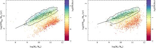
Left-hand panel: Distribution of the SFR derived from the dust corrected H α luminosity versus the integrated stellar mass derived from analysis of the stellar populations for each galaxy in the sample. Right-hand panel: Similar distribution for the SFR derived based on the stellar mass accumulated in the last 100 Myr, based on the stellar population analysis. Each galaxy in each panel is shown as a solid circle coloured based on the EW of H α averaged across the FoV of each datacube. Contours indicate the density for the current SFGs at the redshift where the galaxies were observed, selected as indicated in the text. Outer and inner contours encircle 95 per cent and 25 per cent of the galaxies. Solid black line shows the result from a linear fitting for the SFMS derived at each redshift range.
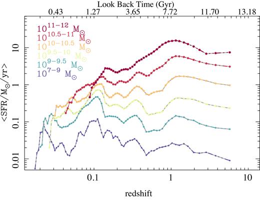
Typical SFHs derived from our analysis of the stellar populations for galaxies in different mass bins. Each line, colour-coded by stellar mass, shows the median SFR at each look-back time for all galaxies within the indicated mass range, interpolated to a common look-back time and re-sampled in a logarithm scale. Solid circles indicate the re-sampled look-back times. Due to the strong relation between the redshift and the mass in the MaNGA sample the sampled time range changes with the stellar mass.
As already discussed by previous authors (e.g. Sánchez et al. 2018), the nature of those two trends is intrinsically different. The former correlation indicates that when galaxies are actively forming stars, the integrated SFR follows a power of the look-back time (not an exponential profile as generally assumed), as discussed by Speagle et al. (2014). On the other hand, the later correlation, evident only for the H α derivation of the SFR, does not reflect precisely a connection between SFR and M*, since actually the dominant ionizing source for galaxies in the RG sequence is not compatible with SF: Cano-Díaz et al. (2016) already have shown that their ionization is located in the so-called LINER-like (or LIER) area of the BPT diagram, being most probably dominated by some source of ionization produced by old-stars (e.g. post-AGBs; Keel 1983; Binette et al. 1994; Stasińska et al. 2008; Binette et al. 2009; Sarzi et al. 2010; Cid Fernandes et al. 2011; Papaderos et al. 2013; Singh et al. 2013; Gomes et al. 2016,a,b; Belfiore et al. 2017). Indeed, its luminosity correlates with M* due to its stellar nature, indicating that they most probably present a characteristic EW(H α) (e.g. Morisset et al. 2016), lower than 3 Å, as predicted by Stasińska et al. (2008) and Cid Fernandes et al. (2011). González Delgado et al. (2017) already showed that when the SFR is not derived from the H α ionized gas, the linear shape disappears, and the RGs are distributed in a cloud shape within the SFR–M* diagram (as appreciated in Fig. 1, right-hand panel).
Ideally for this analysis we would like to select only those regions in galaxies where ionization is compatible with star formation, using classical diagnostic diagrams (e.g. following Sánchez et al. 2017, 2018; Sánchez-Menguiano et al. 2018, and references therein). However, as pointed out by several authors, the contamination by other sources of ionization in the SFR integrated across the entire optical extent of galaxies is rather low in general, due to either the intrinsically low EW(H α) of these non-star-forming ionization regions (e.g. post-AGBs), or the limited extent compared to that of the star-forming regions (e.g. type-II AGNs). Even in the case of type-I AGNs the contamination is rather low, as shown by Catalán-Torrecilla et al. (2015, 2017). We would like to note that in any case removing AGNs from our analysed sample does not affect the results, since the number of AGNs is rather low compared with the bulk population of galaxies (∼3–4 per cent, e.g. Rembold et al. 2017; Sánchez et al. 2018). As a sanity check we have repeated all the analysis presented here using the SFRs derived by selecting only the individual spaxels where ionization is compatible with star formation, following the criteria outlined in Sánchez et al. (2017), see Appendix B. We have found no significant differences. At this point, we prefer to continue with the original procedure and use the integrated quantities since it is more compatible with what it would be done in a cosmological survey based on single aperture spectroscopic data.
Different cuts in EW(H α) have been proposed to select star-forming regions in galaxies. Sánchez et al. (2014) proposed a minimum EW(H α) > 6 Å to select H ii regions in galaxies, while more recently Lacerda et al. (2018) increased that threshold to ∼10 Å for star-forming regions in general. However, when integrating across the optical extent of a galaxy this limit could be relaxed towards lower values. If we consider that an EW(H α) < 3 Å is the limit for ionization due to post-AGB, HOLMES, i.e. evolved stars (e.g. Stasińska et al. 2008), a galaxy that forms stars somewhere within its optical extension, but not everywhere, would have an EW(H α) > 3 Å. Based on this basic assumption Sánchez et al. (2018) classified the galaxies with 3 Å < EW(H α) < 6 Å as green-valley galaxies, somehow between pure SFGs and totally RGs. These galaxies are less than a 10 per cent of the total sample, and their inclusion or exclusion as SFGs do not modify significantly our results. For simplicity, we will include all these galaxies within the subsample of star-forming ones, since indeed they present star formation somewhere within their optical extent.
Both linear regressions are shown in Fig. 1. The differences in the slope reflect the differences found between both estimate of the SFR, described in the previous section. The trend is shallower for SFRssp than for SFRH α. The differences at a fixed stellar mass are even smaller. For example, at the characteristic mass M* ∼ 1010.75 M⊙, the difference is ∼0.12 dex. Thus, we consider that both estimates of the SFR yield similar characterizations of the SFMS at the redshift of the objects once the differences between them are understood. The slopes derived for both esimates of the SFMS are within the range of values reported in the literature for low-redshift samples: 0.77 (Elbaz et al. 2007), 0.65 (Salim et al. 2007), 0.35 ± 0.09 (Chen et al. 2009), 0.63–0.77 (Oliver et al. 2010), ∼1 (Elbaz et al. 2011), 0.67 (Whitaker et al. 2012), 0.71 ± 0.01 (Zahid et al. 2012), 0.63 (Sánchez et al. 2013), 0.76 ± 0.01 (Renzini & Peng 2015), and 0.81 ± 0.02 (Cano-Díaz et al. 2016).
To study the evolution of the SFR on cosmological time-scales we will use not only the local population of SFGs (i.e. SFGs0), as explained above, but also the population of RGs at z ∼ 0 (RGs0). For doing so, we follow Stasińska et al. (2008) and Cid Fernandes et al. (2010), and we select those galaxies for which the average EW(H α) < 3 Å: i.e. the remaining sample once removing the SFGs0. This limit recently has been demonstrated to be a good one to select galaxies and regions in galaxies dominated by diffuse, ionized gas not compatible with star formation (e.g. Sarzi et al. 2010; Papaderos et al. 2013; Singh et al. 2013; Cano-Díaz et al. 2016; Gomes et al. 2016b; Lacerda et al. 2018).
We should indicate that, in essence, this selection criteria between SFGs and RGs is actually selecting galaxies of different morphologies. Fig. 3 shows the distribution of the sSFR with morphological type, colour-coded using the average EW(H α), for the subsample of ∼2500 galaxies for which we have performed a morphological analysis (Sánchez et al. 2018). The figure shows clearly that most of the RGs are early-type galaxies, mostly E/S0s, while most of the SFGs are late-type ones (mostly Sb/Sbc/Sc). Thus, in this article when discussing the properties of RGs we should keep in mind that we are basically discussing the properties of today’s early-type galaxies, and when discussing the properties of SFGs, we refer mostly to late-type galaxies. The figure also illustrates the correspondence between the EW(H α) and the sSFR, described earlier.
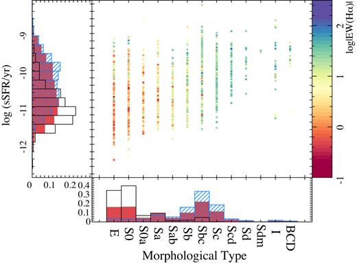
Distribution of specific star formation rates versus the morphological type for the full sample of galaxies, colour-coded by their average EW(H α). The normalized histograms of each parameter for the full sample (solid red), SFGs (hashed light blue), and RGs (open black) are also included.
4.2 Cosmological evolution of the SFR–M* diagram
Having characterized the distribution of galaxies in the SFR–M* diagram (in particular the shape of the SFMS) at the redshift range of the considered sample, and having checked that our estimate of the SFR based on the analysis of the stellar populations is as good as more standard procedures (such as the H α luminosity), we now explore the change of the SFR–M* diagram across cosmic time.
To do so we treat our complete sample of 155 838 individual estimates of M*, t and SFRssp, t as if they comprise a cosmological survey. As explained in Section 3.1, we constructed that synthetic sample by estimating the stellar mass and the SFR at 38 different look-back times for our initial sample of 4101 galaxies based on our multi-SSP fitting procedure. If we consider this synthetic sample as a survey, to explore the evolution with cosmic time we should split the sample in redshift bins that (a) guarantee the required number of objects to do a proper statistical analysis; (b) the resulting subsample in each redshift bin should cover well the SFR–M* diagram; and (c) there should be a reasonably good sampling of redshift to trace the cosmological evolution. Based on these requirements, and considering that we do not have a homogeneous sampling in redshift (due to the discrete nature of the distribution of ages within our SSP library), we split the synthetic sample in nine redshift bins with the following criteria: (i) Each bin must contain at least the same number of galaxies as the original sample (4101). We have shown that this number is large enough to obtain a good description of the distribution along the SFR–M* diagram, and to characterize well the SFMS. (ii) The upper-limit of each redshift bin should be at least Δz = 0.07 away from that of the previous bin. The first criterion is restrictive for high-redshift bins, where our sampling of the temporal domain is more discrete. On the other hand, the second criterion is particularly restrictive at low redshift, where we have a more continuous sampling in the time domain. The selected redshift range corresponds roughly to half the range covered by the original MaNGA sample. Adopting this range ensures we are not dominated by galaxy repetition in each analysed bin, at least at low redshift. We note that neither criteria are particularly restrictive and they do not affect the results so long as enough galaxies are included in each redshift bin to sample parameter space well. Indeed, repeating the same experiment with different numbers of objects we found that with ∼500 galaxies in each redshift bin we can reproduce all the current results if they are distributed along the SFR–M* in a similar way as the original sample (i.e. if they are a representative subsample in this parameter space). However, to ensure a good characterization of the distribution along the SFR–M* diagram, and in particular to study the SFMS across cosmic time, we have been rather conservative in the selection of these redshift bins.
Fig. 4 shows the results of this analysis. For each redshift bin, we present SFRssp, t versus M*, t, labelling each galaxy by its EW(H α) at |$z$| ∼ 0 (the values directly observed, shown in Fig. 1). We use this parameter as a direct observational proxy of their final evolutionary stage (SFGs or RGs) in the Local Universe (as shown in Section 4.1): galaxies with EW(H α) < 3 Å are considered as retired at |$z$| ∼ 0 (the RGs0 sample; reddish in Fig. 4) while galaxies with EW(H α) > 3 Å are considered star-forming at |$z$| ∼ 0 (the SFGs0 sample; blueish in Fig. 4), as explained above. We remind the reader that this cut corresponds well to a cut in sSFR0 at 10−10.8 yr−1, for our currently adopted IMF, based on the correlation between both parameters (e.g. Sánchez et al. 2013; Belfiore et al. 2017).

Distribution of the star formation rate (SFRssp) versus integrated stellar mass (derived from on the analysis of the stellar populations) for each galaxy in the sample at different redshift ranges. For clarity, only those points with an error in the SFR lower than 0.2 dex have been included. The average redshift of each selected range is shown in each panel, and increases from left to right and from top to bottom. Each galaxy in each panel is shown as a solid circle coloured according to the EW of H α measured at |$z$| ∼ 0. Black contours indicate the density for the SFGs in each redshift bin while grey contours indicate the density of RGs, both selected as indicated in the text. Inner and outer contours encircle 25 per cent and 95 per cent of the galaxies, respectively, for each type. Dark-blue solid lines show the linear fit for the SFMS derived at each redshift range (see the text for details). Note that for each particular galaxy within each bin the cut applied to classify it as SFG or RG is different, since it depends on its actual redshift, which explains the overlap between the grey and black contours in the boundary region.
We should note that the first two redshift bins sample times within the redshift range of the original observed sample. Therefore, they do not comprise exactly the same galaxies as the remaining bins: i.e. ‘low’ redshift galaxies (|$z$| < |$z$|max, bin) could be sampled several times in both bins, while ‘high’ redshift galaxies (|$z$| > |$z$|max, bin) are absent by construction. However, this effect is not particularly strong, since most of MaNGA galaxies (∼80 per cent) are located at |$z$| < 0.06 (the upper-redshift of the lower redshift bin), and basically all absent galaxies are RGs0 (due to the MaNGA sample selection). Another caveat to be taken into account is that the diagrams corresponding to the first two redshift bins cannot be easily compared with the distribution shown in Fig. 1, since the number of galaxies is far larger and therefore visual inspection may lead to wrong conclusions.
Despite this caveat we can see a clear evolution in the distribution of galaxies within the SFR–M* diagram with cosmic time. Two main trends arise: (i) The population of RGs at a particular time (RGst) becomes less common at higher redshifts. This is shown in Fig. 4, but it requires quantification, as we will discuss later. (ii) For the SFGs at a particular time (SFGst), the SFR at a fixed mass increases with redshift. Both trends were already known, discovered in studies based on cosmological surveys (e.g. Karim et al. 2011; Whitaker et al. 2012; Speagle et al. 2014). They reflect that galaxies were more actively forming stars individually in the past and that, in general, the cosmic SFR density was larger in the overall (e.g. Lilly et al. 1996; Madau & Shull 1996; Hopkins et al. 2006; Fardal et al. 2007; Madau & Dickinson 2014). The former is particularly true for high- rather than low-mass galaxies, resulting in a steeper SFR–M* relationships at high redshifts. Note that these trends were studied using archaeological methods only once before by López Fernández et al. (2018), and using a much reduced sample of galaxies.
4.2.1 Fractions of retired galaxies at different redshifts
Fig. 5 illustrates the result of this analysis. It shows the histograms of sSFR of the galaxies classified as retired and star-forming at each epoch (red and blue lines, respectively) following the two cuts described above. Each panel corresponds to the different redshift bins described before (i.e. those shown in Fig. 4). According to the first cut (equation 1), both groups should be separated only by a limiting sSFR at each |$z$|. The second cut introduces a mass dependence, and this is why the sSFR histograms of SFGst and RGst have some overlap in each redshift bin. The histograms clearly illustrate the evolution of the fraction of RGst (FRG) to SFGst (1 − FRG) across cosmic time for the complete sample of galaxies. This analysis can be further performed for the subcategories of galaxies classified as star-forming and retired at |$z$| ∼ 0 (SFGs0 and RGs0, respectively), to explore the differences in their evolution.
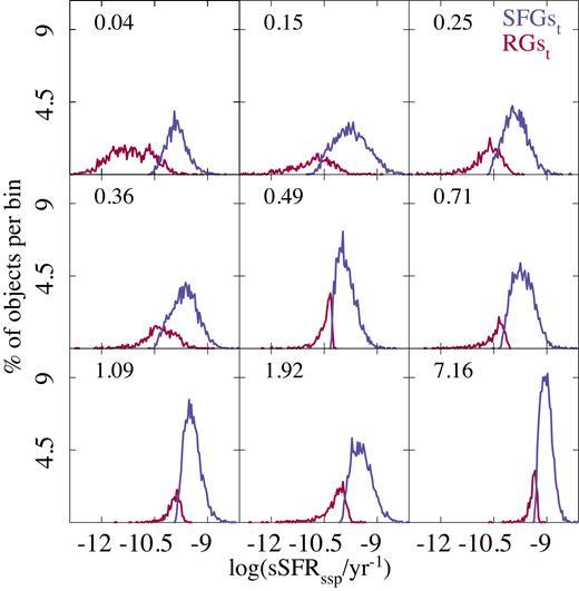
Histogram of the SFRs for the galaxies classified as retired (RGt, red line) or star-forming (SFGst, blue line) in each of the redshift bins shown in Fig. 4, derived from our analysis of the synthetic catalogue described in the text. The mean redshift of each bin is indicated in each panel. The figure illustrates the evolution of the fraction of retired and star-forming galaxies with cosmic time.
Fig. 6 shows the derived distribution of the fraction of RGs as a function of look-back time, tlb, for the full sample of galaxies (black stars), and for the two subsamples defined as SFGs (blue squares) and RGs (red circles) at |$z$| ∼ 0. These values, extracted from the analysis illustrated in Fig. 5, are reported in Table 1, together with the values found at |$z$| ∼ 0 reported in the previous sections for comparison purposes. The reported evolution is now clearly shown in a quantitative way. In general, we find that the fraction of RGst decreases with redshift, although not in a steady way (i.e. there are fluctuations along the main trend). The evolution is consistent with the fraction of RGs0 described in previous sections (∼59 per cent), showing a clear increase in the last 4 Gyr (|$z$| < 0.5).
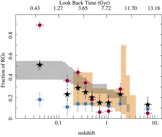
Fraction of RGs as a function of redshift, for all the analysed galaxies (black solid stars), the currently star-forming (blue solid squares), and retired (red solid squares) galaxies, with their corresponding errors (1σ range). The shaded orange regions correspond to estimates of the RG fractions from Muzzin et al. (2013, see the text for details), while the shaded grey regions correspond to the fraction of retired galaxies estimated from Pandya et al. (2017).
Results of the analysis of the SFMS for each redshift bin and galaxy subsample, including (1) the average redshift of each bin; (2) the zero-point and slope of the best-fitting log-linear regression between the SFR and the M* for the SFGs at each redshift, with their corresponding errors; (3) the SFR at a mass of 1010.75 M⊙, with errors corresponding to half the dispersion in the SFMS; and (4) the fraction of retired galaxies. For comparison purposes we include in the two first rows the same parameters derived for galaxies at |$z$| ∼ 0 extracted from the distributions shown in Fig. 1, for both the SFRs derived using the H α flux and the SSP analysis.
| Selection | SFR0 | Slope | SFR10.75 | FRG |
|---|---|---|---|---|
| parameter | log (M⊙ yr−1) | log (M⊙ yr−1) | ||
| SFR | Original sample at z ∼ 0 | |||
| H α | −8.96 ± 0.23 | 0.87 ± 0.02 | 0.32 ± 0.21 | 0.59 |
| SSP | −6.32 ± 0.17 | 0.61 ± 0.02 | 0.28 ± 0.21 | 0.58 |
| z | All galaxies at different redshifts | |||
| 0.04 | −6.47 ± 0.32 | 0.66 ± 0.03 | 0.57 ± 0.21 | 0.51 |
| 0.15 | −5.55 ± 0.30 | 0.55 ± 0.03 | 0.38 ± 0.21 | 0.22 |
| 0.25 | −6.97 ± 0.43 | 0.69 ± 0.04 | 0.42 ± 0.16 | 0.27 |
| 0.36 | −5.78 ± 0.32 | 0.50 ± 0.03 | 0.62 ± 0.16 | 0.27 |
| 0.49 | −9.78 ± 0.22 | 0.98 ± 0.02 | 0.72 ± 0.12 | 0.21 |
| 0.71 | −10.82 ± 0.32 | 1.11 ± 0.03 | 1.10 ± 0.21 | 0.15 |
| 1.09 | −8.39 ± 0.29 | 0.88 ± 0.03 | 1.11 ± 0.13 | 0.15 |
| 1.92 | −8.51 ± 0.27 | 0.90 ± 0.03 | 1.14 ± 0.19 | 0.25 |
| 7.16 | −8.67 ± 0.17 | 0.96 ± 0.02 | 1.62 ± 0.12 | 0.13 |
| z | SFGs0 at different redshifts | |||
| 0.04 | −6.99 ± 0.40 | 0.71 ± 0.04 | 0.67 ± 0.20 | 0.18 |
| 0.15 | −6.73 ± 0.42 | 0.69 ± 0.04 | 0.72 ± 0.19 | 0.11 |
| 0.25 | −8.67 ± 0.27 | 0.87 ± 0.03 | 0.70 ± 0.19 | 0.13 |
| 0.36 | −6.54 ± 0.22 | 0.68 ± 0.02 | 0.75 ± 0.13 | 0.16 |
| 0.48 | −10.67 ± 0.32 | 1.07 ± 0.03 | 0.83 ± 0.18 | 0.15 |
| 0.71 | −11.65 ± 0.24 | 1.19 ± 0.02 | 1.09 ± 0.12 | 0.15 |
| 1.09 | −8.74 ± 0.26 | 0.92 ± 0.03 | 1.13 ± 0.12 | 0.13 |
| 1.92 | −8.85 ± 0.19 | 0.92 ± 0.02 | 1.08 ± 0.17 | 0.16 |
| 7.16 | −8.70 ± 0.21 | 0.96 ± 0.02 | 1.58 ± 0.10 | 0.09 |
| z | RGs0 at different redshifts | |||
| 0.05 | −7.78 ± 0.57 | 0.76 ± 0.06 | 0.37 ± 0.27 | 0.89 |
| 0.15 | −6.17 ± 0.35 | 0.60 ± 0.04 | 0.23 ± 0.17 | 0.36 |
| 0.25 | −7.02 ± 0.23 | 0.68 ± 0.03 | 0.26 ± 0.22 | 0.40 |
| 0.36 | −5.08 ± 0.18 | 0.51 ± 0.02 | 0.43 ± 0.18 | 0.34 |
| 0.49 | −8.16 ± 0.15 | 0.82 ± 0.02 | 0.64 ± 0.12 | 0.19 |
| 0.71 | −8.55 ± 0.27 | 0.90 ± 0.03 | 1.06 ± 0.16 | 0.06 |
| 1.09 | −6.30 ± 0.19 | 0.68 ± 0.02 | 1.04 ± 0.12 | 0.08 |
| 1.92 | −4.77 ± 0.26 | 0.52 ± 0.03 | 0.86 ± 0.15 | 0.28 |
| 7.16 | −7.56 ± 0.20 | 0.85 ± 0.02 | 1.59 ± 0.11 | 0.05 |
Our results are consistent with estimates of the fraction of quiescent/RGs from various cosmological surveys (e.g. Muzzin et al. 2013; Tomczak et al. 2014; Martis et al. 2016; Pandya et al. 2017). In particular, in Fig. 6 we compare our results with those obtained from the COSMOS/UltraVISTA field survey (Muzzin et al. 2013, orange shaded region) and the values reported based on the analysis of the GAMA and CANDELS surveys (grey shaded region Pandya et al. 2017). Muzzin et al. (2013) report the fraction of RGst as a function of mass and |$z$|. To compare with them we weight masses at a given |$z$| with the galaxy stellar-mass function at that |$z$| to obtain the global fractions as a function of |$z$| only. We propagate the errors; the shaded region in the figure corresponds to the regime between ±σ around the mean value within each redshift bin (shown as the size of each box) explored by those authors. For the values reported by Pandya et al. (2017), we adopt the global fractions listed in their table 4. They classified galaxies in three groups based on their distance to the SFMS at a particular redshift. Galaxies with an SFR larger than 1.5σ below the location of the SFMS were classified as star-forming, while galaxies with an SFR lower than 3.5σ were classified as retired. Galaxies between the two regimes were classified as transition objects. This classification is not exactly the same as the one presented here, where we use, in practice, a 2σ threshold below the location of the SFMS to classify galaxies as star-forming or retired. To compare with our results we consider that only 50 per cent of their galaxies classified as transition objects would be classified as RGs, while a 50 per cent would be classified as SFGs. Accordingly, we have combined their two fraction of objects to generate the values shown in Fig. 6, with the lower limit corresponding to their reported fraction of RGs minus 1σ of their reported error, and the upper limit being their reported fraction of RGs plus a 50 per cent of transition objects, in addition to 1σ of their reported error. In general, our results are consistent with those reported by Muzzin et al. (2013) and Pandya et al. (2017). In the first case, the fractions of RGs are always within the regime covered by their fractions, showing even a similar increase at |$z$| ∼ 2. In the second case, our values agree within the errors for the lowest redshift range and at |$z$| ∼ 2. Our fraction of RGs follows a similar decreasing shape with redshift, but in general they are ∼1σ below their reported values for most of the explored redshift regimes.
Going beyond what it was explored by cosmological surveys, we find that the trend of the RG fraction with |$z$| is not universal and is not steady. First, the progenitors of local RGs0 seem to follow the general trend, with a larger fraction of them being SFGs in the past, at least below |$z$| <1.5 (tlb < 8 Gyr). However, for the progenitors of local SFGs0, the fraction of RGst seems to be rather constant with redshift, reflecting that indeed some of them were retired or less active at high redshift. This fraction is ∼15 per cent at any redshift bin. By construction, it is zero at |$z$| ∼ 0. Beyond the nominal error estimated by our procedure, we would be cautious about the significance of any fraction below a 10 per cent, in particular when the defined boundary between SFGs/RGs is near to the location of the SFMS at the considered redshift. Thus, in general we conclude that the fraction of local SFGs0 that fluctuate in an out of the SFMSt is of the order of a 10 per cent at all times. This result cannot be contrasted with cosmological surveys, since by construction, they cannot sample the same galaxies, and trace whether they will become retired or star-forming in the Local Universe. However, they can be compared with the expectations from semi-analytical models. Indeed, Pandya et al. (2017) explored that possibility and reported that 13 per cent of their galaxies classified as SFGs0 and 31 per cent of the ones classified as RGs0 have experienced some kind of rejuvenation in their SFHs since z ∼ 3. Actually, these fractions would be ∼25 per cent for SFGs0 and ∼44 per cent for RGs0, if we consider the fifty-fifty sharing of galaxies classified as transition objects by Pandya et al. (2017) between the two groups.
The second result to highlight is that the fraction of RGst seems to increase slightly at |$z$| ∼ 2 for both the full sample and for that of local RGs only (RGs0). Interestingly, the results from Muzzin et al. (2013) also shows this feature. We should be cautious about this result for two reasons: (i) the last two redshift bins are in a regime where the real redshift or cosmological distance sampled by our archaeological method have significant uncertainties, as we will discuss below and (ii) the boundary between SFGst from RGst at this redshift is closer to the location of the SFMSt than at any other redshift ranges, and therefore some of the galaxies classified as retired could well be SFG ones, particularly at the lower end of the SFMS distribution. However, a visual inspection of Fig. 4 indicates that indeed the fraction of RGs in this redshift bin seems to be enhanced compared to the adjacent redshift bins. In any case, this result is limited by our adopted procedure and the reliability of our fractions at that high redshift, and should be explored in detail prior to drawing a firm conclusion. Thus, the only case in which we could claim that we detect a significant population of RGs at very high redshift is at |$z$| ∼ 2. This result is also shown in Fig. 2, where a drop in the SFR is present at about the same redshift. Further, some of the RGs at this redshift become star-forming again at lower redshifts, indicated as well by the trend in the mean SFH. While we refrain from making a firm conclusion, if these trends in SFH and RG fraction are confirmed, this may indicate that quenching is not a one-way process at this epoch, consistent with the results presented by Pandya et al. (2017) based on their semi-analytical models. Indeed, exploring the individual behaviour of each galaxy in terms of their location within the SFR–M* diagram we see that it is not uncommon for galaxies to become retired and then return to star-forming several times. We will explore in more detail these individual tracks in a companion article (Ibarra-Medel et al. in preparation). So far, we should keep in mind that the average fraction of RGst declines at high redshift, and that decline is dominated by those galaxies defined as retired at z ∼ 0 (RGs0). How this decline depends on other properties of the galaxies, such as stellar mass (or morphology), is an important topic addressed in previous studies (e.g. García-Benito et al. 2017; González Delgado et al. 2017). Clear differences in the average SFHs with redshift shown in Fig. 2 indicate that these properties (e.g. mass) strongly correlate with their evolution. We will explore these correlations in future analysis, now that we have established the validity of our method to explore the evolution of the SFR activity over a wide range of redshift. The possible rise of RGs at |$z$| ∼ 2 should be considered a tentative result at this time. We stress out that although we have detected a possible rise of the fraction of RGs in our analysis, and that this rise seem to be present in at least one cosmological survey (Muzzin et al. 2013), it is possible that this result is a spurious effect of the uncertainties associated with the current adopted method at high redshift.
4.3 Quantifying the evolution of the SFMS
In the previous section, we have described the qualitative evolution of galaxies in the SFR–M* diagram, showing that most of the galaxies are more actively forming stars at higher redshift. In this section, we describe the actual evolution of the SFMS in a more quantitative way.
To characterize the SFMS at each redshift bin, we determine the location of the peak of the density distribution of SFGs in the SFR–M* diagram, shown in Fig. 4, at different masses. This peak corresponds to the mode of the distribution, by definition. This mode was estimated for mass bins of Δlog(M) = 0.075 dex, within a range of masses between 108.75 and 1011 M⊙. Only those mass bins comprising at least a 5 per cent of the galaxies were taken into account. The standard deviation along the mode was adopted as the characteristic width of the SFMS for any redshift and mass bin, and used as errors in the subsequent analysis. Then, for each redshift, we perform a linear regression of the set of points defined by these mass bins and the SFRs defined by the peaks/modes of the distribution. The result of this analysis is presented in Fig. 4, and in Table 1, showing for each redshift bin the zero-point and slope of the linear regression, with their corresponding errors derived based on a Monte Carlo iteration. The analysis was repeated for the two local subsamples of galaxies described before, the SFGs0 and RGs0, to explore if they present different evolution with redshift. The corresponding SFMS for those subsamples have been included in Appendix D, Figs D1 and D2, respectively.
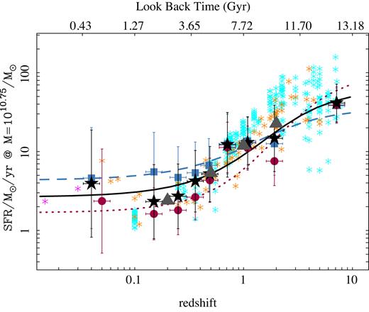
SFR at log(M*) = 10.75 dex versus redshift for each redshift bin shown in Figs 4, D1, and D2 for all the galaxies in the sample (black solid stars), SFGs at |$z$| = 0 (SFGs0; blue solid squares), and RGs at |$z$| = 0 (RGs0; red solid circles). Error bars indicate the dispersion around each derived SFR. Each line represents the best linear fit of SFRs versus look-back time for the complete sample (black solid line), the SFGs0 (blue dashed line), and the RGs0 (red dotted line). Stars represent the values compiled from the literature by Speagle et al. (2014, orange) and Rodríguez-Puebla et al. (2017, cyan). They are based on different direct estimates of the SFMS from cosmological surveys, and therefore they were shifted when necessary to account for the different adopted calibration of the SFR and IMFs. We include the values derived corresponding to the local SFMS by Renzini & Peng (2015) and Cano-Díaz et al. (2016) as magenta stars. Grey solid triangles correspond to values reported by López Fernández et al. (2018) based on a parametric SFH derivation of the galaxies from the CALIFA survey. We also shift their SFR10.75 to correct for the differences in the IMF, when required.
The best-fitting curves are shown in Fig. 7. They illustrate clearly that RGs0 (red dotted line), which were mostly star-forming in the past, show a stronger evolution in SFR than the SFGs0 (blue dashed line). Thus, not only the fraction of RGst increases at lower redshifts, but their global SFR strongly declines too. The average evolution of the full population of galaxies (black solid line) was already noticed by Speagle et al. (2014) and more recently by Rodríguez-Puebla et al. (2017) and López Fernández et al. (2018). We find a good qualitative and quantitative agreement between both results as can be seen in Fig. 7. A comparison between the distribution of characteristic SFR derived from cosmological surveys and best-fitting regression to our data yields a χ2/ν = 0.93 (for Speagle et al. 2014) and 0.95 (for Rodríguez-Puebla et al. 2017), indicating that they are compatible with a significance level higher than p > 0.05. If anything, we find that our estimated SFRs are slightly lower at high redshift (|$z$| > 2) than the ones estimated by cosmological surveys, but in very good agreement with the values reported by López Fernández et al. (2018) using a different archaeological method.
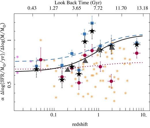
Slope of the SFMS for each redshift bin shown in Figs 4, D1, and D2 for all the galaxies in the sample (black solid stars), the local SFGs (blue solid squares), and the local RGs (red solid circles). The error bars indicate the error in the derived slope. Each line represents the best linear fit of SFR versus look-back time for the complete sample (black solid line), the SFGs0 (blue dashed line), and the RGs0 (red dotted line). The orange stars represent values compiled by Speagle et al. (2014) based on different direct derivations of the SFMS from various cosmological surveys, and magenta stars correspond to the values reported by Sánchez et al. (2013), Renzini & Peng (2015), and Cano-Díaz et al. (2016), respectively. Finally, the grey triangles correspond to values reported by López Fernández et al. (2018) based on a parametric SFH derivation for the galaxies from the CALIFA survey.
4.4 Cosmic star formation history
In previous sections, we have explored how galaxies evolve within the SFR–M* diagram and how the SFMS changes quantitatively with time based on the archaeological analysis of the stellar population of a sample of galaxies at low redshift. Both results are consistent with those reported by cosmological surveys. The basic picture emerging from this analysis is that galaxies were more actively forming stars at earlier times, and that most of the local retired galaxies, RGs0, were once star-forming at higher redshifts. In general, this picture is in agreement with the well-known evolution of the SFR density (per co-moving volume) of the universe (ΨSFR), characterized by the so-called Madau curve (Lilly et al. 1996; Madau & Shull 1996; Madau, Pozzetti & Dickinson 1998). This curve shows a rising of ΨSFR with redshift (and LBT) up to |$z$| ∼ 2–3, and then a possible decline at very high redshift (e.g. Madau & Dickinson 2014; Driver et al. 2018). There remains a large debate about ΨSFR at high redshift because of the discrepancy between different surveys and the large uncertainties due to dust corrections. Indeed, at high redshift most of the SFR density of the universe is inferred via UV light which, to be converted into SFRs, requires quantifying the amount of light obscured by dust. While there is considerable progress in developing empirical constraints on the amount of dust obscuration, the exact shape of the cosmic SFH remains uncertain (see e.g. Reddy & Steidel 2009; Bouwens et al. 2012, 2016; Reddy et al. 2012).
In principle, if our derived individual SFHs based on archaeological methods are a good representation of the real ones, it is possible to recover the ΨSFR at any past cosmic time sampled by our SSP library. It is clear that a detailed comparison between simulated and recovered SFHs is beyond the scope of this article, and will be presented elsewhere (Ibarra-Medel in preparation). We should note that the method has limitations to recover reliable SFHs beyond ages |$t\gtrsim 10$| Gyr, since the SSP templates present small differences at those ages. However, the analysis in previous sections indicates that our estimation of the SFHs is in general compatible with the known evolution of the SFR and mass based on cosmological surveys, at least up to z ∼ 2.
Fig. 9 shows the cosmic SFR density of the universe as a function of look-back time (and redshift), for the full sample of galaxies analysed and the two subsamples of SFGs and RGs at |$z$| ∼ 0, i.e. the SFGs0 and RGs0. The result of all this analysis is included in Table 2. In addition, we include in the figure similar derivations extracted from the literature, based on compilations of different cosmological surveys (e.g. Madau & Dickinson 2014; Driver et al. 2018) or recent archaeological studies (e.g. López Fernández et al. 2018). The estimated ΨSFR(|$z$|) presents the well-known trend, rising from a value of ∼0.01 M⊙ yr−1 Mpc−3 in the nearby universe towards a value ∼10 times larger at |$z$| ∼ 1–2 (tlb ∼ 8 Gyr), and then declining afterwards. Our results agree both qualitatively and quantitatively within the errors with previously reported values extracted from the literature. This agreement is particularly good for the last 8 Gyr. The main difference is found in the peak of the cosmic SFH , which in our case seems to be located at |$z$| ∼ 1, while most cosmological surveys find a peak at |$z$| ∼ 1.5–2.5, particularly for derivations based on far-infrared observations (e.g. Madau & Dickinson 2014). We should be cautious about this result, due to the poorly constrained shape of ΨSFR(|$z$|) beyond |$z$| > 3 for our method, as we will discuss in Section 5.1, Fig. G1, and Appendix G. The bump in the ΨSFR is in general broader than the one reported by Madau & Dickinson (2014), and more similar to the one described by Driver et al. (2018) and López Fernández et al. (2018). Despite these differences, the agreement is remarkable good, particularly in the regime where our results are most reliable, i.e. <8 Gyr.
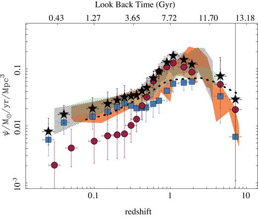
Cosmic evolution of the SFR density derived for all analysed galaxies (black solid stars), SFGs0 (blue solid squares), and RGs0 (red solid squares), with corresponding errors (1σ range). The shadowed regions correspond to the star formation rate densities derived from direct observations based on cosmological surveys compiled by Madau & Dickinson (2014) (the orange solid region corresponds to FIR-derived values while the black hashed region corresponds to FUV-derived values), and Driver et al. (2018) (green hashed region). The black dotted points correspond to the derivation based on archaeological methods presented by López Fernández et al. (2018) based on CALIFA data. When required, literature data has been shifted to account for the different adopted IMFs. The two higher redshift points for our subsamples should be viewed as uncertaint, for reasons described in the text. The average redshift of each subsample in each bin may vary depending on the actual galaxies sampled. This is particularly evident for SFGs and RGs in the lowest redshift bins.
Star formation and stellar-mass density of the universe at different redshift bins, together with the average sSFR, derived from our analysis of the stellar populations of the full sample and the two subsamples of SFGs0 and RGs0. For each redshift we provide the number of galaxies used to derive the parameters, together with the estimated values and the corresponding errors. The listed redshift indicates the average value for the different bins corresponding to each subsample. Those values may change between each subsample, due to the different sampled galaxies.
| z | Ngal | log(Ψ) | log(ρ) | log(sSFR) | Ngal | log(Ψ) | log(ρ) | log(sSFR) | Ngal | log(Ψ) | log(ρ) | log(sSFR) |
|---|---|---|---|---|---|---|---|---|---|---|---|---|
| M⊙ yr−1 Mpc−3 | M⊙ Mpc−3 | yr−1 | M⊙ yr−1 Mpc−3 | M⊙ Mpc−3 | yr−1 | M⊙ yr−1 Mpc−3 | M⊙ Mpc−3 | yr−1 | ||||
| All galaxies | SF galaxies | Retired galaxies | ||||||||||
| 0.03 | 1980 | −2.10 ± 0.29 | 8.79 ± 0.17 | −10.89 ± 0.59 | 1480 | −2.24 ± 0.28 | 8.49 ± 0.15 | −10.73 ± 0.57 | 721 | −2.69 ± 0.27 | 8.47 ± 0.14 | −11.16 ± 0.53 |
| 0.04 | 3694 | −1.80 ± 0.29 | 9.09 ± 0.17 | −10.89 ± 0.59 | 2719 | −1.94 ± 0.28 | 8.79 ± 0.15 | −10.73 ± 0.57 | 1396 | −2.39 ± 0.27 | 8.77 ± 0.14 | −11.16 ± 0.53 |
| 0.10 | 3541 | −1.70 ± 0.23 | 8.99 ± 0.18 | −10.69 ± 0.48 | 2641 | −1.84 ± 0.24 | 8.68 ± 0.16 | −10.51 ± 0.48 | 1319 | −2.27 ± 0.18 | 8.69 ± 0.14 | −10.95 ± 0.36 |
| 0.15 | 3389 | −1.61 ± 0.20 | 8.86 ± 0.18 | −10.47 ± 0.41 | 2564 | −1.75 ± 0.21 | 8.53 ± 0.16 | −10.28 ± 0.43 | 1242 | −2.17 ± 0.13 | 8.58 ± 0.14 | −10.76 ± 0.25 |
| 0.20 | 3065 | −1.55 ± 0.18 | 8.71 ± 0.18 | −10.26 ± 0.38 | 2414 | −1.67 ± 0.19 | 8.43 ± 0.16 | −10.10 ± 0.39 | 1013 | −2.16 ± 0.12 | 8.37 ± 0.14 | −10.53 ± 0.24 |
| 0.25 | 2741 | −1.50 ± 0.17 | 8.48 ± 0.18 | −9.97 ± 0.36 | 2264 | −1.60 ± 0.18 | 8.31 ± 0.16 | −9.91 ± 0.37 | 784 | −2.14 ± 0.12 | 7.96 ± 0.14 | −10.10 ± 0.23 |
| 0.30 | 2843 | −1.48 ± 0.25 | 8.54 ± 0.20 | −10.02 ± 0.52 | 2251 | −1.65 ± 0.26 | 8.32 ± 0.16 | −9.97 ± 0.53 | 919 | −1.99 ± 0.20 | 8.18 ± 0.16 | −10.18 ± 0.41 |
| 0.36 | 2946 | −1.46 ± 0.32 | 8.60 ± 0.22 | −10.06 ± 0.67 | 2238 | −1.69 ± 0.35 | 8.34 ± 0.17 | −10.03 ± 0.72 | 1054 | −1.88 ± 0.25 | 8.33 ± 0.16 | −10.21 ± 0.51 |
| 0.42 | 2993 | −1.39 ± 0.23 | 8.60 ± 0.20 | −10.00 ± 0.48 | 2234 | −1.68 ± 0.26 | 8.30 ± 0.16 | −9.98 ± 0.53 | 1126 | −1.65 ± 0.16 | 8.38 ± 0.16 | −10.03 ± 0.33 |
| 0.49 | 3041 | −1.33 ± 0.16 | 8.61 ± 0.18 | −9.94 ± 0.34 | 2230 | −1.68 ± 0.17 | 8.25 ± 0.15 | −9.93 ± 0.34 | 1199 | −1.49 ± 0.13 | 8.43 ± 0.16 | −9.92 ± 0.26 |
| 0.60 | 3080 | −1.16 ± 0.17 | 8.63 ± 0.20 | −9.80 ± 0.36 | 2209 | −1.61 ± 0.17 | 8.22 ± 0.15 | −9.83 ± 0.35 | 1271 | −1.22 ± 0.13 | 8.52 ± 0.17 | −9.74 ± 0.27 |
| 0.71 | 3119 | −1.05 ± 0.17 | 8.66 ± 0.21 | −9.71 ± 0.38 | 2188 | −1.56 ± 0.17 | 8.19 ± 0.16 | −9.75 ± 0.36 | 1343 | −1.05 ± 0.13 | 8.60 ± 0.18 | −9.65 ± 0.28 |
| 0.90 | 3332 | −0.89 ± 0.17 | 8.69 ± 0.26 | −9.58 ± 0.39 | 2389 | −1.38 ± 0.17 | 8.24 ± 0.17 | −9.62 ± 0.36 | 1350 | −0.96 ± 0.12 | 8.56 ± 0.20 | −9.53 ± 0.27 |
| 1.09 | 3545 | −0.77 ± 0.17 | 8.72 ± 0.30 | −9.49 ± 0.42 | 2591 | −1.26 ± 0.17 | 8.28 ± 0.18 | −9.54 ± 0.37 | 1358 | −0.90 ± 0.12 | 8.52 ± 0.22 | −9.42 ± 0.26 |
| 1.50 | 3584 | −0.84 ± 0.19 | 8.67 ± 0.30 | −9.51 ± 0.45 | 2641 | −1.24 ± 0.19 | 8.32 ± 0.19 | −9.57 ± 0.41 | 1361 | −0.97 ± 0.13 | 8.45 ± 0.22 | −9.42 ± 0.30 |
| 1.92 | 3623 | −0.92 ± 0.21 | 8.62 ± 0.29 | −9.54 ± 0.50 | 2692 | −1.22 ± 0.21 | 8.36 ± 0.21 | −9.59 ± 0.47 | 1365 | −1.06 ± 0.15 | 8.37 ± 0.22 | −9.43 ± 0.35 |
| 4.54 | 2703 | −1.13 ± 0.30 | 8.35 ± 0.53 | −9.47 ± 0.84 | 1899 | −1.48 ± 0.32 | 8.08 ± 0.39 | −9.56 ± 0.83 | 1155 | −1.27 ± 0.26 | 8.11 ± 0.41 | −9.38 ± 0.68 |
| 7.16 | 1783 | −1.54 ± 0.26 | 7.43 ± 0.64 | −8.97 ± 0.74 | 1106 | −2.19 ± 0.27 | 6.81 ± 0.60 | −9.00 ± 0.76 | 945 | −1.71 ± 0.52 | 7.31 ± 0.66 | −9.03 ± 1.46 |
A substantial difference concerning inferences between our archaeological approach and cosmological surveys is that we can trace the SFHs of the same subsample of galaxies without any assumption of how a particular subsample evolves. This was already illustrated in Section 4.2, where we explored the evolution of the SFR–M* diagram for the subsamples of SFGs0 and RGs0. Following the same approach, we include in Fig. 9 the contribution to the SFR density history of both families of galaxies, finding strong differences. The galaxies that are retired in the Local Universe (RGs0), with a halted/quenched SFR in the near universe, present a sharper trend in their cosmic SFH, being on average passive only in the last ∼3.5 Gyr (|$z$| < 0.3). On the contrary, at higher redshifts (particularly between z ∼ 0.5 and z ∼ 2; tlb ∼5–10 Gyr) they are the galaxies that contributed most to the total SFR density of the Universe. The transition between when RGs0’s and SFGs0 dominate the co-moving SFR seems to be a rather fast process that took place in a few Gyr at maximum, in a redshift range between |$z$| ∼ 0.3 and 0.5. However, if we consider the results presented in Section 4.2, not all the RGs0 halt at once, and in some cases individual RGs0 become active and inactive in star formation several times. Therefore, although on average the star formation rapidly diminishes below |$z$| ∼ 0.7 for RGs0, their individual histories may depart considerably from this average behaviour.
The cosmic SFH of the SFGs0 is considerably different. They present a shallower rise of ΨSFR, with an increase of a factor ∼5 from the nearby universe to their peak. The peak is less pronounced, broader, and shifted to slightly higher redshifts (|$z$| ∼ 2). In contrast, the drop at higher redshift (|$z$| > 3) seems to be sharper, indicating that the star formation activity started later in these galaxies than in the retired ones (RGs0). However, we should be cautious about this result due to the large uncertainities at this redshift range. Contrary to the RGs0, SFGs0 do not have a strong drop in SFR at lower redshifts, being in general the galaxies that contribute most to the ΨSFR in the last ∼4 Gyr (|$z$| < 0.4).
We discuss now two aspects of our method of determining ΨSFR(|$z$|). On one hand, if we had selected only one SFR measurement per galaxy and redshift bin, then the correction fraction f given by equation (3) should not have been applied. In this case we should have selected instead either the average SFR along the redshift interval, interpolating our data as a sequence of SFHs, or picked a particular SFR, if we adopt the current approach (i.e. consider our collection of SFR and M* as a cosmological survey). The latter case is illustrated in Fig. H2 in Appendix H. As seen, the differences with Fig. 9 are small.
On the other hand, as indicated before we used only the SFGst subsample for the calculation of ΨSFR(|$z$|). First, these would be the galaxies for which the SFR could be estimated in a cosmological survey. Secondly, below the considered cut in sSFR, the SFRssp becomes very uncertain since it is derived from a very small fraction of young stars (e.g. Bitsakis et al. in preparation). To reflect the effect of this selection we have included in the error budget the differences between using the full sample, without any cut in the sSFR, and using the SFGst to derive the cosmic SFR. We confirm that this selection only affects the derived ΨSFR, t at very high redshift (z > 2), as reflected in the very large error bars in this regime. This is shown in Fig. G1, and discussed in Appendix G.
4.5 Evolution of the cosmic stellar-mass density
Fig. 10, left-hand panel, shows the estimated cosmic stellar-mass density history, ρ*(|$z$|), together with similar derivations extracted from the literature. As in the case of ΨSFR(|$z$|), we find a trend similar to those reported in previous studies based mostly on cosmological surveys. We find a fast rise in ρ* at early epochs, with an increase in the first ∼3–4 Gyr from 107 M⊙ Mpc−3 to near 108.3 M⊙ Mpc−3, followed by a shallower increase in the last ∼9–10 Gyr towards the current value near to 109 M⊙ Mpc−3 (at |$z$| ∼ 0). This characteristic shape is well described by inferences from different cosmological surveys (e.g. Pérez-González et al. 2008; Pozzetti et al. 2010; Ilbert et al. 2013; Muzzin et al. 2013; Madau & Dickinson 2014; Driver et al. 2018).
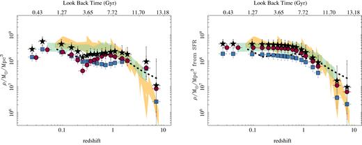
Left-hand panel: Cosmic evolution of the stellar-mass density derived by co-adding the individual stellar masses of each galaxy in each redshift bin corrected by their volume. The density is presented for all the analysed galaxies (black solid stars), the SFGs0 (blue solid squares), and RGs0 (red solid circles), with their corresponding errors (1σ range). The shadowed regions correspond to the stellar-mass densities derived by different compilations presented by Madau & Dickinson (2014) (yellow hashed region), and Driver et al. (2018) (green hashed region). The black dotted points correspond to the derivation presented by López Fernández et al. (2018). As in Fig. 9 shifts are applied in the literature data to take into account the different adopted IMFs, as required. Right-hand panel: Similar plot, but for the stellar-mass densities derived from the integration of the star formation density shown in Fig. 9.
However, the agreement is not as good as it was for the cosmic SFH. Our measurements exhibit a less smooth trend, with a decrease at |$z$| ∼ 0.3 (tlb ∼ 3.5 Gyr) dominated by the contribution of the RGs0. Unless the stellar-mass loss dominates the evolution of the stellar-mass density, which is not the case, this decrease is unphysical. Near this redshift bin we find a considerable decrease in the number of RGs; this may be affecting our statistics (see Table 2). The fact that this drop is not present in the contribution of the SFGs0 supports this suspicion that that the down-turn is an artefact of low-number statistics in this redshift bin. However, we should note that López Fernández et al. (2018) shows a similar drop based on their archaeological analysis of a different sample of galaxies.
The cosmic stellar-mass density histories of the SFGs0 and RGs0 show differences, but not as distinct as the ones shown in the cosmic SFHs, largely because the stellar-mass density is an integral quantity. The RGs0 contribute more to ρ* in the first ∼9 Gyr of the cosmic history of the universe, while in the last ∼4 Gyr both subsamples of SFGs0 and RGs0 have similar stellar-mass densities. The strongest difference happens in the highest redshift bin, at |$z$| ∼ 7, where the contribution of the RGs0 is 10 times larger than that of the SFGs0. However, the errors in this very last redshift bin are large, and therefore the result is not robust.
It seems that our first estimate of the cosmic stellar-mass density is more prone to statistical fluctuations in the sampled number of galaxies. However, by construction it should be most comparable to a cosmological survey, and indeed matches fairly well with the literature results (if we exclude the redshift range between |$z$| ∼ 0.2 and 0.3). Our second estimate is less affected by statistical fluctuations and agrees well at all redshifts with derivations based on cosmological surveys.
4.6 Evolution of the cosmic specific star formation rate
Having derived the cosmic SFR and stellar-mass densities, it is possible to estimate the average sSFR of the universe by dividing these two quantities. This parameter was estimated at each redshift bin and galaxy subsample, and it is listed in Table 2. Fig. 11, left-hand panel, shows the distribution of |$\langle \mathrm{ sSFR}\rangle$| versus cosmic time compared with similar derivations extracted from the literature. In this case we adopt our first estimate of the stellar-mass density, as listed in Table 2 and shown in the left-hand panel of Fig. 10. As in the case of ΨSFR(|$z$|) and ρ*(|$z$|), we find a similar trend between our reported |$\langle \mathrm{ sSFR}\rangle$| and the values reported in the literature. There is a general and steady decrease of |$\langle \mathrm{ sSFR}\rangle$| from the early universe, with values near 10−9 yr−1, to the current time, with values near 10−11 yr−1. There is an offset between our reported |$\langle \mathrm{ sSFR}\rangle$| and those found in the literature from cosmological redshift surveys, while our results agree well at all redshifts with López Fernández et al. (2018). Our values are higher than those using FIR surveys reported by Madau & Dickinson (2014) by about ∼0.1–0.2 dex from 0.1 < |$z$| < 1, and lower at |$z$| > 2. The difference is stronger at high redshift (|$z$| > 2), where ours clearly depart from previously reported results.

Left-hand panel: Cosmic evolution of the average sSFR derived by co-adding the individual sSFR’s of each galaxy corrected by their volume. The |$\langle \mathrm{ sSFR}\rangle$| is presented for all analysed galaxies (black solid stars), SFGs0 (blue solid squares), and RGs0 (red solid squares), with their corresponding errors (1σ range). Shadowed regions and the black dotted line correspond to the same literature results shown in Fig. 9. The blue dash–dotted line shows the best fit to the results by Elbaz et al. (2011). The grey solid line shows the lower limit to the sSFR adopted to select SFGs at each redshift. Right-hand panel: Similar figure when the |$\langle \mathrm{ sSFR}\rangle$| is derived by dividing the star formation density shown in Fig. 9 by the stellar-mass density shown in right-hand panel of Fig. 10.
Following the methodology reported in the previous subsection regarding the analysis of the stellar-mass density, we repeated our estimate of the average sSFR by dividing the SFR density, ΨSFR, shown in Fig. 9, by the stellar-mass density derived from the integration of this very same quantity, ρ*, Ψ(|$z$|), shown in the right-hand panel of Fig. 10. This second estimate of |$\langle \mathrm{ sSFR}\rangle$| is shown in the right-hand panel of Fig. 11. As for the case of ρ*, Ψ(|$z$|), the second estimate has much smoother behaviour with time. There is a steady decrease in |$\langle \mathrm{ sSFR}\rangle$| from the early universe, with the only exception in the highest redshift bin, where there is a drop similar to our initial estimate (Fig. 11, left-hand panel). Agreement with estimates from cosmological surveys is very good except below |$z$| < 0.1 and above |$z$| ∼ 5. In particular, the reported values match well with the best fit reported by Elbaz et al. (2011), with only two values departing from this trend (again, those at the highest and lowest redshift bins). Qualitatively, the trends found for SFGs0 and RGs0 are very similar with this second estimate of |$\langle \mathrm{ sSFR}\rangle$|, although the differences between both subsamples are more clearly highlighted now. In general, the contribution of RGs0 dominates the |$\langle \mathrm{ sSFR}\rangle$| at redshifts beyond |$z$| > 0.5, with a sharp decrease below this redshift (sharper with this second estimate than for the first one). When compared to the contribution of the SFGs0, the trend for the progenitors of local RGs appears delayed at early epochs even though the progenitors of local SFGs have lower values of sSFR at these times. SFS have a shallower evolution below |$z$| < 1, and hence dominate the local average sSFR (as expected by construction of this subsample).
The adopted limit in sSFR to pre-select SFGs at a given redshift (equation 1) has been included in both panels of Fig. 11 (grey line). We see that the average |$\langle \mathrm{ sSFR}\rangle$| is above this limit for most of the considered redshift ranges, in particular for the direct estimate shown in the left-hand panel. As expected, the progenitors of local RGs approach this limit at low redshift, and those that are still forming stars present a lower SFR than the progenitors of local SFGs at the same look-back time.
5 DISCUSSION
We have shown how archaeological methods can be used (i) to trace the evolution of galaxies in the SFR–M* diagram and (ii) to estimate the cosmic SFR and stellar-mass density histories in the Universe. In this section, we discuss the caveats and implications of these results.
5.1 Caveats on the methodology
Prior to any discussion we should mention the main caveats of the current adopted methodology. As extensively explained in Sánchez et al. (2016a,b), the SFHs of galaxies can be recovered only up to a certain limit of reliability, and the derived results are strongly attached to the adopted methodology. The results depend particularly on the adopted SSP template library. In the current analysis, we adopted the GSD156 library (Section 3). This particular library samples time in 39 non-continuous, non-regular ages with almost a logarithmic sampling. The main caveat for this library is that the age of the oldest SSP, 14.13 Gyr, is indeed older than the universe under the assumed cosmology (13.72 Gyr). The reason to include this old SSP is a technical one, since in this way we avoid the oldest stellar population being over represented due to saturation of the sampling and the effects of random noise. Since, due to the adopted procedure, we sample the cosmological times at the look-back times between sampled ages (to derive the SFR one needs to obtain the ΔM* between two consecutive SSPs, separated by Δt), we in fact do not sample ages older than the Universe. However, the measurements in the very last redshift bin shown in Fig. 4, and the two last bins discussed in Section 4.4 and subsequent subsections could be affected in two different ways: (i) the actual sampled look-back time could have large uncertainties and (ii) since the time variable may contain uncertainties, the derivation of the SFR would indeed contain these uncertainties as well. We have tried to determine the uncertainties by repeating the analysis assuming the different possible time ranges Δt, making a random sampling of the time, and associating them to a particular SSP based on their vicinity to the nominal age. Then, we recalculate the time and the SFR considering this new time range. The standard deviation of the distribution of values found using this method with respect to the original value of the SFR has been included in the error budget of the values shown in Figs 9–11, and listed in Table 2. The effect is strong in the very last redshift bins (|$z$| > 3) for the ΨSFR and |$\langle \mathrm{ sSFR}\rangle$| derivations.
The second major caveat regarding our results is the selection of SFGs at different redshifts. We have adopted a cut in the sSFR to perform a first selection of those galaxies that actively form stars at given time. Then, based on the parametrization of the SFMS, we perform a second cut, as described in Section 4.2. These two selections are adopted to identify which galaxies contribute to the ΨSFR at each redshift bin. The first cut is broadly used, and it is the one that affects more the scale of the distributions up to redshift |$z$| ∼ 2–3. However, this first cut does not affect considerably its shape; if no cut in the sSFR is performed we would find the same rising shape in the SFR density, but at slightly larger values than the predictions by cosmological surveys. Beyond this redshift, it is the second selection that affects more the results, shaping the drop in the SFR density at |$z$| > 3. Thus, not performing this second cut, the derived values for the ΨSFR, t would remain almost constant in the last two redshift bins (although they would be clearly within the estimated errors). This is well illustrated in Fig. G1, and discussed in Appendix G. The fact that by doing these two selection cuts we reproduce very well the well-known shape of the ΨSFR(|$z$|), ρ*(|$z$|), and |$\langle \mathrm{ sSFR}\rangle$|(|$z$|) is reassuring. However, due to the uncertainties on both cuts, we should remain cautious about the shape of these distributions at high redshifts.
Finally, the third major caveat concerns the very nature of the procedure adopted here. The stellar population analysis that we perform based on fit3d/pipe3d provides us with the fraction of light that comes from a particular set of stars of a particular age. These light fractions are then transformed to mass-fractions via the M/L ratio of each particular SSP, and finally to masses, considering the luminosity of the galaxy. Therefore, we have assumed that all mass increase in galaxies from one age to another is due to star formation in situ. This argument neglects the mass growth by galaxy mergers, either major or minor. We know that wet mergers had a strong influence at early epochs, in particular beyond tlb >8 Gyr (e.g. Papovich et al. 2005), where these mergers induce strong star formation events. However, these events happen in the primary galaxy and can be considered as in situ star formation. At later epochs, the merger rate is much lower (e.g. Jogee et al. 2009), although for massive early-type galaxies it is expected that they have suffered at least one major dry-merger since |$z$| ∼ 0.7 to the present time (e.g. Bell et al. 2006).
However, mergers do not alter the shape of ΨSFR(|$z$|), ρ*(|$z$|), and |$\langle \mathrm{ sSFR}\rangle$| as a function of |$z$| based on our procedure. The reason for that is the very nature of the calculation described above. What we determine with the archaeological method is the mass fraction of stars of a certain age. In a dry merger, the global stellar mass is increased. However, if both galaxies had a similar SFH, i.e. they have a similar distribution of stars per age, then the combined SFH would not be affected. On the other hand, if they have different SFHs, the combined SFH would be a mix of both of them. If all galaxies suffer similar merging histories, then the general shape of the explored parameters would not change significantly. This is illustrated in Fig. 12 where the cosmic SFH is shown for a set of simulated galaxies that are the result of a 1:1 merger between galaxies following the evolution found for SFGs0 and for RGs0, respectively. The resulting ΨSFR(|$z$|) follows a shape in between the one found for both subsamples of galaxies, having the same qualitative properties as the one found for the full sample: a smooth rising from the current time to |$z$| ∼ 1–2, with a broad peak, and sharp decline at |$z$| > 3 (again noting that derivations beyond that redshift are uncertaint due to the limitations of the adopted methodology). Thus, dry mergers (or any merger that does not result in an increase in the SFR) by themselves would not affect our calculations.
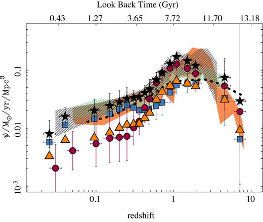
Cosmic evolution of the SFR density derived for a simulated set of galaxies that result from 1–1 mergers between pairs of star-forming or retired galaxies that maintain the SFH of their progenitors (orange triangles). All the other symbols included in the figure are the same as the one shown in Fig. 9.
In addition to these three major caveats, we should keep in mind that our results maybe strongly affected by the methodology of the archaeological procedure adopted here, by its implementation in pipe3d, and by the selection of the SSP library. We aim to narrow-down their effects in future work by performing a detailed analysis of N-body + hydrodynamical simulations (Ibarra-Medel et al. in preparation).
5.2 Merging rate effects on ρ*(|$z$|)
In the previous subsection we discussed the effects of mergers in our calculations. We found that they should not affect significantly the derivation of ΨSFR(|$z$|), however, they should affect somehow the integrated stellar-mass density. As shown in Section 4.5, we found differences between the direct estimates of ρ*(|$z$|), based on co-adding the volume-corrected stellar masses of galaxies sampled at different redshifts (Fig. 10, left-hand panel), and the estimates based on the integration of ΨSFR(|$z$|) over time (Fig. 10, right-hand panel). Some of these differences are indeed due to sampling problems at particular redshifts. However, another possible difference could be due to the contribution of mergers that would not affect the fraction of stars at different ages but could affect the total amount of mass. Actually, we found a clear deviation between our derived stellar-mass density integrating the SFR at high redshift when compared to cosmological surveys (Fig. 10). The deviations in the two highest redshift bins are uncertain, however the trend starts at lower redshift (|$z$| > 1). Thus, although we are cautious about deriving a quantitative estimates from our current analysis, we consider that a feasible explanation for these differences could be the contribution of mergers at high redshift.
5.3 The SFHs of star-forming and retired galaxies
Despite the caveats indicated before, there is a clear result that emerges from our analysis: the galaxies that dominate the SFR budget in the Local Universe are not the ones that dominated at higher redshifts. Most of these later galaxies are now RGs. They dominated ΨSFR at |$z$| >0.5 and then had a sharp drop/quenching of their star formation activity below |$z$| < 0.3. This drop was general, although as we have seen in Section 4, a fraction of these galaxies retired at earlier epochs (|$z$| ∼ 2) and then re-started their star formation activity more recently (|$z$| ∼ 1−2). This switch-off in the star formation activity is clearly connected with the present-day morphology of these galaxies, since, as we indicated in Section 4.1, most of them are ellipticals and S0, which is a well-established result (e.g. Blanton et al. 2005). This change in the SFH with morphology has been recently described by García-Benito et al. (2017), González Delgado et al. (2017), and López Fernández et al. (2018) based on fossil record procedures applied to IFS data. On the other hand, there is also a dependence on stellar mass that we have not explored fully in the current study. In earlier studies by Heavens et al. (2004) and Panter et al. (2007), they showed that more massive galaxies had sharper, more peaked SFHs, and as mass decreases, the SFHs becomes smoother. This result is similar to the one recently presented by García-Benito et al. (2017). Therefore, galaxies of different masses present also different contributions to the global cosmic SFH, ΨSFR(|$z$|). Our current result does not discriminate between stellar mass and or morphology, at least directly. Therefore, we cannot yet determine which is the dominant factor. However, it is clear that local RGs suffered a sharp down-turn in their SFR ∼4 Gyr ago.
More recently, López Fernández et al. (2018), making use of the spatial information provided by the IFS data of the CALIFA survey showed that the central regions of galaxies contribute to the global ΨSFR(|$z$|) with a sharp, peaky, shape similar to that of the early-type or massive galaxies. In contrast, the contribution of the outer regions is shallower, less peaky, similar to that of the late-type or less massive galaxies. Compared to our results, the central regions of galaxies behave like the progenitors of local RGs (RGs0), while the outer regions behave like the progenitors of local SFGs (SFGs0). This fits with our current understanding of galaxy evolution, since we consider that in those galaxies were star formation was starting to halt, this quenching happens from the inside-out, being stronger in more massive and earlier-type galaxies. There is different evidence for this process, such as the direct observation of a drop in the sSFR in the centre of these galaxies (e.g. González Delgado et al. 2016; Belfiore et al. 2017; Sánchez et al. 2018), connected with a drop in the gas content (e.g. Sánchez et al. 2018), and even the flattening or drop of the abundance gradient in the central regions of galaxies (e.g. Sánchez et al. 2014; Belfiore, Maiolino & Bothwell 2016; Sánchez-Menguiano et al. 2016, 2018). The inside-out quenching process has also been seen in cosmological simulations of galaxy evolution (Tacchella et al. 2016; Avila-Reese et al. 2018) and observed at high redshift (e.g. Tacchella et al. 2015). Therefore, the picture that emerges is that SFR was quenched from the inside-out, being connected with the growth of the bulge. For early-type spirals, like Sa and Sb, this quenching is still underway. However, for more early-type galaxies, like S0 and ellipticals, the quenching happens earlier such that these galaxies dominate the budget of RGs in the Local Universe. In summary, there is a mass-grow downsizing and a quenching downsizing, and both seem to present an inside-out pattern and a dependence with morphology.
5.4 The shape of the cosmic SFR density at high redshift
Different cosmological surveys report slightly different shapes for ΨSFR, t beyond z ∼ 1–2, as it can be appreciated in Fig. 9. In general, surveys based on FIR observations estimate larger SFRs, and a less sharp drop in the cosmic SFR than observations involving rest-frame FUV observations (e.g. Madau & Dickinson 2014; Driver et al. 2018). In some cases there is no clear drop, with ΨSFR, t showing a flat distribution or values more consistent with a plateau at this redshift range (e.g. McLure et al. 2018).
Our results in this regards should be taken with care, for the reasons described in this article, and discussed in Section 5.1. In particular, the definition of SFGs and RGs in the highest redshift bins is critical. As shown in Appendix G the inclusion in the computation of the cosmic SFR of the RGst changes dramatically its shape at high redshift, flattening it.
The galaxies that we classify as retired at high redshifts are only slightly below the SFMS (see Fig. 4). We could speculate that these are galaxies at the end of their starburst phase, emitting then mainly in the FIR (sub/millimetric wavelengths at |$z$| ∼ 0) due to the large amount of accumulated dust. Since the redshift determination of submillimetric/dusty SFGs is not very accurate, the cosmological surveys from which cosmic SFR densities are calculated, might be missing the contribution of this population at |$z\gtrsim 4$|. The fossil record method is not affected by this issue. However, as discussed in this paper, our uncertainties at this cosmological times are too large to make any clear claim in this regard.
5.5 The evolution of the SFMS
Our results confirm previous findings indicating that the SFMS is a tight relation, with a very low scatter over a wide range of redshifts (e.g. Brinchmann et al. 2004; Salim et al. 2007; Sánchez et al. 2013; Catalán-Torrecilla et al. 2015; Cano-Díaz et al. 2016; González Delgado et al. 2016). We also confirm that this relation evolves strongly with redshift, both in scale (zero-point) and shape (slope), in agreement with Speagle et al. (2014) and Chiosi et al. (2017). The evolution of the SFMS has been reported in several studies (e.g. Elbaz et al. 2007; Noeske et al. 2007b; Salim et al. 2007; Schiminovich et al. 2007; Pannella et al. 2009; Whitaker et al. 2012; López Fernández et al. 2018). However, the nature of that evolution, either physical or related to observational biases, was questioned due to (i) the differences in the selection of different samples at different redshifts and (ii) the different observational techniques applied to derive the relevant parameters. Therefore, in many cases the homogenization of the data set involved different corrections that may affect the results (see for a discussion Speagle et al. 2014). Our study shows this evolution for the same sample of galaxies, where the involved parameters are derived using the same techniques, thus confirming its physical origin.
Due to the nature of the analysis, this is one of the few studies where we can compare the evolution of the SFMS between local populations of SFGs and RGs, SFGs0, and RGs0, respectively. Indeed, although we find a similar qualitative trend between both subsamples, the detailed evolution seems to be different. SFGs0 show a shallower evolution in amplitude, while RGs0 show a shallower evolution in slope in the SFMS relation. In other words, SFGs0 have a larger average SFR (by a factor ∼2) at low redshift relative to RGs0. However, at high-redshift RGs0 have similar amounts of star formation per unit mass. If star formation happens following the SFMS that is present at high redshift, when both subsamples share this relationship, then those galaxies that are retired in the Local Universe have become less and less active, in particular in the last ∼4 Gyr. However, SFGs0 also form less stars at the same mass than their progenitors at high redshift.
If quenching happens inside-out, as described in the previous section, a natural explanation would be that certain regions of galaxies that still form stars follow the same basic rules while other regions are already quenched. The fact that there is an almost universal spatial resolved SFMS of star-forming regions (e.g. Sánchez et al. 2013; Cano-Díaz et al. 2016; Hsieh et al. 2017), with a mild dependence on the morphological properties of galaxies (e.g. González Delgado et al. 2017, Cano-Diaz et al. in preparation), supports this conclusion. In future studies, we will try to explore the spatially resolved SFMS along cosmological times using the currently adopted procedures to confirm this hypothesis.
5.6 Turnover mass of the SFMS
Different authors have reported that the SFMS has a turnover mass at which the relation deviates from linearity, dropping towards lower SFRs at high masses. This turnover mass has been reported both in the Local Universe (e.g. Catalán-Torrecilla et al. 2015), and at different redshifts (e.g. Lee et al. 2015; Tomczak et al. 2016), observed with many different surveys. The mass at which the SFR drops seems to increase with the redshift. Recent cosmological hydrodynamical simulations of galaxy formation, such as Illustris (Nelson et al. 2015), reproduce this result that the SFR seems to be weaker at higher redshifts and at larger stellar masses (Sparre et al. 2015). This has been recently compared with observations by López Fernández et al. (2018).
We cannot reproduce this drop in the SFR at high masses as shown by previous studies. This could be a consequence of the detailed adopted method to select SFGs at different redshift ranges in our study, involving (i) a cut in the sSFR (that evolves with redshift) and (ii) excluding those galaxies that deviate significantly from the derived SFMS. Indeed, a visual exploration of the distributions of points along the M*–SFR diagram in several redshift bins (Fig. 4) shows that most of the galaxies that deviate from the SFMS are located in the high-mass regime (although it is not a general trend, with a counter example at |$z$| ∼ 0.7). If we had considered them as actively forming stars they would have traced a deviation or drop as the one described by previous studies.
5.7 Fraction of retired galaxies
Different galaxy surveys at high redshift have shown that there are already passive galaxies even at z ∼ 2 (Cimatti et al. 2004; Glazebrook et al. 2004; Muzzin et al. 2013; Pandya et al. 2017). The red-sequence is well established at z ∼ 0.7–1 (Bell et al. 2004; Wuyts et al. 2011), although the fraction of galaxies that populate this sequence is lower than the one found in the Local Universe. We find indeed RGst at any redshift bin from our analysis (Fig. 4), even at z ∼ 2. However, its fraction decreases very quickly with redshift (Fig. 6) with a clear increase at |$z$| < 0.5. Our results are consistent and in some cases agree within the errors with the trends and values reported from cosmological surveys, as we have shown in Section 4.2. We also have found that the transition between SFGs and RGs does not seem to be a single event or a one-way process. A fraction of galaxies retired at high-|$z$| become active at lower redshifts, to be quenched later on. This result is not totally new, since Pandya et al. (2017) already predicted, based on semi-analytical simulations that between a 13 per cent and a 31 per cent of galaxies have experienced rejuvenation events since |$z$| ∼ 3. We will explore that possibility in future analysis, trying to trace the evolution of single objects along the SFR–M* diagram.
Finally, our result disagrees somewhat with those recently presented by López Fernández et al. (2018). Since this is the most recent result based on an archaeological analysis of similar data to the one presented here it is worthy to compare results in more detail. They found almost no RGst beyond |$z$| > 0.5. Those authors speculate that the progenitors of current early-type, mostly RGs, are not those RGs found by cosmological surveys at high redshift, since most of the early-type galaxies at |$z$| ∼ 0 were actively forming stars at high redshift. Our results agree somewhat with this interpretation, since we find that the population of RGs0 were mostly actively forming stars at high redshift (∼80 per cent of them at |$z$| ∼ 2). However, a fraction of them were already RGs at high redshift (∼10–20 per cent). Thus, a fraction of the RGs discovered by cosmological surveys at high redshift are indeed the progenitors of RGs observed in the Local Universe, but not of all of them. The main discrepancy with the results by López Fernández et al. (2018) is that they found basically no RGs beyond |$z$| > 0.5, a result that indeed also disagrees with the results by direct observations based on cosmological surveys (e.g. Muzzin et al. 2013; Pandya et al. 2017).
There are three main reasons that could explain the differences found between our results and the ones presented by López Fernández et al. (2018). First, they used a different sample with fewer galaxies, which may limit the fraction of detected RGs at high redshift, in particular in the regime of very massive galaxies. Some authors (e.g. Toft et al. 2012; Belli et al. 2017) have shown that RGst at high redshift are already very massive objects, with stellar masses between 1010.5−11 M⊙. Thus, they would be most probably the progenitors of galaxies at the edge or not sampled by the CALIFA survey, but maybe sampled by larger surveys, as used here. Secondly, they adopted a parametric SFH to model their data. On one hand, the analytic SFH laws, as the exp-τ, present a smoothly declining SFR after a peak, biasing the inferences in some cases to a smooth and late passage towards the retired regime, in such a way that the fraction of RGs becomes negligible at high redshifts. Some quenching processes in reality can be much faster than the limits imposed by an exponential decline, thereby producing RGs at high redshift. On the other hand, according to these analytical laws, once retired, a galaxy cannot become active at a more recent cosmic time. We have seen that in some cases RGst at a certain look-back time could present a rejuvenation and become active in more recent times. This result is in agreement with several results reported in the literature: (i) blue colours and high SFRs in a fraction of local isolated ellipticals (Lacerna et al. 2016, and more references therein); (ii) weak star-forming, spiral-like, structures found in bona-fide elliptical galaxies in the Local Universe (e.g. Gomes et al. 2016a); and (iii) star formation activity reported in these galaxies based on the combination of near-UV, SDSS r, and mid-IR colour studies (e.g. Gil de Paz et al. 2007; Kaviraj et al. 2007; Ko et al. 2014). Even more, it agrees with the presence of a fraction of RGs at |$z$| ∼ 2 found by cosmological surveys (e.g. Muzzin et al. 2013).
Finally, López Fernández et al. (2018) are sampling galaxies up to larger galactocentric distances, since almost all galaxies are sampled up to 2.5 Re while only a fraction of them are sampled by the MaNGA observations up to these radii. In principle, since the MaNGA FoV does not guarantee that we cover the outer regions of galaxies for all the galaxies, it is possible that our results are biased to tracing more the evolution of the inner regions. This would require an aperture correction to estimate that effect. However, a direct comparison between the integrated stellar masses derived within the MaNGA FoV by pipe3d and those listed in the NSA catalogue do not show any significant aperture effect in our data. Therefore, this should not be the source of discrepancy.
In summary, we should recall that our results fit better with expectations from cosmological surveys. Of the three reasons, the second is the one that could explain the differences in the more natural way. However, the only way to be totally sure that this is the case it is to repeat the current analysis over the data set analysed by López Fernández et al. (2018) and compare with the results. This analysis, that it is clearly beyond the current study, will be presented in a forthcoming article (Sánchez et al. in preparation).
6 CONCLUSIONS
In this study, we explore statistically the evolution of galaxies in the SFR–M* diagram across cosmic time adopting the archaeological approach to follow the stellar population of ∼4000 galaxies in the Local Universe observed by the MaNGA survey. The main conclusions of this analysis are as follows:
We confirm that the SFMS holds as a tight relation between the SFR and the stellar masses over a wide range of look-back times, from the Local Universe to z ∼ 7. The SFMS evolves strongly in its zero-point, illustrating that galaxies form stars in a more active way in the past, and in slope (from ≈0.7 at |$z$| ∼ 0 to ≈1 at |$z$| > 0.5), reflecting that even SFGs are becoming less active in the more massive range in recent times. This evolution is different for the local populations of SFGs and RGs, with the latter presenting a stronger evolution in the zero-point, and a weaker evolution in the slope.
The fraction of RGs decreases rapidly with increasing redshift, in particular for the local population of RGs, rising fast at low redshift (|$z$| < 0.5). However, we are able to detect RGs over a wide range of redshifts up to |$z$| ∼ 2. A fraction of those RGs become active again at lower redshift, although most of them, in particular the more massive ones, end as RGs in the Local Universe.
We are able to recover the cosmic SFR and stellar-mass density histories over a wide range of look-back times, with good precision up to |$z$| ∼ 2. Our results agree qualitatively with the distributions found in studies from different cosmological surveys in all of the explored redshift range, and quantitatively at least for the last 8 Gyr.
The contribution of the local SFGs and RGs to star formation and mass densities is significantly different, with the local RGs being very active in the past, contributing to most of the ΨSFR and |$\langle \mathrm{ sSFR}\rangle$| of the Universe at |$z$| > 0.5, and to most of the ρ* at any redshift. On the other hand, local SFGs dominate the SFR density in the universe in recent times, |$z$| < 0.2, while RGs present a general halting/quenching in their star formation between z ∼ 0.2 and 0.5.
Our results all together indicate that the quenching of the star formation in galaxies is strongly related to their morphology and mass, since most of the currently RGs are indeed early-type massive galaxies. If the quenching happens inside-out, as supported by recent results, then bulge growth in combination with other processes (like gas starvation in dense environments) should be strongly connected with this quenching process. We will address this hypothesis in future studies by exploring the evolution of the SFR at different galactocentric regimes, making use of our spatial resolved information, now that we have confirmed that the integrated properties of star formation and stellar mass match reasonably well with the results found from cosmological surveys on the co-moving SFR and stellar-mass density evolution.
ACKNOWLEDGEMENTS
We would like to thank the referee for his/her comments and suggestions.
We thank the CONACyT programs CB-285080 and DGAPA IA101217 grants for their support to this project. The data products presented in this paper benefited from support and resources from the HPC cluster Atocatl at IA-UNAM.
We thank R. Gonzalez-Delgado, R. López Fernández, R. Cid Fernandes, and E. Lacerda for their pioneering work on this kind of studies, for the generous discussions and the enlightening ideas.
Funding for the SDSS-IV has been provided by the Alfred P. Sloan Foundation, the U.S. Department of Energy Office of Science, and the Participating Institutions. SDSS-IV acknowledges support and resources from the Center for High-Performance Computing at the University of Utah. The SDSS web site is www.sdss.org.
SDSS-IV is managed by the Astrophysical Research Consortium for the Participating Institutions of the SDSS Collaboration including the Brazilian Participation Group, the Carnegie Institution for Science, Carnegie Mellon University, the Chilean Participation Group, the French Participation Group, Harvard-Smithsonian Center for Astrophysics, Instituto de Astrofísica de Canarias, The Johns Hopkins University, Kavli Institute for the Physics and Mathematics of the Universe (IPMU)/University of Tokyo, Lawrence Berkeley National Laboratory, Leibniz Institut für Astrophysik Potsdam (AIP), Max-Planck-Institut für Astronomie (MPIA Heidelberg), Max-Planck-Institut für Astrophysik (MPA Garching), Max-Planck-Institut für Extraterrestrische Physik (MPE), National Astronomical Observatories of China, New Mexico State University, New York University, University of Notre Dame, Observatário Nacional/MCTI, The Ohio State University, Pennsylvania State University, Shanghai Astronomical Observatory, United Kingdom Participation Group, Universidad Nacional Autónoma de México, University of Arizona, University of Colorado Boulder, University of Oxford, University of Portsmouth, University of Utah, University of Virginia, University of Washington, University of Wisconsin, Vanderbilt University, and Yale University.
Footnotes
Details of the actual ages are given in https://data.sdss.org/datamodel/files/MANGA_PIPE3D/MANGADRP_VER/PIPE3D_VER/PLATE/manga.Pipe3D.cube.html
REFERENCES
APPENDIX A: EXAMPLES OF THE SPATIALLY BINNING SCHEME
The binning scheme adopted in pipe3d was described in detail in Sánchez et al. (2016b). It aims to increase the S/N above a certain selected value, but to preserve as much as possible the shape of the original distribution of the light within the galaxy. For this reason, the procedure adopts two criteria to group adjacent spaxels. The first one is just an S/N threshold or limit. If the original spaxel already has an S/N above that goal one, the bin/tessella comprises that original spaxel only. If not, it co-adds adjacent spaxels trying to reach the S/N limit, taking into account the covariance between adjacent spaxels in the S/N analysis. However, contrary to other binning schemes, as a second and more restrictive criterion, it forces the adjacent spaxels to have similar flux intensities in the considered wavelength range. In other words, it does not allow adjacent spaxels of very different flux intensities to be co-added, within a defined fractional difference between considered fluxes. When no adjacent spaxels are found fulfilling this criterion, the aggregation process stops. For this reason this binning scheme preserves better the original shape of the observed galaxy. However, it does not guarantee that the foreseen S/N goal is reached, what it is particularly true for the outer regions of galaxies. Importantly, this method is guaranteed that the areas clearly dominated by sky-noise are well separated from the rest of the tessellas.
This is well illustrated in Figs A1 and A2 where it is shown the S/N distributions prior and after performing the segmentation/binning scheme along the FoV of two galaxies selected randomly from the sample. It is clear the goal S/N (50) is only reached, after binning, for the very central regions (∼15–25 per cent of the tessellas). In general, the S/N is larger than 10–20 for most of the considered tessellas. Those tessellas corresponding to sky-dominated areas are much larger, irregulars, and clearly different than the remaining ones. They were excluded from the analysis by an intensity and S/N cut. The effect of the binning can be quantified by the cumulative functions of the signal-to-noise ratio per spaxel and spatial bin shown in Fig. A3. As indicated before the goal S/N is not reached in all the tessellas after the binning procedure, however, the S/N is clearly increased, both spaxel-wise and within each tessella. For the original spaxels a 20 per cent have an S/N below 7, while for the binned spaxels this percentage corresponds to the double of the S/N. On the other hand, for the individual tessellas this percentage corresponds to S/N of ∼25, and performing a radial bin as the one shown in the upper-right panel of Figs A1 and A2, it corresponds to an S/N of ∼75. Finally, for the integrated spectra through the entire FoV, it corresponds to an S/N ∼ 100. Consistently, only a 20 per cent of the original spaxels have an S/N above 30, while for the binned spaxels this percentage corresponds to an S/N ∼ 40. For the final tessellas, it corresponds to an S/N ∼ 70, and for the radial bins and the integrated spectra to an S/N ∼100 and ∼200, respectively.

Figure illustrating the effects of the binning process. Top-left panel shows the SDSS image of the galaxy manga-7443-12704, with the FoV of the hexagonal MaNGA IFU overplotted. Top-right panel shows the average spectra (black-solid line) within three elliptical apertures following the ellipticity and position angle of the galaxy at three galactocentric distances: 0–0.5, 0.5–1.0, and 1.0–1.5 effective radius of the galaxy. In addition, it is shown the average of the individual stellar population models fitted for the individual tellessas in each bin as coloured solid lines (red for the inner-most region, green for the intermediate one, and blue for the outer most one), together with the residuals from the comparison between the average original and model spectra (arbitrary offset for a better visualization). Bottom-left and bottom-middle panels show the S/N in each spaxel before the spatial binning and in each tessella after the binning, respectively, illustrating the pattern of the binning too. Finally, the integrated star formation history derived for this individual galaxy is shown in the bottom-right panel, as derived by the fitting routine, without considering the different corrections described in the text.
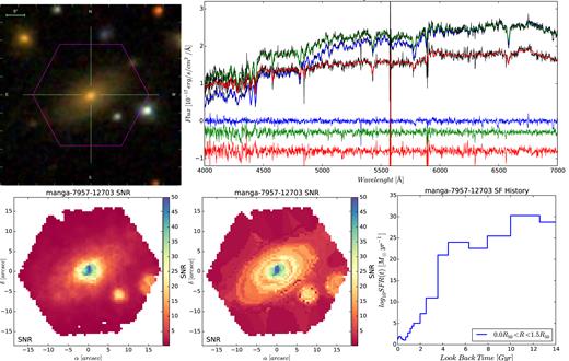
Similar figure as A1 for the galaxy manga-7957-12703.
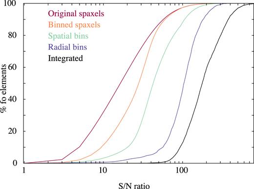
Cumulative functions of the signal-to-noise ratios for the original spaxels (red), the individual spaxels once performed the binning procedure (orange), the individual spatial bins or tessellas (light green), radial binning the spectra in annular of 0.5 effective radius, like the ones shown in Figs A1 and A2 (dark blue), and the integrated spectra across the entire FoV (black).
Due to the pseudo-stochastic nature of fit3d analysis (Sánchez et al. 2016a), the tessellas with lower S/N (∼10) present a lower precision in the derivation of the stellar population properties, and in particular the SFHs. This corresponds to just a few percentage (∼5 per cent) of the final tessellas, as appreciated in Fig. A3. Even more, the stacking of the derived models and their corresponding properties are a good representation of the data. This is illustrated in Figs A1 and A2, upper-right panel, where it is shown the average spectral within three different apertures together with the average of the individual models derived for the individual tessellas at the same apertures. We should remark here that we do not show a fitting to the average spectra, but an average of the results of the individual fits. The precision with which the average of the models describe the average spectra is remarkable. Indeed, the residuals of the subtraction of the data to the average of the models is better for the outer-rings than for the inner ones. This reflects that indeed the S/N of the average spectrum in the outer-ring is larger than that of the inner ones, and that using tessellas of lower S/N does not produce an appreciable bias in the average model. Therefore, we are confident of the stellar population model derived using this approach, in particular for the integrated properties.
Finally, as an illustration of the differences derived by the analysis for these two different galaxies considered, Figs A1 and A2 show their integrated the SFHs as they are originally derived by pipe3d without any of the corrections described in this article (i.e. in terms of sampled time ranges). It is clear that manga-7443-12704 has formed stars more recently than manga-7957-12703, what is it is reflected in the colours exhibited by the two galaxies in the SDSS images included in Figs A1 and A2.
APPENDIX B: EFFECTS OF SELECTING THE IONIZING SOURCE IN THE DERIVATION OF THE SFRH α
We perform a comparison between the derived SFRs using the dust-extinction corrected H α luminosity integrated along the optical extension of the galaxies and the values estimated by selecting only those regions where ionization is classified as star-formatting (H ii-like) on the kpc scales of the MaNGA data. As extensively discussed in Sánchez et al. (2017) and references therein, the selection of the source of ionization is not simple, even given all the line ratios accessible with the MaNGA data. In particular, for regions with low EW(H α) the best we can do is to indicate that it unclear if the gas is ionized by star formation. However, the contrary cannot be stated. Therefore, excluding those regions from the H α budget to derive the SFR could lead us to wrong results. In any case, we performed the current comparison to constrain the possible effects of this selection.
Fig. B1 shows the distribution of SFRs derived using the two different procedures. There is very good agreement between both quantities, following an almost one-to-one relation, with a dispersion of ∼0.2 dex and a global offset of ∼0.01 dex. This difference is even smaller for galaxies dominated by star formation ionization in their integrated properties (∼50 per cent of the galaxies), with no offset and a difference lower than a 2 per cent in the measurements. For those galaxies dominated by LINER-like ionization there is a larger difference, with an offset of ∼0.16 dex and a dispersion of 0.29 dex. However, for those galaxies we cannot guarantee that the ionization comes from SF or other sources of ionization, and in most cases they will be classified as retired, as we described in Section 4.1. Therefore, the selection of any of both methods to derive the SFRH α will not affect the results. Finally, for the ≤100 AGNs detected in MaNGA (Mallmann et al. 2018; Sánchez et al. 2018) we find a significant offset, of the order of ∼0.5 dex. However, as in the case of the RGs we cannot guarantee that part of this flux is due to SF, we can only determine that it is not the dominant source of the ionization. Including or removing them from the total number of analysed galaxies does not produce any significant different. For a comparison with single aperture cosmological surveys, where mixing of ionization does not guarantee that they would be classified as AGNs (e.g. Davies et al. 2016b), we prefer to keep them in the described analysis and stick to the integrated quantity described in Section 3.1.
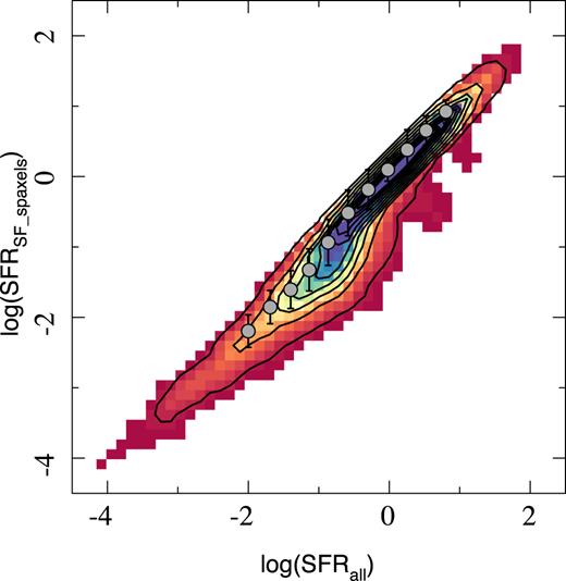
Density map showing the distribution of the SFRs based on the dust-corrected H α luminosity selecting only those spaxels fully compatible with being ionized by star formation (SFR|$_{\mathrm{ SF}\_\mathrm{ spaxels}}$|) versus just integrating through all the optical extent of the galaxies (SFRall). The contours illustrate the density of points, with the same contour encircling a 95 per cent of the points, with a decrease of 20 per cent in the fraction of points between each consecutive contour. The grey circles indicate the mean values in a bins of ∼0.3 dex in SFR, which the errorbars indicate the standard deviations around these mean values.
APPENDIX C: RELATION BETWEEN THE SFRH α AND SFRssp
In this article, we use SFRs derived at each cosmological time for galaxies based on the multi-SSP analysis outlined in Section 3 (i.e. SFRssp). For comparison purposes, when discussing the distribution of galaxies in the SFR–M* diagram at |$z$| ∼ 0, in Section 4.1, we make use of the SFR derived based on the dust-extinction corrected H α luminosities, presented in 3.1 (i.e. SFRH α). Both quantities do not present a one-to-one correspondence, as already indicated. We explore here the relation between both quantities and discuss the nature of their differences.
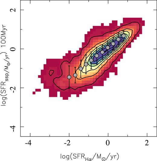
Density map showing the distribution of the SFRs derived using the SSP analysis (SFRssp) versus the SFRs estimated from dust-corrected H α luminosity (SFRH α). The contours illustrate the density of points, with the same contour encircling a 95 per cent of the points, with a decrease of 20 per cent in the fraction of points between each consecutive contour. The grey circles indicate the mean values in a bins of ∼0.3 dex in SFR; errorbars indicate the standard deviations around these mean values.
These differences are a consequence of: (i) The different stellar libraries adopted in the current study compared to the one used for the SFRH α calibrator, since this would change the correspondence between the optical emission (analysed in the current study) and the UV emission (considered in the SFRH α calibration). (ii) The amount of ionizing photons that depends on assumptions of the emission in the UV from young stars to derive that calibrator too. This depends strongly on the effects of the metallicity that has not been discussed here. Most of the calibrations of the SFR based on the H α luminosity are anchored to the solar metallicity (Kennicutt 1998). However, the UV luminosity output by a stellar population depends on its metallicity, which affects stellar temperatures and line blanketing. Generally speaking, less-metal-rich stars produce more UV light (e.g. Madau & Dickinson 2014). The amplitude of this effect is not insignificant, and depends on the details of the SFH, but in general, for the same SFR, less-metal-rich galaxies would present more ionizing photons and therefore larger H α luminosities, and the contrary for metal-rich galaxies. In contrast to the SFRH α estimate, our derivation of the SFRssp considered metallicity as part of the decomposition of the stellar population using the multi-SSP analysis. This would indeed generate a difference between both estimations of the SFR. (iii) The time-scale used to derive the SFR (as we have shown before), and the differences between the assumed SFHs adopted for the calibration of the relation between the H α luminosity and the SFR (Kennicutt 1998), and the reconstructed SFHs that could be derived from our stellar decomposition analysis. Although the conversion factor between SFR and H α luminosity is almost independent of the considered SFHs (e.g. section 2.3 of Kennicutt 1998), its correspondence with the SFRssp derived at different time-scales depends strongly on the shape of that SFHs. We should recall here that we have not assumed any particular shape for the SFH, although those could be reconstructed from the weights of the decomposition based on the multi-SSP analysis. Finally (iv) the differences between the assumed conditions of the ionized gas to derive the SFRH α calibration (Case B recombination, Te = 104 K Kennicutt 1998) and the real conditions of the observed ionized gas would produce significant differences. Just changing the geometry of the ionized gas distribution around the young stellar clusters would produce significant differences in the derived emission line fluxes (e.g. Morisset et al. 2016). All together it is not surprising that the two derivations of SFR exhibit differences. This is quite usual when comparing different calibrations (as clearly illustrated by Speagle et al. 2014; Catalán-Torrecilla et al. 2015; Davies et al. 2016a). Indeed, when comparing with cosmological simulations we found a similar discrepancy between both estimations of the SFR (Ibarra-Medel et al. in preparation). The derived relation has been included for future reference, but it is not used in the current study.
APPENDIX D: EVOLUTION OF THE SFMS SEGREGATED BETWEEN SFGs AND RGs
We explored the evolution of the SFMS with cosmic times in Section 4.2, for both the full sample of galaxies and the two subsamples of currently (z ∼ 0) SFGs and RGs. For clarity, we showed the distribution in the SFR–M* plane only for the full sample (Fig. 4). The same distribution for the two subsamples of SFGs and RGs are shown in Figs D1 and D2. The results of the analysis of the SFMS for those two subsamples of galaxies are listed in Table 1.
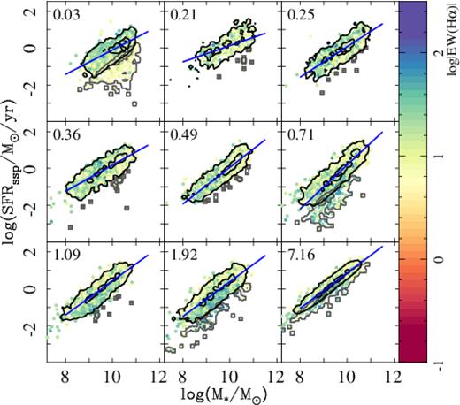
Distribution of the star formation rate (SFRssp) versus integrated stellar mass, as shown in Fig. 4 for the same redshift bins, here only for those galaxies that are star-forming at the observed time (|$z$| < 0.04). Symbols and labels are the same. As in the previous figure, for clarity, only those points with an error in the SFR lower than 0.2 dex have been included.
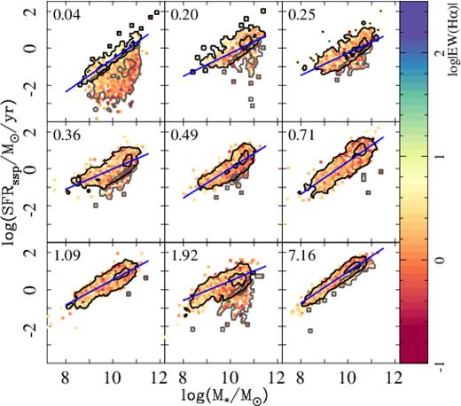
Distribution of the star formation rate (SFRssp) versus integrated stellar mass, as shown in Fig. 4 for the same redshift bins, here only for those galaxies that are retired at the observed time (|$z$| < 0.04). Symbols and labels are the same. As in the previous figure, for clarity, only those points with an error in the SFR lower than 0.2 dex have been included.
APPENDIX E: VOLUME CORRECTIONS
In Section 4.4, we derived the cosmic SFR density and the stellar-mass density as predicted from archaeological methods for ∼4000 local galaxies from the MaNGA survey. The MaNGA survey is a sample with approximately equal numbers of galaxies at a fixed stellar mass. In other words, MaNGA has approximately a flat stellar-mass distribution. In this appendix we, briefly, describe the volume corrections applied in order to project the mass distribution from MaNGA into a galaxy stellar-mass function, GSMF, that would be measured from a volume-limited sample that is complete in stellar mass. Here, we use the stellar masses, M*, galaxy colours, g − r and redshifts |$z$| from Blanton et al. (2017). We use K-corrected magnitudes at |$z$| = 0 tabulated in Blanton et al. (2017). In addition, we introduce the empirical model for the E-correction at |$z$| = 0 described in Dragomir et al. (2018). Finally, we derive the GSMF from the galaxy sample in Blanton et al. (2017) denoted hereafter as ϕ*(M*). We will use this model of the GSMF to estimate the expected number of galaxies as a function of redshift and stellar mass.
In a volume-limited sample that is complete in stellar mass, the GSMF can be simply estimated as ϕ*(M*)d log M* = Ng(M*)/V, where Ng is the observed number of galaxies with masses between log M* ± d log M*/2 and V is the co-moving volume of the observed sample. In the case of the MaNGA survey, the above is not true and using the above estimator would lead to an incorrect GSMF. Note, however, that is possible to use the above estimator to determine the average fraction of galaxies that are expected for a given M*, |$z$|, and g − r from the MaNGA sample to the expected number of galaxies that fully samples the GSMF, fm. While this fraction depends on the above three factors, in order to simplify our discussion, we consider next the case in which the fraction, fm depends only on |$z$| and M* leaving the general case to the end of this section.
In the general case in which fm also depends on galaxy colours, the above procedure is still valid. The fraction will be given by fm(M*, |$z$||c) = 〈ϕM, *(M*|c)〉/ϕ*(M*|c) where c indicates that we are estimating our GSMF as a function of colour. For our final volume correction we have divided the sample into five colour bins between 0 < g − r < 1.2.
APPENDIX F: COSMIC SFR HISTORY USING ORIGINAL REDSHIFT BINS
The cosmic SFR history discussed in Section 4.4 was built using a different set of redshift bins as the ones used to analyse the evolution of galaxies along the SFR–M* diagram, shown from Section 4.2 to Section 4.3. These new redshift bins were introduced to maximize the coverage along cosmological times of the sampled parameter, ΨSFR, t. However, the analysis could be performed using exactly the same redshift bins used before, to the penalty of a poorer time sampling. Fig. F1 shows the result of this analysis. As expected the number of bins is reduced by a factor 2, and the trends shows in Fig. 9 are less clearly defined. However, the main results discussed in Section 4.4 hold. The global rise of ΨSFR, t along earlier cosmological times, with a broad peak around |$z$| ∼ 1–3, and the differences outlined between the cosmic evolution of RGs0 and SFGs0 remain visible when using the original redshift bins.

APPENDIX G: COSMIC SFR HISTORY WITHOUT GALAXY SELECTION
As indicated in Section 4.4, to build the cosmic SFR history from our analysis we selected only the SFGs at each look-back time for reasons already indicated in that section. To evaluate the impact of that selection in the derived ΨSFR, t we repeated the analysis without performing any galaxy selection, thus, assuming that (1) all the measurements of SFR at any time are reliable and (2) that our survey is deep enough to measure the SFR of all those galaxies. Then, we added quadratically the difference between the values derived using this estimate with the ones derived by selecting only the SFGs to our error budget. We claimed that the main difference is present in the two higher redshift bins. Fig. G1 illustrates that claim by showing the ΨSFR,t derived by adopting no sample selection. As already indicated in Section 4.4, the main trends described for this distribution for |$z$| < 3 hold, without any significant modification. There are some fluctuations of the values, most of them consistent with the original distribution for both the full sample and the SFGs0 and RGs0 subsamples. As already indicated the main difference is in the two higher redshift bins, in which instead of the decrease described before we see either a rising or a flat distribution. We should note that this is consistent with the SFHs shown in Fig. 2, within the errors. Based on this analysis we claim along the article that out SFHs are not reliable beyond |$z$| > 3.
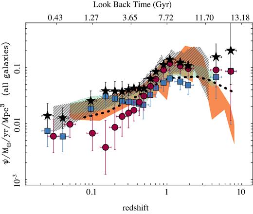
Similar figure to Fig. 9, showing the cosmic evolution of the SFR density and using the same symbols. Here, no cut is made in the sSFRt of the targets. Note that most of the differences between these two figures are found at very high redshifts.
APPENDIX H: COSMIC SFR HISTORY WITHOUT GALAXY REPETITION
We estimated the cosmic SFR history of the universe in this article by treating our collection of SFRs and stellar masses as an observed cosmological survey. Thus, when we select synthetic galaxies in a given redshift bin, the values could be due to the same original galaxy that is sampled several times in that given redshift bin. This introduces a correction factor for the number or repetitions of a galaxy within each redshift bin (Section 4.4). Fig. H1 shows the distribution of this correction factor, defined in equation (3) along the redshift. To avoid the introduction of this correction factor a different approach would be to average the SFRs coming from the same galaxy within each bin to produce the same mathematical result. However, this would not respect the basis of our approach, i.e. to treat the data set in a similar way as cosmological surveys are treated.
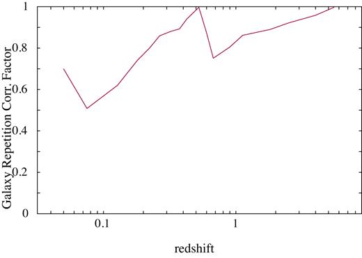
Galaxy repetition correction factor introduced in equation (2) to derive the cosmic star formation rate density to take into account the repetition of the same galaxies sampled at different look-back times in the same redshift bin.
A different approach would be to allow each galaxy to be sampled only once in each redshift bin. This will introduce a certain degree of uncertainty, since it would require selecting one of the sampled SFRs. This approach is less precise, and can lead to considerable biases depending on how this selection is done. However, it can be tested to illustrate if the current procedure provides better results, and if so, at what redshifts (i.e. matching better to the values reported from cosmological surveys). For this test we repeated our estimates of ΨSFR, t following the prescriptions shown in Section 4.4 with the only difference that when a galaxy is sampled once it is not allowed to be sampled again. Thus, we forbid repetition of the same original galaxy in a given redshift bin. Since by construction the data set is ordered by redshift, those values correspond to smaller look-back times within each bin. Since in general most of the SFHs of galaxies exhibit a decline in SFR with the redshift, the accepted values correspond with lower SFRs than in the original calculation. Fig. H2 shows the result of the calculation. In general, the more affected bins are between |$z$| < 0.1 and |$z$| > 1.5, as expected since those bins are the ones for which the galaxies are repeated most frequently. In particular, this approach (biased, as indicated before), underpredicts the cosmic SFR in those bins where repetitions are frequent, highlighting the fact that we have selected preferentially lower values of SFR than is representative for a given galaxy within a given redshift bin.
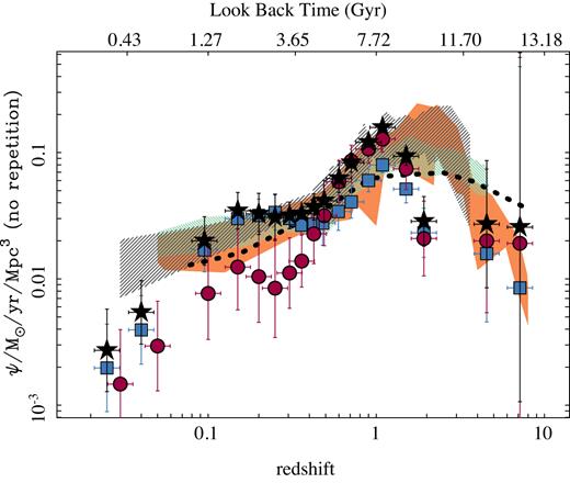
Similar figure as Fig. 9, showing the cosmic evolution of the SFR density, using the same symbols, but this time without allowing repetitions of values extracted from the analysis of the stellar populations of the same original galaxy. In this particular approach, we adopted the first (lower redshift) value encounter for a particular galaxy as the one that it is representative of the different SFRs sampled within the considered redshift bin.
In summary, the considered correction factor is required due to the adopted approach in which we treat our data set as a synthetic cosmological survey, and therefore each synthetic galaxy should be weighted individually, irrespectively of the number of times that it is sampled within a particular redshift range.
Despite of the clear bias introduced by the approach adopted in this new derivation of ΨSFR, t, and the fact that the numerical values depart more from the ones reported by cosmological surveys, it is interesting to note that most of the qualitative properties of the cosmic SFR history reported along this article are still the same: (1) The reported distribution seems to follow at least qualitatively the known shape for the Madau curve. (2) The peak in the cosmic SFR density seems to be at a slightly lower redshift than the one reported in the literature. (3) RGs and SFGs in the Local Universe present different contributions to ΨSFR, t, with the former being more active in the past, and having a sharper evolution.
