


Abstract
We present the complete sample of stripped-envelope supernova (SN) spectra observed by the Lick Observatory Supernova Search (LOSS) collaboration over the last three decades: 888 spectra of 302 SNe, 652 published here for the first time, with 384 spectra (of 92 SNe) having photometrically determined phases. After correcting for redshift and Milky Way dust reddening and reevaluating the spectroscopic classifications for each SN, we construct mean spectra of the three major spectral subtypes (Types IIb, Ib, and Ic) binned by phase. We compare measures of line strengths and widths made from this sample to the results of previous efforts, confirming that O i λ7774 absorption is stronger and found at higher velocity in Type Ic SNe than in Types Ib or IIb SNe in the first ∼30 days after peak brightness, though the widths of nebular emission lines are consistent across subtypes. We also highlight newly available observations for a few rare subpopulations of interest.
1 INTRODUCTION
Hydrogen-poor supernovae (SNe) showing strong Si ii λ6355 absorption and presumably arising from cataclysmic thermonuclear white dwarf explosions (Type Ia SNe) have long been of intense interest to observers for their cosmological utility (e.g. Riess et al. 1998; Perlmutter et al. 1999), while a few dozen relatively nearby hydrogen-rich SNe arising from the deaths of massive stars (Type II SNe) have provided observers a powerful perspective on to the physics of these systems (e.g. McCray 1993, 1997; Smartt et al. 2009; McCray & Fransson 2016). In contrast, hydrogen-poor SNe arising from massive stellar deaths (the stripped-envelope SNe: Type IIb, with H easily visible at early times and He lines later; Type Ib, with no H but showing obvious He lines; and Type Ic, with neither obvious H nor obvious He – for more thorough discussions of SN spectral types see Filippenko 1997; Gal-Yam 2017) have historically proven less amenable to detailed observational studies than their hydrogen-rich counterparts, and have been less intensely studied than the cosmologically useful SNe Ia.
These stripped-envelope SNe provide a powerful window into the physics that govern the rapidly evolving and often chaotic end-stages of massive stellar evolution, but many puzzles remain about their progenitors and host-galaxy environments. Sana et al. (2012) show that ∼33 per cent of massive O-type stars in the Milky Way undergo significant envelope stripping via Roche lobe overflow, in good agreement with the fraction of core-collapse SNe classified as stripped-envelope in a volume-limited sample (Smith et al. 2011; Shivvers et al. 2017a); it appears that the most common progenitors of normal SNe IIb, Ib, and Ic arise within binary systems (e.g. Yoon, Woosley & Langer 2010). However, stripped-envelope SNe are heterogenous; it is likely that several progenitor channels contribute to the observed SN populations. For example, a small fraction of the SNe Ib likely arise from isolated and very massive progenitors that have lost their envelopes through a vigorous line-driven wind (e.g. PTF10qrl and iPTF15cna; Conti 1975; Fremling et al. 2018), while at least some members of the SN Ibn subclass arise from systems where explosive outbursts have contributed to their envelope stripping (e.g. SN 2006jc; Foley et al. 2007).
Even when restricting the discussion to the relatively common classes (Types IIb, Ib, and Ic), many questions remain. The key observational indicators used to discriminate between subtypes exhibit confounding traits: the strength of the Hα feature in SN spectra is a sensitive and easily saturated indicator of the presence (or lack) of hydrogen, making it difficult to discern whether SNe Ib and IIb are truly separate populations or instead lie along a continuum with the hydrogen-rich Type II SNe, while the optical features of He i may not be present though the ejecta are helium-rich (e.g. Dessart et al. 2012a). These effects sometimes make the physical interpretation of observational trends between subtypes difficult, but careful studies of the spectra of these diverse and multifarious populations help us to tease apart their complexities.
Many single-object papers examining stripped-envelope SNe have been written, but for years the work of Matheson et al. (2001), analysing 84 spectra of 27 SNe, provided researchers the only large multi-object sample of optical spectra. The more recent work of Modjaz et al. (2014), however, has greatly expanded the set of publicly available data by publishing 645 spectra of 73 SNe, and the very recent work of Fremling et al. (2018) has contributed a valuable analysis of 507 spectra of 173 events, all having a measured date of peak brightness. Interest in the study of the bulk properties of these relatively poorly understood events has been reignited by these samples (e.g. Liu et al. 2016; Modjaz et al. 2016; Stritzinger et al. 2018a,b; Taddia et al. 2018).
This paper builds on past efforts to understand stripped-envelope SNe by presenting the largest single data set yet released (including numerous spectra obtained at late times) and analysing this data set to interpret the underlying physical mechanisms driving the subtype divisions among stripped-envelope SNe. The observational study of all SNe via their spectra has long been the focus of our SN research group at U.C. Berkeley. Over the last three decades we have deployed the resources of the Lick and Keck Observatories toward this goal, and with this paper we present essentially all stripped-envelope SN spectra observed by the University of California (U.C.) Berkeley / Lick Observatory Supernova Search (LOSS; Filippenko et al. 2001) effort, from 1985 up through the end of 2015, including 888 spectra of 302 SNe. A fraction of these data (236 spectra) has already been examined, either by Matheson et al. (2001, who published the pre-2000 Berkeley data) or as part of single-object studies, but we include them here again to provide a coherent data set observed with similar observational techniques and reduced via similar procedures. A date of peak brightness can be measured for 92 of the SNe having spectra published here, either from our own internal photometric database or previously published data, allowing us to label 384 spectra with their phases. These spectra are made publicly available through the Berkeley Supernova Database1 (the SNDB, first described by Silverman et al. 2012a), the Weizmann Interactive Supernova data REPository2 (WiseREP, Yaron & Gal-Yam 2012), and the Open Supernova Catalogue3 (Guillochon et al. 2017). Here we follow similar efforts from the past few years which have examined and made publicly available the accumulated Berkeley samples of Type Ia SNe (Silverman et al. 2012a,c; Silverman, Kong & Filippenko 2012b; Silverman & Filippenko 2012; Silverman, Ganeshalingam & Filippenko 2013) and Type II SNe (Faran et al. 2014a,b).
This paper is laid out as follows. Section 2 describes our observational methods and data-reduction procedures, including our efforts to determine robust spectral types and phases. We describe and present the data set itself in Section 3. In Section 4, we compare analyses of this sample to previously published works; we present continuum-normalized mean spectra of SNe IIb, Ib, and Ic in four different phase bins, and we discuss a few rare subpopulations of interest that are represented in this data set.
2 OBSERVATIONS, DATA REDUCTIONS, AND CALIBRATIONS
Our data include observations obtained with a variety of instruments mounted on the telescopes at Lick and Keck Observatories: the UV Schmidt spectrograph (1987–1992; Miller & Stone 1987) and the Kast Double Spectrograph (since 1992; Miller & Stone 1993) on the Shane 3 m telescope, and the Low Resolution Imaging Spectrometer (LRIS; Oke et al. 1995), the Echellette Spectrograph and Imager (ESI; Sheinis et al. 2002), and the DEep Imaging Multi-Object Spectrograph (DEIMOS; Faber et al. 2003), on the two Keck 10 m telescopes.
Taking advantage of a few nights on the Shane 3 m every lunar cycle, augmented by occasional nights with one of the Keck telescopes, our group strives to maintain a steady cadence of observations for all of the SNe we study – Silverman et al. (2012a) describe our observing strategies in more detail. For the sample of spectra presented here, we calculate a typical (median) time lag of 14.8 d between successive observations of any given SN.
With a few exceptions, our spectra are flat-field corrected with dome flats and wavelength calibrated with observations of emission-line calibration lamps obtained each night (usually at the position of the science target), flux-calibrated via spectra of standard stars taken at an airmass comparable to that of the science target, and observed at the parallactic angle (Filippenko 1982) to minimize the effects of atmospheric dispersion.
The data-reduction procedures we use to transform the two-dimensional spectrogram measured by a CCD into a wavelength-calibrated, flux-calibrated, one-dimensional spectrum are similar across instruments and have changed only slowly over time – Silverman et al. (2012a) discuss these procedures in detail. The codes used to perform these reductions consist of a mixture of IRAF,4idl, and Python and are publicly available.5
2.1 Dates of peak brightness via photometry
Though precise determinations of the explosion dates are only rarely obtained for SNe, the date of peak brightness can often be observationally constrained. Here we attempt to date all of our spectra relative to the SN’s epoch of photometric peak so as to compare SN evolution across different events. For the SNe in our sample, we accumulate the light curves and observed dates of photometric peak we can find in the published literature or in our own (both published and unpublished) repository of photometry.6
Several studies have documented a wavelength dependency of the measured time of peak brightness (e.g. Drout et al. 2011; Bianco et al. 2014), with bluer passbands peaking before the red, and our accumulated data support those trends. Our data come from diverse sources, with the dates of peak constrained in different passbands for different events, and so we fit for this wavelength dependence and strive to place all of these different measures on a similar scale.
First, we collect the published dates of peak brightness from all available literature sources. If error bars on the value were not published (as was often the case) we attempted to obtain the light-curve data and fit for the peak ourselves. Secondly, we collected all as-yet unpublished photometric data that constrain the date of peak for these SNe from our SNDB repository. To fit for a peak, we require a light curve with at least two data points showing the rise and turnover. (The declines of these light curves are generally well-sampled, but the early rise and the peak itself are often missed.) We model the light curve with a quadratic polynomial and we restrict our fit to observations taken within ±10 d of peak brightness.
We then chose a specific wavelength at which to normalize the diverse light-curve passbands; examining our data set; we find that normalizing all data to the date of peak brightness as measured at 6000 Å produces a reasonable compromise by minimizing the number of SNe for which we must significantly extrapolate in wavelength (6000 Å is close to the central wavelengths of both the KAIT clear and R passbands; Li et al. 2003). To do this, we take all SNe with estimates of peak measured in four or more passbands with central wavelengths both above and below 6000 Å, and we then fit for the wavelength dependence of the peak-brightness date for each SN. We utilize Gaussian-process regression to propagate our uncertainties through the interpolation and produce measures and uncertainty estimates for the date at which the SN light curve peaked in the virtual passband centred at 6000 Å, t6000.
For each individual light curve, we calculate the time delay between t6000 and the date of peak brightness through the given passband (Δt). For each passband, we then take the weighted average of the Δt found across different SNe to infer that passband’s phase of peak relative to t6000, and we report the standard deviation as an estimate of our uncertainties. See Table 1 and Fig. 1 for our results and the number of SNe used to reach them.
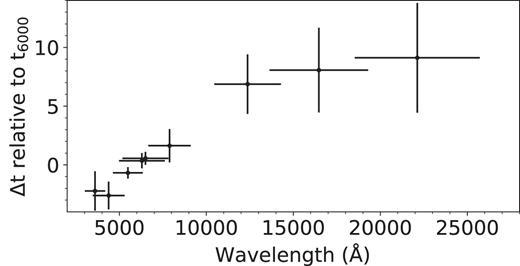
Offsets between peak brightness as measured in each passband and the peak at 6000 Å (t6000). Error bars in Δt represent the standard deviation across measures from all SNe, and we illustrate the effective widths of each passband using error bars in wavelength.
Phase of peak by passband.
| Passband | Δt ±1σ† | No. of SNe |
|---|---|---|
| (d) | ||
| U | −2.2 ± 1.7 | 6 |
| B | −2.6 ± 1.2 | 17 |
| V | −0.7 ± 0.5 | 20 |
| clear | 0.3 ± 0.7 | 20 |
| R | 0.6 ± 0.6 | 20 |
| I | 1.6 ± 1.4 | 20 |
| J | 6.9 ± 2.5 | 7 |
| H | 8.1 ± 3.6 | 7 |
| K | 9.1 ± 4.7 | 6 |
| Passband | Δt ±1σ† | No. of SNe |
|---|---|---|
| (d) | ||
| U | −2.2 ± 1.7 | 6 |
| B | −2.6 ± 1.2 | 17 |
| V | −0.7 ± 0.5 | 20 |
| clear | 0.3 ± 0.7 | 20 |
| R | 0.6 ± 0.6 | 20 |
| I | 1.6 ± 1.4 | 20 |
| J | 6.9 ± 2.5 | 7 |
| H | 8.1 ± 3.6 | 7 |
| K | 9.1 ± 4.7 | 6 |
†Relative to t6000.
2.2 Spectroscopic classifications
The exact subtype definitions best used to discriminate between stripped-envelope SNe and highlight their underlying physics have long been debated and discussed in the literature (e.g. Filippenko, Porter & Sargent 1990; Wheeler & Harkness 1990; Wheeler et al. 1994; Clocchiatti et al. 1996; Matheson et al. 2001; Branch et al. 2006), and updates to previously announced spectral types are often justified when performing comparisons between types (e.g. Modjaz et al. 2014; Shivvers et al. 2017a). We therefore strive to confirm and, if required, update the spectral type for all of the SNe in our sample.
We rely heavily upon the SuperNova IDentification code (snid; Blondin & Tonry 2007) and follow the classification guidelines laid out by Shivvers et al. (2017a). We use the bsnip v7.0 snid templates (Silverman et al. 2012a) augmented by the Liu & Modjaz (2014) stripped-envelope templates (and following all suggestions from their table 4). Given the difficulty of classifying historical SNe having limited observational coverage, we assign a single type only when possible (using all data available on each SN, both ours and previously published observations); if multiple types are reasonable we list them all and do not choose between them.
We follow a multi-step process for each of the spectra in our sample, iteratively attempting to obtain spectral type and subtype classifications and (if possible) age estimates. For each SN represented in our sample, we then examine the set of results found for all of the spectra of the object and choose the best classification. In detail, we undertake a multistep process for each spectrum similar to that described by Silverman et al. (2012a). We first run snid, setting the redshift to that of SN’s host galaxy (using the forcez keyword) and demanding a minimum rlap value of 10. If this produces a single preferred type (if the type of the best-match template matches the most common type amongst all spectra which pass our rlap threshold, and if >50 per cent of the templates passing that threshold are of the same type), we record the preferred type. If there are not at least three matches with rlap >10, we relax the threshold to rlap >5 and repeat. If the above process does not produce a single preferred classification we record the set of reasonable types and move on.
However, if a single type is successfully determined, we then attempt to determine a subtype. We again run SNID (demanding rlap >10) and consider only correlations with templates of the type as determined above (taking advantage of the usetype keyword) and again relaxing the rlap threshold to 5, if needed. If a single subtype is preferred (under the same requirements as above), we adopt it; if not, we do not record a subtype classification for this spectrum.
We then accumulate all of the spectrum-specific classification results for each SN and determine whether a single classification is preferred for each object. For those SNe with conflicting type classifications amongst their various spectra, we prefer the classifications obtained at phases between peak brightness and +50 d post-peak (as indicated by either light-curve peak measures or the ages of the best-match SNID templates; see below), since those are the phases that are observationally best constrained and which have the best coverage in the SNID template set.
If spectra exist only at phases where distinctions are difficult to draw, we record multiple possible types. If multiple conflicting classifications (or no trustworthy classifications) exist for a single object, we examine all available data in more detail, and if a convincing classification can be obtained by incorporating light-curve information, we do so (in the same manner as Shivvers et al. 2017a). Note that few SNID templates exist for many of the rarer subtypes (see Section 4.6). In most cases, the spectra for these subtypes resulted in conflicting classifications each having low rlap values, and the examples discussed in Section 4.6 were predominantly discovered and classified by hand after our automatic classification methods failed. If multiple types remain plausible, we list them all; the resulting type assignments are given in Table 2, and for several SNe they differ from those first announced in the International Astronomical Union Circulars (IAUCs; also CBETs) and Astronomer’s Telegrams (ATels).
The SNe in our sample.
| Name | Type | Host | Redshift | E(B-V)MW | Date of Peak | No. of spectra |
|---|---|---|---|---|---|---|
| (MJD ±1σ) | ||||||
| SN 1985F | Ib | NGC 4618 | 0.00180a | 0.018 | – | 1 |
| SN 1987K | IIb | NGC 4651 | 0.00266b | 0.023 | 47009.6 ± 7.2c | 7 |
| SN 1987M | Ic | NGC 2715 | 0.00441d | 0.022 | – | 5 |
| SN 1988L | Ic | NGC 5480 | 0.00638e | 0.016 | – | 3 |
| SN 1990aa | Ic | MCG+05-03-16 | 0.01647d | 0.046 | – | 3 |
| SN 1990aj | Ib/Ic | NGC 1640 | 0.00536f | 0.030 | – | 1 |
| SN 1990B | Ic | NGC 4568 | 0.00750g | 0.028 | – | 4 |
| SN 1990U | Ib | NGC 7479 | 0.00794h | 0.097 | 48094.2 ± 7.2c | 13 |
| SN 1991A | Ic | IC 2973 | 0.01059d | 0.017 | 48246.0 ± 7.2c | 6 |
| SN 1991ar | Ib | IC 49 | 0.01521h | 0.019 | 48490.6 ± 7.2c | 2 |
| SN 1991D | Ib | LEDA 84044 | 0.04175b | 0.053 | – | 2 |
| SN 1991L | Ic | MCG+07-34-134 | 0.03054e | 0.012 | – | 1 |
| SN 1991N | Ic | NGC 3310 | 0.00300i | 0.019 | – | 4 |
| SN 1993J | IIb | NGC 3031 | −0.00047j | 0.069 | 49095.5 ± 0.6k | 50 |
| SN 1994ai | Ib/Ic | NGC 908 | 0.00500f | 0.022 | – | 1 |
| SN 1994I | Ic | NGC 5194 | 0.00150g | 0.031 | 49451.3 ± 0.1l | 15 |
| SN 1995bb | Ib/Ic | Anon J001618+1224 | 0.00580m | 0.096 | – | 1 |
| SN 1995F | Ib | NGC 2726 | 0.00487b | 0.031 | 49772.8 ± 7.2c | 4 |
| SN 1996cb | IIb | NGC 3510 | 0.00240g | 0.026 | 50452.7 ± 1.0n | 4 |
| SN 1997B | Ic | IC 438 | 0.01041h | 0.062 | – | 1 |
| SN 1997dc | Ib | NGC 7678 | 0.01167d | 0.042 | – | 1 |
| SN 1997dd | IIb | NGC 6060 | 0.01466e | 0.070 | – | 1 |
| SN 1997dq | Ic | NGC 3810 | 0.00300o | 0.038 | – | 4 |
| SN 1997ef | Ic-BL | UGC 4107 | 0.01169h | 0.036 | – | 6 |
| SN 1997ei | Ic | NGC 3963 | 0.01060p | 0.019 | – | 2 |
| SN 1997X | Ib | NGC 4691 | 0.00375q | 0.024 | 50483.8 ± 7.2c | 1 |
Notes. (Truncated; full table available online)
References: [a]: Lennarz, Altmann & Wiebusch (2012), [b]: Paturel et al. (2002), [c]: SNID, [d]: Falco et al. (1999), [e]: Adelman-McCarthy et al. (2011), [f]: Meyer et al. (2004), [g]: Poznanski et al. (2002), [h]: Modjaz et al. (2011), [i]: Beckmann et al. (2003), [j]: Matheson et al. (2000c), [k]: Richmond et al. (1994), [l]: Richmond et al. (1996), [m]: Hakobyan et al. (2012), [n]: Qiu et al. (1999), [o]: Bosnjak et al. (2006), [p]: Springob et al. (2005), [q]: Adelman-McCarthy et al. (2008).
2.3 Dates of peak brightness via SNID
For those SNe without a photometrically measured date of peak brightness, but with a single clearcut type and subtype classification, we use SNID (and its library of template spectra having photometrically determined dates of peak brightness) to estimate the age of the SN at each epoch of spectroscopy. We rerun snid, comparing only against templates of the correct type and subtype, and demanding rlap≥0.75 × rlapbest, where rlapbest is the rlap value of the best-match template. For each SN, we accumulate the implied dates of peak brightness based upon the ages estimated for the spectra. If there are three or more such estimates, we take their median as our best estimate.
We assess the quality of our SNID-determined peak-brightness dates with the subset of SNe having both SNID-determined and photometrically measured peak dates. Amongst the 30 events with both of the above, the mean discrepancy was 0.8 d (SNID has a slight bias toward predicting a date of peak brightness earlier than that measured from the light curve), and the distribution of differences exhibited a standard deviation of 7.2 d (see Fig. 2). For the 31 SNe without a photometrically measured date of peak brightness and with a SNID-determined one, we adopt the SNID value with estimated error bars of 7.2 d (in most of these cases, the SN was first discovered post-peak).
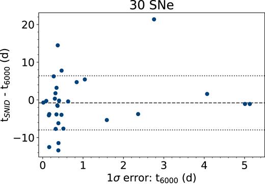
The difference between dates of peak brightness as predicted by SNID (tSNID) and as inferred at 6000 Å (t6000), plotted against the 1σ error bars on the measured date of peak brightness.
2.4 Redshift and dust reddening corrections
We apply redshift corrections to all of our spectra and analyse them in their host galaxy’s rest frame. For all but a few SNe in our sample, we are able to associate the event with its host galaxy and adopt the host’s previously published redshift measures, and for most of the remaining events we are able to measure the redshift directly from narrow galaxy emission lines within our spectra. However, both of these methods fail for SNe 2008gk and 2009ka; for these two events we infer the redshift via spectral cross-correlation using SNID.
We take the line-of-sight extinction arising within our Galaxy from the dust maps of Schlafly & Finkbeiner (2011), and we assume RV = 3.1 to correct each spectrum for Milky Way dust reddening (Cardelli, Clayton & Mathis 1989; O’Donnell 1994). The magnitude and wavelength dependance of dust reddening arising from within each SN’s host galaxy are largely unknown, however. A small number of spectra show narrow Na i D absorption lines from the host, but most do not, and doubt exists about the predictive power of this feature in low-resolution spectra like these (Poznanski et al. 2011; Phillips et al. 2013). We therefore do not attempt to correct for reddening within the host galaxy, and instead endeavour to perform analyses that do not depend upon exact flux determinations.
3 THE SAMPLE
Table 2 presents the sample of SNe included in this data release, our adopted classifications and dates of peak brightness (if available), and the values we used to perform redshift and dust-reddening corrections. Table 3 provides a description of the spectra included in our sample. Our research group utilizes a database of observations and associated metadata (the SNDB; Silverman et al. 2012a) to orchestrate our observational campaigns, to facilitate access to and analysis of our large repository of data, and to share those data publicly – all of the spectra described herein are publicly available through the SNDB web page (see footnote 1).
The spectra presented in this paper.
| Name | SN Type | Date | Phaseα | Instrument | Wavelength Range | Resolutionβ | Referenceγ |
|---|---|---|---|---|---|---|---|
| (ut) | (d) | (Å) | (Å) | ||||
| SN 1985Fδ | Ib | 1985-04-01 | – | Double spectrograph/ITS | 3180−10100 | 12 | Filippenko & Sargent (1986) |
| SN 1987K | IIb | 1987-07-31 | −1.8 ± 7.2 | UV Schmidt | 4280−7140 | 12 | Filippenko (1988) |
| SN 1987K | IIb | 1987-08-01 | −0.8 ± 7.2 | UV Schmidt | 4280−7140 | 12 | Filippenko (1988) |
| SN 1987K | IIb | 1987-08-07 | 5.2 ± 7.2 | UV Schmidt | 3200−8880 | 12 | Filippenko (1988) |
| SN 1987K | IIb | 1987-08-09 | 7.2 ± 7.2 | UV Schmidt | 4510−7570 | 12 | Filippenko (1988) |
| SN 1987K | IIb | 1987-08-12 | 10.2 ± 7.2 | UV Schmidt | 5960−7570 | 12 | Filippenko (1988) |
| SN 1987K | IIb | 1987-12-25 | 145.2 ± 7.2 | UV Schmidt | 6120−9270 | 12 | Filippenko (1988) |
| SN 1987K | IIb | 1988-02-24 | 206.2 ± 7.2 | UV Schmidt | 6040−9230 | 12 | Filippenko (1988) |
| SN 1987M | Ic | 1987-09-28 | – | UV Schmidt | 3130−10000 | 12 | Filippenko, Porter & Sargent (1990) |
| SN 1987M | Ic | 1987-11-22 | – | UV Schmidt | 3280−9100 | 12 | Filippenko et al. (1990) |
| SN 1987M | Ic | 1987-12-26 | – | UV Schmidt | 3180−9070 | 12 | Filippenko et al. (1990) |
| SN 1987M | Ic | 1988-02-25 | – | UV Schmidt | 3310−9220 | 12 | Filippenko et al. (1990) |
| SN 1988L | Ic | 1988-06-28 | – | UV Schmidt | 3500−9300 | 12 | Matheson et al. (2001) |
| SN 1988L | Ic | 1988-07-17 | – | UV Schmidt | 5970−9150 | 12 | Matheson et al. (2001) |
| SN 1988L | Ic | 1988-09-15 | – | UV Schmidt | 6000−9100 | 12 | Matheson et al. (2001) |
| SN 1990aa | Ic | 1990-09-27 | – | UV Schmidt | 3900−9850 | 12 | Matheson et al. (2001) |
| SN 1990aa | Ic | 1990-10-20 | – | UV Schmidt | 3900−7020 | 12 | Matheson et al. (2001) |
| SN 1990aa | Ic | 1991-01-23 | – | UV Schmidt | 3900−9800 | 12 | Matheson et al. (2001) |
| SN 1990aj | Ib/Ic | 1991-03-10 | – | UV Schmidt | 5800−8950 | 12 | Matheson et al. (2001) |
| SN 1990B | Ic | 1990-03-25 | – | UV Schmidt | 3950−9800 | 12 | Matheson et al. (2001) |
| SN 1990B | Ic | 1990-04-01 | – | UV Schmidt | 3950−9800 | 12 | Matheson et al. (2001) |
| SN 1990B | Ic | 1990-06-15 | – | UV Schmidt | 6720−9850 | 12 | Matheson et al. (2001) |
| SN 1990B | Ic | 1990-04-30 | – | UV Schmidt | 3930−9800 | 12 | Matheson et al. (2001) |
| SN 1990U | Ib | 1990-07-30 | 8.7 ± 7.2 | UV Schmidt | 3120−7500 | 12 | Matheson et al. (2001) |
| SN 1990U | Ib | 1990-07-31 | 9.7 ± 7.2 | UV Schmidt | 3120−9850 | 12 | Matheson et al. (2001) |
| SN 1990U | Ib | 1990-08-29 | 38.7 ± 7.2 | UV Schmidt | 3900−9850 | 12 | Matheson et al. (2001) |
Notes. (Truncated; full table available online)
αDays relative to peak brightness, if date of peak is constrained.
βEstimated average resolution across the spectrum.
γOriginal publications for already-published spectra.
δThis historical spectrum was observed under unique conditions – we exclude from our analyses below but we include it here for completeness.
The majority of SNe in this sample have only a few spectral observations each, though several well-observed examples of each subtype are also included – Fig. 3 shows the distribution of observation count across SNe in our sample. Our sample includes spectra taken within days of core collapse out to several years [for those SNe that show ongoing, luminous interaction with circumstellar material (CSM)]. Fig. 4 illustrates the phase coverage for spectra of those SNe having either a photometrically or SNID-measured peak-brightness date.
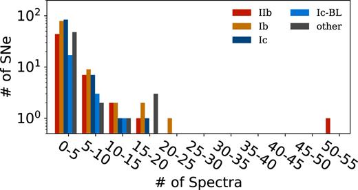
The distribution of spectral observation counts for SNe in our sample. Totals are binned over five-spectra intervals, and we group spectra of peculiar subtypes and of stripped-envelope SNe without a clearcut subtype classification together into the ‘other’ category.

The phase distribution of spectra having a measured date of peak brightness, grouped by spectral type and binned over 50-d intervals. Spectra having photometric peak dates are shown in solid, while the lighter shade also includes those with snid-determined peak dates. This plot is truncated at 450 days; a small number of observations exist at later phases.
4 RESULTS
Below we examine the evolution, relative to date of peak brightness, of several different observational signatures in order to probe the kinematics and composition of the ejecta and to compare to previous results. In summary, we confirm that the O i λ7774 feature has both a higher pseudo-equivalent width (pEW) and a higher characteristic velocity in SNe Ic than in SNe Ib or IIb, supporting the interpretation that SNe Ic are stripped further down toward the C-O core than SNe Ib/IIb but they explode with similar energies. However, we do not find supporting evidence for that scenario from an analysis of the nebular spectra: one may expect that SNe Ic, having lost more of their envelope but exploding at similar energies, would exhibit wider full width at half-maximum intensity (FWHM) measures at very late times than do the SNe Ib/IIb, which we do not see. We also highlight a few unique characteristics of this data set, including the large number of late-time spectra and the many spectra of rare SN subtypes released here.
4.1 Oxygen absorption
O i λ7774 absorption is readily apparent in the spectra of all three major stripped-envelope classes, and it provides several important insights into the underlying progenitor differences that give rise to these observational classes of SNe. We measure two characteristics of this oxygen absorption feature in our spectra: to compare line strength across SNe we calculate their pEW, and to compare ejecta velocities we calculate the relativistic Doppler velocity indicated by the wavelength of each absorption feature’s minimum (λmin). To obtain these measures, we follow the procedures outlined by Silverman et al. (2012b) using a set of supervized algorithms, and we visually inspect each measure to identify and correct errors.
Matheson et al. (2001) find the O i λ7774 absorption feature to be stronger in SNe Ic than SNe Ib and suggest a trend: that the strength of O i λ7774 absorption is inversely correlated with the degree of stripping experienced by the progenitor before core collapse. This finding was corroborated by Liu et al. (2016) and Fremling et al. (2018), and is confirmed again when analysing the data set presented here.
Fig. 5 shows the pEW measures for the SNe IIb, Ib, and Ic spectra in this data set having both a known phase and a clearly identifiable O i λ7774 feature, along with a rolling window mean and the associated standard deviations. (Note that for this and all following plots showing rolling window statistics, we ensure that no more than one measure per SN is shown in each bin, so as to focus on the variance between events.) At these phases, SNe Ic exhibit significantly stronger oxygen absorption than SNe Ib and IIb, and there appears to be a small but systematic difference between the line strengths in SNe Ib and SNe IIb, in good agreement with the scenario put forth by Matheson et al. (2001).
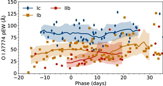
O i λ7774 pEW as a function of phase for SNe IIb, Ib, and Ic. Measures from individual spectra are shown as points, with a rolling window mean and associated standard deviations, calculated with a window size of 30 days, shown as lines and shaded regions (respectively).
Matheson et al. (2001), Liu et al. (2016), and Fremling et al. (2018) find faster expansion velocities in SNe Ic when compared to SNe Ib, again based upon the O i λ7774 absorption feature. Our data confirm those results (see Fig. 6). While SNe IIb, Ib, and Ic all show very similar expansion velocities before peak brightness, in the ∼30 d after peak they diverge somewhat and exhibit a clear trend with |$v$|Ic > |$v$|Ib ≥ |$v$|IIb before settling back into a single distribution at 30 + days.
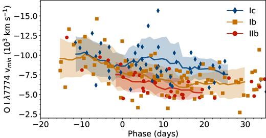
Velocity of O i λ7774 absorption minimum as a function of phase for SNe IIb, Ib, and Ic. Measures from individual spectra are shown as points, with a rolling window mean and associated standard deviations, calculated with a window size of 30 days, shown as lines and shaded regions.
4.2 Nebular emission lines
Matheson et al. (2001) examine the FWHM values of forbidden emission features in late-time stripped-envelope SN spectra. They find SNe Ic to have broader emission than SNe Ib, and they propose this to be a result of similar explosion energies but varying helium-hydrogen envelope masses across the subclasses at the time of core collapse. This data release includes a much larger set of late-time spectra – we include some 200 + spectra having a well-determined phase (see Sections 2.1 and 2.3) and observed 60 + days after peak.
To compare, we measure the FWHM of the [Ca ii] λλ7319, 7324 blended doublet, which is strong and relatively well isolated from other emission features for all subtypes of stripped-envelope SNe. [Note that this feature arises from a doublet, but only a small fraction of the observed line widths can be attributed to the 5 Å (∼200 km s−1) separation between the doublet.] We find no evidence for a systematic difference in late-time emission-line widths between SNe IIb, Ib, and Ic (see Fig. 7). Between 50 and 100 d post-peak, the measured widths for all subtypes show a wide scatter with an overall trend downward, as the SNe are transitioning into the nebular phase and the forbidden calcium emission begins to dominate the measurements, but after day 100 all three subtypes exhibit little evolution and hover around |$\rm {FWHM} \approx 200$| Å (8200 km s−1). This is in good agreement with the 8700 ± 2700 km s−1 that Matheson et al. (2001) found for the nine SNe Ic spectra in their sample, but is in disagreement with the 4900 ± 800 km s−1 they calculated from their small sample of four SNe Ib.
![The FWHM of the blended [Ca ii] λλ7319, 7324 doublet as a function of phase for SNe IIb, Ib, and Ic. Lines and shaded regions show a rolling window mean and standard deviation with window size of 50 days. We find that the three distributions overlie each other with no significant differences.](https://oup.silverchair-cdn.com/oup/backfile/Content_public/Journal/mnras/482/2/10.1093_mnras_sty2719/1/m_sty2719fig7.jpeg?Expires=1750073404&Signature=r3jH6SRHQCxCncH6glM3y-vDCfCcXLWv83dsL-oXbXSmdKptxx-IU2zPndn3F59HmI25VTXOg1gic7UmSHngG3V1NPdRkEKmF6O2SbiiH5KqDpO7zAyUCI8v5HLgeiCVW4Q0Rj1L6GLmK4IeMdNBNe66a3onmry66yJ7n6-DWEmToWVpadjvwbfoVjQHCAsOwcDTJy8tGleK6YeS7tft5N6Y6xldMAXYHa~H6hzPihwb959QTs~SfkbFZFFejHMy1EhByVjA1LkhYKvUTKxOahBZ0n3ylxendx3WT~~lOquuT1TO1m7jMRT10ScQ~Xc3U4-OQ3IDFe9vYceQXY3sVw__&Key-Pair-Id=APKAIE5G5CRDK6RD3PGA)
The FWHM of the blended [Ca ii] λλ7319, 7324 doublet as a function of phase for SNe IIb, Ib, and Ic. Lines and shaded regions show a rolling window mean and standard deviation with window size of 50 days. We find that the three distributions overlie each other with no significant differences.
4.3 Helium-strength evolution
Matheson et al. (2001) find evidence for a temporal evolution in the relative strengths of helium lines in SNe Ib, with both He i λ5876 and He i λ7065 growing in strength compared to He i λ6678 after day ∼30. Liu et al. (2016), however, do not find such a trend in their pEW measures, and the data presented here do not indicate a significant trend. Fig. 8 shows the relative pEWs of these three He i lines, normalized to the He i λ6678 measure, for those SN Ib and IIb spectra having a known phase and clear simultaneous detections of all three lines. We also examine these line ratios amongst the SN Ib and SN IIb populations separately, and again find no evidence for strong temporal evolution.
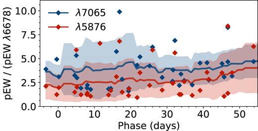
The pEW of He i λ5876 and He i λ7065 relative to that of He i λ6678, in the SN Ib and SN IIb spectra having a known phase and robust detections of all three lines. The rolling window mean and standard deviation, calculated with a window size of 20 days, is shown with lines and shaded regions (respectively). The relative strengths of these three lines are consistently ordered |$\rm {pEW}_{\lambda 5876} \gt \rm {pEW}_{\lambda 7065} \gt \rm {pEW}_{\lambda 6678}$|, but we find no significant temporal evolution in these ratios.
4.4 Mean spectra
To illustrate the spectral line variations between major subclasses over time, we construct continuum-removed mean spectra at a few phases (relative to peak) for each major spectral subtype, in much the same manner as Liu et al. (2016) and Liu, Modjaz & Bianco (2017). In detail, this process involves several steps. First we take all SNe within our sample that are classified as normal SNe IIb, Ib, or Ic and which have a date of peak brightness measurement as described in Section 2.1 or Section 2.3. We take those spectra observed within four different phase bins (each bin has a width of ±2.5 d and they are centred at −10, 0, +10, and +20 d relative to peak brightness) and choose a single spectrum per SN per bin, preferring spectra that span the entire wavelength range and those observed at a phase nearest the bin centre.
After applying redshift and Milky Way dust reddening corrections, we fit for a smooth pseudo-continuum. We then approximate each spectrum’s effective continuum with a cubic spline and we normalize the spectra by dividing each by their continuum, to allow line-strength comparisons across different SNe (which are likely affected by different amounts of host-galaxy dust reddening). We smooth the continuum-divided spectra via convolution with a window of width 21 Å and interpolate on to a single shared wavelength array. Within each binned set of SNe, we then find the mean value and standard deviation of the normalized spectra as a function of wavelength. Our results are shown in Fig. 9.
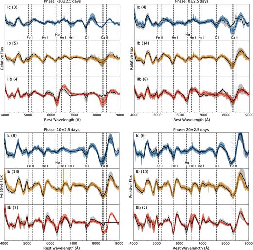
Mean spectra calculated in four different phase bins for normal members of the three dominant stripped-envelope SN subtypes. Within each bin, we include only a single spectrum per SN, and the number of SNe represented by each panel is shown in parentheses. Spectra calculated from our sample are shown in colour and those presented by Liu et al. (2016) are in grey, for comparison. Major line identifications are provided (though note that not all of these lines are visible in all SN types), and the standard deviation within the bin is illustrated by the shaded regions.
The key spectral differences between classes are readily apparent in Fig. 9. Strong H α is visible in the SN IIb spectra at all phases, but not in the SN Ib and SN Ic spectra. Strong He i lines are found in the SN Ib and SN IIb spectra, but not in the SN Ic spectra. O i is found in all, but is notably stronger in the SN Ic spectra than in the SN Ib and SN IIb spectra (see Section 4.1). Fe ii features can be found toward the blue edge for all SN types, and the near-infrared Ca ii triplet dominates their red extremes.
Previous authors (e.g. Parrent et al. 2016) have argued for the presence of weak high-velocity H α in some SNe Ib and Ic, and Liu et al. (2016) find a high-velocity feature in their mean spectra at −10 and 0 d that is reasonably interpreted to be this high-velocity hydrogen. The same feature is apparent in our SN Ib mean spectra at −10 and 0 d, just blueward of the Hα feature marked on the SN IIb spectra.
4.5 Nebular-phase spectra
At late times (≳60 d), the ejecta of stripped-envelope SNe become largely transparent and transition into the nebular phase. This data release includes a large set of spectra observed after this transition. These spectra do not show a continuum flux level against which to normalize out the effects of host-galaxy dust obscuration, as we have done with the photospheric spectra in Section 4.4, so it is difficult to perform quantitative analyses of the same sort across the entire set of observations.
Instead, in Fig. 10 we simply plot these nebular spectra overlain atop each other as an illustration of the qualitative trends in the data. It is apparent that nebular-phase spectra of the three main stripped-envelope SN subclasses are quite similar, and are dominated by the same oxygen and calcium emission features having similar strengths and line widths. While the only Hα emission found in the SN Ic and SN Ib spectra is the occasional unresolved galactic emission line, a few of the SN IIb spectra in our sample show broad nebular Hα emission associated with ongoing interaction with extended H-rich CSM (e.g. Matheson et al. 2000b).
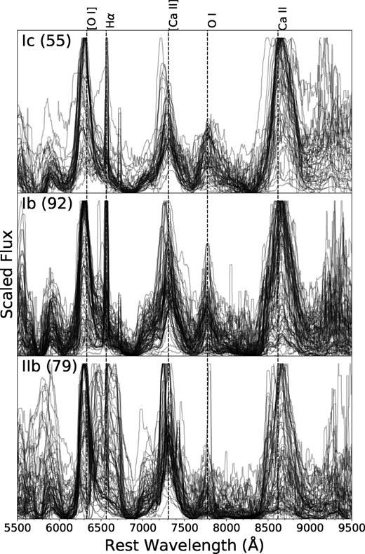
Nebular spectra of SNe Ic, Ib, and IIb are shown in the top, middle, and bottom panels (respectively). The number of spectra is listed in parentheses, and each spectrum has had a linear continuum subtracted and has been renormalized to range between 0 and 1. This format has been chosen for display purposes; the plotted minima of these spectra may differ from zero flux.
Fig. 10 may suggest a few other trends as well, though we again caution the reader that the spectra in these plots have not been corrected for host-galaxy dust obscuration, and they have been independently renormalized; we leave a detailed exploration of the nebular-phase spectra to future work.
4.6 Subpopulations of interest
Stripped-envelope SNe represent a sizeable fraction of all SNe in a volume-limited sample (∼31 per cent of core-collapse SNe are stripped-envelope; e.g. Li et al. 2011; Smith et al. 2011; Shivvers et al. 2017a), with an overall rate in good agreement with the observed population fraction of their most common progenitors (∼33 per cent of massive stars lose their outer envelope via binary interaction before core collapse; e.g. Sana et al. 2012). In addition to the ‘normal’ SNe IIb, Ib, and Ic, a diverse but relatively small set of outliers has also been discovered in the stripped-envelope SN population, exhibiting anomalous observed spectral properties, light curves, luminosities, and explosion-site locations.
Some of these outliers appear to be (in some way or another) unique amongst the as-yet-observed set of SNe, but many others are well clustered in their characteristics and form interesting subpopulations, including the superluminous SNe Ic (SLSNe Ic), the SN Ib-like SNe with strong Ca ii lines relative to O i lines (the ‘Ca-rich’ SNe), and the SNe Ib and IIb showing evidence of interaction with dense CSM (the SNe Ibn and IIbn). The progenitor channels for these relatively rare subpopulations are only poorly understood, if at all, and many puzzles about their origins remain. Here we highlight the rare subpopulation observations published as part of this sample. These subtypes are generally not well-represented in the snid template set, and so the spectral classification scheme described in Section 2.2 is not adequate – these examples were discovered and classified by hand through various methods, usually after the automatic classification workflow used for the normal events had failed, and it is difficult to assess how complete our classifications are.
A small subset of events exhibit the properties associated with the presence of very dense CSM, most notably narrow spectral emission lines arising from the ionized but not yet shock-accelerated material. These events have been dubbed SNe Ibn (‘n’ for ‘narrow lines’), following the nomenclature used for the more common SNe IIn (e.g. Schlegel 1990; Filippenko 1991; Matheson et al. 2000a; Pastorello et al. 2007). There have also been a few events that show only very weak hydrogen features, and they have been labelled SNe IIbn (e.g. Pastorello et al. 2015). Observations of several of the well-studied members of this subclass are included in this sample (much of which has already been published; e.g. SNe 2006jc and 2015G; Foley et al. 2007; Shivvers et al. 2016, 2017b), but we also include in this release several observations published here for the first time (see Fig. 11).

In addition to the SNe Ibn/IIbn, a very small set of events has appeared to be more-or-less normal SNe Ib in their spectral properties at peak brightness, but then showed strong interaction-driven hydrogen emission features at late phases (SNe 2001em, 2004dk, and 2014C; e.g. Chugai & Chevalier 2006; Milisavljevic et al. 2015; Margutti et al. 2017; Mauerhan et al. 2018). These events likely exploded inside the cavity of a dense shell of CSM lost from their progenitors in the few thousands of years before core collapse, and several examples of SNe having hydrogen-rich ejecta but similar shells of CSM have been found (e.g. SN 1996cr; Bauer et al. 2008). Though we present no new events of this nature, included in this data release are several newly published observations of both SN 2001em and SN 2014C (see Fig. 12).

Spectra of the late-interacting SNe Ib included in this release. A subset of these spectra was previously published by Mauerhan et al. (2018).
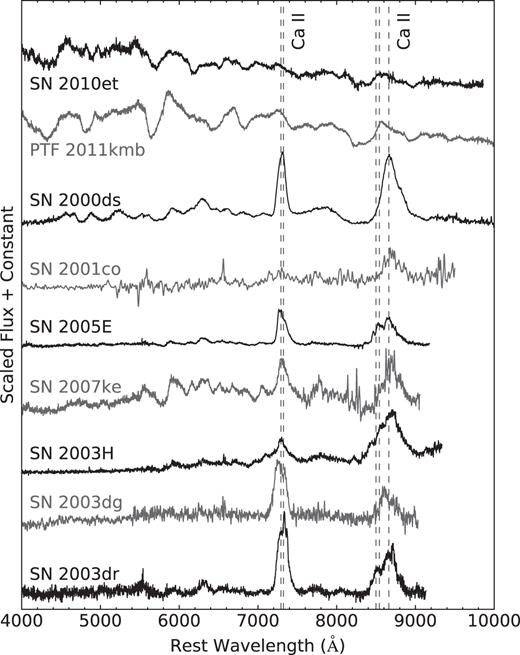
There is a population of events that spectroscopically appear to be of Type Ib at maximum brightness, yet they have relatively low luminosity, fade rapidly, exhibit peculiarly strong nebular Ca ii lines at late phases, and explode far from the strongly star-forming regions with which core-collapse events are generally associated – the ‘Ca-rich’ SNe (Filippenko et al. 2003; Perets et al. 2010). The exact progenitor channel for this subclass remains uncertain (Kasliwal et al. 2012; Foley 2015); Fig. 13 shows the Ca-rich events with data included in this release.
Finally, we also make note of the few observations of SLSNe-I included in this release. Superluminous SNe are generally an order of magnitude more luminous than normal core-collapse SNe, and they come in both hydrogen-rich (SLSNe-II) and hydrogen-poor varieties (SLSNe-I; e.g. Gal-Yam 2012; Liu et al. 2017). Energy contributions from a newly formed magnetar provide a plausible progenitor channel for these brilliant events, but many questions still remain (e.g. Dessart et al. 2012b; Inserra et al. 2013; Nicholl, Guillochon & Berger 2017); Fig. 14 shows a few of the SLSN I observations included in this release.

5 CONCLUSIONS
We present the complete sample of stripped-envelope SN spectra observed by the U.C. Berkeley SN group over the last three decades: 888 spectra of 302 SNe, including 384 spectra (of 92 SNe) with photometrically determined phases. Comparisons with previous work show that this data set proves a powerful addition to the observational study of massive stellar deaths.
We confirm previously noted trends in the O i λ7774 line properties of these events: both the strength and characteristic velocity of oxygen absorption are higher in SNe Ic than in SNe Ib and IIb at phases near peak brightness. This is best understood as evidence that the progenitors of Type Ic SNe have had their outer hydrogen and helium envelopes more heavily stripped than have those of Types Ib or IIb, and that the spectra of SNe Ic are probing more deeply into their more strongly accelerated C-O cores.
However, contrary to previous claims and somewhat at odds with the above result, we find that the line widths of late-time emission features are not a function of spectral type. We also find that the relative strengths of He i absorption lines in SNe Ib and IIb are not strongly correlated with phase, emphasizing that capturing the date of peak brightness in the light curve is of great value.
Finally, we produce continuum-removed mean spectra of SNe Ic, Ib, and IIb (which are consistent with those of Liu et al. 2016) to help define the spectral characteristics of the subclasses, and we present new observations of several categories of rare and poorly understood events. Our spectra and all associated data tables are made available online.
SUPPORTING INFORMATION
Table 2. The SNe in our sample.
Table 3. The spectra presented in this paper.
Please note: Oxford University Press is not responsible for the content or functionality of any supporting materials supplied by the authors. Any queries (other than missing material) should be directed to the corresponding author for the article.
ACKNOWLEDGEMENTS
We would like to thank Brian J. Barris, Peter Blanchard, Joshua S. Bloom, Bethany E. Cobb, Alison Coil, Louis-Benoit Desroches, Andrea Gilbert, Christopher V. Griffith, Luis C. Ho, Saurabh W. Jha, Michael T. Kandrashoff, Minkyu Kim, Nicholas Lee, Adam A. Miller, Matthew R. Moore, Aleksandir Morton, Robin E. Mostardi, Peter E. Nugent, Marina S. Papenkova, Sung Park, Daniel A. Perley, David Pooley, Dovi Poznanski, Adam G. Riess, Brad Tucker, Vivian U, XiangGao Wang, and Xiaofeng Wang for their assistance with some of the observations over the last three decades. We are grateful to the staff at Lick and Keck Observatories for their hard work in making the observations possible. Some of the data presented herein were obtained at the W. M. Keck Observatory, which is operated as a scientific partnership among the California Institute of Technology, the University of California, and the National Aeronautics and Space Administration (NASA); the observatory was made possible by the generous financial support of the W. M. Keck Foundation. The authors wish to recognize and acknowledge the very significant cultural role and reverence that the summit of Maunakea has always had within the indigenous Hawaiian community; we are most fortunate to have the opportunity to conduct observations from this mountain.
Research at Lick Observatory is partially supported by a generous gift from Google. We also greatly appreciate contributions from numerous individuals, including Charles Baxter and Jinee Tao, Firmin Berta, Marc and Cristina Bensadoun, Frank and Roberta Bliss, Eliza Brown and Hal Candee, Kathy Burck and Gilbert Mon toya, Alan and Jane Chew, David and Linda Cornfield, Michael Danylchuk, Jim and Hildy DeFrisco, William and Phyllis Draper, Luke Ellis and Laura Sawczuk, Jim Erbs and Shan Atkins, Alan Eustace and Kathy Kwan, David Friedberg, Harvey Glasser, Charles and Gretchen Gooding, Alan Gould and Diane Tokugawa, Thomas and Dana Grogan, Alan and Gladys Hoefer, Charles and Patricia Hunt, Stephen and Catherine Imbler, Adam and Rita Kablanian, Roger and Jody Lawler, Kenneth and Gloria Levy, Peter Maier, DuBose and Nancy Montgomery, Rand Morimoto and Ana Henderson, Sunil Nagaraj and Mary Katherine Stimmler, Peter and Kristan Norvig, James and Marie O’Brient, Emilie and Doug Ogden, Paul and Sandra Otellini, Jeanne and Sanford Robertson, Stanley and Miriam Schiffman, Thomas and Alison Schneider, Ajay Shah and Lata Krishnan, Alex and Irina Shubat, the Silicon Valley Community Foundation, Mary-Lou Smulders and Nicholas Hodson, Hans Spiller, Alan and Janet Stanford, the Hugh Stuart Center Charitable Trust, Clark and Sharon Winslow, Weldon and Ruth Wood, and many others. KAIT and its ongoing operation were made possible by donations from Sun Microsystems, Inc., the Hewlett-Packard Company, AutoScope Corporation, Lick Observatory, the NSF, the University of California, the Sylvia & Jim Katzman Foundation, and the TABASGO Foundation.
Support for A.V.F.’s SN research group has been provided by the National Science Foundation (NSF), the TABASGO Foundation, Gary and Cynthia Bengier, the Christopher R. Redlich Fund, and the Miller Institute for Basic Research in Science (U.C. Berkeley). A.V.F.’s work was conducted in part at the Aspen Center for Physics, which is supported by NSF grant PHY-1607611; he thanks the Center for its hospitality during the supermassive black holes workshop in June and July 2018. The U.C.S.C. group is supported in part by NSF grant AST-1518052, the Gordon & Betty Moore Foundation, the Heising-Simons Foundation, and by fellowships from the Alfred P. Sloan Foundation and the David and Lucile Packard Foundation to R.J.F. This research has made use of the NASA/IPAC Extragalactic Database (NED), which is operated by the Jet Propulsion Laboratory, California Institute of Technology, under contract with NASA.
Footnotes
iraf is distributed by the National Optical Astronomy Observatory, which is operated by the Association of Universities for Research in Astronomy, Inc., under cooperative agreement with the National Science Foundation.
Our photometry was obtained with the 0.76 -m Katzman Automatic Imaging Telescope (KAIT; Filippenko et al. 2001) at Lick Observatory and, to a much lesser degree, the Lick 1 m Nickel telescope.
REFERENCES
Author notes
Deceased 12 December 2011.
