


Abstract
We present Atacama Large Millimeter/submillimeter Array (ALMA) resolved observations of molecular gas in galaxies up to |$z$| = 0.35 to characterize the role of global galactic dynamics on the global interstellar medium properties. These observations consist of a sub-sample of 39 galaxies taken from the Valparaíso ALMA Line Emission Survey (VALES). From the CO(J = 1–0) emission line, we quantify the kinematic parameters by modelling the velocity fields. We find that the infrared (IR) luminosity increases with the rotational to dispersion velocity ratio (Vrot/σ|$v$|, corrected for inclination). We find a dependence between Vrot/σ|$v$| and the [C ii]/IR ratio, suggesting that the so-called [C ii] deficit is related to the dynamical state of the galaxies. We find that global pressure support is needed to reconcile the dynamical mass estimates with the stellar masses in our systems with low Vrot/σ|$v$| values. The star formation rate (SFR) is weakly correlated with the molecular gas fraction (|$f_{\rm H_2}$|) in our sample, suggesting that the release of gravitational energy from cold gas may not be the main energy source of the turbulent motions seen in the VALES galaxies. By defining a proxy of the ‘star formation efficiency’ (SFE) parameter as the SFR divided by the CO luminosity (SFE′ ≡ SFR/L|$^{\prime }_{\rm CO}$|), we find a constant SFE′ per crossing time (tcross). We suggest that tcross may be the controlling time-scale in which the star formation occurs in dusty |$z$| ∼ 0.03–0.35 galaxies.
1 INTRODUCTION
Star formation activity is one of the main processes that drive cosmic evolution of galaxies. Stars produce heavy elements via nucleosynthesis, which are expelled into the interstellar medium (ISM) during the late stages of their evolution, enriching the gas with metals and dust (see e.g. Nozawa & Kozasa 2013). Thus, star formation is directly involved in the processes of growth and evolution of galaxies, to the formation of planets through cosmic time. Nevertheless, our knowledge about the physical processes that dominate the formation of stars starting from pristine gas is far from complete, mainly because of the wide range of physical processes that are involved.
Schmidt (1959) was the first to propose a power-law relationship between the star formation activity of galaxies and their gas content. This relationship was later confirmed by Kennicutt (1998a,b), who revealed a clear relationship between the disc-averaged total galaxy gas (atomic plus molecular) surface density (Σgas) and the star formation rate (SFR) per surface area (ΣSFR), the Kennicutt–Schmidt relationship (hereafter, KS law). The KS law describes how efficiently galaxies turn their gas into stars. It has been used to constrain theoretical models and as a critical input to numerical simulations for galaxy evolution models (e.g. Springel & Hernquist 2003; Krumholz & McKee 2005; Vogelsberger et al. 2014; Schaye et al. 2015). Using this relationship we can compute the time at which a given galaxy would convert all of its current gas mass content Mgas if it maintains its present SFR; this time-scale is called the depletion time: tdep ≡ Mgas/SFR.
Since Kennicutt's (1998a,b) work, the KS law has been tested in numerous spatially resolved surveys on local galaxies during the last decades (e.g. Wong & Blitz 2002; Kennicutt et al. 2007; Bigiel et al. 2008; Villanueva et al. 2017, hereafter V17). These surveys have allowed us to trace the SFR surface density (ΣSFR), atomic gas surface density (ΣH i), and molecular gas surface density (|$\Sigma _{\rm {H_2}}$|) and study how these quantities relate to each other (e.g. Leroy et al. 2008, 2013). One of the first conclusions extracted from these observations was that star formation in galaxies is more strongly correlated with |$\Sigma _{\rm {H_2}}$| than with ΣH i (especially at Σgas > 10 M⊙ pc−2), with an observed molecular gas depletion time of tdep ≈ 1–2 Gyr.
When additional data from high star-forming galaxies are included, the KS law shows an apparent bimodal behaviour where ‘discs’ and ‘starburst’ galaxies appear to fill the |$\Sigma _{\rm H_2}-\Sigma _{\rm SFR}$| plane in different loci (Daddi et al. 2010). Nevertheless, by comparing ΣSFR with |$\Sigma _{\rm H_2}$| per galaxy free-fall time (tff) and/or orbital time (torb) a single power-law relationship can be recovered (e.g. Daddi et al. 2010; Krumholz, Dekel & McKee 2012). The |$\Sigma _{\rm SFR}-\Sigma _{\rm H_2}/t_{\rm ff}$| relation can be interpreted as dependence of the star formation law on the local volume density of the gas, whilst the |$\Sigma _{\rm SFR}-\Sigma _{\rm H_2}/t_{\rm orb}$| relation suggests that the star formation law is affected by the global rotation of the galaxy. Thus, the relevant time-scale gives us critical information about the physical processes that may control the formation of stars.
However, by exploiting the Valparaíso ALMA Line Emission Survey (VALES) in the local Universe (|$z$| < 0.3; see Section 2.1), Cheng et al. (2018) showed that the bimodality seen in the KS law may also be a result of the assumptions, and thus the uncertainties behind the estimates of the molecular gas mass (|$M_{\rm H_2}$|).
The absence of an electric dipole moment in the hydrogen molecule (H2) implies that direct detections of cold H2 gas are difficult to obtain (e.g. Papadopoulos & Seaquist 1999; Bothwell et al. 2013) and tracers of the molecular gas are needed. One of the methods – and perhaps the most common one – to estimate the molecular gas content is through the carbon monoxide (12C16O; hereafter CO) line luminosity (e.g. Solomon et al. 1987; Downes & Solomon 1998; Solomon & Vanden Bout 2005; Bolatto, Wolfire & Leroy 2013) of rotational low-J transitions (e.g. J = 1–0 or J = 2–1). Because the CO emission line is generally optically thick (τCO ≈ 1), its brightness temperature (Tb) is related to the temperature of the optically thick gas sheet, not the column density of the gas. Thus the mass of the self-gravitating entity, such as a molecular cloud, is related to the emission line width, which reflects the velocity dispersion of the gas (Bolatto et al. 2013).
Assuming that the CO luminosity (|$L^{\prime }_{\rm CO}$|) of an entire galaxy comes from an ensemble of non-overlapping virialized emitting clouds, if (1) the intrinsic brightness temperature of these clouds is mostly independent of the cloud size, (2) these clouds follow the size–line width relationship (Larson 1981; Heyer et al. 2009), and (3) the clouds have a similar surface density, then the molecular gas to CO luminosity relation can be expressed as |$M_{\rm H_2}=\alpha _{\rm CO}L^{\prime }_{\rm CO}$|, where |$M_{\rm H_2}$| is defined to include the helium mass, so that |$M_{\rm H_2}=M_{\rm gas, cloud}$|, the total gas mass (hence, the virial mass) for molecular clouds (Solomon & Vanden Bout 2005) and αCO is the CO-to-H2 conversion factor. This is the so-called mist model (Dickman, Snell & Schloerb 1986). Within the Milky Way, the observed relation between virial mass and CO line luminosity for Galactic giant molecular clouds (GMCs; Solomon et al. 1987) yields αCO ≈ 4.6 M⊙ (K km s−1 pc2)−1.
Although the mist model estimates the molecular gas content successfully in the Milky Way, it overestimates the gas mass in more dynamically disrupted systems, such as ultraluminous infrared galaxies (ULIRGs; Downes & Solomon 1998). Unlike Galactic clouds or gas distributed in the disc of ‘normal’ galaxies, CO emission maps of ULIRGs show that the molecular gas is contained in dense rotating discs or rings. The CO emission may not come from individual virialized clouds but from a filled intercloud medium, so the line width is determined by the total dynamical mass (Mdyn) in the region (gas and stars). The optically thick CO line emission may trace a medium bound by the gravitational potential around the galactic centre (Downes, Solomon & Radford 1993; Solomon et al. 1997). In order to estimate the |$M_{\rm H_2}$| content from |$L^{\prime }_{\rm CO}$| in those systems a different approach is required. Downes & Solomon (1998) used kinematic and radiative transfer models to derive |$M_{\rm H_2}/L^{\prime }_{\rm CO}$| ratios in ULIRGs, where most of the CO flux is assumed to come from a warm intercloud medium. The models yield αCO ≈ 0.8 M⊙ (K km s−1 pc2)−1, a ratio that is roughly 6 times lower than the standard αCO value for the Milky Way. This αCO value is usually adopted to estimate the molecular gas content in other non-virialized environments such as galaxy mergers.
On the other hand, from numerical simulations, galaxies that have similar physical conditions have similar CO-to-H2 factors. This seems to be independent of galaxy morphology or evolutionary state. Thus, rather than bimodal distribution of ‘disc’ and ‘ULIRG’ αCO values, simulations suggest that there is a continuum of conversion values that vary with galactic environment (Narayanan et al. 2012).
Therefore, spatially resolved studies of the molecular gas content and its kinematics in galaxies are critical to understand the physical processes that determine the CO-to-H2 conversion factor and the star formation activity as these two quantities seem to be dependent on the galactic dynamics.
The construction of large samples of intermediate/high-|$z$| galaxies with direct molecular gas detections (via CO emission) has remained a challenge. Beyond the local Universe, resolved CO detections are limited to the most massive/luminous yet rare galaxies or highly magnified objects (e.g. Saintonge et al. 2013). With ALMA, we are now able to study the physical conditions of the cold molecular gas in ‘typical’ galaxies at these redshifts and test if the actual models successfully explain the characteristics of the intermediate/high-|$z$| ISM. In this paper, we use the state-of-the-art capabilities of ALMA to characterize the CO(J = 1–0) kinematics of 39 ’typical’ star-forming/mildly starburst galaxies at 0.025 < |$z$| < 0.32 drawn from VALES (V17). Combining these ALMA observations with auxiliary data (e.g. Ibar et al. 2015; Hughes et al. 2017a,b), we study how the kinematics of the cold CO(1–0) gas relate to the physical conditions of the ISM. Throughout the paper, we assume a lambda cold dark matter (ΛCDM) cosmology with ΩΛ = 0.73, |$\Omega \rm _m$| = 0.27, and H0 = 70 km s−1 Mpc−1, implying a spatial resolution, determined by the typical major axis of the synthesized beam in the VALES data of 3–4 arcsec, that corresponds to a physical scale between 2 and 17 kpc.
2 SAMPLE SELECTION AND OBSERVATIONS
2.1 VALES
The VALES sample (V17) is taken from the Herschel Astrophysical TeraHertz Large Area Survey (H-ATLAS; Eales et al. 2010; Bourne et al. 2016; Valiante et al. 2016), which is one of the largest infrared (IR) and submillimitre (submm) surveys covering ∼600 deg2 of the sky taken by the HerschelSpace Observatory (Pilbratt et al. 2010). VALES covers a redshift range of 0.02 < |$z$| < 0.35, and an IR luminosity range of L8−1000 μm ≈ 1010–12 L⊙; thus, it is an excellent galaxy sample to study the molecular gas dynamics of star-forming and ‘mildly’ starburst galaxies at low redshift.
VALES is composed of ALMA observations targeting the CO(1–0) emission line in band 3 for 67 galaxies during Cycle-1 and Cycle-2, from which 49 sources were spectroscopically detected.
We use V17’s far-infrared (FIR; 8–1000 μm) luminosities, LFIR, which were derived from the spectral energy distribution (SED) constructed with photometry from the Infrared Astronomical Satellite (IRAS; Neugebauer et al. 1984), Wide-field Infrared Survey Explorer (WISE; Wright 2010), and the Herschel Photoconductor Array Camera and Spectrometer (PACS; Poglitsch et al. 2010) and Spectral and Photometric Imaging REceiver (SPIRE; Griffin et al. 2010) instruments. By assuming a Chabrier (2003) initial mass function (IMF), the SFRs are calculated following SFR (M⊙ yr−1) = 1010 × LIR (L⊙; Kennicutt 1998b). These values are systematically higher than the rates estimated from fitting the SEDs with the Bayesian code magphys (da Cunha et al. 2008) by a factor of two. However, the two estimates are well correlated despite this systematic discrepancy (see V17 for more details).
The stellar masses (M*) for our sample were calculated by modelling the SEDs from the photometry provided by the GAMA Panchromatic Data Release (Driver et al. 2016) – in which all of our galaxies are present – in 21 bands extending from the far-ultraviolet (FUV) to the far-infrared (∼0.1–500 μm). These observed SEDs have all been modelled with the Bayesian SED-fitting code magphys and presented in V17.
The observations, data reduction, and analysis are presented in detail for the complete sample in V17, whilst the [C ii] luminosity data are presented in Ibar et al. (2015).
The analysis presented in V17 shows ALMA cubes binned at different spectral resolutions (from 20 to 100 km s−1) in order to boost the signal to noise (S/N) for spectral detectability. However, the use of low or variable spectral resolution observations to derive and/or analyse galactic kinematics may lead to erroneous conclusions (see Section 3.7). Thus, we kept the spectral resolution fixed at 20 km s−1 despite the degrading of S/N in order to minimize spectral resolution effects in our dynamical analysis.
Out of the 49 galaxies that were spectroscopically detected in CO(1–0) by V17, we find that only 39 are spectroscopically detected at a 5σ significance after fixing the spectral resolution at 20 km s−1 to all sources. We show these 39 galaxies in the SFR–M* plane in Fig. 1. Our systems sample the SFRs and stellar masses in the range of 1–84 M⊙ yr−1 and 1–15 × 1010 M⊙, respectively. We note that the galaxies with a high SFR also tend to have a high M*.
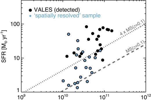
The SFR against the M* for the 39 galaxies from VALES that were spectroscopically detected at >5σ in data cubes with 20 km s−1 fixed spectral resolution (V17). In blue circles we highlight the 20 sources classified as ‘spatially resolved’ (see Section 2.1 for more details). The dashed line represents the SFR–M* relationship for ‘main-sequence’ star-forming galaxies at |$z$| = 0.1 following Genzel et al. (2015). The dotted line represents 4× the SFR value expected for a ‘main-sequence’ star-forming galaxy at a given stellar mass at |$z$| = 0.1.
Out of these 39 galaxies, 20 are considered as ‘spatially resolved’ (R) by following these criteria: (1) that the observed CO(1–0) emission extends for more than |$\sqrt{2}$| times the major axis of the synthesized beam and (2) that the observations should have been taken with a projected synthesized beam smaller than 8 kpc. The other 19 sources are classified as ‘compact’ (C). We show the corresponding galaxy classification in the top right of each CO(1–0) intensity map (Fig. A1). In the forthcoming sections of this work, in order to guarantee enough independent pixels to be fitted within each galaxy map, we just analyse and model the kinematics of the galaxies considered as ‘resolved’.
To classify our sources as ‘normal’ star-forming or starburst galaxies, we use the parametrization defined by Genzel et al. (2015) for the specific star formation rate (sSFR ≡ SFR/M*; log [sSFR(|$z$|, M*)] = −1.12 + 1.14|$z$| − 0.19|$z$|2 − (0.3 + 0.13|$z$|) × (log M* − 10.5) Gyr−1). Galaxies with | sSFR/sSFR (|$z$|, M*) | ≤ 4 are classified as ‘normal’ star-forming galaxies, whilst all galaxies with sSFR > 4 sSFR (|$z$|, M*) are labelled as ‘starburst’. We use the SFR, stellar mass, and redshift of each source to perform this classification. In Fig. 1, the dashed line shows the ‘main sequence’ of star-forming galaxies at |$z$| = 0.1. As an example, the dotted line in Fig. 1 represents our chosen sSFR criterion for galaxies at |$z$| = 0.1.
We also use V17’s morphological classification scheme to assume a bimodal CO-to-H2 conversion factor of 0.8 or 4.6 M⊙ (K km s−1 pc2)−1 depending on whether a galaxy is classified as a ‘merger’ or ‘disc’, respectively. This classification is based on visual inspection of the galaxy images extracted by using the GAMA Panchromatic Swarp Imager tool.1 We note that in our ‘resolved’ sample, just three galaxies (HATLASJ084630.7+005055, HATLASJ085748.0+004641, and HATLASJ090750.0+010141) are classified as ‘mergers’ by the morphological criterion. We do not attempt to perform a kinematic classification of mergers (e.g. Shapiro et al. 2008; Förster Schreiber et al. 2009; Swinbank et al. 2012a; Molina et al. 2017) given that our low spatial resolution tends to smooth the emission and kinematic deviations, making galaxy intensity and velocity fields appear more discy than they actually are (Bellocchi, Arribas & Colina 2012).
The mean molecular gas fraction [|$f_{\rm H_2}\equiv M_{\rm H_2}/(M_{\rm H_2}+M_*)$|] of the ‘resolved’ sample is 0.22 within a range of 0.06–0.44 with a typical relative error for each measurement of ∼12 per cent.
2.2 Galaxy dynamics
To measure the dynamics of each galaxy, we fit the CO(1–0) emission line (νrest = 115.271 GHz) following the approach presented in Swinbank et al. (2012a). We use a χ2 minimization procedure, estimating the noise per spectral channel from a surrounding area that does not contain source emission. For a given pixel, we first attempt to identify a CO(1–0) emission line within a squared region that contains the synthesized beam size around that pixel and we take the average spectrum within that region.
Then, we fit a Gaussian profile to the spectrum and we impose an S/N > 5 threshold to the best fit to detect the emission line. If this criterion is not fulfilled, then the squared region around that pixel is increased by one pixel per side and we search for any emission line again. After this iteration, if the criterion is still not achieved, then we skip to the next pixel.
Considering that we have not applied any spectral filtering for imaging purposes, the fitted line widths correspond to the intrinsic line widths (no deconvolution is needed). Nevertheless, in order to consider whether an emission line is sufficiently sampled, we only take into account those fits in which the fitted line width is larger than |$\sqrt{2}$| times the channel width (≈28 km s−1; e.g. Fig. A1). The spectral resolution is therefore impeding narrower velocity dispersion measurements. We caution that this masking procedure may lead to an overestimated average velocity dispersion value for each galaxy.
3 METHODS
3.1 GAMA’s morphological models
With the advent of multiple integral field spectroscopy (IFS) surveys at high redshift (e.g. Förster Schreiber et al. 2009; Wisnioski et al. 2015; Stott et al. 2016), kinematic models have experienced rapid development and are becoming more complex by taking into account multiple galaxy components and adding multiple degrees of freedom (e.g. Swinbank et al. 2017). The latter increases the parameter degeneracy, especially regarding inclination angle when low spatially resolved observations are analysed. Thus, additional information must be considered in order to derive robust kinematic parameters from the observed velocity fields. With the aim to minimize parameter degeneracy, we supported our kinematic analysis by taking into account previous Sérsic photometry models (Sérsic 1963) available for the GAMA survey data (Table 1; Liske et al. 2015). Those models are produced by using sigma (Structural Investigation of Galaxies via Model Analysis; Kelvin et al. 2012) on Sloan Digital Sky Survey (SDSS) and UKIRT Infrared Deep Sky Survey (UKIDSS) imaging data. We use the K-band image models to characterize the stellar component of each galaxy through the half-light radius (r1/2,K), the orientation of the major axis indicated by the position angle (PAK), and the inclination angle derived from the minor to major axis ratio (b/a). We use this inclination value to constrain the galactic inclination of the molecular gas content in the kinematic modelling. We note, however, that the error estimates produced by sigma are determined from the covariance matrix used in the fitting procedure. As a result, the uncertainty of the inclination value tends to be underestimated (Häußler et al. 2007; Bruce et al. 2012). Therefore, we adopt a more reasonable error to the galactic inclination and discuss its choice in the following sub-section. Out of the 20 resolved galaxies analysed in this work, 19 sources have this morphological GAMA modelling. We do not use the inclination value derived for HATLASJ085836.0+013149 from its morphological model as it implies an unrealistic central surface brightness magnitude value of −18 mag arcsec−2. This galaxy was analysed without a constraint on the kinematic parameters.
GAMA’s morphological K-band photometric parameters for the ‘resolved’ galaxy sub-sample from VALES. μ0,K is the central surface brightness value. r1/2,K and nS are the half-light radius and the Sérsic photometric index, respectively. PAK is the position angle of the major axis. The ellipticity ‘e’ is derived from the semi-major and minor axis ratio (e ≡ 1 − b/a). The chi-square of the best two-dimensional fitted photometric model is given in the last column (see Section 3.1 for more details).
| K-band broad-band properties | ||||||
|---|---|---|---|---|---|---|
| ID | μ0,K | r1/2,K | nS | PAK | e | |$\chi ^2_\nu$| |
| mag arcsec−2 | arcsec | deg | ||||
| (1) | (2) | (3) | (4) | (5) | (6) | (7) |
| HATLASJ083601.5+002617 | 15.5 | 5.09 | 1.93 | 2.1 | 0.61 | 1.09 |
| HATLASJ083745.1−005141 | 15.5 | 6.26 | 2.46 | 62.8 | 0.19 | 0.92 |
| HATLASJ084217.7+021222 | 12.3 | 0.63 | 2.47 | 168.3 | 0.22 | 0.54 |
| HATLASJ084350.7+005535 | 13.5 | 1.38 | 2.61 | 0.0 | 0.57 | 1.12 |
| HATLASJ084428.3+020349 | 4.2 | 23.49 | 8.92 | 101.1 | 0.38 | 1.57 |
| HATLASJ084428.3+020657 | 15.6 | 2.04 | 1.28 | 58.6 | 0.77 | 1.63 |
| HATLASJ084630.7+005055 | 0.6 | 0.67 | 8.44 | 141.5 | 0.19 | 1.05 |
| HATLASJ084907.0−005139 | 9.7 | 1.06 | 4.95 | 136.4 | 0.34 | 1.11 |
| HATLASJ085111.5+013006 | 11.6 | 5.20 | 3.82 | 114.8 | 0.77 | 1.42 |
| HATLASJ085112.9+010342 | 13.6 | 2.68 | 2.82 | 115.6 | 0.53 | 1.16 |
| HATLASJ085340.7+013348 | 16.9 | 6.68 | 2.18 | 27.4 | 0.13 | 1.17 |
| HATLASJ085346.4+001252 | 14.9 | 3.31 | 1.93 | 46.0 | 0.77 | 1.07 |
| HATLASJ085356.5+001256 | 17.8 | 4.56 | 1.56 | 57.4 | 0.29 | 1.08 |
| HATLASJ085450.2+021207 | 14.0 | 3.62 | 2.58 | 150.3 | 0.52 | 1.48 |
| HATLASJ085616.0+005237 | 13.9 | 0.97 | 2.54 | 78.1 | 0.10 | 1.05 |
| HATLASJ085748.0+004641 | 10.1 | 0.72 | 3.48 | 125.3 | 0.10 | 1.28 |
| HATLASJ085828.5+003815 | 8.8 | 7.51 | 5.93 | 121.0 | 0.25 | 1.19 |
| HATLASJ085836.0+013149 | – | – | – | – | – | – |
| HATLASJ090004.9+000447 | 12.5 | 1.85 | 2.84 | 47.6 | 0.22 | 1.47 |
| HATLASJ090750.0+010141 | 8.2 | 1.49 | 5.40 | 66.3 | 0.28 | 1.89 |
| HATLASJ091205.8+002655 | 9.8 | 0.97 | 4.04 | 52.2 | 0.07 | 1.24 |
3.2 Inclination angles
3.3 Kinematic model
We attempt to model the two-dimensional velocity field by first identifying the dynamical centre and the kinematic major axis. Considering the modest spatial resolution of our observations and the smoothness of the intensity maps, we constrain the kinematic centre to the CO(1–0) intensity peak location. We follow Swinbank et al. (2012a) to construct two-dimensional models with an input rotation curve following an arctan function [|$V(r)=\frac{2}{\pi }V_{\rm asym}$|arctan(r/rt)], where Vasym is the asymptotic rotational velocity and rt is the effective radius at which the rotation curve turns over (Courteau 1997). This model has four free parameters [Vasym, rt, position angle (PA), and disc inclination] and a genetic algorithm (Charbonneau 1995) is used to find the best fit (see Swinbank et al. 2012a for more details). The parameter uncertainties are calculated by considering a confidence limit of |$\Delta \chi _\nu ^2=1$|. An example of the best-fitting kinematic maps and velocity residuals is shown in Fig. 2, whilst the full sample maps are presented in the appendix (Fig. A1). The best-fitting inclination values are given in Table 2. The mean deviation from the best-fitting models within the sample (indicated by the typical r.m.s) is 〈data − model 〉 = 17 ± 9 km s−1 with a range of 〈data − model 〉 = 7–48 km s−1. We show this value for each galaxy in its residual map.
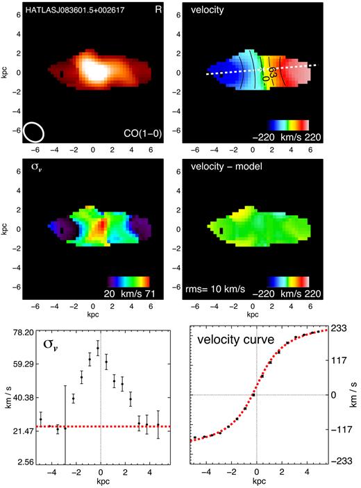
Example of the two-dimensional maps and one-dimensional velocity profiles for one target within our survey. The full sample maps, profile figures, and their explanation are shown in the appendix (Fig. A1). Left: from top to bottom, CO(1–0) intensity map, LOS velocity dispersion map, and one-dimensional velocity dispersion profile. Right: from top to bottom, rotational velocity map, residual map, and one-dimensional rotational velocity profile.
Properties of the galaxies with resolved emission from VALES. The FIR luminosities are calculated across the 8–1000 μm wavelength range. θFWHM is the synthesized beam major axis size. The CO(1–0) half-light radii (|$r_{1/2, \rm CO}$|) are deconvolved by the synthesized beam. The inclination angle is defined as the angle between the LOS and the plane perpendicular to the galactic disc (for a face-on galaxy, inc = 0 deg). σ|$v$| is the median velocity dispersion corrected for ‘beam smearing’ effects; see Section 3.6. Vrot is the rotational velocity at 2 times the CO(1–0) half-light radius corrected for inclination. |$\chi ^2_\nu$| is the reduced chi-square of the best two-dimensional fit. The galaxy classification in the final column denotes ‘Resolved’ (R) or ‘Compact’ (C) (see Section 2.1 for more details).
| Galaxy Properties | ||||||||||||||
|---|---|---|---|---|---|---|---|---|---|---|---|---|---|---|
| HATLAS-DR1 ID | RA | Dec. | |$z$|spec | logM⋆ | logLFIR | |$L_{\rm {[C\, {\small II}]}}$| | |$L^{\prime }_{\rm {CO}}$| | θFWHM | |$r_{1/2,\rm CO}$| | inc | σ|$v$| | Vrot | |$\chi ^2_\nu$| | Class. |
| J2000 | J2000 | M⊙ | L⊙ | ×108 L⊙ | ×1010 L⊙ | kpc | kpc | deg | km s−1 | km s−1 | ||||
| (1) | (2) | (3) | (4) | (5) | (6) | (7) | (8) | (9) | (10) | (11) | (12) | (13) | (14) | (15) |
| HATLASJ083601.5+002617 | 08:36:01.6 | +00:26:18.1 | 0.03322 | 10.59 ± 0.1 | 10.31 ± 0.02 | 0.97 ± 0.02 | 0.104 ± 0.004 | 2.22 | 3.4 ± 0.1 | 80.8 ± 0.1 | 24 ± 2 | 180 ± 3 | 0.13 | R |
| HATLASJ083745.1−005141 | 08:37:45.2 | −00:51:40.9 | 0.03059 | 10.35 ± 0.1 | 10.13 ± 0.03 | 0.73 ± 0.01 | 0.034 ± 0.003 | 2.06 | 4.4 ± 0.3 | 57.2 ± 0.1 | 25 ± 1 | 115 ± 1 | 0.14 | R |
| HATLASJ083831.9+000045 | 08:38:31.9 | +00:00:45.0 | 0.07806 | 10.27 ± 0.1 | 11.15 ± 0.01 | 2.43 ± 0.10 | 0.250 ± 0.019 | 6.05 | – | – | – | – | – | C |
| HATLASJ084217.7+021222 | 08:42:17.9 | +02:12:23.4 | 0.09602 | 10.53 ± 0.1 | 10.93 ± 0.04 | 2.28 ± 0.11 | 0.249 ± 0.020 | 5.58 | 12.0 ± 3.1 | 77.5 ± 0.2 | 35 ± 7 | 75 ± 3 | 0.16 | R |
| HATLASJ084305.0+010858 | 08:43:05.1 | +01:08:56.0 | 0.07770 | 10.41 ± 0.2 | 11.05 ± 0.03 | – | 0.166 ± 0.017 | 6.13 | – | – | – | – | – | C |
| HATLASJ084350.7+005535 | 08:43:50.8 | +00:55:34.8 | 0.07294 | 10.64 ± 0.1 | 11.03 ± 0.01 | 1.70 ± 0.09 | 0.191 ± 0.016 | 5.52 | 4.2 ± 0.3 | 67.3 ± 0.7 | 70 ± 8 | 58 ± 3 | 0.71 | R |
| HATLASJ084428.3+020349 | 08:44:28.4 | +02:03:49.8 | 0.02538 | 10.29 ± 0.1 | 10.25 ± 0.01 | 0.33 ± 0.01 | 0.041 ± 0.003 | 1.76 | 2.4 ± 0.4 | 80.0 ± 0.2 | 59 ± 14 | 69 ± 6 | 0.86 | R |
| HATLASJ084428.3+020657 | 08:44:28.4 | +02:06:57.4 | 0.07864 | 10.78 ± 0.1 | 11.01 ± 0.03 | 4.51 ± 0.14 | 0.392 ± 0.051 | 6.22 | 6.3 ± 0.5 | 83.5 ± 0.2 | 39 ± 2 | 162 ± 3 | 2.50 | R |
| HATLASJ084630.7+005055 | 08:46:30.9 | +00:50:53.3 | 0.13232 | 10.36 ± 0.1 | 11.51 ± 0.02 | 6.22 ± 0.63 | 0.463 ± 0.042 | 7.51 | 4.5 ± 0.5 | 33.3 ± 0.1 | 37 ± 28 | 215 ± 8 | 20.6 | R |
| HATLASJ084907.0−005139 | 08:49:07.1 | −00:51:37.7 | 0.06979 | 10.48 ± 0.1 | 11.18 ± 0.01 | 2.28 ± 0.09 | 0.279 ± 0.022 | 5.27 | 4.7 ± 1.3 | 45.9 ± 0.3 | 54 ± 3 | 108 ± 4 | 0.33 | R |
| HATLASJ085111.5+013006 | 08:51:11.4 | +01:30:06.9 | 0.05937 | 10.56 ± 0.1 | 10.72 ± 0.02 | 2.66 ± 0.07 | 0.198 ± 0.007 | 4.63 | 6.5 ± 0.4 | 76.2 ± 0.1 | 31 ± 8 | 207 ± 4 | 0.22 | R |
| HATLASJ085112.9+010342 | 08:51:12.8 | +01:03:43.7 | 0.02669 | 10.14 ± 0.1 | 10.20 ± 0.01 | 0.24 ± 0.01 | 0.020 ± 0.003 | 1.85 | 1.1 ± 0.3 | 58.0 ± 0.9 | 43 ± 19 | 81 ± 4 | 0.74 | R |
| HATLASJ085234.4+013419 | 08:52:33.9 | +01:34:22.7 | 0.19500 | 10.57 ± 0.1 | 11.92 ± 0.01 | – | 1.999 ± 0.012 | 14.9 | – | – | – | – | – | C |
| HATLASJ085340.7+013348 | 08:53:40.7 | +01:33:47.9 | 0.04101 | 10.36 ± 0.1 | 10.28 ± 0.03 | 0.95 ± 0.02 | 0.061 ± 0.003 | 2.95 | 3.6 ± 0.3 | 39.0 ± 0.2 | 24 ± 3 | 181 ± 14 | 0.13 | R |
| HATLASJ085346.4+001252 | 08:53:46.3 | +00:12:52.4 | 0.05044 | 10.31 ± 0.1 | 10.71 ± 0.01 | 2.18 ± 0.04 | 0.076 ± 0.002 | 3.57 | 6.4 ± 0.4 | 89.7 ± 0.2 | 33 ± 5 | 134 ± 4 | 0.26 | R |
| HATLASJ085356.5+001256 | 08:53:56.3 | +00:12:56.3 | 0.05084 | 10.01 ± 0.1 | 10.33 ± 0.03 | 1.41 ± 0.04 | 0.068 ± 0.002 | 3.60 | 2.6 ± 0.2 | 52.2 ± 0.1 | 25 ± 4 | 109 ± 2 | 0.14 | R |
| HATLASJ085450.2+021207 | 08:54:50.2 | +02:12:08.3 | 0.05831 | 10.66 ± 0.1 | 10.70 ± 0.02 | 2.30 ± 0.08 | 0.202 ± 0.019 | 4.66 | 3.9 ± 0.1 | 70.4 ± 0.1 | 39 ± 16 | 287 ± 6 | 1.52 | R |
| HATLASJ085616.0+005237 | 08:56:16.0 | +00:52:36.2 | 0.16916 | 10.96 ± 0.1 | 10.94 ± 0.01 | – | 0.443 ± 0.076 | 10.4 | – | – | – | – | – | C |
| HATLASJ085748.0+004641 | 08:57:48.0 | +00:46:38.7 | 0.07177 | 10.37 ± 0.1 | 11.27 ± 0.01 | 4.69 ± 0.09 | 0.276 ± 0.014 | 5.57 | 4.6 ± 0.3 | 70.2 ± 0.1 | 51 ± 5 | 43 ± 3 | 0.10 | R |
| HATLASJ085828.5+003815 | 08:58:28.6 | +00:38:14.8 | 0.05236 | 10.43 ± 0.1 | 10.44 ± 0.02 | 0.94 ± 0.03 | 0.043 ± 0.005 | 3.72 | 2.6 ± 0.2 | 52.3 ± 0.1 | 22 ± 2 | 159 ± 2 | 0.16 | R |
| HATLASJ085836.0+013149 | 08:58:36.0 | +01:31:49.0 | 0.10677 | 10.90 ± 0.1 | 11.22 ± 0.01 | 5.30 ± 0.21 | 0.554 ± 0.011 | 6.17 | 11.1 ± 0.8 | 80.0 ± 0.1 | 27 ± 4 | 91 ± 1 | 0.19 | R |
| HATLASJ090004.9+000447 | 09:00:05.0 | +00:04:46.8 | 0.05386 | 10.70 ± 0.1 | 10.57 ± 0.02 | 1.86 ± 0.06 | 0.153 ± 0.022 | 3.80 | 2.7 ± 0.1 | 42.5 ± 0.2 | 25 ± 2 | 193 ± 10 | 0.22 | R |
| HATLASJ090750.0+010141 | 09:07:50.1 | +01:01:41.8 | 0.12808 | 10.14 ± 0.1 | 11.70 ± 0.01 | 9.33 ± 0.40 | 0.535 ± 0.045 | 7.36 | 10.3 ± 0.6 | 44.8 ± 1.4 | 58 ± 6 | 35 ± 5 | 0.12 | R |
| HATLASJ090949.6+014847 | 09:09:49.6 | +01:48:46.0 | 0.18186 | 10.89 ± 0.1 | 11.84 ± 0.02 | 13.8 ± 0.68 | 1.364 ± 0.093 | 12.7 | – | – | – | – | – | C |
| HATLASJ091157.2+014453 | 09:11:57.2 | +01:44:53.9 | 0.16945 | 10.90 ± 0.2 | 11.39 ± 0.01 | – | 0.737 ± 0.072 | 11.0 | – | – | – | – | – | C |
| HATLASJ091205.8+002655 | 09:12:05.8 | +00:26:55.6 | 0.05446 | 10.33 ± 0.1 | 11.09 ± 0.01 | 1.45 ± 0.05 | 0.187 ± 0.011 | 3.94 | 2.6 ± 0.3 | 21.0 ± 0.5 | 79 ± 24 | 116 ± 12 | 0.11 | R |
| HATLASJ091420.0+000509 | 09:14:20.0 | +00:05:10.0 | 0.20216 | 10.62 ± 0.1 | 11.55 ± 0.01 | – | 0.667 ± 0.114 | 13.0 | – | – | – | – | – | C |
| HATLASJ091956.9+013852 | 09:19:57.0 | +01:38:51.6 | 0.17635 | 10.45 ± 0.1 | 11.13 ± 0.01 | – | 0.365 ± 0.048 | 11.7 | – | – | – | – | – | C |
| HATLASJ113858.4−001629 | 11:38:58.5 | −00:16:30.2 | 0.16370 | 10.84 ± 0.1 | 11.21 ± 0.01 | – | 0.546 ± 0.129 | 8.94 | – | – | – | – | – | C |
| HATLASJ114343.9+000203 | 11:43:44.1 | +00:02:02.5 | 0.18716 | 10.10 ± 0.1 | 11.05 ± 0.01 | – | 0.485 ± 0.089 | 10.1 | – | – | – | – | – | C |
| HATLASJ114625.0−014511 | 11:46:25.0 | −01:45:13.0 | 0.16450 | 10.72 ± 0.1 | 11.72 ± 0.01 | – | 0.861 ± 0.084 | 8.91 | – | – | – | – | – | C |
| HATLASJ121141.8−015730 | 12:11:41.8 | −01:57:29.7 | 0.31704 | 11.18 ± 0.1 | 11.80 ± 0.01 | – | 0.210 | 15.1 | – | – | – | – | – | C |
| HATLASJ121253.5−002203 | 12:12:53.5 | −00:22:04.4 | 0.18548 | 10.79 ± 0.1 | 11.11 ± 0.01 | – | 0.447 ± 0.065 | 9.71 | – | – | – | – | – | C |
| HATLASJ121427.3+005819 | 12:14:27.4 | +00:58:18.3 | 0.18045 | 10.93 ± 0.1 | 11.27 ± 0.01 | – | 0.460 ± 0.069 | 9.63 | – | – | – | – | – | C |
| HATLASJ121446.4−011155 | 12:14:46.5 | −01:11:55.6 | 0.17971 | 10.82 ± 0.1 | 11.55 ± 0.01 | – | 0.765 ± 0.094 | 9.45 | – | – | – | – | – | C |
| HATLASJ140912.3−013454 | 14:09:12.5 | −01:34:54.9 | 0.26492 | 10.97 ± 0.1 | 11.89 ± 0.01 | – | 1.494 ± 0.231 | 9.17 | – | – | – | – | – | C |
| HATLASJ141008.0+005106 | 14:10:08.0 | +00:51:06.9 | 0.25641 | 11.10 ± 0.1 | 11.83 ± 0.01 | – | 1.311 ± 0.295 | 8.80 | – | – | – | – | – | C |
| HATLASJ142057.9+015233 | 14:20:58.0 | +01:52:32.1 | 0.26462 | 10.86 ± 0.1 | 11.64 ± 0.01 | – | 1.238 ± 0.231 | 9.55 | – | – | – | – | – | C |
| HATLASJ142517.1+010546 | 14:25:17.1 | +01:05:46.6 | 0.28069 | 11.07 ± 0.1 | 11.84 ± 0.01 | – | 1.714 ± 0.237 | 9.98 | – | – | – | – | – | C |
3.4 CO(1–0) spatial extent
To measure the spatial extent of the molecular gas of each galaxy, we calculate the CO half-light radii (|$r_{1/2,\rm CO}$|). These are calculated from the cubes, where the encircled CO(1–0) flux decays to half its total integrated value. The total integrated value is defined as the total CO(1–0) luminosity within a Petrosian radius. We adopted the SDSS Petrosian radius definition with RP,lim = 0.2. We account for the ellipticity and position angle of the galaxy obtained from the best-fitting disc model. The |$r_{1/2,\rm CO}$| 1 σ errors are derived by bootstrapping via Monte Carlo simulations in both measured emission-line intensity and estimated dynamical parameters. The half-light radii are corrected for beam-smearing effects by subtracting the synthesized beam major axis width in quadrature. The median |$r_{1/2,\rm CO}$| for our sample is 4.4 ± 3 kpc (Table 2).
3.5 Rotation curve and rotational velocity
We use the dynamical centre and position angle derived from the best-fitting dynamical model to extract the one-dimensional rotation curve across the major kinematic axis of each galaxy. An example of the extracted rotational curves is presented in Fig. 2, whilst the rotational curves for all of the sample are shown in the appendix (Fig. A1). We define the rotational velocity corrected for inclination (Vrot) as the velocity observed at two half-light radii. We note, however, that we are observing the CO(1–0) emission line; thus, the radius at which we are defining the representative rotational velocity of each source may not be directly related to the radius at which, for example, IFS surveys might extract rotational velocities using ionized gas dynamics (e.g. Förster Schreiber et al. 2009; Swinbank et al. 2012a; Green et al. 2014; Wisnioski et al. 2015; Stott et al. 2016).
3.6 Velocity gradient correction and velocity dispersion
As a consequence of the modest spatial resolution of our observations compared to the angular extension of the sources, there is a contribution to the derived line widths from the beam-smeared large-scale velocity motions across the galaxy, which must be corrected for (Davies et al. 2011). This correction is done for each pixel where the CO(1–0) emission is detected. We calculate the luminosity-weighted velocity gradient across the synthesized beam (ΔV/ΔR) in the model velocity field and we subtract it linearly from the corresponding velocity dispersion value following equation (A1) from Stott et al. (2016). However, by using this procedure, ∼20 per cent of residuals are expected to remain, especially in the centre of each galaxy where large velocity gradients are expected to be present (Stott et al. 2016).
In order to minimize the residual beam-smearing effects in our sample, we define the global velocity dispersion value (σ|$v$|) for each galaxy as the median value of the pixels at an angular distance 2 times greater than the angular extension of the synthesized beam from the best-fitted dynamical centre. This procedure usually calculates σ|$v$| by considering 71 pixels on average with a range of 6–256 pixels. In the case of HATLASJ083601.5+002617 we increased the skipped area to 3 times the synthesized beam size as our method failed due to the high galaxy inclination angle (∼80 deg) plus a beam size not large enough to avoid the zone where velocity gradients were contributing to the emission line widths.
While the CO(1–0) emission line width has been traditionally used as a measure of the dynamical mass within a GMC (e.g. Solomon et al. 1987), the synthesized beam size (2–8 kpc) within our sample is larger than the biggest GMC size observed in galaxies (∼1 kpc; e.g. Swinbank et al. 2012b), resulting in the smoothness of our galactic intensity maps (Fig. A1). Thus, throughout our work, we interpret the CO(1–0) emission line width as a tracer of the molecular gas random motions seen over a resolution element area. This is the key property of our ‘resolved’ sample as we can study the dynamics of the molecular gas directly. This opens a window of dynamical analyses that are not necessarily the same as those performed in IFS galaxy surveys, which use (mainly) the ionized gas to characterize the dynamical state of galaxies.
3.7 Spatial and spectral resolutions effects
In order to estimate the effect of the spatial and spectral resolution for the VALES sample on the kinematic parameters, we use ALMA Band-3 observations with a higher resolution of ∼ 0|${^{\prime\prime}_{.}}$|5 (∼ kpc scale at z |$\, \sim \, 0.1-0.2$|) and 12 km s−1 towards three VALES galaxies (Ibar et al. in prep.). The high resolution of those observations allows us to study in detail how spectral resolution and beam-smearing effects affect the derived kinematic parameters.
We create mock observations by spatially degrading the images using two-dimensional Gaussian kernel, while also rebinning the spectral channels to mimic lower spectral resolutions. The channel width is increased by 12 km s−1 per step between ∼12 and 84 km s−1, whilst the spatial resolution is degraded by 1 kpc per step between ∼1 and 7 kpc (up to ∼3 times the ‘fiducial’ half-light radius). From those mock data cubes we fit the CO(1–0) emission line and we derive its best-fitting kinematic model and calculate the Vrot, σ|$v$|, and |$r_{1/2, \rm CO}$| following the procedures described in the previous sections, but we keep the position angle fixed to the value obtained for the data cube with higher spatial and spectral resolutions. In Fig. 3 we show how the fitted kinematic parameters (rows) depend on the spectral resolution (left column) at a fixed ∼1 kpc scale and the spatial resolution (right column) at a fixed 12 km s−1 for the three sources. We consider the ‘fiducial’ value of each kinematic parameter for each source as the values derived for the data cubes with higher spectral and spatial resolutions (12 km s−1 and ∼1 kpc), and are represented by the horizontal dashed lines in each plot. The fiducial values for the three galaxies are Vrot = 56, 200, and 226 km s−1; σ|$v$| = 54, 53, and 76 km s−1; and |$r_{1/2,\rm CO}=$| 1.2, 4.2, and 4.6 kpc.
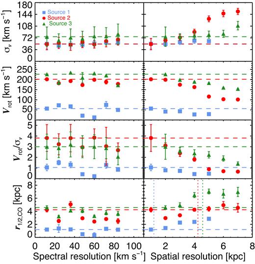
Velocity dispersion, rotational velocity, rotational velocity to velocity dispersion ratio (Vrot/σ|$v$|), and CO(1–0) intensity half-light radius (rows) as a function of the spectral and spatial resolution (columns). Those values were derived from mock data cubes produced by the convolution of a three-dimensional Gaussian kernel with the original observations. The spatial resolution corresponds to the projected major axis (full width at half-maximum, FWHM) of the synthesized beam. The blue, red, and green horizontal dashed lines represent the kinematic ‘fiducial’ values for each source. The blue, red, and green vertical dotted lines represent the ‘fiducial’ |$r_{1/2,\rm CO}$| values for each galaxy (see Section 3.7 for more details).
In Fig. 3, we see how the measured galactic velocity dispersion remains constant when the spectral resolution is degraded. We also see an increase of the velocity dispersion when we spatially degrade the cubes; however, we note that the galaxy with the lowest ‘fiducial’ rotational velocity value is also the galaxy less affected by spatial resolution effect. This is consistent with the picture in which the velocity gradient within the beam area contributes to the emission line width represented by the velocity dispersion. We note also that galaxy mass and inclination may also affect the σ|$v$| estimation (e.g. Burkert et al. 2016).
In the second row of Fig. 3 we measure Vrot for each data cube. Although we can recover nearly the same Vrot value regardless of the spectral resolution, we can see how it varies when we spatially degrade the cubes. At poor spatial resolution, lower rotational velocity values are recovered. This effect is expected as the observed emission line is the result of the convolution of the emission lines produced within the beam area. This convolution favours brighter emission lines, which are mainly produced in the central part of the galaxy where Vrot is lower.
In the third row of Fig. 3 we show the variation of the Vrot/σ|$v$| ratio as a function of spectral and spatial resolution. We see how this ratio is not affected by the increase of the channel width. However, we observe a decrease of the Vrot/σ|$v$| ratio with lower spatial resolution. This is produced by a combination of both effects, the underestimation and overestimation of the Vrot and σ|$v$| values, respectively. However, the way in which the Vrot/σ|$v$| ratio decreases seems to be different for each target, suggesting that the internal kinematics of each galaxy may affect the derived Vrot/σ|$v$| ratio through the convolution with the synthesized beam.
In the fourth row of Fig. 3 we see how |$r_{1/2,\rm CO}$| does not vary significantly with spectral resolution in any source. The gain of flux from the outskirts of each target seems to be marginal compared to the total flux of the source. On the other hand, we see a clear increase of |$r_{1/2,\rm CO}$| when we lower the spatial resolution. We note that the derived half-light radii tend to suffer an appreciable increase of their value when the synthesized beam size becomes comparable to the ‘fiducial’ |$r_{1/2,\rm CO}$| value for each galaxy (dotted vertical lines).
As a summary, the velocity dispersion and half-light radius parameters seem to be saturated to a minimum value limited by the spatial resolution. The Vrot/σ|$v$| ratio tends to decrease towards low spatial resolution. However, dispersion-dominated sources seem to be less affected by this effect. Thus, high spatial resolution data is required to obtain reliable estimates of those parameters. We find no trend between the spectral resolution and the kinematic estimates from our observations.
Taking into account the resolution effects discussed above, we set the spectral resolution to 20 km s−1, the maximum spectral resolution possible for our observations. We expect that spectral resolution effects do not strongly influence the conclusions of our work. We set this spectral resolution regardless of the spatial resolution effects inherent in our observations, which may imply an overestimation of the observed σ|$v$| and |$r_{1/2,\rm CO}$| values and an underestimation of the Vrot value for our sources.
4 RESULTS AND DISCUSSION
4.1 Morphological and kinematic properties
We show the CO(1–0) intensity, velocity, and LOS velocity dispersion maps for our sample in the appendix (Fig. A1). The intensity maps show smooth distributions of emission with no level of clumpiness except for the HATLASJ085340.7+013348 source. Despite the low-resolution data, most of our sources show a rotational pattern in their velocity maps (Fig. A1), with the larger rotational velocity values being preferentially measured in galaxies at lower |$z$|. We note that this bias effect may be mainly produced by the IR flux selection criteria used in the VALES sample (see Section 2.1). In particular, for our resolved sample, the flux criterion selects 0.02 < |$z$| < 0.2 ‘normal’ star-forming rotating disc-like galaxies, whilst it also selects 0.1 < |$z$| < 0.35 starburst galaxies with high velocity dispersion (Table 2).
We note that we find a median |$r_{1/2, K} / r_{1/2,\rm CO}$| ratio of ∼1; that is, the molecular gas component shows a spatial extension comparable to the stellar component in our galaxies. This is consistent with molecular gas observations of galaxies in the local Universe (e.g. Bolatto et al. 2017). We note that the |$r_{1/2, K} / r_{1/2,\rm CO}$| median ratio is lower than the median value (∼1.6) reported by V17 for the VALES sample. We note that this difference could be explained by considering that our emission-line fitting routine is able to find CO emission at larger radius than the V17’s procedure. Nevertheless, we calculate the CO and K-band half-light radius by taking into account the projection effects (i.e. galactic PA and inclination angles), whilst V17 do not consider such effects.
In Fig. 4 we show the distribution of Vrot, σ|$v$|, and the Vrot/σ|$v$| ratio for our resolved sample. The Vrot values range from 35 to 287 km s−1. The starburst and ‘normal’ star-forming galaxies show rotational velocities across the full range of the Vrot distribution. The velocity dispersion values range from 22 to 79 km s−1. We find median velocity dispersion values of 31 and 53 km s−1 for the ‘normal’ star-forming and starburst galaxies, respectively. However, the σ|$v$| values are susceptible to the procedure used to estimate them. Different methods can lead to inconsistent results even when the same sample is analysed (e.g. Stott et al. 2016). Thus, we perform the method developed by Wisnioski et al. (2015) to calculate the velocity dispersion values (σ|$v$|,W) in our sample and to compare with our σ|$v$| values. This method calculates the velocity dispersion values across the major axis of the galaxy, but far from the galactic centre where velocity gradients contribute to the observed line widths (see Wisnioski et al. 2015 for more details).
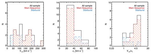
The distribution of the rotational velocity (Vrot; left), velocity dispersion (σ|$v$|; middle), and Vrot/σ|$v$| (right) within our sample. In the three panels we also show the distributions for the ‘normal’ star-forming galaxies (dashed red) and ‘starburst’ galaxies (dashed blue). This classification was done by following the same procedure adopted by V17 for VALES (see Section 2.1). Our resolved sample shows a wide range of rotation velocities and velocity dispersions.
We found a median σ|$v$|,W value of 36 km s−1, and σ|$v$|,W ranges between 19 and 70 km s−1. This median value is in agreement with the median σ|$v$| value (37 km s−1) derived by our procedure. The derived velocity dispersion ranges are also consistent for both methods. Thus, the slight overestimation of the σ|$v$| values produced by our procedure should not change the results presented in our work. We caution that we cannot neglect overestimation of velocity dispersion values produced by spatial resolution effects in this analysis.
The Vrot/σ|$v$| ratio ranges between 0.6 and 7.5, with the starburst galaxies preferential to showing the lower values. The median Vrot/σ|$v$| ratio for our sample is 4.1, and the median Vrot/σ|$v$| values for the ‘normal’ star-forming and starburst sub-samples are 4.3 and 1.6, respectively. Our sample shows a large variety of Vrot/σ|$v$| ratios, from high values comparable with those of local thin-disc galaxies (V/σ|$v$| ∼ 10–20; Bershady et al. 2010; Epinat et al. 2010), to low values comparable with the Vrot/σ|$v$| ratios observed in |$z$| ∼ 1 systems (e.g. V/σ|$v$| ∼ 2–5; Förster Schreiber et al. 2009; Wisnioski et al. 2015; Stott et al. 2016).
In Fig. 5 we study the evolution of the Vrot/σ|$v$| ratio at |$z$| = 0.10–1.0. We compare with the median Vrot/σ|$v$| values estimated for the GHASP (Epinat et al. 2010), CARMA-EDGE (Bolatto et al. 2017), DYNAMO (Green et al. 2014), KMOS3D (Wisnioski et al. 2015), and KROSS (Stott et al. 2016) surveys. The continuous line and the grey shaded area represent the best-fitting relation and the 1σ region estimated from the DEEP2 survey (Kassin et al. 2012) at |$z$| = 0.2–1.0, respectively. The dashed line represents an extrapolation of this relation at low |$z$|. DEEP2 is the only long-slit survey considered in Fig. 5. We just consider the galaxies with stellar masses between M* = 1010–11 M⊙, approximately the same stellar mass range covered by our sample (see Fig. 1). We also plot the median Vrot/σ|$v$| values for the galaxies classified as ‘starburst’ and ‘normal’ galaxies within our sample and the DYNAMO sample as both surveys study star-forming galaxies at the same epoch. However, the DYNAMO SFRs are based on dust-corrected H α emission-line measurements, whilst the SFR estimates for our sample are made by applying SED fitting. We also note that our sample and the CARMA-EDGE survey observe molecular gas kinematics, whilst the GHASP, DYNAMO, KMOS3D, and KROSS surveys study ionized gas kinematics.
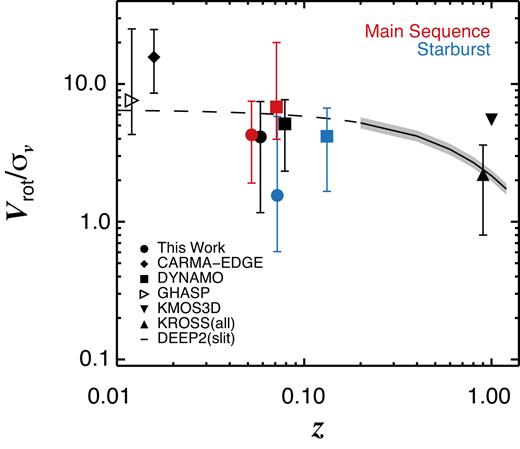
Evolution of the Vrot/σ|$v$| ratio at |$z$| ≈ 0.01–1.0. The symbols represent the median values for each survey and the error bars correspond to the 1σ region calculated from the 16th and 84th percentiles for each population. The CARMA-EDGE kinetic data are extracted by using the same procedure explained in the previous sections but assuming thin-disc geometry (see Appendix B for more details). We classify our sources and the DYNAMO galaxies as ‘starburst’ or ‘normal’ star-forming galaxy following the same procedure as that followed by V17 for VALES (see Section 2.1). The KMOS3D data correspond to the median value for ‘main-sequence’ rotationally supported star-forming disc galaxies at |$z$| ∼ 1, whilst the KROSS data correspond to the median value for the whole sample, i.e. including ‘main-sequence’ dispersion-dominated galaxies. The black line and the shaded area represent the best fit and 1σ region measured for the single-slit DEEP2 survey. The dashed line represents the extrapolation of the best fit to the DEEP2 survey data to lower redshifts.
The median Vrot/σ|$v$| value for our sample is slightly lower but still consistent with the expected value at |$z$| ∼ 0.06. This value is also comparable with the median value found for the KMOS3D sample of ‘main-sequence’ rotating-disc star-forming galaxies at |$z$| ∼ 1. However, the median Vrot/σ|$v$| value of our survey is highly influenced by the low Vrot/σ|$v$| ratios measured for our starburst galaxies (Fig. 4). If we do not consider those starburst systems, we find that the median Vrot/σ|$v$| value for the ‘normal’ star-forming galaxies in our sample is consistent with the expected value for local galaxies. It is also consistent with the median Vrot/σ|$v$| value measured for ‘normal’ star-forming galaxies within the DYNAMO survey at nearly the same epoch.
Nevertheless, the median Vrot/σ|$v$| for our starburst galaxies is ∼2.7× lower than the median value observed for the DYNAMO starburst galaxies at the same redshift, although both values are consistent within 1σ error. A difference between the spatial extension of the ionized gas compared to the molecular gas across the galaxy may explain this discrepancy. An extended ionized-gas component would allow us to measure Vrot in the flat part of the rotation curve whilst the molecular gas observations would not allow us to do it (e.g. HATLASJ084217.7+021222). On the other hand, different procedures used to calculate σ|$v$| may also explain this discrepancy. However, the different spatial resolutions at which both surveys were made are likely to be producing the discrepancy between both Vrot/σ|$v$| ratios. The DYNAMO galaxies were observed in natural seeing conditions (θFWHM = 0.9−4 arcsec), whilst our sample was observed at θFWHM = 3−4 arcsec.
Regardless of the discrepancy between the median Vrot/σ|$v$| measured for our sample and that of the DYNAMO survey, Fig. 5 shows that starburst galaxies at |$z$| ∼ 0.1–0.2 present typical Vrot/σ|$v$| values, which are consistent with the median Vrot/σ|$v$| values presented for the KMOS3D and KROSS surveys at |$z$| ∼ 1 (Wisnioski et al. 2015; Stott et al. 2016). However, high spatial resolution observations of a large sample of the low-|$z$| starburst galaxies is needed to test this result.
4.2 Luminosity dependence on galactic kinematics
4.2.1 CO(1–0) luminosity
The CO(1–0) luminosity has been widely used as an estimator of H2 mass (Bolatto et al. 2013). Through a dynamically calibrated CO-to-H2 conversion factor, reliable molecular mass estimates can be achieved (e.g. Solomon et al. 1987; Downes & Solomon 1998). Thus, depending on the dynamical model, we may expect some dependence of the CO luminosity on the galactic dynamics.
In the top panel of Fig. 6 we show the galactic |$L^{\prime }_{\rm CO}$| as a function of the rotational velocity to dispersion velocity ratio (Vrot/σ|$v$|). The Spearman rank correlation coefficient (ρSpearman) is −0.23 with a probability of 32 per cent that the correlation is produced by chance. Thus, we find a tentative weak correlation between |$L^{\prime }_{\rm CO}$| and Vrot/σ|$v$| in our data, suggesting that the CO luminosity might tend to decrease at higher Vrot/σ|$v$|. Considering that Vrot/σ|$v$| measures the level of support given by ordered versus disordered motion within a galaxy, we suggest then that turbulence-supported galaxies tend to have greater |$L^{\prime }_{\rm CO}$|.
![From top to bottom: CO(1–0), [C ii], and IR luminosities as a function of the Vrot/σ$v$ ratio for our sample. We also classify the sources as ‘starburst’ or ‘normal’ star-forming galaxy. The red open and filled diamonds represent the mean value (in log-space) for the ‘starburst’ and ‘normal’ star-forming galaxies respectively in each panel. We find a tentative anticorrelation between the LIR and the Vrot/σ$v$. Galaxies with greater pressure support, reflected by the low Vrot/σ$v$ ratio, tend to show higher CO(1–0), [C ii], and LIR luminosities. The tentative anticorrelations may suggest a smooth transition between ‘starburst’ and ‘normal’ star-forming galaxies within our VALES sample.](https://oup.silverchair-cdn.com/oup/backfile/Content_public/Journal/mnras/482/2/10.1093_mnras_sty2577/2/m_sty2577fig6.jpeg?Expires=1749956178&Signature=SRp65C~LKusIKL8g-9VjZLBk7ZswedIUH7KtYQUzRT-zvm85TieLgK2atEUZkbA2F5UJxUkhPWBg34q~WBcfpMJXyVwqNnKn5YyFxXPaZzZgN59P10Drtj3niXDQ5LmnkZOSSFfYtEiopIe~wsvhK6xpwoXYYByQPwQFB-a1hmiys7bfuR1bOEI8LddP1icY6p0UbOStf~GPLrkCbil6TX41ZgE5pC63-YQ5~ULq~81Rl74Iza6b9XVENJ1SoigkvES2zulpELgSPD1IXmJYBKMk-gPhjOiINAMO81QphI0AigKDFFzQD1S7Qw97aHhHUNpwJbI21ISv5yPu5xEPuA__&Key-Pair-Id=APKAIE5G5CRDK6RD3PGA)
From top to bottom: CO(1–0), [C ii], and IR luminosities as a function of the Vrot/σ|$v$| ratio for our sample. We also classify the sources as ‘starburst’ or ‘normal’ star-forming galaxy. The red open and filled diamonds represent the mean value (in log-space) for the ‘starburst’ and ‘normal’ star-forming galaxies respectively in each panel. We find a tentative anticorrelation between the LIR and the Vrot/σ|$v$|. Galaxies with greater pressure support, reflected by the low Vrot/σ|$v$| ratio, tend to show higher CO(1–0), [C ii], and LIR luminosities. The tentative anticorrelations may suggest a smooth transition between ‘starburst’ and ‘normal’ star-forming galaxies within our VALES sample.
The high |$L^{\prime }_{\rm CO}$| values may reflect high molecular gas masses in systems with low Vrot/σ|$v$| values. On the other hand, we may also expect that systems with high SFRs produce more UV photons which heat the gas through the photoelectric effect on dust grains. This change of gas temperature may also affect the CO-to-H2 conversion factor (Bolatto et al. 2013). However, we lack adequate observations to test this.
We also note that low Vrot/σ|$v$| ratios can be present in both disc-like galaxies and major-merger systems (Molina et al. 2017); thus, the weak correlation found in Fig. 6 suggests that the increase of the CO(1–0) luminosity may not be associated only with major merger events in agreement with previous results from numerical simulations (Shetty et al. 2011b; Narayanan et al. 2012; Papadopoulos et al. 2012). This weak correlation also suggests that turbulence may play a role in the enhancement of |$L^{\prime }_{\rm CO}$| in galaxies. Nevertheless, higher spatial resolution CO(1–0) observations are required to properly discard or validate the possible trend between CO(1–0) luminosity and Vrot/σ|$v$|.
4.2.2 [C ii] luminosity
The [C ii] λ157.74 μm emission line (νrest = 1900.54 GHz) is an FIR fine-structure line with a low ionization potential (11.26 eV) that makes it a key participant in the cooling of the warm and diffuse ISM to the cold and dense clouds (Dalgarno & McCray 1972). This emission line is a tracer of all the different stages of evolution of the ISM and detailed characterization of its emergence has been made for the Milky Way and local galaxies (e.g. Kramer et al. 2013; Pineda et al. 2013; Pineda, Langer & Goldsmith 2014) suggesting that different ISM phases produce roughly comparable contributions to the [C ii] luminosity (Madden et al. 1993). However, such detailed characterizations are impeded by observational limitations in distant galaxies that are typically detected in a single telescope beam. Thus, the [C ii] line intensity is related to an average quantity that arises from a mix of the ISM phases (e.g. Gullberg et al. 2015, and references therein). Nevertheless, physical properties of the gaseous components of the ISM may be characterized by studying correlations between the [C ii] emission and various galaxy properties [e.g. CO(1–0), LIR; Ibar et al. 2015; Hughes et al. 2017a].
In the middle panel of Fig. 6 we show the [C ii] luminosity as a function of the Vrot/σ|$v$| ratio for our galaxies. We find a weak correlation between these two quantities. We measure a ρSpearman = −0.16 with a probability of 50 per cent that the correlation is produced by chance. This may indicate that galaxies with lower Vrot/σ|$v$| values have higher [C ii] luminosity. However, we do not attempt to fit the data as we have just have two galaxies' measured [C ii] luminosity at |$L_{\rm [C\, {\small II}]}\lt 7 \times 10^7\, \mathrm{ L}_\odot$|. We need more [C ii] luminosity measurements, especially at |$L_{\rm [C\, {\small II}]}\lt 7 \times 10^7\, \mathrm{ L}_\odot$|, in order to discard or validate the possible trend between [C ii] luminosity and Vrot/σ|$v$|. [C ii] spatially resolved observations would also be useful in order to account for extended and/or nuclear emission effects (e.g. Díaz-Santos et al. 2014).
4.2.3 IR luminosity and the |$L_{[\rm C\, {\small II}]}/L_{\rm IR}$| deficit
Infrared luminosities are commonly used as a tracer of the star formation activity in galaxies. It can be understood as the emitted UV radiation from young stars that is reprocessed by dust. In the limit of complete obscuration the re-emitted LIR will effectively provide a bolometric measure of the SFR (Kennicutt 1998a). However, if the attenuation of the stellar light is not completely reprocessed, then the IR emission may underestimate the SFR. Applying SED fitting methods, the IR emission can also be used as a tracer of dust temperature (Tdust) and mass (Mdust; e.g. Draine & Li 2007; Ibar et al. 2015).
In the bottom panel of Fig. 6 we show the LIR compared to the Vrot/σ|$v$| ratio for our sources. The data present an anticorrelation with ρSpearman = −0.44 with a probability of 5 per cent that the correlation is produced by chance. Sources with greater LIR have lower Vrot/σ|$v$| values, indicating that high IR luminosities are likely to be present in systems where pressure support becomes comparable and even greater than rotational support. We note that the LIR shows stronger anticorrelation with the Vrot/σ|$v$| ratio than the CO luminosity. This suggests that the LIR/|$L^{\prime }_{\rm CO}$| ratio correlates with the Vrot/σ|$v$| values. We will discuss this further in Section 4.7.
The IR luminosity has also been traditionally compared to the [C ii] luminosity (e.g Stacey et al. 1991). The [C ii] luminosity to IR luminosity ratio (|$L_{\rm [C\, {\small II}]}/L_{\rm IR}$|) is found to be roughly constant for local star-forming galaxies with LIR < 1011 L⊙, but decreases at higher luminosities (e.g. Stacey et al. 1991; Malhotra et al. 1997). This is the so-called [C ii] deficit. However, the intricate decomposition of the [C ii] emission into the different ISM phases complicates the interpretation of this correlation (e.g. Ibar et al. 2015). Therefore, additional comparisons with other galactic properties are needed. Considering that our ‘resolved’ VALES sample covers the 1010–12 L⊙ IR luminosity range, it is an ideal sample to study the ‘[C ii] deficit’ from a kinematic point of view.
In Fig. 7 we show |$L_{\rm [C\, {\small II}]}/L_{\rm IR}$| as a function of the Vrot/σ|$v$| ratio. We find that |$L_{\rm [C\, {\small II}]}/L_{\rm IR}$| increases at high Vrot/σ|$v$| ratios but shows a significant scatter at low Vrot/σ|$v$| values. This correlation has ρSpearman = 0.76 with a probability of 0.0001 per cent that the correlation is produced by chance. We note that this probability is significantly lower than the |$L_{\rm [C\, {\small II}]}-V_{\rm rot}/\sigma _v$| and LIR – Vrot/σ|$v$| Spearman correlation probabilities. The data are well represented by a power law with a best-fitting slope of 0.74 ± 0.14. Considering that a high Vrot/σ|$v$| value suggests a host galaxy with a dominant disc geometry, our finding is consistent with that of Ibar et al. (2015), who found that galaxies presenting a prominent disc show higher |$L_{\rm [C\, {\small II}]}/L_{\rm IR}$| ratios than those that do not present discy morphologies.
![$L_{\rm [C\, {\small II}]}/L_{\rm IR}$ ratio as a function of the Vrot/σ$v$ ratio for our sample. We also classify the sources as ‘starburst’ or ‘normal’ star-forming galaxy. The dashed line represents the best power-law fit to the data and the grey shaded area represents its 1σ error. The best-fitting slope is presented in the plot. The red open and filled diamonds represent the mean value (in log-space) for the ‘starburst’ and ‘normal’ star-forming galaxies, respectively. The horizontal dotted blue line and the blue dashed area represent the median $L_{\rm [C\, {\small II}]}/L_{\rm IR}$ ratio and its 1σ region for the KINGFISH survey data regardless of the kinematics, respectively (Smith et al. 2017). We find an increase of the [C ii]/IR ratio when the Vrot/σ$v$ ratio increases.](https://oup.silverchair-cdn.com/oup/backfile/Content_public/Journal/mnras/482/2/10.1093_mnras_sty2577/2/m_sty2577fig7.jpeg?Expires=1749956178&Signature=QBqJ6rsTMWNceatAbVUTGoIBlGjMonAXxHn5lYtEGP7qDzSl1B~qFpU8kM5zGkMJ92eGu0Y3cEtaIzbbhj0RfCP2aE87F4E5BdR8AFEBUgbgB3wl9519WYMBIVsPaw9ryMPjzpjOsyzgU~5PISDbbcOKGOHdWVIEdJJvwA0tdpryoXwtno6uO7vqKNRMAbFAf-p8miJv67BU~67eIcD5wP8~ETFrTZ4NJnnwrHaIE5bU~O2CNeR-dgMdcVclQX6djhxi6-UUfvs07e11FZZKdhHl5OAw0Q43cPEHhBfQbjJrVRpBVwKhyXDsR4dr7gPegYduuyIV0Wqm0dc9BhTF1A__&Key-Pair-Id=APKAIE5G5CRDK6RD3PGA)
|$L_{\rm [C\, {\small II}]}/L_{\rm IR}$| ratio as a function of the Vrot/σ|$v$| ratio for our sample. We also classify the sources as ‘starburst’ or ‘normal’ star-forming galaxy. The dashed line represents the best power-law fit to the data and the grey shaded area represents its 1σ error. The best-fitting slope is presented in the plot. The red open and filled diamonds represent the mean value (in log-space) for the ‘starburst’ and ‘normal’ star-forming galaxies, respectively. The horizontal dotted blue line and the blue dashed area represent the median |$L_{\rm [C\, {\small II}]}/L_{\rm IR}$| ratio and its 1σ region for the KINGFISH survey data regardless of the kinematics, respectively (Smith et al. 2017). We find an increase of the [C ii]/IR ratio when the Vrot/σ|$v$| ratio increases.
In Fig. 7 we also compare our measured |$L_{\rm [C\, {\small II}]}/L_{\rm IR}$| ratios with the values derived for the Key Insights on Nearby Galaxies – a Far-Infrared Survey with Herschel (KINGFISH; Kennicutt et al. 2011). These |$L_{\rm [C\, {\small II}]}/L_{\rm IR}$| ratios are measured from over ∼15 000 resolved regions within 54 nearby (d ≤ 30 Mpc) galaxies (Smith et al. 2017) and we represent the median |$L_{\rm [C\, {\small II}]}/L_{\rm IR}$| ratio of the sample and its 1σ region with the dotted blue line and the blue dashed area, respectively. A sub-sample of eight galaxies from the KINGFISH survey has measured molecular gas dynamics from the HERA CO Line Emission Survey (HERACLES; Leroy et al. 2009; Mogotsi et al. 2016) and accurate rotation curves derived through H i observations from The H i Nearby Galaxy Survey (THINGS; de Blok et al. 2008; Walter et al. 2008). These observations suggest Vrot/σ|$v$| ≳ 10 for this sub-sample. However, as we cannot assume that this sub-sample is representative from the complete survey, we do not assume any constraint in the Vrot/σ|$v$| ratio for the KINGFISH data.
We find that the VALES galaxies with Vrot/σ|$v$| ≳ 3 present similar |$L_{\rm [C\, {\small II}]}/L_{\rm IR}$| ratios compared with the KINGFISH data. However, the VALES galaxies with Vrot/σ|$v$| ≲ 3 tend to show even lower |$L_{\rm [C\, {\small II}]}/L_{\rm IR}$| values. This is independent whether the galaxy was classified as a ‘normal’ star-forming galaxy or a ‘starburst’.
We note that our sample is not significantly contaminated by active galactic nuclei (V17) and the [C ii] emission is likely to be optically thin within the galaxies of our sample as based on photodissociation region (PDR) modelling (Hughes et al. 2017a), suggesting that these two possible effects are not substantially affecting the trend observed in Fig. 7. An increase of the star formation efficiency seems not to produce the trend seen between the |$L_{\rm [C\, {\small II}]}/L_{\rm IR}$| ratio and the Vrot/σ|$v$| ratio, as most of the galaxies shown in the bottom panel of Fig. 6 form stars at apparently the same efficiency (V17).
4.3 PDR modelling and molecular gas kinematics
PDR modelling has been traditionally used to derive the physical properties of the gaseous components of the ISM (e.g. Tielens & Hollenbach 1985). Although each PDR code has its own unique model set-up and output, it usually determines the physical parameters by solving chemical and energy balance while also solving the respective radiative transfer equations (Röllig et al. 2007).
For VALES, Hughes et al. (2017a) applied the PDR model of Kaufman et al. (1999), Kaufman, Wolfire & Hollenbach (2006), which is an updated version of the PDR model of Tielens & Hollenbach (1985). The model treats PDR regions as homogeneous infinite plane slabs of hydrogen with physical conditions characterized by the hydrogen nuclei density (nH) and the strength of the incident FUV radiation field, G0, which is normalized to the Habing field (Habing 1968). The model covers a density range of 10 < nH < 107 cm−3 and FUV radiation field strength range of 100.5 < G0 < 106.5. In this model, the gas is assumed to be collisionally heated via the ejection of photoelectrons from dust grains and polycyclic aromatic hydrocarbon (PAH) molecules by FUV photons, and gas cooling from line emission is predicted by simultaneously solving the chemical and energy equilibrium in the slab.
Hughes et al. (2017a) assumed that the galactic emission comes from a single PDR. They compare the predicted |$L_{\rm [C\, {\small II}]}/L_{\rm IR}$| and |$L^{\prime }_{\rm CO}/L_{\rm IR}$| luminosity ratios with the observed quantities. However, since the fragment of the [C ii] emission produced in PDRs with respect to the total galactic emission is observed to vary between 0.5 and 0.7 (e.g. Stacey et al. 1991; Malhotra et al. 2001; Oberst et al. 2006; Stacey et al. 2010a), they also consider two additional models in which they adjust the parameters to match the 50 per cent and 70 per cent values of the total [C ii] luminosity for each galaxy. In these two models, they also consider the missing CO(1–0) flux emitted along different lines of sight by multiplying their observed CO(1–0) emission by a factor of 2 (see Hughes et al. 2017a for more details). Although these assumptions can modify the values of the derived PDR parameters, in the remaining analysis we will only consider the possible trends seen between nH and G0 with respect to the molecular gas kinematics regardless of the absolute value of each quantity in each model.
In Fig. 8 we compare nH and G0 as a function of the Vrot/σ|$v$| ratio for each model within our sample. We do not consider the galaxies with nH ≲ 102 cm−3 due to the high degeneracy of the model in the parameter space (Hughes et al. 2017a). In the top panel we see how the hydrogen nuclei density may increase at low Vrot/σ|$v$| for each PDR modelling. This is consistent with the picture in which higher density environments usually show higher velocity dispersions. In the bottom panel, the incident FUV radiation strength also increases at low Vrot/σ|$v$| for each PDR modelling. G0 seems to be nearly independent of the assumed [C ii] and CO(1–0) luminosities to constrain the PDR model; the variation of G0 across our sample may reflect the variation of the SFR through the IR luminosity. Therefore, the trend between G0 and Vrot/σ|$v$| seen in Fig. 8 may reflect the LIR − Vrot/σ|$v$| correlation observed in Section 4.2.3.
![Hydrogen nuclei density (nH, top) and incident FUV radiation strength (G0, bottom) as a function of theVrot/σ$v$ ratio for our sample. We colour-code the data depending on the [C ii] and CO(1–0) luminosities used to constrain the physical parameters through the PDR modelling (see Section 4.3 for more details). We also classify the sources as ‘starburst’ or ‘normal’ star-forming galaxy. Regardless of the PDR model, galaxies with a low Vrot/σ$v$ ratio tend to show higher hydrogen nuclei density and G0 values. We note that G0 seems to be insensitive to the [C ii] and CO(1–0) luminosities assumed to constrain the PDR model within our sample.](https://oup.silverchair-cdn.com/oup/backfile/Content_public/Journal/mnras/482/2/10.1093_mnras_sty2577/2/m_sty2577fig8.jpeg?Expires=1749956178&Signature=D1yAa3qgDC3xCMzaEndVPzvLR0HHNaHE2GyHdKNk4dn01InXZvVA7cDtNQHf8HZ-2QsBCm6kwWuEaoerJKIMpjuMg3C1u~FVAH0QWmHrddbEWD6qoVNqffMVhrlWjyUj-Fdb2QsbGuevd4GtbcZu9~-1pvgjx9bETksAK5hjPD2cL9vPpOmuwnCPZSuBDhYQu4iMUbFnAmuG3sUtGPihsAGOoX0EKTRTCXr4DWDyi3Xg5f~uWfcrmpGHFRbMGBg6ddqVXI2oSNj5Y9R6Ah7Xsjuvah6NujZsom1qsMNoVt5-SnJWPj0FCZmm2vYWIwtnGZGugr-uurjQao5~8Eq9ZQ__&Key-Pair-Id=APKAIE5G5CRDK6RD3PGA)
Hydrogen nuclei density (nH, top) and incident FUV radiation strength (G0, bottom) as a function of theVrot/σ|$v$| ratio for our sample. We colour-code the data depending on the [C ii] and CO(1–0) luminosities used to constrain the physical parameters through the PDR modelling (see Section 4.3 for more details). We also classify the sources as ‘starburst’ or ‘normal’ star-forming galaxy. Regardless of the PDR model, galaxies with a low Vrot/σ|$v$| ratio tend to show higher hydrogen nuclei density and G0 values. We note that G0 seems to be insensitive to the [C ii] and CO(1–0) luminosities assumed to constrain the PDR model within our sample.
If systems with high G0 – that is high SFR (or LIR) and low Vrot/σ|$v$| – have ionized most of their atomic carbon content within the PDRs, then this should result in an inefficient gas cooling through the [C ii] emission line and a lack of the observed [C ii] luminosity compared to the IR luminosity. This may explain the ‘[C ii] deficit’ correlation with galactic dynamics found in Section 4.2.3.
4.4 Dynamical masses of turbulent thick galactic discs
The dynamical mass estimate (Mdyn) is a major tool that allows one to measure the mass of galaxies, and provides a simple way to probe the existence of dark matter haloes (e.g. Gnerucci et al. 2011). By considering galaxies as thin discs, in which all the material is supported by rotation [|$M_{\rm dyn,thin}(r) = \frac{V_{\rm rot}^2(r)r}{G}$|], the dynamical mass can be easily derived from the two-dimensional kinematic modelling (e.g. Genzel et al. 2011). However, galaxies with a low Vrot/σ|$v$| ratio are believed to be well represented by galactic thick discs (e.g. Glazebrook 2013). In those galaxies, considerable pressure support is needed to be taken into account in order to calculate reliable dynamical mass estimates (Burkert et al. 2010).
We note that the K-band Sérsic model parameters for our resolved sample are listed in Table 1 for each galaxy. For the galaxy without K-band modelling, we assume an exponential Σ⋆ profile.
Encircled stellar masses at the radii at which Vrot is extracted (2 r1/2,CO) as a function of the dynamical masses encircled at the same radius. The light-red circles show the dynamical masses assuming a thin-disc model; that is, the total mass is traced just by the observed rotational velocity. The dark-red squares show the dynamical masses assuming a thick-disc model in which the surface density profile of each galaxy is traced by the K-band surface brightness also assuming a constant mass-to-light ratio. The encircled stellar mass content is calculated by considering the μK profile (see equation 5). The dashed line corresponds to the 1:1 ratio. We clearly see how the thin-disc approximation fails to estimate the total mass in five systems as their truncated stellar masses have greater values.
The dashed line in Fig. 9 represents the 1:1 ratio between both quantities. Clearly, the thin-disc dynamical mass model underestimates the total mass for five of our systems, as it predicts masses lower than the stellar masses. On the other hand, the thick-disc dynamical mass model estimates masses greater than the stellar masses, with just one target showing stellar mass nearly equal to their estimated dynamical mass within 1σ error. This suggests that these five VALES galaxies with lower Vrot/σ|$v$| ratio may be better represented by a thick galactic disc, while the rest of the sample is best described by a thin galactic disc. We note that the existence of gaseous thick discs at the observed redshift range may indicate a late assembly of the thick-disc stellar component in those systems (Bournaud, Elmegreen & Martig 2009).
The validity of this result depends on the assumption that the K-band surface brightness traces Σ* by considering a mass-to-light ratio that does not vary as a function of galactocentric radius. We explore the effect produced by a different mass distribution in Appendix A, where we show that it has a negligible effect when considering, for example, an exponential disc mass profile. We conclude that the considerable pressure support predicted by the high velocity dispersion values is a key ingredient to obtain reliable conclusions from the modelling. This may be especially important in the systems that present the highest gas fractions (see Section 4.6).
We caution, however, that spatial resolutions effects may produce an overestimation or underestimation of the dynamical mass values derived from the thin- and thick-disc models. The Vrot values can be underestimated by beam smearing, especially in cases when the rotation curve beyond the turn-over radius is not observed (e.g. HATLASJ084217.7+021222). On the other hand, overestimated r1/2,CO and σ|$v$| values are expected to be calculated due to the same effect. The result of the competition between both effects is uncertain. Thus, high spatial resolution observations are required to obtain more accurate dynamical mass estimates.
4.5 Gravitationally stable discs
In order to fulfil assumption (1), we choose Mdyn,thin/Mdyn,thick > 0.5 as a somewhat crude criterion to select galaxies that are mainly supported by rotation. Regardless of the density profile of the galaxies, this criterion can be traduced into a threshold to the measured Vrot/σ|$v$| ratio (Vrot/σ|$v$| ≳ 2 in our case). Thus, within our resolved sample, we just find 11 galaxies consistent with being rotationally supported.
In Fig. 10 we show |$f_{\rm H_2}$| as a function of Vrot/σ|$v$| for the rotationally supported galaxies in our sample. The orange dot-dashed, dashed, and dotted lines represent the Qgas = 2, 1, and 0.5 values, respectively. Three galaxies are consistent with Qgas ∼ 1 (within 1σ range), whilst eight galaxies have Qgas ≳ 2. The majority of our rotationally supported systems seem to be gravitationally unstable within the thin-disc single-component approximation. Although the poor spatial resolution of our observations smoothens the CO intensity maps, we note that the unique source that shows some degree of clumpiness in its CO intensity map (HATLASJ085340.7+013348) is consistent with being susceptible to gravitational instabilities.
Vrot/σ|$v$| as a function of the molecular gas fraction. The orange dot–dashed, dashed, and dotted lines represent the Toomre (1964)’s Qgas values of 2, 1 and 0.5 for thin-disc galaxies, respectively. The orange-shaded areas represent the possible Qthick values given the mentioned Qgas values. The black, dark-blue, blue, and light-blue lines shows the Q2 = 1 values for different σ*/σ|$v$| ratios listed in the colourbar. We also classify the sources as ‘starburst’ or ‘normal’ star-forming galaxy.
The next step is to include the disc thickness effect in our analysis. In order to do that, we use equation (7) to compute Qthick from the Qgas = 2, 1, 0.5 values. As we do not have velocity dispersion anisotropy estimates for our sample to determine the T factor, we assume T values between the limit ranges (1 ≤ T ≤ 1.5; Romeo & Wiegert 2011) and we present the possible Qthick values as the orange-shaded areas in Fig. 10. From our sample, it is clear that we cannot differentiate the disc thickness effect through the gravitational stability analysis as our kinematic estimates are not accurate enough.
As a final step, we consider a two-component gravitational stability analysis in which the main components are the molecular gas and the stars. We note that the two-component system is more unstable than either component in the system by itself (Jog 1996). However, in order to use the two-component gravitational stability criterion (Q2), we must measure σ*, the velocity dispersion of the stars, or in equivalence the σ*/σ|$v$| ratio. As we lack of that information for our rotationally supported galaxies, we just assume four different values of σ*/σ|$v$| between the range indicated in the colourbar in Fig. 10. We note that σ*/σ|$v$| = 1 is the minimum value that can be assumed within this model (see Romeo & Falstad 2013 for more details). On the other hand, a maximum range value of σ*/σ|$v$| = 10 may be appropriate for local spiral galaxies. For example, the expected value for the Milky Way is in the range of |$4\lt \sigma ^{\rm MW}_*/\sigma ^{\rm MW}_v\lt 8$|, whether we consider the stellar velocity dispersion of the thin or thick disc as the representative |$\sigma ^{\rm MW}_*$| value (Glazebrook 2013). In the remaining of our analysis we kept fixed Q2 to the unity value.
At a high σ*/σ|$v$| ratio, the molecular gas component is more susceptible to gravitational instabilities than stars, and therefore, the gravitational stability of the system is dictated by the gaseous component alone (Q2 ≈ Qgas) at least if |$f_{\rm H_2}$| is not low enough. The latter case implies Q2 ≈ Qstars. In Fig. 10, the Q2 ≈ Qgas case is better represented by the black line, which approaches the orange dashed line (Qgas = 1) at |$f_{\rm H_2} \gtrsim 0.1$|. For molecular gas fractions below that value, the gravitational stability of the system is dictated mainly by the stellar component from which we do not have any information. We also note that when the σ*/σ|$v$| ratio decreases, Q2 approximates to Qgas at higher |$f_{\rm H_2}$| values as the gravitational effect of the stellar component becomes more significant.
At σ*/σ|$v$| ∼ 1, from equation (11) we can see that the Q2 parameter does not depend on |$f_{\rm H_2}$|. In this limit, the two-component system behave as a single component fluid in which the gravitational criterion is dictated by the total surface density of the system. In Fig. 10 it is better represented by the light-blue line. In this limit, the Q2 value can be recovered by measuring the kinematics of the galaxy and the shape of the rotation curve (accounted by the factor a) at a given radii. Nevertheless, if the dark matter component is not negligible, that is assumption (2) is incorrect, then an additional baryonic mass fraction needs to be accounted.
Within a two-fluid component framework, two of the rotationally supported galaxies are consistent with being gravitational unstable systems (within 1σ range). The seven galaxies with the lower |$f_{\rm H_2}$| values are likely to be in the Q2 ≈ Qstars regime. Thus, we cannot determine whether these systems are gravitationally stable or not. We also note that the remaining galaxies can be consistent with being gravitationally unstable or not depending on its σ* value.
Therefore, from the gravitational stability analysis we conclude that two galaxies are consistent with being marginally gravitationally unstable discs, but observations of the stellar dynamics are required to determine the gravitational stability for the remaining nine cases.
This result disagrees with the result of White et al. (2017), who found a Qgas ∼ 1 trend in their sample of local star-forming galaxies taken from the DYNAMO survey (|$z$| ∼ 0.06–0.08 and |$z$| ∼ 0.12–0.16). They found this trend by fitting equation (9) (their equation 10) to their sample, but by considering ionized gas kinematics instead of molecular gas kinematics.
We note that our conservative choice of αCO values (see Section 2.2) tends to overestimate the molecular gas reservoir for most of the galaxies within our sample. Using a lower CO-to-H2 conversion factor would imply greater Qgas, Qthick, and Q2 values in these galaxies.
Nevertheless, we have analysed the galaxies in which assumption (1) is likely to be correct; however, we can not determine whether assumptions (2) and (3) are correct. We stress that H i observations are required in order to test assumptions (2) and (3).
4.6 Energy sources of turbulent motions
The origin of the energy sources of the random motions in galactic discs are unclear; low- and high-|$z$| galaxy observations show a positive correlation between the ionized gas turbulence and the measured ΣSFR, with larger scatter at high |$z$| (e.g. Lehnert et al. 2009; Johnson et al. 2018; Zhou et al. 2017). These observations favour a model in which stellar feedback is driving those random motions. However, observations also suggest that other energy sources may contribute to produce turbulence in the ISM (Zhou et al. 2017).
From a theoretical perspective, two possible scenarios have been proposed. In the first scenario, the star formation is determined by the requirement to maintain hydrostatic balance through the input of energy from supernovae feedback. In this model, stars are produced efficiently by the gravitational collapse of gas within GMCs and the GMCs are treated as bound entities that are hydrodynamically decoupled from the galactic disc (Faucher-Giguère, Quataert & Hopkins 2013). Therefore, the production of stars is limited by the formation of GMCs and this process is driven by the self-gravity of the gas, and not by a combination of the gravitational potential of the gas and stars from the galactic disc. Thus, in the feedback-driven model, it is expected that SFR |$\propto \sigma _v^2$|. In the second scenario, the turbulence is expected to be driven by the release of gravitational energy of the gas which is accreted through the disc (Krumholz & Burkhart 2016). The accretion of the gas is ultimately powered by gravitational instabilities through the galactic disc that are regulated by the gravitational potential of stars and gas. This model also assumes a star formation law in which the star formation rate per molecular gas mass is represented by εff/tff, the efficiency per free-fall time (εff ≈ 0.01; e.g. Krumholz & Tan 2007; Krumholz et al. 2012). The tff is estimated by assuming that the star-forming gas density is set by the total gravitational potential of the ISM, rather than by the properties of hydrodynamically decoupled GMCs (Krumholz et al. 2012). In this gravity-driven model, the SFR varies as SFR |$\propto \sigma _v f_{\rm gas}^2$|, where fgas is the mid-plane galactic gas fraction.
With the aim to test both models, in the top and bottom panels of Fig. 11 we show |$f_{\rm H_2}$| and σ|$v$| as a function of the SFR, for VALES and the Extragalactic Database for Galaxy Evolution Survey selected from the Calar Alto Legacy Integral Field Area sample (EDGE-CALIFA) (Bolatto et al. 2017). The VALES data are colour coded in each panel by the velocity dispersion and the molecular gas fraction, respectively. The EDGE-CALIFA data are represented by the dark-grey triangles. The EDGE-CALIFA data were modelled using the same procedure described for the VALES data (see Section B for more details). In the top panel, we also show the median |$f_{\rm H_2}$| and SFR values per |$\log _{10}(f_{\rm H_2})$|= 0.4 bin combining the data from both surveys. The median values suggest that the SFR is weakly correlated with |$f_{\rm H_2}$|. Systems with a high molecular gas fraction may tend to have a high SFR, although the scatter is considerable. On the other hand, in the bottom panel, we observe that systems with high SFRs also tend to present high σ|$v$| values. We note that we do not find any correlation between inclination angles and velocity dispersions within Fig. 11.
Top: molecular gas fraction as a function of SFR, colour coded by velocity dispersion. Bottom: velocity dispersion as a function of SFR. We colour coded the VALES galaxies by molecular gas fraction. In both panels the VALES galaxies are classified as ‘normal’ (filled circles) and ‘starburst’ (circles with plus sign) star-forming galaxies. The dark grey triangles represent the galaxies from the EDGE-CALIFA survey (Bolatto et al. 2017). In the top panel, the magenta squares represent the median |$f_{\rm H_2}$| and SFR values per |$\log _{10}(f_{\rm H_2})$| = 0.4 bin. The dashed line represents the best-fitting gravity-driven model (SFR |$\propto \sigma _v f_{\rm gas}^2$|) for the VALES galaxies; Krumholz & Burkhart 2016), assuming |$f_{\rm gas}\approx f_{\rm H_2}$|. The dotted line in the bottom panel represents the best-fitting feedback-driven model for the VALES galaxies (SFR |$\propto \sigma _v^2$|; Faucher-Giguère et al. 2013).
We represent the best-fitting gravity-driven and feedback-driven models by the dashed and dotted lines in Fig. 11, respectively. The gravity-driven model gives a poor description to the data. At high molecular gas fractions (|$f_{\rm H_2}\gtrsim 0.1$|), galaxies tend to present a large variety of SFRs than the predicted by this model. This suggests that the release of the gravitational energy from the molecular gas may not be the main source of energy that support the σ|$v$| values observed in the VALES and EDGE-CALIFA surveys. The feedback-driven model may also not explain the loci of the galaxies in the SFR|$-f_{\rm H_2}-\sigma _v$| phase space as it tends to overestimate the σ|$v$| values for most of the systems with SFR ≳ 2 M⊙ yr−1. The distribution of the VALES and EDGE-CALIFA galaxies in Fig. 11 suggests that different energy sources may sustain the observed supersonic turbulence.
We stress that the scatter behind Fig. 11 might be induced by a handful of effects, including the bimodal CO-to-H2 conversion factor (see Section 2.1) used to calculate the molecular gas masses and, therefore, the molecular gas fractions. On the other hand, poor spatial resolution could potentially bias σ|$v$| towards higher values. It may contribute to the high velocity dispersion values seen in the VALES galaxies with higher SFRs. Spatial resolution effects may favour models, which accounts for a higher dependence of the SFR with σ|$v$|.
Despite the weakness of the median trend observed between SFR and |$f_{\rm H_2}$|, we note that this result is in contradiction with the results of Green et al. (2010). They found that velocity dispersion values measured from a sample of 65 star-forming galaxies at |$z$| ∼ 0.1 seems to be correlated with their SFRs but not with the gas fraction. However, as a difference with our work, they estimated the velocity dispersion values from the ionized gas kinematics traced by the H α emission line, whist we are observing the molecular gas kinematics. Moreover, Green et al. (2010) calculated the gas mass content for their sample by converting the measured ΣSFR through the application of the KS law; this assumes that the molecular and ionized gas are spatially correlated, but also that the galaxies in their sample follow the KS law, which is not straightforward to assume (see Section 4.7). On the other hand, we measure the molecular gas content from the CO line emission by applying the CO-to-H2 conversion factor. Nevertheless, we stress that spatially resolved observations of gas-rich systems (|$f_{\rm H_2} \gtrsim 0.3$|) are needed to refute or probe possible trends between SFR and |$f_{\rm H_2}$|.
It should be mentioned that the model developed by Krumholz & Burkhart (2016) relates the SFR with the mid-plane galactic gas fraction and its velocity dispersion rather than the molecular gas fraction and the molecular gas velocity dispersion which are shown in Fig. 11. We note that it is not straightforward to expect that those quantities are related with each other. The model also assumes that the stellar velocity dispersion should be comparable with the velocity dispersion of the gas. Taking into account these caveats, in order to produce a more complete observational test, atomic gas (H i) and stellar kinematic observations are needed.
4.7 Kennicutt–Schmidt law efficiency and depletion times
The Kennicutt–Schmidt law (Kennicutt 1998a,b) describes the power-law relationship between the galaxy star formation rate surface density and the disc-averaged total gas surface density. It describes how efficiently galaxies turn their gas into stars. For local galaxies, this correlation is well fitted by |$\Sigma _{\rm SFR}\propto \Sigma _{\rm gas}^{1.4}$| (Kennicutt 1998b). Although a tight relation can be found when ΣSFR is compared with the molecular gas surface density |$\Sigma _{\rm H_2}$| rather than Σgas (e.g. Bigiel et al. 2008; Leroy et al. 2008, 2013), the slope is also changed (|$\Sigma _{\rm SFR}\propto \Sigma _{\rm H_2}$|).
However, the KS law shows an apparent bimodal behaviour where ‘discs’ and ‘starburst’ galaxies fill the |$\Sigma _{\rm H_2}-\Sigma _{\rm SFR}$| plane in two parallel sequences (Daddi et al. 2010). Nevertheless, by computing the |$\Sigma _{\rm H_2}/t_{\rm ff}$| and/or |$\Sigma _{\rm H_2}/t_{\rm orb}$| relationships, a single power-law relation can be obtained (e.g. Daddi et al. 2010; Krumholz et al. 2012). The |$\Sigma _{\rm SFR}-\Sigma _{\rm H_2}/t_{\rm ff}$| relation can be interpreted as dependence of the star formation law on the local volume density of the gas, whilst the |$\Sigma _{\rm SFR}-\Sigma _{\rm H_2}/t_{\rm orb}$| relation suggests that the star formation law is affected by the global rotation of the galaxy. Thus, the relevant time-scale gives us critical information about the physical processes that may control the formation of stars.
Although we are considering just galaxies where their CO luminosity is spatially resolved (see 2.1), we do not have any information of the spatial extent of the IR luminosity, that is the SFR. Therefore, to study the KS law and its dependence on different time-scales we need to assume the spatial extent of the SFR within each galaxy. However, in order to avoid the need of this assumption, instead of using the surface density quantities |$\Sigma _{\rm H_2}$| and ΣSFR, we use the spatially integrated variables. We also try not to assume a specific CO-to-H2 conversion factor; thus, we finally use the SFR (from LIR) and |$L^{\prime }_{\rm CO}$| galactic quantities (Table 2).
In Fig. 12 we investigate whether the star formation activity occurs on a time-scale set by the orbital time (torb ≡ r1/2,CO/Vrot; left-hand panel) or the crossing time (tcross ≡ r1/2,CO/σ|$v$|; right-hand panel) by studying the SFR|$-L^{\prime }_{\rm CO}/t_{\rm orb}$| and SFR|$-L^{\prime }_{\rm CO}/t_{\rm cross}$| correlations, respectively. We just consider these two time-scales as they can be calculated directly from our molecular gas ALMA observations. We also include the data presented in the EDGE-CALIFA survey (Bolatto et al. 2017). These data were modelled using the same procedure described for the VALES data (see Section B for more details).
The IR luminosity as a function of the CO luminosity divided by the orbital time-scale (left-hand panel) and the crossing time (right-hand panel). In both panels the VALES galaxies are classified as ‘normal’ (filled circles) and ‘starburst’ (circles with plus sign) galaxies as in Fig. 6. The triangles represent the EDGE-CALIFA galaxies (Bolatto et al. 2017). The VALES and CARMA-EDGE data presented in both panels are colour coded by the observed Vrot/σ|$v$| ratio. The line and the grey shaded area represent the best-fitting power-law function and its 1σ error respectively in each panel. For the SFR–|$L^{\prime }_{\rm CO}/\tau _{\rm orb}$| plot (left panel) we find a best-fitting slope of 1.21 ± 0.14, whilst for the SFR–|$L^{\prime }_{\rm CO}/\tau _{\rm cross}$| plot (right-hand panel) we find a best-fitting slope of 1.38 ± 0.13.
In the left-hand panel of Fig. 12 we find that galaxies with high SFRs also tend to present high |$L^{\prime }_{\rm CO}/t_{\rm orb}$| ratios. The Spearman rank correlation coefficient is 0.52 with a significance of its deviation from zero of 1.3 × 10⁻⁷. Thus, we find a correlation between SFR and |$L^{\prime }_{\rm CO}/t_{\rm orb}$| in our data. The data are fitted by a power-law function with a best-fitting slope of 1.21 ± 0.14. However, we note that the VALES galaxies with low Vrot/σ|$v$| ratio tend to lie above this fit, suggesting an enhanced star-formation efficiency per orbital time in these systems, in contradiction to Daddi et al. (2010). Although this correlation is often used to suggest that global galactic rotation may affect the star formation process (e.g. Silk 1997), we note that, perhaps, this explanation may not be unique.
Galaxies with higher SFRs are expected to be more massive and have large gas content. Also, a massive galaxy is expected to rotate faster in order to balance its self-gravity. Therefore, the SFR–|$L^{\prime }_{\rm CO}/t_{\rm orb}$| correlation may reflect the mass–velocity trend in galaxies. We note that the location of the galaxies with a low Vrot/σ|$v$| ratio in the SFR–|$L^{\prime }_{\rm CO}/t_{\rm orb}$| plane can also be explained by the same kind of argument, but by considering a more sophisticated hydrodynamical balance against the gravitational force. In Section 4.4 we found that five systems are better represented by thick galactic discs than thin galactic discs. In thick discs, the gravitational force is balanced by both negative radial pressure gradients and rotational support. Thus, thick galactic discs present lower Vrot values compared to thin galactic discs of equivalent mass. Therefore, the apparently enhanced star formation efficiency per orbital time observed in the SFR–|$L^{\prime }_{\rm CO}/t_{\rm orb}$| plane for galaxies with low Vrot/σ|$v$| ratio in our sample may be produced by a relative reduction of the rotational velocity as pressure support is not negligible across their galactic disc.
Within the thick-disc model (Burkert et al. 2010), the relevance of the pressure support is reflected by the velocity dispersion value (equation 2). Thus, one possible way to test the pressure support influence on the star formation is to test the dependence of the SFR on the time-scale given by σ|$v$|, the crossing time. We remind the reader that the velocity dispersion range observed in our sample is σ|$v$| ∼ 22–79 km s−1 (Table 2). In the right-hand panel of Fig. 12 we plot the SFR as a function of |$L^{\prime }_{\rm CO}/t_{\rm cross}$|. We also find that galaxies with a high SFR tend to have a greater |$L^{\prime }_{\rm CO}/t_{\rm orb}$| ratio. The Spearman rank correlation coefficient is 0.69 with a significance of 5.6 × 10⁻¹³, also suggesting a correlation between both quantities. The best-fitting power-law function is 1.38 ± 0.13. The SFR–|$L^{\prime }_{\rm CO}/t_{\rm cross}$| represents a reasonably better fit to data. However, we caution that the fitting procedures are highly sensitive on whether we include the starburst galaxies or not in our data; that is, the parameter errors may be underestimated.
Another way to study the star formation law is by defining the ‘star formation efficiency’ parameter as the star formation rate divided by the CO(1–0) luminosity (SFE′ ≡ SFR/L|$^{\prime }_{\rm CO}$|); that is, a proxy of the molecular depletion time without assuming any αCO factor can be obtained by calculating L|$^{\prime }_{\rm CO}$|/SFR (Cheng et al. 2018). This depletion time proxy can be compared with other time-scales ‘t’ by calculating the (L|$^{\prime }_{\rm CO}$|/SFR)/t ratio. If the star formation efficiency can be expressed as SFE′ = SFE|$^{\prime }_t /t$|, with the star formation efficiency per time-scale (SFE|$^{\prime }_t$|) being constant, then the quantity (L|$^{\prime }_{\rm CO}$|/SFR)/t should also be constant for the time-scale t regardless of the SFR of the system. This can be understood as a constant depletion time per time-scale unit. We test this in Fig. 13 by showing our proxy of the depletion time divided by the orbital time [(L|$^{\prime }_{\rm CO}$|/SFR)/torb] and the crossing time [(L|$^{\prime }_{\rm CO}$|/SFR)/tcross]. Both panels are plotted against the SFR.
The |$L^{\prime }_{\rm CO}/L^{\prime }_{\rm IR}$| ratio (SFE′−1) divided by the orbital time (left) and crossing time (right) as a function of the IR luminosity (SFR). This can be interpreted as the molecular gas depletion time divided by the respective time-scale (orbital or crossing time) as a function of the SFR, without any assumption of the CO-to-H2 conversion value. The data presented in both panels are coded in the same way as Fig. 12). The dotted lines represent a 1:1 ratio. In the left-hand panel, the black line shows the best-fitting power-law function and the 1σ error is represented by the grey shaded region. In the right-hand panel, the black line shows the median value and the grey shaded region also represents the 1σ region. Interestingly, the data are consistent with a star formation law in which our proxy of depletion time is fixed per crossing time.
We can see in the left-hand panel of Fig. 13 how our proxy of depletion time per orbital time varies with the SFR. The Spearman rank correlation coefficient is −0.30 with a significance of 0.004. We also get a best-fitting power-law slope of −0.64 ± 0.09. As mentioned before, this trend may be enhanced by pressure support effects which increase the observed orbital time (by decreasing Vrot) as σ|$v$| becomes comparable with Vrot. On the other hand, in the right-hand panel of Fig. 13 we can see that our proxy of depletion time per crossing time appears to be independent of the SFR. The Spearman rank correlation coefficient is −0.003 with a significance of 0.98. It suggests no correlation between both quantities. This plot also suggests that L|$^{\prime }_{\rm CO}$|/SFR ≈ tcross, with a median value of ∼1.7 and the 1σ region between ∼0.8 and 4.8. This suggests SFE|$^{\prime }_{t_{\rm cross}}\sim 1$|.
We note that a constant star formation efficiency per crossing time found in our work departs from the fixed efficiency per free-fall time suggested by Krumholz et al. (2012), as their estimation of the free-fall time for their extragalactic data set varies with the rotational velocity (|$t_{\rm ff,T}\propto \Omega ^{-1} \propto V_{\rm rot}^{-1}$|). Nevertheless, in the Vrot/σ|$v$| ≈ 1 limit, the free-fall time calculated by Krumholz et al. (2012) becomes comparable with the crossing time (tcross ≈ Ω−1). Thus, both laws fit the extragalactic data as a simple linear function in the Vrot/σ|$v$| ≳ 1 range. A possible way to differentiate both laws would be by performing spatially resolved molecular gas observations in star-forming galaxies with Vrot/σ|$v$| < 1, where tff,T > tcross.
Our finding also does not contradict numerical simulations in which it is found that the star formation efficiency is ‘well represented’ by an exponentially decreasing function of the angular velocity of the disc (Utreras, Becerra & Escala 2016).
Before finalizing this study, we would like to caution that spatial resolution effects may affect our analysis of Figs 12 and 13. Indeed, the low spatial resolution of our observations may lead to an overestimation of torb through possible overestimated CO half-light radii and underestimated Vrot (Section 3.7). This effect might decrease the estimated gas consumption rate per orbital time, especially in the sources observed at lower spatial resolution, which also are the galaxies with greater pressure support and higher r1/2,CO values within our sample. We note that the slope of the best fit for the SFR–|$L^{\prime }_{\rm CO}/\tau _{\rm orb}$| correlation gets lower (N = 0.87 ± 0.09) if we just consider galaxies observed with a projected beam size lower than 5 kpc within our sample. This spatial resolution limit is, for example, the value obtained for the current seeing-limited (∼0.6 arcsec) IFS observations at ∼ 1. We also note that this spatial resolution threshold selects ‘normal’ star-forming galaxies, but just one starburst galaxy with Vrot/σ|$v$| ≈ 2 at |$z$| < 0.06 within our resolved sample. In this case, all of the selected galaxies have SFR ≲ 12 M⊙ yr−1. Thus, our conclusion remains unchanged.
On the other hand, tcross may be less affected by spatial resolution effects as both σ|$v$| and r1/2,CO values tend to be overestimated. If we consider the galaxies observed with a projected beam size lower than 5 kpc within our sample, we find a best-fitting slope for the SFR–|$L^{\prime }_{\rm CO}/\tau _{\rm cross}$| correlation of 1.13 ± 0.17. However, as we mentioned earlier, this threshold just includes one starburst galaxy with a low Vrot/σ|$v$| ratio and SFR. When we include galaxies observed with a spatial resolution up to 7 kpc (six more galaxies; Vrot/σ|$v$| ∼ 1; SFR ≲ 20 M⊙ yr−1), we obtain a slope of 1.23 ± 0.12. In summary, our results are dependent on whether we consider systems with high SFRs and lower Vrot/σ|$v$| ratios. Regardless of the spatial resolution effects discussed recently, the variable αCO factor should also have an effect on our analysis.
5 CONCLUSIONS
We present ALMA observations of 39 flux-selected (S160 μm ≥ 100 mJy; LIR ≈ 1010–12 L⊙) galaxies with detected CO(J = 1–0) emission, comprising ‘starburst’ and ‘normal’ star-forming galaxies drawn from VALES (V17), at the redshift range of 0.02 < |$z$| < 0.35. We incorporate the exquisite multi-wavelength coverage from the GAMA survey. We found 20 galaxies with extended (‘resolved’) emission whilst 19 have ‘compact’ (or ‘unresolved’) emission. The spatial resolution of the sample ranges from 2 to 8 kpc, with a fixed spectral resolution of 20 km s−1. We model the CO(1–0) kinematics by using a two-dimensional disc model with an arctan velocity profile and consider disc thickness effects on the projection of the galactic disc in the observed plane. These new observations represent one of the largest samples of molecular gas kinematics traced by the CO of ‘typical’ and ‘starburst’ star-forming galaxies at intermediate redshifts.
The median Vrot/σ|$v$| ratio for our sample is 4.1 and the Vrot/σ|$v$| values range between 0.6 and 7.5. We found median Vrot/σ|$v$| ratios of 4.3 and 1.6 for the ‘normal’ star-forming and starburst sub-samples, respectively. The median Vrot/σ|$v$| value for the ‘normal’ galaxies in our sample is consistent with the expected evolution with redshift for this ratio.
We find a tentative correlation between the LIR luminosity and the rotation-to-pressure support ratio (Vrot/σ|$v$|). That anticorrelation suggests a smooth transition of the star formation efficiency in terms of the kinematic state for ‘starburst’ and ‘normal’ star-forming galaxies.
We find that the [C ii]/IR ratio decreases at low Vrot/σ|$v$| ratio. The data are well represented by a power law with a best-fitting slope of 0.74 ± 0.14. Our finding is consistent with that of Ibar et al. (2015), who found that galaxies presenting a prominent disc show higher |$L_{\rm [C_{II}]}/L_{\rm IR}$| ratios than those which do not present discy morphologies. The VALES galaxies with Vrot/σ|$v$| ≳ 3 tend to show |$L_{\rm [C_{II}]}/L_{\rm IR}$| comparable with the values measured in the KINGFISH survey for nearby galaxies (Smith et al. 2017), whilst galaxies with Vrot/σ|$v$| ≲ 3 tend to show lower |$L_{\rm [C_{II}]}/L_{\rm IR}$| values.
We compare the physical parameters derived by PDR modelling for our sample (Hughes et al. 2017a) with the Vrot/σ|$v$| ratio. We find that high hydrogen nuclei densities and high strength of the FUV radiation field are likely to be found in systems with a low Vrot/σ|$v$| ratio, with the latter quantity being almost independent of the CO, [C ii] luminosities used to constrain the PDR model.
By calculating dynamical masses following both thin and thick turbulent disc models, we find that the thin-disc model tends to underestimate the galactic total mass as its values are lower than the estimated stellar masses for five of our galaxies. On the other hand, the thick turbulent disc model tends to alleviate this conflict, suggesting that these sources with low Vrot/σ|$v$| values are better represented by thick galactic discs. This also suggests that pressure support effects should not be neglected in high velocity dispersion galactic discs. We caution that this conclusion is strongly dependent on the spatial resolution of our observations.
We test whether our rotationally supported galaxies are prone to develop gravitational instabilities. This is done by analysing our sources in the |$f_{\rm H_2}-V_{\rm rot}/\sigma _v$| plane and comparing with expected values for a marginally stable gaseous thin disc (Qgas = 1), a gaseous thick disc (Qthick = 1), and a two-component disc (stars plus gas; Q2 = 1). From 11 galaxies classified as rotationally supported systems, we find that three galaxies are consistent with Qgas ≈ 1, that is are prone to developing gravitational instabilities. The other eight systems have measured Qgas ≳ 1. This conclusion is not changed if we apply the thick-disc gravitational stability analysis as the kinematics estimates are not accurate enough. The gravitational analysis considering a galactic disc with both, a gaseous and a stellar component, may change this result by increasing the number of galaxies consistent with being susceptible to developing gravitational instabilities; however, stellar dynamics measurements are needed to corroborate this result.
We explore the possible origin of the energy sources of those high turbulent motions seen in our galaxies by comparing the SFRs with |$f_{\rm H_2}$| and σ|$v$|. We find that the SFR is weakly correlated with |$f_{\rm H_2}$|. By comparing the data with two theoretical models in the literature, the feedback-driven and gravity-driven models, we find that both models give a poor description of the data. This suggests that the main energy source of the supersonic turbulence observed in the VALES galaxies seems to be neither the gravitational energy released by cold gas accreted through the galactic disc nor the energy injected into the ISM by supernovae feedback.
We study the spatially integrated star formation law dependence on galactic dynamics, avoiding assumptions about the the CO-to-H2 conversion factor by studying the SFR|$-L^{\prime }_{\rm CO}/t_{\rm orb}$| and SFR|$-L^{\prime }_{\rm CO}/t_{\rm cross}$| relations. We find a correlation between SFR and |$L^{\prime }_{\rm CO}/t_{\rm orb}$|, with a best-fitting power-law slope of 1.21 ± 0.13. We suggest that the SFR|$-L^{\prime }_{\rm CO}/t_{\rm orb}$| correlation is affected by the decrease of Vrot (thus, an increase of torb) by pressure support which dilutes the gravitational potential in systems with a low Vrot/σ|$v$| ratio.
We find that our proxy of the ‘star formation efficiency’ (SFE′∝ SFR/|$L^{\prime }_{\rm CO}$|) is correlated with the crossing time, suggesting an efficiency per crossing time of ∼0.6. Therefore, by knowing the size, SFR, and mean velocity dispersion of a galaxy, we can estimate its molecular gas mass. By considering the better correlation between SFE′ and tcross, we propose that the crossing time may be the time-scale in which the star formation occurs in our systems. We caution, however, that the assumption of a CO-to-H2 conversion factor and/or spatial resolution effects may change this result.
Obtaining deeper and higher resolution observations of the molecular gas in a large sample of highly turbulent systems is critical to confirm or refute the findings reported in our work. It will allow us to overcome spatial resolution effects that bias the velocity dispersion to higher values and to characterize the rotational velocity of the systems by observing the flat part of the velocity curve. This will be done in future work.
ACKNOWLEDGEMENTS
We thank the referee for her/his careful reading and useful comments. We acknowledge L. Cortese and P. Papadopoulos for their generous discussions and useful comments. This research was supported by CONICYT Chile (CONICYT-PCHA/Doctorado-Nacional/2014- 21140483) E.I. acknowledges partial support from FONDECYT through grant N° 1171710. This paper makes use of the following ALMA data: ADS/JAO.ALMA#2012.1.01080.S,ADS/JAO.ALMA#2013.1.00530.S and ADS/JAO.ALMA#2015.1.01012.S. ALMA is a partnership of ESO (representing its member states), NSF (USA) and NINS (Japan), together with NRC (Canada), MOST and ASIAA (Taiwan), and KASI (Republic of Korea), in cooperation with the Republic of Chile. The Joint ALMA Observatory is operated by ESO, AUI/NRAO, and NAOJ. CONICYT grants Basal-CATA AFB-170002 (FEB) and FONDECYT Regular 1141218 (FEB); the Ministry of Economy, Development, and Tourism’s Millennium Science Initiative through grant IC120009, awarded to The Millennium Institute of Astrophysics, MAS (FEB). A.M.M.A. acknowledges support from CONICYT through FONDECYT grant 3160776. M.J.M. acknowledges the support of the National Science Centre, Poland, through the POLONEZ grant 2015/19/P/ST9/04010; this project has received funding from the European Union’s Horizon 2020 research and innovation programme under the Marie Skłodowska-Curie grant agreement No. 665778. GDZ acknowledges support by the ASI/Physics Department of the University of Roma–Tor Vergata agreement n. 2016-24-H.0 for study activities of the Italian cosmology community. This publication has received funding from the European Union’s Horizon 2020 research and innovation programme under grant agreement No 730562 [RadioNet]. C.C. was supported by the Chinese Academy of Sciences (CAS) through the CASSACA Postdoc Grant, by the Visiting Scholarship Grant administered by the CAS South America Centre for Astronomy (CASSACA), NAOC and by the Young Researcher Grant of National Astronomical Observatories, Chinese Academy of Sciences. G.O. acknowledges the support provided by CONICYT(Chile) through FONDECYT postdoctoral research grant no 3170942. C.Y. was supported by an ESO Fellowship. T.M.H. acknowledges the support from the Chinese Academy of Sciences (CAS) and the National Commission for Scientific and Technological Research of Chile (CONICYT) through a CAS-CONICYT Joint Postdoctoral Fellowship administered by the CAS South America Centre for Astronomy (CASSACA) in Santiago, Chile.
Footnotes
REFERENCES
APPENDIX A: KINEMATIC MAPS AND VELOCITY PROFILES
In Fig. A1 we plot the kinematic maps (first to third columns), residual maps (fourth column), and one-dimensional velocity profiles (fifth and sixth columns) for our sample taken from VALES. Full information for the panels in the figure is given in its caption.


CO(1–0) intensity, velocity, LOS velocity dispersion (σ|$v$|), residual field, major axis velocity dispersion, and velocity profiles (columns) for each target from our sample (rows). Each target is labelled as ‘resolved’ (R) or ‘compact’ (C) in its intensity map; ‘compact’ galaxies were not modelled (see Section 2.2 for more details). The map also shows the synthesized beam. The velocity field has overplotted the kinematic centre, the major kinematic axis, and velocity contours from their best-fitting disc model. The LOS velocity dispersion (σ|$v$|) field is corrected for the local velocity gradient (ΔV/ΔR) across the synthesized beam. The residual map is constructed by subtracting the velocity disc model from the velocity map: The r.m.s. of these residuals are given in each panel. The one-dimensional profiles are derived from the two-dimensional velocity fields using the best-fitting kinematic parameters and a slit width with size equal to half of the beam FWHM across the major kinematic axis. In each one-dimensional profile, the error bars show the 1σ uncertainty and the vertical dashed grey line represents the best-fitting dynamical centre. In the velocity dispersion profile panels, the red dashed line shows the mean galactic value (Table 2), whilst in the last column, the red dashed curve shows also the best fit for each source.
APPENDIX B: EDGE-CALIFA SURVEY
In Sections 4.6 and 4.7 we complement our analysis by adding the EDGE-CALIFA survey data (Bolatto et al. 2017) to our VALES data. EDGE-CALIFA is a survey based on interferometric CO(1–0) observations made with the Combined Array for Millimeter-wave Astromy (CARMA) of 126 nearby (d = 23–130 Mpc) galaxies from the EDGE survey. This sample is selected from the CALIFA survey and it has on average spectral and spatial resolution of ∼10 km s−1 and ∼1.4 kpc, respectively. Those are higher spectral and spatial resolution observations than the ones presented in our survey (Table 2).
From the EDGE-CALIFA survey, we analyse the galactic kinematics of the galaxies that have available their CO intensity, velocity, and dispersion velocity maps with the additional requirement that the velocity map must sample the galactic centre given from the SDSS ‘igu’ multicolour image. Thus, we ‘just’ analyse 70 galaxies from the EDGE-CALIFA survey. The kinematic analysis is done in the same manner that we did for the VALES survey, but with two differences: (1) We constrain the inclination angles by using the values presented in Bolatto et al. (2017) and (2) we model these galaxies as thin galactic discs, that is q0 = 0.0. Finally, we correct the gas mass content by using our chosen CO-to-H2 conversion factor, and we correct the stellar masses and SFRs for a Chabrier IMF.
APPENDIX C: DYNAMICAL MASS WITH DIFFERENT DENSITY PROFILES
In Section 4.4 we show that roughly half of the galaxies within our sample are best described by a thick-disc model rather than a thin-disc model. The thick-disc dynamical model predicts total masses greater than the stellar masses at the same radii unlike the thin-disc dynamical model. However, in order to implement the thick-disc model, the surface density of the source needs to be known. For our galaxies we assumed a surface density profile given by the observed surface density brightness in the K band, but we also assume a constant mass-to-light ratio and light extinction over the galactic disc. This is likely not to be true since we expect a major concentration of dust (thus extinction) in the central part of galaxies compared to their outskirts. With the aim to show that our choice of surface density distribution should not affect the conclusions of Section 4.4, in Fig. C1 we plot the ratio between the dynamical masses assuming an exponential surface density profile and our observational Sérsic-like surface density profile as a function of the Vrot/σ|$v$| ratio. When assuming an exponential surface density profile, we obtain greater dynamical mass values on average compared to our observational Sérsic-like surface density profiles. However, the median ratio of ∼1.5 indicates that our conclusions should not be sensitive to the chosen surface density profiles. We note that the possible trend between the dynamical mass ratio and the Vrot/σ|$v$| ratio observed in Fig. C1 is consistent with the finding of increasing Sérsic indices above unity at galaxies with log (M*/M⊙) > 10.5 (Wuyts et al. 2011; Bell et al. 2012; Lang et al. 2014). We also note that disc truncation is expected to be enhanced in galaxies with considerable turbulent pressure support (Burkert et al. 2016).
Ratio between the thick-disc dynamical masses assuming an exponential surface density profile and our K-band converted surface density profile as a function of the Vrot/σ|$v$| ratio for our sample. The grey line represents equality between both quantities. The dashed line represents the median value of ∼1.5 for our sample. By assuming an exponential surface density profile we obtain greater dynamical mass estimates. This seems to be dependent on the observed Vrot/σ|$v$| ratio.
