


ABSTRACT
Transmission spectroscopy of exoplanets has the potential to provide precise measurements of atmospheric chemical abundances, in particular of hot Jupiters whose large sizes and high temperatures make them conducive to such observations. To date, several transmission spectra of hot Jupiters have revealed low amplitude features of water vapour compared to expectations from cloud-free atmospheres of solar metallicity. The low spectral amplitudes in such atmospheres could either be due to the presence of aerosols that obscure part of the atmosphere or due to inherently low abundances of H2O in the atmospheres. A recent survey of transmission spectra of ten hot Jupiters used empirical metrics to suggest atmospheres with a range of cloud/haze properties but with no evidence for H2O depletion. Here, we conduct a detailed and homogeneous atmospheric retrieval analysis of the entire sample and report the H2O abundances, cloud properties, terminator temperature profiles, and detection significances of the chemical species. This study finds that the majority of hot Jupiters have atmospheres consistent with subsolar H2O abundances at their day–night terminators. The best constrained abundances range from log(H2O) of |$-5.04^{+0.46}_{-0.30}$| to |$-3.16^{+0.66}_{-0.69}$|, which compared to expectations from solar-abundance equilibrium chemistry correspond to |$0.018^{+0.035}_{-0.009}\times$| solar to |$1.40^{+4.97}_{-1.11}\times$| solar. Besides H2O we report statistical constraints on other chemical species and cloud/haze properties, including cloud/haze coverage fractions which range from |$0.18^{+0.26}_{-0.12}$| to |$0.76^{+0.13}_{-0.15}$|. The retrieved H2O abundances suggest subsolar oxygen and/or supersolar C/O ratios, and can provide important constraints on the formation and migration pathways of hot giant exoplanets.
1 INTRODUCTION
A recent spectroscopic survey investigated the atmospheric properties of ten hot Jupiters using transmission spectra in the 0.3–5.0 μm range (Sing et al. 2016). The planets, all similar in size to Jupiter, range in equilibrium temperature between 900 and 2600 K and between 0.2 and 1.5 Jupiter masses. The spectra for the objects were obtained with multiple instruments including the STIS (0.3–1.0 μm) and WFC3 (0.8–1.8 μm) spectrographs aboard the Hubble Space Telescope (HST) and the Spitzer IRAC photometric channels at 3.6 and 4.5 μm. The amplitudes of H2O features across the sample were found to be low, below 2-3 atmospheric scale heights. Such low amplitudes were interpreted in the past as either due to obscuration by clouds/hazes (e.g. Deming et al. 2013) or due to inherently low H2O abundances (e.g. Madhusudhan et al. 2014a).
Sing et al. (2016) interpreted the observed atmospheric spectra using empirical metrics based on chemical equilibrium atmospheric models to constrain the prominence of clouds/hazes vis-à-vis the H2O abundances in the atmospheres. The contribution of H2O was represented by the amplitude of the H2O feature at ∼1.4 μm, while the difference between the optical and infrared planetary radii was taken as representative of the cloud/haze contribution. These empirical metrics of the observations were evaluated with a grid of theoretical chemical equilibrium models to suggest that the atmospheres spanned a continuum from clear to cloudy with no evidence for subsolar H2O abundances. However, a complementary study of the original Sing et al. (2016) survey by Barstow et al. (2017) suggested a general range of H2O abundances indicating subsolar abundances in most of the targets.
In order to investigate the atmospheres in detail it is imperative to quantitatively infer the H2O abundances and cloud/haze contributions simultaneously for all the planets in the sample with the fewest possible model assumptions and in a statistically robust manner. Such abundance estimates of individual objects as well as populations with the derived statistical uncertainties would be valuable inputs for studies investigating planet formation and migration (Öberg, Murray-Clay & Bergin 2011; Mousis et al. 2012; Madhusudhan, Amin & Kennedy 2014b; Mordasini et al. 2016; Madhusudhan et al. 2017). State-of-the-art Bayesian atmospheric retrieval techniques make it possible to estimate such atmospheric properties from transmission spectra (Line et al. 2013; Kreidberg et al. 2014; Madhusudhan et al. 2014a; MacDonald & Madhusudhan 2017a).
Barstow et al. (2017) carried out a study of the ten hot Jupiters (Sing et al. 2016) using the Non-linear Optimal Estimator for MultivariatE Spectral analySIS (NEMESIS) algorithm to infer properties of their atmospheres. They found that all spectra are consistent with the presence of clouds and hazes. However, contrary to the work of Sing et al. (2016), Barstow et al. (2017) also report that all their planets have subsolar H2O abundances between 0.01× solar and solar. The optimal estimation retrieval technique used in Barstow et al. (2017) assumes Gaussian priors around a single best-fitting solution and does not allow a full marginalization of parameter distributions such that recovering statistical constraints of model parameters and their significances is not possible.
In this study we conduct a homogeneous Bayesian retrieval analysis of the ten hot giant exoplanets contained in Sing et al. (2016) to determine statistical estimates of their atmospheric properties. The estimated atmospheric properties include the H2O and other chemical abundances, the cloud/haze properties, and the temperature profiles. In addition to parameter estimation of the atmospheric model, the statistical sampling method used allows us to extract the full marginalization of the likelihood function, the evidence |$\mathcal {Z}$|. Using |$\mathcal {Z}$| allows a comparison of models with different input physics and a measurement of detection significances of various parameters, notably the H2O abundance. By this analysis we obtain best-fitting inferences and statistically significant Bayesian credible intervals for the H2O abundances and other atmospheric parameters.
The paper is organized as follows. In Section 2 we outline the atmospheric transmission observations that are used. We then shortly outline our atmospheric retrieval framework in Section 3. In Section 4 we present results from our retrieval analysis, with a focus on H2O abundances. We then discuss our work in light of previous studies (Sing et al. 2016; Barstow et al. 2017) and review the essential outcomes of our study in Section 5.
2 OBSERVATIONS
We use a retrieval approach to interpret transmission observations of 10 hot Jupiters contained in Sing et al. (2016). Table 1 shows the properties of each planetary system along with details of the observations used as input to our retrievals. The transmission spectra used in our work are obtained from recent studies covering a broad wavelength range from 0.3 to 5.0 μm using the HST and Spitzerfacilities (Line et al. 2013; Kreidberg et al. 2015; Sing et al. 2016; Tsiaras et al. 2018). In particular, the data are products of eight observing modes: HST STIS G430L, HST STIS G750L/M, HST ACS G800L, HST WFC3 G102, HST WFC3 G141, and Spitzer IRAC photometry bandpasses at 3.6 and 4.5 μm. All planets except for WASP-6b have data comprising at least HST STIS G430L, HST STIS G750L/M, HST WFC3 G141, and the two Spitzer IRAC channels. WASP-6b lacks WFC3 spectroscopy while HD 189733b has additional spectroscopy in the 0.8–1.1 μm range from HST ACS G800L.
Planetary system properties and observations. All data are from the spectral survey (Sing et al. 2016) except for WFC3 IR data for HAT-P-12b (Line et al. 2013), WASP-12b (Kreidberg et al. 2015), and WASP-39b (Tsiaras et al. 2018), the latter three marked by ♦. The host star radii were calculated through Rp/R⋆ ratios from various discovery papers: HAT-P-12b (Line et al. 2013), WASP-39b (Fischer et al. 2016), WASP-6b (Nikolov et al. 2015), HD 189733b (McCullough et al. 2014), HAT-P-1b (Nikolov et al. 2014), HD 209458b (Deming et al. 2013), WASP-31b (Sing et al. 2015), WASP-17b (Mandell et al. 2013), WASP-19b (Huitson et al. 2013), and WASP-12b (Sing et al. 2013). Teq, Rp, Mp, and log(g) are from the spectral survey (Sing et al. 2016).
| Planet | Teq (K) | Rp (RJ) | Mp (MJ) | log (g(cms−2)) | R⋆ (R⊙) | Instrument/Sub-instrument/Disperser or detector |
|---|---|---|---|---|---|---|
| HAT-P-12b | 960 | 0.96 | 0.21 | 2.439 | 0.720 | HST/STIS/G430L |
| – | – | – | – | – | HST/STIS/G750L | |
| – | – | – | – | – | HST/WFC3 IR/G141♦ | |
| – | – | – | – | – | Spitzer/IRAC/3.6 channel | |
| – | – | – | – | – | Spitzer/IRAC/4.5 channel | |
| WASP-39b | 1120 | 1.27 | 0.28 | 2.613 | 0.910 | HST/STIS/G430L |
| – | – | – | – | – | HST/STIS/G750L | |
| – | – | – | – | – | HST/WFC3 IR/G141♦ | |
| – | – | – | – | – | Spitzer/IRAC/3.6 channel | |
| – | – | – | – | – | Spitzer/IRAC/4.5 channel | |
| WASP-6b | 1150 | 1.22 | 0.50 | 2.940 | 0.864 | HST/STIS/G430L |
| – | – | – | – | – | HST/STIS/G750L | |
| – | – | – | – | – | Spitzer/IRAC/3.6 channel | |
| – | – | – | – | – | Spitzer/IRAC/4.5 channel | |
| HD 189733b | 1200 | 1.14 | 1.14 | 3.330 | 0.751 | HST/STIS/G430L |
| – | – | – | – | – | HST/STIS/G750M | |
| – | – | – | – | – | HST/ACS/G800L | |
| – | – | – | – | – | HST/WFC3 IR/G141 | |
| – | – | – | – | – | Spitzer/IRAC/3.6 channel | |
| – | – | – | – | – | Spitzer/IRAC/4.5 channel | |
| HAT-P-1b | 1320 | 1.32 | 0.53 | 2.875 | 1.150 | HST/STIS/G430L |
| – | – | – | – | – | HST/STIS/G750L | |
| – | – | – | – | – | HST/WFC3 IR/G141 | |
| – | – | – | – | – | Spitzer/IRAC/3.6 channel | |
| – | – | – | – | – | Spitzer/IRAC/4.5 channel | |
| HD 209458b | 1450 | 1.359 | 0.69 | 2.9634 | 1.155 | HST/STIS/G430L |
| – | – | – | – | – | HST/STIS/G750L | |
| – | – | – | – | – | HST/WFC3 IR/G141 | |
| – | – | – | – | – | Spitzer/IRAC/3.6 channel | |
| – | – | – | – | – | Spitzer/IRAC/4.5 channel | |
| WASP-31b | 1580 | 1.55 | 0.48 | 2.663 | 1.274 | HST/STIS/G430L |
| – | – | – | – | – | HST/STIS/G750L | |
| – | – | – | – | – | HST/WFC3 IR/G141 | |
| – | – | – | – | – | Spitzer/IRAC/3.6 channel | |
| – | – | – | – | – | Spitzer/IRAC/4.5 channel | |
| WASP-17b | 1740 | 1.89 | 0.51 | 2.556 | 1.578 | HST/STIS/G430L |
| – | – | – | – | – | HST/STIS/G750L | |
| – | – | – | – | – | HST/WFC3 IR/G141 | |
| – | – | – | – | – | Spitzer/IRAC/3.6 channel | |
| – | – | – | – | – | Spitzer/IRAC/4.5 channel | |
| WASP-19b | 2050 | 1.41 | 1.14 | 3.152 | 1.027 | HST/STIS/G430L |
| – | – | – | – | – | HST/STIS/G750L | |
| – | – | – | – | – | HST/WFC3 IR/G141 | |
| – | – | – | – | – | Spitzer/IRAC/3.6 channel | |
| – | – | – | – | – | Spitzer/IRAC/4.5 channel | |
| WASP-12b | 2510 | 1.73 | 1.40 | 3.064 | 1.506 | HST/STIS/G430L |
| – | – | – | – | – | HST/STIS/G750L | |
| – | – | – | – | – | HST/WFC3 IR/G102♦ | |
| – | – | – | – | – | HST/WFC3 IR/G141♦ | |
| – | – | – | – | – | Spitzer/IRAC/3.6 channel | |
| – | – | – | – | – | Spitzer/IRAC/4.5 channel |
We use the same data as in a recent spectral survey study (Sing et al. 2016) except in the cases of HAT-P-12b, WASP-12b, and WASP-39b where other and/or additional data have been used in the near-infrared (Line et al. 2013; Kreidberg et al. 2015; Tsiaras et al. 2018). In addition, we have not used the NICMOS data for HD 189733b as it has been shown that its systematics cannot be reliably understood and corrected at the level needed to detect molecular absorption in hot Jupiters (Gibson, Pont & Aigrain 2011). In the case of HAT-P-12b, we use HST WFC3 G141 spectra with 23 data points (Line et al. 2013) as compared with 11 G141 data points (Sing et al. 2016). Different G141 and additional G102 observations were used for WASP-12b (Kreidberg et al. 2015). This was done for two reasons. First, the Kreidberg et al. (2015) WASP-12b G141 data constitute a combination of six transits compared with one transit for the spectral survey study of Sing et al. (2016). The Kreidberg et al. (2015) data were also obtained in spatial scanning mode as opposed to staring mode, allowing for higher-precision transit depths. Both the increased transit count and spatial-scan observing mode result in a median precision of 51 ppm on the used data, while the best precision achieved by Sing et al. (2016) is 100 ppm. Retrieving the higher-precision data translates into tighter constraints on WASP-12b’s average terminator H2O abundance. Second, additional data with the G102 grism are also used and have precisions similar to the G141 grism spectroscopy (Kreidberg et al. 2015). The additional information content contained in the G102 data between 0.78 and 1.07 |$\mu$|m provides for generally tighter constraints on the retrieved parameters. In the case of WASP-39b, additional WFC3 G141 data (Tsiaras et al. 2018) are used to compensate for lack of near-infrared data in the survey study (Sing et al. 2016).
The average precisions on the observed spectra span a wide range from high precisions of ∼30 ppm (HD 209458b G141 data) to low values of ∼400 ppm (WASP-12b Spitzer photometry). This suite of observations constitutes a baseline sample to study with retrieval techniques since the data sets have undergone a consonant reduction process for systematics (Sing et al. 2016), with the exception of the HAT-P-12b G141 data (Line et al. 2013), WASP-12b G102 and G141 data (Kreidberg et al. 2015), and WASP-39b G141 data (Tsiaras et al. 2018) included in our work.
3 ATMOSPHERIC RETRIEVAL METHOD
We use a Bayesian retrieval method to infer the atmospheric properties along the planetary terminator of the hot Jupiters from their observed transmission spectra. We use an atmospheric retrieval code for transmission spectra, Aura (Pinhas et al. 2018), that is adapted from Gandhi & Madhusudhan (2018) and follows methods in Madhusudhan & Seager (2009) and MacDonald & Madhusudhan (2017a) as discussed below. Retrieving model parameters of transmission spectra requires two basic components: a forward model and a statistical sampling algorithm. We here outline these in turn.
3.1 Forward model
In addition to the temperature structure of the atmosphere, the retrieval forward model contains a suite of chemical species. The average terminator volume mixing ratios Xi = ni/ntot of chemical species are free parameters of the model. We consider important chemical species having significant spectral features from 0.3–5.0 μm. These include H2O, CH4, NH3, HCN, CO, CO2, Na, and K in addition to the main H2 and He constituents in gaseous planets. Our model also includes collisionally induced absorption (CIA) opacities for H2–H2 and H2–He as well as H2 Rayleigh scattering. Molecular and collisionally induced cross-sections are computed by Gandhi & Madhusudhan (2017) from various line list data bases (Rothman et al. 2010, 2013; Richard et al. 2012; Tennyson et al. 2016). In particular, our CH4, HCN, and NH3 molecular line data are from EXOMOL (Yurchenko, Barber & Tennyson 2011; Barber et al. 2014; Yurchenko & Tennyson 2014; Tennyson et al. 2016) and the line data for H2O, CO, and CO2 are obtained from HITEMP (Rothman et al. 2010). Some partition functions used to calculate the molecular line strengths are limited in temperature. In such cases a cubic extrapolation is performed. The CIA data are sourced from the HITRAN archive (Richard et al. 2012).
3.2 Statistical module
A statistical parameter estimation algorithm is used to retrieve the atmospheric parameters of the forward model given a set of data. The statistical algorithm uses the observations to find commensurate posterior distributions of forward model parameters and their credibility intervals. Here we only briefly emphasize the utility of our statistical approach, while a detailed discussion is available in several studies (Skilling 2006; MacDonald & Madhusudhan 2017a; Pinhas et al. 2018). The statistical framework uses the MultiNest nested sampling technique that enables model parameter estimation and calculation of the Bayesian evidence (Skilling 2004; Feroz & Hobson 2008; Feroz, Hobson & Bridges 2009; Feroz et al. 2013). MultiNest is implemented through a python wrapper, PyMultiNest (Buchner et al. 2014). The multidimensional parameter space is explored with 4000 live points, a middle-way in maximizing the accuracy of the computed evidence (|$\mathcal {Z}$|) and minimizing the total time to reach a converged solution. In addition to model parameter estimation, the statistical retrieval approach of Skilling (2004) allows full marginalization of the likelihood function to compute the evidence |$\mathcal {Z}$|. The |$\mathcal {Z}$| statistic enables model comparison for different model scenarios (e.g. clear versus cloudy) and calculation of detection significances for various chemical species.
4 RESULTS
Before applying our retrieval method to observations we performed synthetic retrievals for each planet to test the fidelity of our retrieval framework. We generated synthetic data for a chosen set of 19 forward model parameters. The precisions of the synthetic data were chosen assuming median values on the precisions associated with the actual data from each instrument. For the majority of planets, this translated into different precisions for five instruments: HST STIS G430L, HST STIS G750L, HST WFC3 G141, and two Spitzer bandpasses at 3.6 and 4.5 μm. In addition to using representative uncertainties, the simulated data were shifted with random Gaussian noise drawn from distributions with standard deviations matching the precisions in order to resemble genuine observations. The majority of parameter values used to generate the synthetic data for each planet were retrieved within the 1σ intervals.
We show examples of simulated retrievals for data quality representative of WASP-12b, which has relatively moderate data quality compared to the planets in the ensemble. Simulated retrievals were conducted for a range of atmospheric p−T profiles and abundances and the results are available on the Open Science Framework.1 These simulations illustrate the self-consistency of the retrieval method. In the case of WASP-19b and WASP-6b, the number of observations is less than the number of model parameters and the retrieved parameter posteriors are somewhat more broad. Nevertheless, a simulated retrieval for data quality of WASP-19b demonstrates that the retrieved posteriors do not show distributions significantly shifted from the true values which would be diagnostic of fitting to the observational noise. The retrieval forward model has also been validated against results from radiative transfer codes of other groups (Fortney et al. 2010; Deming et al. 2013; Line et al. 2013; Heng & Kitzmann 2017), with which we find good agreement.
In this study we conduct a homogeneous Bayesian retrieval analysis on observations of 10 hot giant planets (see Section 2) to determine statistical estimates of their atmospheric properties. The ensemble of hot Jupiters includes HAT-P-12b, WASP-39b, WASP-6b, HD 189733b, HAT-P-1b, HD 209458b, WASP-31b, WASP-17b, WASP-19b, and WASP-12b. The prior distributions and ranges of the retrievals are shown in Table 2. The estimated atmospheric properties include the H2O and other chemical abundances, cloud/haze properties, and temperature profiles, along with detection significances for the chemical species. Each planet was sampled with about 5 million models, for a total of more than 60 million model runs. Using our framework, we derive marginalized posterior probability distributions and statistical estimates for each atmospheric parameter. A panorama of the retrieved model fits to the observations are shown in Fig. 1, while the full set of our retrieval results including the posterior distributions, best-fitting spectra, and p−T profiles are available on the Open Science Framework1 and in Tables A1–A3. The properties of each planetary system along with details of observations used as input to our retrievals are listed in Table 1.
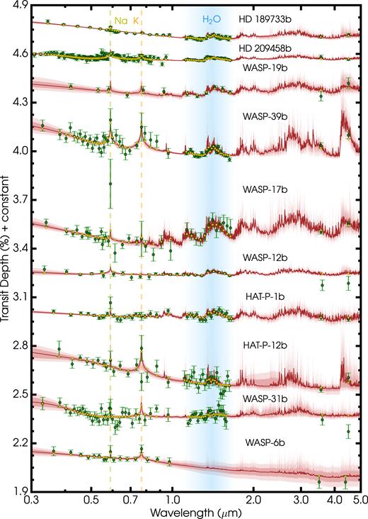
Retrieved model transmission spectra compared to observations for the ensemble of hot Jupiters. The data are shown in green and the retrieved median model is in dark red with associated 1σ and 2σ confidence contours. The yellow diamonds are the binned median model at the same resolution as the observations. The best-fitting median model in dark red has been smoothed for clarity. The data are discussed in Section 2 and shown in Table 1.
Prior information used in the retrieval analyses.
| Parameter | Prior | Prior range |
|---|---|---|
| Distribution | ||
| T0 | Uniform | 400 − Teq + 200 K (for |
| – | Teq < 1200 K) | |
| – | 800 − Teq + 200 K (for | |
| – | Teq > 1200 K) | |
| α1, 2 | Uniform | 0.02 − 1 K−1/2 |
| P1, 2 | Log-uniform | 10−6 − 102 bar |
| P3 | Log-uniform | 10−2 − 102 bar |
| Xi | Log-uniform | 10−12 − 10−2 |
| a | Log-uniform | 10−4 − 108 |
| γ | Uniform | -20 − 2 |
| Pcloud | Log-uniform | 10−6 − 102 bar |
| |$\bar{\phi }$| | Uniform | 0 − 1 |
Our results are presented as follows. In Section 4.1.1, we first discuss the most constrained parameter given the data: the H2O abundance. We then briefly consider other chemical species and their abundances in Section 4.1.2. We explore potential trends among the planetary parameters, H2O abundances, and cloud/haze properties in Section 4.2. We emphasize that the availability of optical HST STIS data for all planets allows a robust determination of H2O abundances, significantly reducing the degeneracies that arise from consideration of HST WFC3 data alone. This is exhibited in Section 4.3.
4.1 Chemistry
4.1.1 H2O Abundance
The H2O abundances are shown against planetary equilibrium temperature in Fig. 2. The reference ‘solar’ H2O indicates the H2O abundance as a function of temperature expected in hot Jupiter atmospheres with solar elemental abundances at a pressure of 1 bar (Asplund et al. 2009; Madhusudhan 2012). This is shown by the gold line in Fig. 2. For the majority of hot Jupiters considered in this work (i.e. those with equilibrium temperatures above ∼1300 K), H2O is expected to contain ∼50 per cent of the total available oxygen (Madhusudhan 2012) such that the solar water abundance is a constant and is |$X^{\odot} _{\mathrm{H_2O}} = \frac{1}{2} \frac{\rm O}{\rm H_{2}} \big|_{\odot}X^{\odot} _{\mathrm{H_2}}$|, where |$\frac{\rm O}{\rm H_2}|_{\odot} = 2 \frac{\rm O}{\rm H}|_{\odot}$| and log(|$X^{\odot }_{\mathrm{H_2O}}$|) = −3.3.
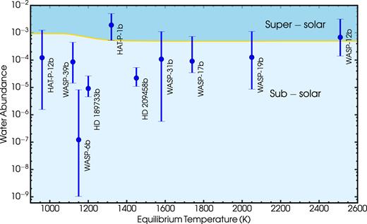
The retrieved H2O volume mixing ratios and their associated 1σ ranges for the hot Jupiter sample. The planets are consistent with subsolar H2O abundances within 1σ, excepting HAT-P-1b. The gold line shows the volume mixing ratio of water vapour calculated from solar elemental abundances (Madhusudhan 2012) and ranges from ∼10−3 at T ≲ 1200 K to 5 × 10⁻⁴ at higher temperatures.
The planets with the most precise observations in the HST WFC3 G141 bandpass – HD 189733b, HD 209458b, and WASP-12b – have retrieved |$\mathrm{log(X_{\mathrm{H_2O}})}$| abundances of |$-5.04^{+0.46}_{-0.30}$|, |$-4.66^{+0.39}_{-0.30}$|, and |$-3.16^{+0.66}_{-0.69}$|, respectively. The two hot Jupiters with the highest quality observations (HD 189733b and HD 209458b) show the most statistically significant H2O depletion and are consistent with those of previous studies (Madhusudhan et al. 2014a; Barstow et al. 2017; MacDonald & Madhusudhan 2017a). The inferred H2O abundance of WASP-12b is consistent to 1σ with that of another study (Kreidberg et al. 2015). HAT-P-1b, WASP-31b, WASP-17b, WASP-19b, and WASP-12b contain relative abundances of |$3.58^{+5.84}_{-2.60}\times$|, |$0.218^{+2.01}_{-0.217}\times$|, |$0.19^{+1.32}_{-0.12}\times$|, |$0.26^{+2.03}_{-0.24}\times$|, |$1.40^{+4.97}_{-1.11}\times$| solar which are consistent with subsolar and supersolar concentrations to within 1σ. The retrieved water abundances for the planets with the lowest equilibrium temperatures, HAT-P-12b and WASP-39b, are |$-3.91^{+1.01}_{-1.89}$| and |$-4.07^{+0.72}_{-0.78}$|, corresponding to |$0.133^{+1.226}_{-0.131}\times$| and |$0.10^{+0.42}_{-0.08}\times$| the solar abundance. The estimated water abundance for WASP-39b is inconsistent with that of another study (Wakeford et al. 2018) which used different WFC3 data than in this work. WASP-6b has the lowest derived abundance, consistent with a non-detection, owing largely to the lack of a HST WFC3 spectrum.
The H2O abundances, the solar-relative abundances, and the detection significances of water vapour are listed in Table 3. Considering the H2O abundance estimates for all the planets as an ensemble, the representative mixing ratio is log(X|$_{\mathrm{H_2O}}$|) = |$-4.20^{+0.20}_{-0.17}$| or about |$0.07^{+0.04}_{-0.02}\times$| solar. This ensemble value is inconsistent with a solar or supersolar abundance at 5.37σ assuming the objects come from the same population. Importantly, we have tested for effects of stellar heterogeneity using the CPAT model (Pinhas et al. 2018) and find no significant changes in the water abundances. We find no clear quantitative correlation between the H2O abundance and Teq.
Terminator H2O abundances, solar-normalized H2O abundances, and detection significances. The normalized H2O abundances are relative to the solar values shown by the gold line in Fig. 2. Detection significances are given for Bayes factors greater than 2.64 (i.e. 2σ).
| Planet | Log(|${X_{\mathrm{H_2O}}}_{-1\sigma }^{+1\sigma }$|) | Normalized abundance (|$X^{\odot }_{\mathrm{H_2O}})_{-1\sigma }^{+1\sigma }$| | Detection significance |
|---|---|---|---|
| HAT-P-12b | |$-3.91^{+1.01}_{-1.89}$| | |$0.133^{+1.226}_{-0.131}$| | N/A |
| WASP-39b | |$-4.07^{+0.72}_{-0.78}$| | |$0.10^{+0.42}_{-0.08}$| | 7.00σ |
| WASP-6b | |$-6.91^{+1.83}_{-2.07}$| | |$0.000156^{+0.014}_{-0.000155}$| | N/A |
| HD 189733b | |$-5.04^{+0.46}_{-0.30}$| | |$0.018^{+0.035}_{-0.009}$| | 5.60σ |
| HAT-P-1b | |$-2.72^{+0.42}_{-0.56}$| | |$3.58^{+5.84}_{-2.60}$| | 3.50σ |
| HD 209458b | |$-4.66^{+0.39}_{-0.30}$| | |$0.04^{+0.06}_{-0.02}$| | 7.06σ |
| WASP-31b | |$-3.97^{+1.01}_{-2.27}$| | |$0.218^{+2.01}_{-0.217}$| | 2.05σ |
| WASP-17b | |$-4.04^{+0.91}_{-0.42}$| | |$0.19^{+1.32}_{-0.12}$| | 3.22σ |
| WASP-19b | |$-3.90^{+0.95}_{-1.16}$| | |$0.26^{+2.03}_{-0.24}$| | 2.89σ |
| WASP-12b | |$-3.16^{+0.66}_{-0.69}$| | |$1.40^{+4.99}_{-1.11}$| | 5.73σ |
4.1.2 Other chemistry
We also constrain the presence and abundance of alkali absorbers in addition to H2O. Table 4 shows these elements which show clear modes in the retrieved posterior distributions with significances above 2σ. HD 189733b shows a confident detection of Na corresponding to a significance of 5.01σ (Bayes factor of 4.7 × 10⁴) and a subsolar value of |$-7.77^{+1.64}_{-0.87}$|. We detect potassium in WASP-6b at 2.67σ confidence with a constrained abundance of |$-5.53^{+2.01}_{-1.85}$|, consistent with the solar value. While there is a clear potassium signature in the spectrum of WASP-31b, the fidelity of this data point has recently been called into question (Gibson et al. 2017) and therefore WASP-31b is not included in Table 4. The retrieved posteriors for WASP-39b show evidence for CH4 and CO2 and yet may be due to a possible systematic offset between the HST and Spitzer data. Evidence of nitrogen-bearing molecules in these planetary atmospheres is examined in MacDonald & Madhusudhan (2017b).
Retrieved atomic species with detection significances above 2σ.
| Planet | Species | Detection significance | Abundance |
|---|---|---|---|
| WASP-39b | Na | 3.41σ | |$-3.86^{+1.31}_{-1.36}$| |
| K | 3.62σ | |$-4.22^{+1.25}_{-1.12}$| | |
| WASP-6b | K | 2.67σ | |${-5.53}^{+2.01}_{-1.85}$| |
| HD 189733b | Na | 5.01σ | |${-7.77}^{+1.64}_{-0.87}$| |
| HAT-P-1b | Na | 2.22σ | |$-8.44^{+1.45}_{-2.12}$| |
4.2 Exploring trends with planetary parameters, H2O abundances, and cloud/haze properties
We have carried out an extensive exploration of potential trends among planetary parameters, H2O abundances, and cloud/haze properties. We have investigated 35 combinations of pairs and triplets over the parameters Teq, Mp, g, |$X_{\mathrm{H_2O}}$|, |$\bar{\phi }$|, and Pcloud, resulting in no clear correlations. However, we present three parameter spaces and compare with analogous presentations in the literature (Sing et al. 2016; Stevenson 2016; Barstow et al. 2017). An extensive comparison with the methodologies and results of Sing et al. (2016) and Barstow et al. (2017) is presented in Section 5.
The terminator cloud/haze fractions (|$\bar{\phi }$|) versus H2O abundances with Teq as a third dimension are shown in Fig. 3. We do not find a clear trend between |$\bar{\phi }$| and H2O, and the cloud fractions for the planetary sample do not follow the clear-to-cloudy/hazy trend suggested by the spectral survey (Sing et al. 2016). The median cloud/haze fractions for WASP-12b and WASP-6b imply fewer aerosols and those for HD 209458b, WASP-31b, and HAT-P-12b imply more aerosols compared to a previously suggested order (Sing et al. 2016). Moreover, the derived grey cloud-top pressures (Pcloud) versus Teq are shown in Fig. 4. HD 189733b and WASP-6b likely have clouds composed of large particles deep in the atmospheres below ∼10−1 bar. On the other hand, opaque clouds with maximal cloud-top pressures of 0.1 mbar are found for HAT-P-12b, WASP-39b, HAT-P-1b, WASP-17b, WASP-19b, and WASP-12b but are relatively unconstrained. HD 209458b and WASP-31b have precise constraints of ∼0.5 dex on the cloud-top pressures and the cloud-tops lie above 1 mbar. Overall, we find no correlation between Teq and Pcloud. However, planets with low cloud-top pressures (below ∼1 mbar) span equilibrium temperatures of 1400–1600 K.
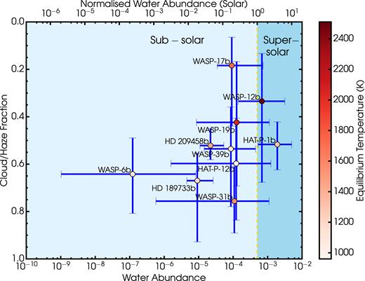
Terminator cloud/haze fractions, H2O abundances, and equilibrium temperatures of the hot Jupiter sample. The dashed gold line represents the solar water abundance at high temperatures (i.e. 5 × 10⁻⁴).
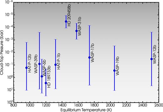
Top pressure of grey clouds versus planetary equilibrium temperature for the hot Jupiter ensemble.
Finally, the space of Teq, g, and |$\bar{\phi }$| is shown in Fig. 5. The lack of a clear correlation among these parameters is unlike previously suggested (Stevenson 2016). For the equilibrium temperatures spanned in our work (Teq > 700 K), Stevenson (2016) suggested that planets with log(g[cms−2]) greater than 2.8 are cloud-free whilst those below 2.8 should host a significant cloud fraction. In contrast, we find no such division, similar to a conclusion from a recent study (Barstow et al. 2017) of the spectral survey (Sing et al. 2016). This difference exists for at least two reasons. First, some of the G141 observations used in Stevenson (2016) are different than those we retrieve. Secondly, Stevenson (2016) explains the H2O feature amplitude with reference to clouds alone, assuming no variations over the H2O abundance. This assumption is too restrictive since a low-amplitude feature can imply peculiarly low water abundance with minimal cloud coverage and/or high Pcloud or a high water abundance with a significant cloud fraction and/or low Pcloud. On the other hand, the relatively clearer atmospheres of WASP-12b, WASP-19b, and WASP-17b shown in Fig. 5 support suggestions of hotter (|$T_{\mathrm{eq}} \gtrsim 1700\, \mathrm{K}$|) close-in planets harbouring less cloudy atmospheres (Liang et al. 2004; Heng 2016; Tsiaras et al. 2018).
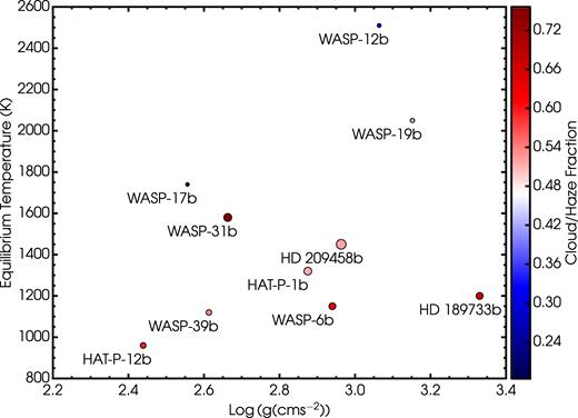
Cloud fractions |$\bar{\phi }$| as a function of Teq and planetary gravity. The marker size is inversely proportional with the retrieved 1σ confidence on the cloud fraction, such that finer constraints are represented with larger circles.
4.2.1 Metallicity and formation conditions
The retrieved set of H2O abundances provide initial clues on metal abundances in the exoplanetary atmospheres. Fig. 6 shows the space of atmospheric metallicity versus planet mass for the hot Jupiter sample in addition to previously reported metallicities of WASP-43b (Kreidberg et al. 2014), HAT-P-26b (Wakeford et al. 2017), and the solar system gas giants. The atmospheric metallicities are estimated from molecular species with well-determined abundances since knowledge of the full inventory of metals is limited by observational capabilities. The atmospheric metallicities for the hot Jupiter sample are calculated assuming that half of the oxygen is in the estimated H2O and the remaining half is in CO, in accordance with expectations for a solar C/O ratio in chemical equilibrium at high temperatures (Madhusudhan 2012). The atmospheric metallicities of the four solar system gas giants are determined from the abundance of methane which contains most of the carbon at their low temperatures (Atreya et al. 2016). The abundance of oxygen in the atmospheres of solar system planets cannot be incorporated into a metallicity estimate since much of it is condensed in deep-lying water clouds.
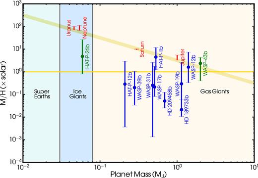
Atmospheric metal abundances as a function of planetary mass for the hot Jupiter ensemble. The planets in this study are shown in blue, along with WASP-43b (Kreidberg et al. 2014) and HAT-P-26b (Wakeford et al. 2017) from previous studies shown in green. The solar system giant planets are shown in red. The solar metallicity reference is shown by the horizontal gold line. WASP-6b is excluded due to lack of WFC3 observations. The exoplanetary atmosphere metallicities M/H of the giant exoplanets in our sample are derived from the H2O volume mixing ratio, such that M represents O, and assuming that half of the oxygen is in H2O as expected for a solar C/O ratio at high temperatures (Madhusudhan 2012). The metallicities of solar system planets are derived from the CH4 abundances, such that M represents C.
We emphasize that there are limitations to the illustration in Fig. 6 due to the different molecules used to represent the metallicities as well as using one molecular species as a metallicity descriptor. In principle, a high C/O ratio (e.g. C/O∼1) can lead to significantly subsolar H2O. Therefore, the low H2O abundances would indicate a low metallicity and/or a high C/O ratio (Madhusudhan et al. 2014a). The metallicity proxy for solar system planets shows a decreasing trend with increasing planetary mass. The subsolar hot Jupiter metallicities suggest a weak trend that is different from that of the solar system gas giants.
The inferred oxygen abundances provide initial clues into the formation and migration scenarios of these hot Jupiters when considering the metallicities of their host stars. The host stars of the majority of these hot Jupiters have O/H abundances in excess of the solar value (Teske et al. 2014; Brewer, Fischer & Madhusudhan 2017). This implies that the O/H ratios in the majority of the planetary atmospheres are substellar as well as being subsolar. Hot Jupiter atmospheres are expected to possess superstellar oxygen abundances if they are formed through core-accretion followed by migration within the disc (Madhusudhan et al. 2014b; Mordasini et al. 2016), as also suggested for Jupiter based on its supersolar abundances in several elements (Owen et al. 1999; Atreya & Wong 2005; Mousis et al. 2012).
On the other hand, the generally subsolar and substellar oxygen abundances found in these atmospheric spectra suggest a general scenario in which the hot Jupiters form far from their stars with efficient gas accretion and relatively inefficient solid planetesimal accretion (Madhusudhan et al. 2014a, 2016) since the gaseous O/H abundance is low in outer regions of protoplanetary discs due to successive condensation fronts of O-rich species (Öberg et al. 2011). Subsequent impulse inwards through gravitational interactions with other bodies in the system by disc-free migration may have brought many of these hot Jupiters to their present locations (Rasio & Ford 1996). Such disc-free migration could lead to low oxygen abundances irrespective of formation mechanisms, either core-accretion or gravitational instability (Madhusudhan et al. 2014b). Alternatively, some of the hot Jupiters may have formed through pebble accretion and migrated inward with or without the disc but without significant erosion of the core (Booth et al. 2017; Madhusudhan et al. 2017). The suggested importance of disc-free migration implied from the general trend of low oxygen abundances is consistent with proposals in other studies of the prevalence of disc-free migration based on dynamical properties of hot Jupiters and their environments (e.g. Brucalassi et al. 2016; Nelson, Ford & Rasio 2017).
4.3 Importance of optical data
The inclusion of optical data is essential in the interpretation of the hot Jupiter spectra, especially in the estimation of H2O abundances. The interpretation of HST WFC3 data alone introduces a well-known ambiguity between the reference pressure Pref and the water abundance |$X_{\mathrm{H_2O}}$| (e.g. see Griffith 2014). The use of HST STIS data to infer a reliable constraint on the reference pressure and the water abundance is illustrated in Fig. 7. In the retrieval of HST WFC3 data alone the line of ambiguity between Pref and |$X_{\mathrm{H_2O}}$| spreads over two orders of magnitude and the inferred |$X_{\mathrm{H_2O}}$| are mostly contained above 10−4. The same degeneracy disappears when optical HST STIS data are included in the retrieval; the joint posterior between Pref and |$X_{\mathrm{H_2O}}$| shows a well-localized set of solutions with no correlative trend. Moreover, the |$X_{\mathrm{H_2O}}$| values are constrained three times better and are contained below 10−4. The juxtaposition in Fig. 7 illustrates, in no unclear terms, that the broad ambiguity between Pref and |$X_{\mathrm{H_2O}}$| that exists for near-infrared WFC3 data alone collapses through the use of optical data, in this case HST STIS observations.
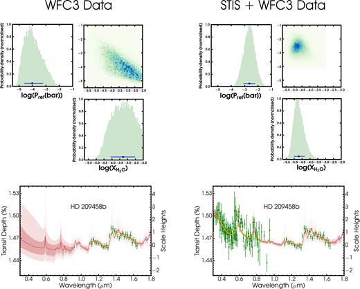
Demonstration of the use of optical data to precisely determine Pref and |$X_{\mathrm{H_2O}}$|. HD 209458b is used for illustration. One retrieval (left-hand column) inverts the HST WFC3 data and another retrieval (right-hand column) includes HST STIS data in the optical in addition to WFC3 data. The juxtaposition demonstrates that data in the optical range break the degeneracy between Pref and |$X_{\mathrm{H_2O}}$|.
5 DISCUSSION AND CONCLUSIONS
Here we compare our work with two previous studies: the spectral survey of Sing et al. (2016) that first reported the observations and Barstow et al. (2017) that conducted initial retrievals on those data sets. The differences between our work and these previous studies lie in both the modelling and retrieval approaches, as well as the results. At the outset, the key aspect of this work is the ability to derive statistical constraints (i.e. estimates with non-Gaussian error bars), along with full posterior distributions, for all the atmospheric parameters concerned. This allows one to pursue comparative exoplanetology for a sizeable exoplanet sample.
The differences in H2O abundances and cloud/haze properties between our findings and those of Sing et al. (2016) can be attributed to several crucial factors. First, the conclusions of the latter study were reached through a comparison of the data with equilibrium models of hot Jupiter atmospheres computed over a pre-determined grid in metallicity and temperature, as opposed to a full retrieval as in this study. Given the limited number of models in the grid and the equilibrium assumption, it was not possible to explore the model space adequately nor could the atmospheric properties be estimated statistically. This meant that it was necessary to invoke empirical metrics to qualitatively assess the contributions of the H2O abundance and clouds/hazes in the atmospheres. For example, the amplitude of the H2O feature at ∼1.4 μm was suggested to correlate with the difference between the planetary radius in the optical and infrared (Sing et al. 2016). However, this correlation was based on cloudy/hazy models which assumed solar and supersolar H2O abundances, without an exploration of cloudy/hazy atmospheres with subsolar water abundances as well as subsolar cloudy/hazy opacities (see their Fig. 3). As such, their conclusions were unable to reflect the full range of possible solutions, as confirmed in a follow-up study by Barstow et al. (2017) (discussed below) which found predominantly subsolar H2O solutions. Our study instead uses a comprehensive retrieval of all the data sets using a Bayesian nested sampling approach, enabling a detailed exploration of the entire multidimensional space of atmospheric parameters. We thereby assume no a priori values for the H2O abundances and cloud/haze properties.
There are also several differences between our study and that of Barstow et al. (2017). The differences are of three kinds: model parametrizations, statistical sampling algorithms, and reported estimates. We here discuss each of these in turn.
There are several important differences in the model parametrizations. The main aspect of the Barstow et al. (2017) study is that it is effectively a grid-based retrieval, in the sense that a separate retrieval is conducted for each assumption of a cloud prescription. Importantly, the study treats two kinds of cloud models separately: a model with Rayleigh-like slopes (i.e. our hazes) and one with grey opacity (i.e. our clouds). On the other hand, our cloud/haze model simultaneously accounts for small and large particle sizes (see equation 4). An important distinction also lies in the aerosol parametrization. Our study includes a grey cloud overlain by a haze such that both types of aerosols are retrieved for a planet, although the retrieved parameters could indicate no hazes (i.e. a = 1 and γ = −4) and/or no grey clouds (i.e. Pcloud ≳ 10 bar). On the other hand, Barstow et al. (2017) allows for the presence of a vertically finite cloud or haze deck at variable locations in the atmosphere. In some cases (e.g. HD 189733b) where our study retrieves a deep cloud layer with an extensive overlying haze layer, Barstow et al. (2017) retrieve a decade-confined haze layer confined to low pressures. These two different interpretations, however, produce similar fits to the spectrum.
An additional crucial difference in the aerosol models is that this study accounts for inhomogeneous clouds and hazes along the planetary limb. The inclusion of patchy clouds is important since the shape of the H2O feature in the WFC3 bandpass is sensitive to the degree of cloud contribution (e.g. see Line & Parmentier 2016). These differences in modelling are likely another principal element responsible for discrepancies in the cloud and haze properties between this work and that of Barstow et al. (2017). Secondly, Barstow et al. (2017) assumes an isotherm for the observable region of the atmosphere (pressures below 0.1 bar) whereas we allow a fully general temperature profile that allows for any temperature gradient. Thirdly, there is a significant difference in the treatment of opacity in the radiative transfer. Whereas the previous study assumes the correlated-k distribution for opacities, our study uses opacity sampling from very high-resolution cross-sections for the different molecules. This difference in opacity treatments could potentially influence the retrievals. However, generally similar water abundance estimates between the two methods is encouraging. Fourthly, the cloud properties and temperature profiles in Barstow et al. (2017) were pre-defined on a grid, whereas the atmospheric parameters in our study are sampled continuously over the entire parameter space.
There are also important differences in the statistical inference methods. Barstow et al. (2017) uses an optimal estimation (OE) sampler whereas our analysis uses a Bayesian nested sampling algorithm, MultiNest. First, while OE has been shown to be accurate for very high-resolution data, its accuracy has been shown to be limited for low-resolution spectrophotometry (Line et al. 2013), as is relevant in the present case. On the other hand, the MultiNest Bayesian analysis approach has been shown to be more accurate for the quality of hot Jupiter data considered here since it is able to explore parameter spaces with multimodal solutions (Feroz & Hobson 2008; Feroz et al. 2013). Secondly, the OE sampler in Barstow et al. (2017) requires assuming Gaussian-distributed uncertainties in the model parameters whereas no such assumption is required in the present Bayesian approach. This is significant since the derived parameter posteriors in our study indeed show mostly non-Gaussian distributions. Thirdly, given the efficiency of our modelling and retrieval approach a much larger volume of the high-dimensional model parameter space is explored for each planet (i.e. ∼5 × 10⁶ models) while the approach in Barstow et al. (2017) was limited to 3,600 model evaluations per planet.
Finally, there are important differences regarding the nature of reported parameter estimates. First, Barstow et al. (2017) does not provide statistical estimates on the abundances and other atmospheric properties but instead provide parameter values of a select set of model fits to the data. On the other hand, our analysis provides statistical limits, along with full posteriors, for all the atmospheric parameters through consideration of all model evaluations. Hence, our estimated median values and 1σ uncertainties are obtained through marginalization over the full posteriors. Secondly, the cloud/haze properties and temperatures profiles in Barstow et al. (2017) were pre-defined on a grid and hence joint constraints on these properties and chemistry are not possible. Our approach allows for complete marginalization over all parameters and hence provides joint statistical correlations between all atmospheric parameters, thereby enabling a more extensive illumination of the atmospheres.
The considerations above naturally lead to differences between our results and those of the Barstow et al. (2017) study, particularly on the nature of clouds. Barstow et al. (2017) finds three planets – WASP-39b, HD 209458b, and WASP-31b – are best fit by grey opacity clouds with top pressures of 10−5, 0.01, and 0.1 bar, respectively. Fig. 4 shows the retrieved cloud-top pressures for HD 209458b and WASP-31b are smaller by ∼2 dex and that of WASP-39b is larger by ∼4 dex. A comparison with other planets in the sample is not possible since the cloud-top pressures in the previous study are quoted for pure Rayleigh clouds (Barstow et al. 2017), that is, only for clouds composed of small particles.
In addition, a trend is suggested in the analysis of Barstow et al. (2017) such that planets with equilibrium temperatures spanning 1,300 to 1,700K possess grey clouds that are confined deep in their atmospheres below ∼10 mbar (Barstow et al. 2017). On the other hand, our analysis finds that HAT-P-1b (Teq = 1320 K), HD 209458b (Teq = 1450 K), and WASP-31b (Teq = 1580 K) are consistent with high-altitude grey cloud-top pressures (see Fig. 4). WASP-17b and WASP-12b, with equilibrium temperatures above 1700 K, have also been suggested to have good evidence for small-particle aerosols at high atmospheric altitudes (Barstow et al. 2017). We find that a model without hazes or clouds composed of small particles provides statistically comparable fits to the spectra of WASP-17b and WASP-12b, and is suggestive of weak evidence for small-particle aerosols in their atmospheres.
The discussion above illustrates that there are differences in the retrieved cloud properties between our analysis and that of Barstow et al. (2017) which may be attributed to the different approaches of cloud/haze modelling. In spite of these differences, we emphasize that the estimated water abundances in the hot Jupiter atmospheres are generally in good agreement and show a trend towards subsolar values. Planets for which similar WFC3 data are used (HD 189733b, HD 209458b, WASP-31b, WASP-17b, and WASP-19b) illustrate that the H2O abundances can be robust to different aerosol treatments in retrieval studies.
Beyond the key advancements in the modelling approach, the Bayesian inference method, and the results, the major contribution of our work is to provide detailed statistical estimates of important atmospheric properties for a sizable sample of hot Jupiters. All in all, these estimates will prove invaluable for comparative planetology, across both exoplanetary and solar system giant planets and for understanding their formation pathways.
In summary, we have carried out a comprehensive atmospheric study of transmission observations of a sizeable giant exoplanet sample contained in Sing et al. (2016). Through a homogeneous Bayesian retrieval analysis of the planetary spectra, we determine statistically robust estimates of various atmospheric parameters including the H2O abundances, cloud/haze properties, other chemical abundances, and temperature profiles. In particular, we find that all the planetary atmospheres are consistent in harbouring subsolar H2O abundances within 1σ with the exception of HAT-P-1b. The planets with the most precise observations in the HST WFC3 G141 bandpass – HD 189733b, HD 209458b, and WASP-12b – are constrained to have H2O abundances of |$0.018^{+0.035}_{-0.009}\times$|, |$0.04^{+0.06}_{-0.02}\times$|, and |$1.40^{+4.97}_{-1.11}\times$| solar, respectively. We find a continuum over cloud and haze contributions as suggested in recent studies (Sing et al. 2016; Barstow et al. 2017), although the details are different than suggested therein.
The lack of a clear correlation among various properties of the atmospheres and macroscopic properties of the planets is consistent with a unique and detailed evolutionary history for each giant exoplanet. Nevertheless, in light of the host stars’ solar or supersolar O/H metallicities and the generally subsolar O/H abundances, the majority of close-in hot giant exoplanets are suggested to form beyond the H2O ice-line with subsequent dynamical interaction and disc-free migration to their present environments.
ACKNOWLEDGEMENTS
AP is grateful for research support from the Gates Cambridge Trust. NM, SG, and RM acknowledge support from the Science and Technology Facilities Council (STFC), UK. We thank the reviewer for useful comments that have helped improve the manuscript. This research has made use of the SVO Filter Profile Service supported from the Spanish MINECO through grant AyA2014-55216. We thank the contributors of the Python Software Foundation, the Open Science Framework, and NASA’s Astrophysics Data System.
Footnotes
REFERENCES
APPENDIX A: COMPLETE RETRIEVED PARAMETERS
Retrieved chemical abundances of the hot Jupiter sample.
| Planet | Mp (MJ) | XNa† | XK† | |$X_{\mathrm{H_2O}}$|† | |$X_{\mathrm{CH_4}}$|† | |$X_{\mathrm{NH_3}}$|† | XHCN† | XCO† | |$X_{\mathrm{CO_2}}$|† |
|---|---|---|---|---|---|---|---|---|---|
| HAT-P-12b | |$0.21^{+0.01}_{-0.01}$| | |${-8.75}^{+2.92}_{-2.16}$| | |${-3.24}^{+0.89}_{-4.25}$| | |$\mathbf { {-3.91}^{+1.01}_{-1.89}}$| | |${-9.14}^{+2.00}_{-1.82}$| | |${-8.98}^{+2.10}_{-1.94}$| | |${-8.43}^{+2.64}_{-2.28}$| | |${-5.65}^{+2.77}_{-4.02}$| | |${-6.16}^{+2.21}_{-3.39}$| |
| WASP-39b | |$0.28^{+0.03}_{-0.03}$| | |${-3.86}^{+1.31}_{-1.36}$| | |${-4.22}^{+1.25}_{-1.12}$| | |$\mathbf { {-4.07}^{+0.72}_{-0.78}}$| | |${-5.65}^{+0.78}_{-1.02}$| | |${-8.65}^{+2.28}_{-2.16}$| | |${-8.24}^{+2.53}_{-2.43}$| | |${-7.02}^{+3.08}_{-3.22}$| | |${-4.31}^{+0.91}_{-1.04}$| |
| WASP-6b | |$0.50^{+0.02}_{-0.04}$| | |${-9.18}^{+2.14}_{-1.82}$| | |${-5.53}^{+2.01}_{-1.85}$| | |$\mathbf { {-6.91}^{+1.83}_{-2.07}}$| | |${-9.15}^{+1.97}_{-1.83}$| | |${-8.62}^{+2.20}_{-2.17}$| | |${-8.60}^{+2.25}_{-2.18}$| | |${-7.77}^{+2.93}_{-2.69}$| | |${-10.08}^{+1.76}_{-1.29}$| |
| HD 189733b | |$1.14^{+0.03}_{-0.03}$| | |${-7.77}^{+1.64}_{-0.87}$| | |${-8.87}^{+1.38}_{-1.52}$| | |$\mathbf { {-5.04}^{+0.46}_{-0.30}}$| | |${-9.18}^{+1.86}_{-1.84}$| | |${-9.09}^{+1.99}_{-1.91}$| | |${-8.13}^{+2.38}_{-2.55}$| | |${-6.93}^{+2.97}_{-3.33}$| | |${-9.02}^{+1.84}_{-1.96}$| |
| HAT-P-1b | |$0.53^{+0.02}_{-0.02}$| | |${-8.44}^{+1.45}_{-2.12}$| | |${-9.10}^{+1.92}_{-1.84}$| | |$\mathbf { {-2.72}^{+0.42}_{-0.56}}$| | |${-8.39}^{+2.37}_{-2.29}$| | |${-7.85}^{+2.66}_{-2.64}$| | |${-7.65}^{+2.78}_{-2.79}$| | |${-7.29}^{+3.15}_{-3.05}$| | |${-8.93}^{+2.11}_{-1.96}$| |
| HD 209458b | |$0.69^{+0.02}_{-0.02}$| | |${-4.92}^{+0.83}_{-0.57}$| | |${-6.46}^{+0.84}_{-0.64}$| | |$\mathbf { {-4.66}^{+0.39}_{-0.30}}$| | |${-8.60}^{+2.20}_{-2.22}$| | |${-8.56}^{+2.22}_{-2.28}$| | |${-8.66}^{+2.25}_{-2.21}$| | |${-8.37}^{+2.57}_{-2.38}$| | |${-9.80}^{+1.57}_{-1.45}$| |
| WASP-31b | |$0.48^{+0.03}_{-0.03}$| | |${-7.66}^{+2.76}_{-2.68}$| | |${-3.43}^{+0.95}_{-1.62}$| | |$\mathbf { {-3.97}^{+1.01}_{-2.27}}$| | |${-8.30}^{+2.42}_{-2.34}$| | |${-5.01}^{+1.52}_{-4.45}$| | |${-7.92}^{+2.64}_{-2.59}$| | |${-7.32}^{+3.15}_{-3.01}$| | |${-9.20}^{+2.09}_{-1.83}$| |
| WASP-17b | |$0.49^{+0.03}_{-0.03}$| | |${-8.71}^{+1.55}_{-1.76}$| | |${-9.77}^{+1.55}_{-1.38}$| | |$\mathbf { {-4.04}^{+0.91}_{-0.42}}$| | |${-9.26}^{+1.76}_{-1.73}$| | |${-8.33}^{+2.34}_{-2.32}$| | |${-8.70}^{+2.25}_{-2.10}$| | |${-5.41}^{+2.46}_{-4.13}$| | |${-7.04}^{+1.86}_{-2.77}$| |
| WASP-19b | |$1.11^{+0.04}_{-0.04}$| | |${-7.51}^{+2.75}_{-2.80}$| | |${-7.10}^{+2.48}_{-2.63}$| | |$\mathbf { {-3.90}^{+0.95}_{-1.16}}$| | |${-8.76}^{+2.16}_{-2.05}$| | |${-8.44}^{+2.40}_{-2.23}$| | |${-8.03}^{+2.71}_{-2.48}$| | |${-6.45}^{+3.04}_{-3.48}$| | |${-7.03}^{+2.28}_{-2.97}$| |
| WASP-12b | |$1.40^{+0.10}_{-0.10}$| | |${-4.11}^{+1.30}_{-1.75}$| | |${-8.88}^{+2.29}_{-2.00}$| | |$\mathbf { {-3.16}^{+0.66}_{-0.69}}$| | |${-8.84}^{+2.09}_{-1.99}$| | |${-8.47}^{+2.28}_{-2.19}$| | |${-8.17}^{+2.47}_{-2.41}$| | |${-7.18}^{+3.10}_{-3.00}$| | |${-8.34}^{+2.43}_{-2.32}$| |
Note: †All values are in log10(Xi).
| Planet | Mp (MJ) | log10(a) | γ | log10(Pcloud) | |$\bar{\phi }$| |
|---|---|---|---|---|---|
| HAT-P-12b | |$0.21^{+0.01}_{-0.01}$| | |${4.70}^{+1.66}_{-1.74}$| | |${-9.04}^{+4.62}_{-7.78}$| | |${-0.78}^{+1.80}_{-2.03}$| | |${0.60}^{+0.24}_{-0.19}$| |
| WASP-39b | |$0.28^{+0.03}_{-0.03}$| | |${3.83}^{+1.22}_{-1.10}$| | |${-13.27}^{+4.29}_{-4.24}$| | |${-1.09}^{+2.01}_{-2.53}$| | |${0.54}^{+0.24}_{-0.18}$| |
| WASP-6b | |$0.50^{+0.02}_{-0.04}$| | |${4.92}^{+2.04}_{-1.41}$| | |${-6.06}^{+1.99}_{-2.63}$| | |${-0.10}^{+1.34}_{-1.38}$| | |${0.64}^{+0.17}_{0.15}$| |
| HD 189733b | |$1.14^{+0.03}_{-0.03}$| | |${3.64}^{+0.79}_{-1.01}$| | |${-7.75}^{+1.29}_{-1.43}$| | |${0.44}^{+1.03}_{-1.13}$| | |${0.67}^{+0.26}_{-0.12}$| |
| HAT-P-1b | |$0.53^{+0.02}_{-0.02}$| | |${5.68}^{+1.52}_{-1.49}$| | |${-5.77}^{+2.49}_{-3.09}$| | |${-1.02}^{+1.93}_{-2.03}$| | |${0.52}^{+0.11}_{-0.10}$| |
| HD 209458b | |$0.69^{+0.02}_{-0.02}$| | |${4.57}^{+0.58}_{-0.74}$| | |${-14.82}^{+4.79}_{-3.45}$| | |${-4.47}^{+0.52}_{-0.48}$| | |${0.52}^{+0.06}_{-0.07}$| |
| WASP-31b | |$0.48^{+0.03}_{-0.03}$| | |${4.00}^{+0.95}_{-0.98}$| | |${-14.08}^{+4.07}_{-3.69}$| | |${-3.72}^{+0.66}_{-0.61}$| | |${0.76}^{+0.13}_{-0.15}$| |
| WASP-17b | |$0.49^{+0.03}_{-0.03}$| | |${2.33}^{+2.20}_{-2.53}$| | |${-10.55}^{+5.66}_{-5.84}$| | |${-1.60}^{+2.21}_{-2.56}$| | |${0.18}^{+0.26}_{-0.12}$| |
| WASP-19b | |$1.11^{+0.04}_{-0.04}$| | |${3.95}^{+2.00}_{-2.22}$| | |${-11.52}^{+5.29}_{-5.11}$| | |${-0.56}^{+1.60}_{-1.97}$| | |${0.42}^{+0.27}_{-0.26}$| |
| WASP-12b | |$1.40^{+0.10}_{-0.10}$| | |${2.07}^{+2.64}_{-2.87}$| | |${-10.47}^{+7.11}_{-6.47}$| | |${-1.48}^{+2.14}_{-2.15}$| | |${0.33}^{+0.34}_{-0.20}$| |
Retrieved temperature profile parameters of the hot Jupiter sample.
| Planet | T0 | α1 | α2 | P1† | P2† | P3† | Pref† |
|---|---|---|---|---|---|---|---|
| HAT-P-12b | |${456}^{+70}_{-40}$| | |${0.81}^{+0.13}_{-0.17}$| | |${0.63}^{+0.24}_{-0.28}$| | |${-1.54}^{+1.63}_{-1.74}$| | |${-3.97}^{+1.74}_{-1.34}$| | |${0.61}^{+0.94}_{-1.32}$| | |${-2.68}^{+0.84}_{-0.40}$| |
| WASP-39b | |${775}^{282}_{-166}$| | |${0.66}^{+0.22}_{-0.21}$| | |${0.59}^{+0.27}_{-0.26}$| | |${-1.50}^{+1.64}_{-1.77}$| | |${-3.99}^{+1.92}_{-1.35}$| | |${0.60}^{+0.95}_{-1.37}$| | |${-2.55}^{+0.52}_{-0.39}$| |
| WASP-6b | |${1057}^{+198}_{-290}$| | |${0.57}^{+0.26}_{-0.22}$| | |${0.60}^{+0.26}_{-0.25}$| | |${-1.70}^{+1.61}_{-1.65}$| | |${-4.06}^{+1.79}_{-1.30}$| | |${0.49}^{+1.00}_{-1.33}$| | |${-3.55}^{+0.60}_{-0.74}$| |
| HD 189733b | |${1159}^{+146}_{-157}$| | |${0.76}^{+0.16}_{-0.22}$| | |${0.67}^{+0.22}_{-0.27}$| | |${-1.70}^{+1.75}_{-1.83}$| | |${-3.98}^{+1.85}_{-1.35}$| | |${0.48}^{+1.05}_{-1.42}$| | |${-2.07}^{+0.23}_{-0.43}$| |
| HAT-P-1b | |${1114}^{+251}_{-205}$| | |${0.65}^{+0.22}_{-0.22}$| | |${0.59}^{+0.26}_{-0.25}$| | |${-1.58}^{+1.61}_{-1.72}$| | |${-4.04}^{+1.83}_{-1.31}$| | |${0.57}^{+0.95}_{-1.30}$| | |${-3.63}^{+0.42}_{-0.41}$| |
| HD 209458b | |${949}^{+252}_{-109}$| | |${0.59}^{+0.27}_{-0.20}$| | |${0.35}^{+0.38}_{-0.17}$| | |${-1.85}^{+1.66}_{-1.28}$| | |${-4.22}^{+1.80}_{-1.22}$| | |${0.05}^{+1.29}_{-1.07}$| | |${-2.65}^{+0.39}_{-0.43}$| |
| WASP-31b | |${1043}^{+287}_{-172}$| | |${0.69}^{+0.21}_{-0.23}$| | |${0.61}^{+0.25}_{-0.26}$| | |${-1.64}^{+1.65}_{-1.75}$| | |${-4.04}^{+1.84}_{-1.32}$| | |${0.54}^{+0.98}_{-1.37}$| | |${-3.43}^{+0.61}_{-0.53}$| |
| WASP-17b | |${1147}^{+259}_{-305}$| | |${0.58}^{+0.26}_{-0.21}$| | |${0.58}^{+0.26}_{-0.24}$| | |${-1.52}^{+1.51}_{-1.68}$| | |${-3.99}^{+1.82}_{-1.33}$| | |${0.55}^{+0.95}_{-1.26}$| | |${-2.38}^{+0.32}_{-0.66}$| |
| WASP-19b | |${1386}^{+370}_{-337}$| | |${0.66}^{+0.22}_{-0.22}$| | |${0.61}^{+0.24}_{-0.24}$| | |${-1.69}^{+1.64}_{-1.66}$| | |${-3.99}^{+1.74}_{-1.33}$| | |${0.49}^{+0.98}_{-1.33}$| | |${-2.83}^{+0.89}_{-0.76}$| |
| WASP-12b | |${990}^{+169}_{-122}$| | |${0.77}^{+0.15}_{-0.18}$| | |${0.66}^{+0.22}_{-0.26}$| | |${-1.55}^{+1.65}_{-1.71}$| | |${-3.92}^{+1.79}_{-1.35}$| | |${0.60}^{+0.93}_{-1.38}$| | |${0.16}^{+0.64}_{-0.63}$| |
Note: †All values are in log10(Pi[bar]).
