A novel 3D technique to study the kinematics of lensed galaxies

Rizzo, Francesca; Vegetti, Simona; Fraternali, Filippo; Di Teodoro, Enrico

doi:10.1093/mnras/sty2594

Abstract

We present a 3D Bayesian method to model the kinematics of strongly lensed galaxies from spatially resolved emission-line observations. This technique enables us to simultaneously recover the lens–mass distribution and the source kinematics directly from the 3D data cube. We have tested this new method with simulated OSIRIS observations for nine star-forming lensed galaxies with different kinematic properties. The simulated rotation curves span a range of shapes that are prototypes of different morphological galaxy types, from dwarf to massive spiral galaxies. We have found that the median relative accuracy on the inferred lens and kinematic parameters are at the level of 1 and 2 per cent, respectively. We have also tested the robustness of the technique against different inclination angles, signal-to-noise ratios, the presence of warps, or non-circular motions and we have found that the accuracy stays within a few per cent in most cases. This technique represents a significant step forward with respect to the methods used until now, as the lens parameters and the kinematics of the source are derived from the same 3D data. This enables us to study the possible degeneracies between the two and estimate the uncertainties on all model parameters consistently.

gravitational lensing: strong, methods: data analysis, galaxies: high-redshift, galaxies: kinematics and dynamics

1 INTRODUCTION

Measuring the content of baryons and dark matter within galaxies, and its evolution with redshift, is a key test of galaxy formation models. In the context of ΛCDM cosmology, current numerical simulations have not yet produced consistent predictions on the fraction of dark matter within young galaxies. In particular, the amount of dark matter fraction within the stellar half-mass radius has been shown to be strongly dependent on the implementation of feedback processes (e.g. Wu et al. 2014; Remus et al. 2017; Teklu et al. 2018). For example, different simulations (e.g. Lovell et al. 2018; Teklu et al. 2018) have resulted in dark matter fraction at |$z$| ∼ 2 that can differ by almost one order of magnitude. Numerous physical mechanisms, such as the mass accretion history, the initial mass function, dynamical instabilities, and adiabatic contraction, determine the relative contribution of baryons and dark matter within a galaxy (e.g. Blumenthal et al. 1986; Dutton et al. 2011; Courteau & Dutton 2015; Zolotov et al. 2015). For this reason, quantifying the amount of dark matter from kinematical measurements provides a strong constraint on galaxy formation models (Rubin, Ford & Thonnard 1978; van Albada et al. 1985).

From an observational perspective, a number of observations have revealed that a significant number of high-redshift galaxies are a disc-dominated system (e.g. Förster Schreiber et al. 2006, 2009; Wisnioski et al. 2015; Mason et al. 2017). However, while in the Local Universe the flatness of the rotation curves and the matter content of disc galaxies is a well-established fact, at high redshift it is currently a matter of debate, with rotation curves having flat (Di Teodoro, Fraternali & Miller 2016), rising (Tiley et al. 2016), or declining shapes (Genzel et al. 2017; Lang et al. 2017). The declining rotation curves for six star-forming galaxies at redshift between 0.8 and 2.3 have been explained, for example, by Lang et al. (2017) and Genzel et al. (2017) as an indication of baryon-dominated systems, with a fraction of dark matter lower than 0.2. On the other hand, Di Teodoro et al. (2016), Di Teodoro et al. (2018), and Mason et al. (2017) have derived rotation curves and velocity dispersion values in agreement with those of local star-forming galaxies (Epinat et al. 2010).

The partition of the matter content between dark matter, stars, and gas within a galaxy is provided, also, by studying the evolution of the stellar mass Tully–Fisher relation (TFR; Tully & Fisher 1977), which correlates the stellar mass to the rotation velocity, a tracer of the total dynamical mass. A change in the normalization with redshift might, for example, indicate a redistribution of the total mass between visible and dark matter.

Even if the TFR has been explored at redshifts between 0 and 4 by numerous studies, there is no consensus whether it evolves (e.g. Puech et al. 2008; Straatman et al. 2017; Turner et al. 2017; Übler et al. 2017) or not (e.g. Miller et al. 2011, 2012; Di Teodoro et al. 2016; Harrison et al. 2017) with redshift.

The diverging results on the kinematics of high-redshift galaxies and, as a consequence of their matter content, can be ascribed to the different methods used to overcome the observational limitations. The study of the kinematics is mainly hampered by two factors: low spatial resolutions and low signal-to-noise ratios (SNRs). Seeing-limited observations are typically characterized by an effective spatial resolution of 5 kpc at the redshifts of the sources, |$z$| ∼ 1–2 (e.g. Förster Schreiber et al. 2009; Swinbank et al. 2017), while a handful of adaptive optic (AO) observations have achieved higher resolutions of ∼1–1.6 kpc (Molina et al. 2017; Förster Schreiber et al. 2018). Furthermore, because of cosmological surface-brightness dimming, only the bright central regions of galaxies can be observed, especially with AO. Although AO observations are characterized by a better spatial resolution with respect to seeing-limited observations, they have a worse sensitivity and a data binning is often required to increase the SNR.

One of the consequences of limited spatial resolution is to smooth out the measured rotation velocity via the so-called beam-smearing effect and can result in an overestimation of the velocity dispersion (e.g. Wright et al. 2009; Newman et al. 2013; Di Teodoro & Fraternali 2015). This effect can also lead to a misclassification of objects: for example, Newman et al. (2013) have shown that the fraction of dispersion-dominated galaxies in the SINS/zC-SINF surveys (Cresci et al. 2009; Förster Schreiber et al. 2009; Genzel et al. 2011) drops from 41 per cent at a seeing-limited resolution to 6–9 per cent when galaxies are observed in the AO mode.

The observational limitations imposed by low resolution and SNR can be successfully overcome by targeting strongly gravitationally lensed galaxies. Strong gravitational lensing offers the opportunity to study high-redshift galaxies at a much higher physical resolution and SNR in their source plane (e.g. Nesvadba et al. 2006; Swinbank et al. 2007). Furthermore, the magnifying power of gravitational lensing opens the possibility to study galaxies in the low-stellar-mass range of 5 × 10⁸–|$5\times 10^9 \, \mathrm{M}_\odot$| (e.g. Jones et al. 2010a; Leethochawalit et al. 2016; Mason et al. 2017), which is instead not easily achievable by surveys targeting unlensed galaxies (e.g. Förster Schreiber et al. 2006; Swinbank et al. 2012a).

It was only in recent years that the potential of gravitational lensing has started to be exploited: for example, Stark et al. (2008) have studied the kinematics of a lensed galaxy at a resolution of 120 pc at |$z$| = 3.07. The analysis of two larger samples then followed this study: Jones et al. (2010a) have analysed six lensed galaxies in the redshift range 1.7–3.1, and Livermore et al. (2015) have further extended this sample to 17 targets with redshift from 1 to 4. Leethochawalit et al. (2016) have analysed 15 lensed galaxies at |$z$| ∼ 2. Regarding the galaxy population properties, Jones et al. (2010a) and Leethochawalit et al. (2016) have used different methods to distinguish well-ordered velocity fields from disturbed/merging kinematics and obtained a different classification for similar ranges of redshift and stellar mass: 36 per cent of the galaxies in the Leethochawalit et al. (2016) sample are rotationally dominated and as many as 66 per cent in the Jones et al. (2010a) sample, as confirmed by Livermore et al. (2015).

So far, most of the analysis aimed at studying the kinematics of lensed sources with optical emission lines has been characterized by the following features:

the lens–mass model is derived from high-spatial-resolution-imaging data (e.g. from HST images; Stark et al. 2008; Jones et al. 2010b, 2013; Shirazi et al. 2014; Livermore et al. 2015; Leethochawalit et al. 2016; Yuan et al. 2017);
the kinematic modelling is done either by delensing the 3D Integral Field Unit (IFU) data (e.g. Jones et al. 2013; Livermore et al. 2015) and deriving the velocity and dispersion maps with a Gaussian fit to the emission lines in the source plane, or by deriving the moment maps in the image plane and then delensing these maps to the source plane (e.g. Jones et al. 2010b; Leethochawalit et al. 2016). In both cases, the lens model is kept fixed.
A functional form, usually an arctangent function, is used to fit the delensed velocity field and derive the rotation curve.

Recent studies based on molecular line observations have used a similar approach (e.g. Dye et al. 2015; Rybak et al. 2015b; Swinbank et al. 2015). One first derives the lens–mass distribution from the radio continuum, observed in the same bands as the molecular lines. Then, this model is used to derive the 3D-line data and calculate the corresponding moment maps in the source plane. Finally, kinematic parameters are derived either by applying the kinemetry method (Krajnović et al. 2006) to both the first- and second-moment maps (Rybak et al. 2015b) or by applying a dynamical model to the first-moment map (Dye et al. 2015; Swinbank et al. 2015).

All these approaches are suboptimal mainly for two reasons: first, if the lens model is kept fixed, it is not possible to quantify any degeneracy between the lens–mass parameters and the source kinematic properties. Secondly, the kinematic fitting is done on the reconstructed source rather than on the data. However, on the source plane, pixels are correlated, the noise properties not fully characterized, and the effective resolution changes with position according to the lensing magnification. As a consequence, one introduces systematic errors in the derivation of the kinematic properties of the source, which may be difficult to quantify.

Recently, Patrício et al. (2018) have applied a forward modelling approach that partly overcomes some of the above issues by deriving the velocity map directly on the image plane through a Gaussian fitting to the emission lines. However, similarly to the techniques described above, this method is not ideal, as it relies on a fixed lens model derived from a separate HST observation and it performs a kinematic modelling of the 2D velocity map, instead of the full 3D data cube.

Finally, other studies have been focusing on sources that are not significantly lensed (i.e. only weakly distorted), so that the kinematic analysis can be done directly on the image plane without having to reconstruct the unlensed emission (e.g. Mason et al. 2017; Di Teodoro et al. 2018; Girard et al. 2018). However, even small distortions of the observed axis ratio, due to lensing, could affect the capability to recover the kinematic parameters accurately. Mason et al. (2017) have tried to correct for this effect using a global value for the magnification factor.

In this paper, we present a novel Bayesian three-dimensional and pixellated approach, which, applied either to IFU or interferometric data, enables us to simultaneously reconstruct both the lensing mass distribution and the kinematics of the source. Our method represents a significant improvement over those described above as it is not affected by differential magnification nor poor understanding of the errors and resolution properties of the reconstructed unlensed plane. Our technique does not require the use of high-resolution imaging data for the derivation of the lens parameters, as these are derived from the same 3D data used for the modelling of the kinematics of the background galaxy. Since the lens parameters and the source are inferred simultaneously from the same data set, our method is not affected by differential magnification. Moreover, the kinematics of the background galaxy is not obtained by fitting on the source plane, but directly the lensed data in a hierarchical Bayesian fashion, where the kinematics on the source plane is essentially a hyper-parameter (i.e. parameter defining the prior) of the model. The main novelty of our procedure is that a modified tilted-ring kinematic model is an extra constraint for a pixellated source reconstruction. Furthermore, the derivation of the lens–mass model and the source kinematics is done simultaneously, allowing us to quantify possible degeneracies and to estimate the errors on all model parameters using a Bayesian approach. Finally, our 3D approach enables us to describe the kinematics of the source minimizing the influence of the beam-smearing effect.

This paper is organized as follows. In Section 2, we describe in detail the method used for the lens modelling and the derivation of the kinematics. In Section 3, we present the IFU-simulated data sets. In Section 4, we describe the modelling strategy and the assumptions applied to model the simulated data sets, which are then used in Section 5 to test our method under different observational set-ups. The robustness and the limits of the technique are summarized in Section 6, where we also list future developments and applications.

2 METHOD DESCRIPTION

This section describes the core features of our method, which is an extension of the technique developed by Vegetti & Koopmans (2009) to the 3D-domain. In particular, we present the statistical framework that allows us to reconstruct the background source, its kinematics, and the lens–mass distribution. The lens–mass parametrization is described in Section 2.2, while the details of the kinematic model used to describe the lensed source are given in Section 2.3.

2.1 Source reconstruction

In the following, we indicate with |$\mathbf {{\boldsymbol{s}}}$| and |$\mathbf {{\boldsymbol{d}}}$| the 3D pixellated surface brightness distribution of the source and the data in the image plane, respectively. We refer the reader to Fig. 1 for a schematic representation of the source and image planes.

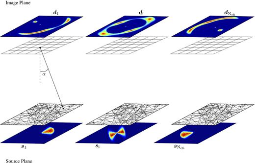
$A schematic view of the source and lens planes. On the upper panel, the lensed data for three representative spectral channels and the respective regular grid on the image plane. For each spectral channel, the position $\vec{x}$ of a subset of $\mathrm{\text{$N$}_{s}}$ pixels in the image plane corresponds to a position $\vec{y}$ on the source plane (lower panel), through the lens equation $\vec{y}=\vec{x}-\vec{\alpha }\left(\vec{x}\right)$. The points $\vec{y}$ are the vertices of a triangular adaptive grid on the source plane.$

Figure 1.

A schematic view of the source and lens planes. On the upper panel, the lensed data for three representative spectral channels and the respective regular grid on the image plane. For each spectral channel, the position |$\vec{x}$| of a subset of |$\mathrm{\text{$N$}_{s}}$| pixels in the image plane corresponds to a position |$\vec{y}$| on the source plane (lower panel), through the lens equation |$\vec{y}=\vec{x}-\vec{\alpha }\left(\vec{x}\right)$|⁠. The points |$\vec{y}$| are the vertices of a triangular adaptive grid on the source plane.

Open in new tab Download slide

Given a set of |$\mathrm{N_{ch}}$| observed spectral channels, the source and data vectors, |${{\boldsymbol{s}}}$| and |${{\boldsymbol {d}}}$|⁠, have a total of |$\mathrm{N_{ch}}$| components, |$\boldsymbol {s}_{\mathrm{i}..\mathrm{N_{ch}}}$| and |$\boldsymbol {d}_{\mathrm{i}..\mathrm{N_{ch}}}$|⁠, respectively, each representing the surface brightness distribution in one channel i:

\begin{eqnarray*} \mathbf {{\boldsymbol{s}}}=\lbrace \boldsymbol {s}_{1}, ..., \boldsymbol {s}_{\mathrm{i}}, ..., \boldsymbol {s}_\mathrm{N_{ch}}\rbrace, \end{eqnarray*}

(1)

\begin{eqnarray*} \mathbf {{\boldsymbol{d}}}=\lbrace \boldsymbol {d}_{1}, ..., \boldsymbol {d}_{\mathrm{i}}, ..., \boldsymbol {d}_{\mathrm{N_{ch}}}\rbrace. \end{eqnarray*}

(2)

For each ith spectral channel, the surface brightness distribution of the lensed cube |$\boldsymbol {d}_{\mathrm{i}}$|⁠, its noise |$\boldsymbol {n}_{\mathrm{i}}$|⁠, and the relative unknown source surface brightness distribution |$\boldsymbol {s}_{\mathrm{i}}$| are related to each other by the following set of linear equations:

\begin{eqnarray*} {\boldsymbol{\sf M}}\left(\boldsymbol{\psi }\right)\boldsymbol {s}_{\mathrm{i}}+ \boldsymbol {n}_{\mathrm{i}}=\boldsymbol {d}_{\mathrm{i}}, \end{eqnarray*}

(3)

where |$\rm {\boldsymbol{\sf M=B\, L}}$| is the response operator that depends on the lensing operator |${\boldsymbol{\sf L}}$| and the point spread function (PSF) operator |${\boldsymbol{\sf B}}$| (for interferometric data, |${\boldsymbol{\sf B}}$| is the Fourier transfer operator). The lensing operator |${\boldsymbol{\sf L}}$| is a non-linear function of the lens mass–density distribution parameters |$\boldsymbol{\eta _{\mathrm{lens}}}$| (see Section 2.2 for their definition) via the lensing potential |$\psi \left(\boldsymbol{\eta _{\mathrm{lens}}}\right)$|⁠.

The method used for the source reconstruction is grid-based in the sense that the background–source surface brightness distribution is reconstructed on a triangular adaptive grid defined by a Delaunay tessellation. The source grid automatically adapts with the lensing magnification, so that there is a high pixel-density in the high-magnification regions close to the caustics. The vertices of the triangular grid are obtained by casting back to the source plane a subset |$\mathrm{N_{s}}$| of the |$\mathrm{N_{d}}$| image–plane pixels via the lens equation. We determine the surface brightness at each source-plane pixel by interpolating between the values at the vertices of the triangles. We reconstruct each channel on the same triangulation.

As both |$\boldsymbol{\eta _{\mathrm{lens}}}$| and the source |$\boldsymbol {s}_{\mathrm{i}}$| are unknown, equation (3) is ill-defined and cannot be simply inverted. Therefore, we derive a penalty function defined in the context of three levels of Bayesian inference, which are described below.

2.1.1 First level of inference – linear optimization

Using Bayes’ rule, the most probable a posteriori source, |$\mathbf {\text{$\boldsymbol{s}$}_{\rm MP}}$|⁠, given the data and a lens–mass model, is derived by maximizing the following posterior probability (Suyu et al. 2006; Vegetti & Koopmans 2009):

\begin{eqnarray*} P\left(\mathbf {{\boldsymbol{s}}}|\mathbf {{\boldsymbol{d}}}, \lambda , \boldsymbol{\eta _{\mathrm{lens}}}, \boldsymbol{\eta _{\mathrm{kin}}},{\boldsymbol{\sf R}}\right)=\frac{P\left(\mathbf {{\boldsymbol{d}}}|\mathbf {{\boldsymbol{s}}}, \boldsymbol{\eta _{\mathrm{lens}}}\right) P\left(\mathbf {{\boldsymbol{s}}} | \lambda , \boldsymbol{\eta _{\mathrm{kin}}}, {\boldsymbol{\sf R}}\right)}{P \left(\mathbf {{\boldsymbol{d}}}| \lambda , \boldsymbol{\eta _{\mathrm{lens}}}, \boldsymbol{\eta _{\mathrm{kin}}}, {\boldsymbol{\sf R}}\right)}. \end{eqnarray*}

(4)

Here, the matrix |${\boldsymbol{\sf R}}$| is the source regularization form (variance, gradient, or curvature), with a strength set by the regularization level vector λ (see Koopmans 2005; Vegetti & Koopmans 2009, for further details). The regularization level vector λ has |$\mathrm{\text{$N$}_{ch}}$| components, so that the user can choose whether the level of regularization is constant across the spectral channels or not. For simplicity, all equations below and above assume a constant value of λ as a function of frequency. |$\boldsymbol{\eta _{\mathrm{kin}}}$| in equation (4) are the source kinematic parameters, as defined in Section 2.3. The remaining terms in equation (4) are the likelihood function |$P\left(\mathbf {{\boldsymbol{d}}}|\mathbf {{\boldsymbol{s}}}, \boldsymbol{\eta _{\mathrm{lens}}}\right)$|⁠, the prior on the source surface brightness distribution |$P\left(\mathbf {{\boldsymbol{s}}} | \lambda , \boldsymbol{\eta _{\mathrm{kin}}}, \mathbf {R}\right)$|⁠, and the evidence |$P\left(\mathbf {{\boldsymbol{d}}}| \lambda , \boldsymbol{\eta _{\mathrm{lens}}},\boldsymbol{\eta _{\mathrm{kin}}}, {\boldsymbol{\sf R}}\right)$|⁠, which is irrelevant for the maximization of the posterior, but plays an important role at the third level of inference (see Section 2.4). Under the assumption of Gaussian noise, the likelihood can be expressed as follows:

\begin{eqnarray*} P\left(\mathbf {{\boldsymbol{d}}}|\mathbf {{\boldsymbol{s}}}, \boldsymbol{\eta _{\mathrm{lens}}}\right)=\frac{\exp \left[-E_{\mathrm{D}}\left(\mathbf {{\boldsymbol{d}}}|\mathbf {{\boldsymbol{s}}}, \boldsymbol{\eta _{\mathrm{lens}}}\right)\right]}{Z_{\mathrm{D}}}, \end{eqnarray*}

(5)

where Z_D is the normalization, and E_D is half the standard χ² and is given by

\begin{eqnarray*} E_{\mathrm{D}}\left(\mathbf {{\boldsymbol{d}}}|\mathbf {{\boldsymbol{s}}}, \boldsymbol{\eta _{\mathrm{lens}}}\right)=\frac{1}{2} \sum _{\mathrm{\text{$i$}}=1}^{\mathrm{N_{ch}}}\left({\boldsymbol{\sf M}}\boldsymbol {s}_{\mathrm{i}}-\boldsymbol {d}_{\mathrm{i}}\right)^{\intercal }{\boldsymbol{\sf C}}_{\mathrm{d\, i}}^{-1}\left({\boldsymbol{\sf M}}\boldsymbol {s}_{\mathrm{i}}-\boldsymbol {d}_{\mathrm{i}}\right). \end{eqnarray*}

(6)

Above, |${\boldsymbol{\sf C}}_{\mathrm{d\, i}}$| is the covariance matrix of the data for the ith spectral channel. Since the noise is assumed to be uncorrelated, it is a diagonal matrix.

In our implementation, the source prior assumes a quadratic form, which peaks at a source kinematic model, |$\mathbf {\text{$\boldsymbol{s}$}_{\mathrm{kin}}\left(\boldsymbol{\eta _{\mathrm{kin}}}\right)}$|⁠. The prior probability distribution is, therefore, expressed as

\begin{eqnarray*} P\left(\mathbf {{\boldsymbol{s}}} | \lambda , \boldsymbol{\eta _{\mathrm{kin}}}, {\boldsymbol{\sf R}}\right)=\frac{\exp \left[-\lambda E_{\mathrm{R}}\left(\mathbf {{\boldsymbol{s}}}|\boldsymbol{\eta _{\mathrm{kin}}}, {\boldsymbol{\sf R}}\right)\right]}{Z_{\mathrm{R}}}, \end{eqnarray*}

(7)

where the quadratic functional E_R and the normalization Z_R are given, respectively, by

\begin{eqnarray*} E_{\mathrm{R}}\left(\mathbf {{\boldsymbol{s}}}\right)= \sum _{\mathrm{i}=1}^{\mathrm{N_{ch}}} \left[E_{\mathrm{R}}\left(\boldsymbol {s}_{\mathrm{kin\, i}}\right)+\frac{1}{2}\left(\boldsymbol {s}_{\mathrm{i}}-\boldsymbol {s}_{\mathrm{kin\, i}}\right)^{\intercal } {\boldsymbol{\sf H}}_{\mathrm{R, i}}\left(\boldsymbol {s}_{\mathrm{i}}-\boldsymbol {s}_{\mathrm{kin\, i}}\right)\right] \end{eqnarray*}

(8)

and

\begin{eqnarray*} Z_{\mathrm{R}}\left(\lambda \right)=\int \text{d}^{\mathrm{N_{s}}}\mathbf {{\boldsymbol{s}}}\, e^{-E_{\mathrm{R}}\left(\mathbf {s}\right)}=e^{-E_{\mathrm{R}}\left(\mathbf {s_{kin}}\right)}\left(\frac{2\pi }{\lambda } \right)^{\frac{\mathrm{N_{s}N_{ch}}}{2}}\left(\det {\boldsymbol{\sf H}}_{\mathrm{R}}\right)^{-\mathrm{N_{ch}/2}}. \nonumber \\ \end{eqnarray*}

(9)

|${\boldsymbol{\sf H}}_{\mathrm{R}}$| in the above equation is a block matrix made up of the N_ch matrices |${\boldsymbol{\sf H}}_{\mathrm{R, i}}$| (see equation (8)) and it is defined as the Hessian of E_R, |${\boldsymbol{\sf H}}_{\mathrm{R}}=\nabla \nabla E_{\mathrm{R}}={\boldsymbol{\sf R}}^{\intercal }{\boldsymbol{\sf R}}$|⁠. The most probable surface brightness is obtained by maximizing the posterior probability in equation (4), i.e. by solving the following set of linear equations:

\begin{eqnarray*} \left[{\boldsymbol{\sf M}}^{\intercal }{\boldsymbol{\sf C}}_{\mathrm{d\, i}}^{-1}{\boldsymbol{\sf M}}+\lambda {\boldsymbol{\sf H}}_{\mathrm{R}}\right]\boldsymbol {s}_{i}={\boldsymbol{\sf M}}^{\intercal }{\boldsymbol{\sf C}}_{\mathrm{d\, i}}^{-1}\boldsymbol {d}_{\mathrm{i}}+\lambda {\boldsymbol{\sf H}}_{\mathrm{R}}\boldsymbol {s}_{\mathrm{kin\, i}}. \end{eqnarray*}

(10)

The form of these equations differs from those derived in Vegetti & Koopmans (2009) in the last term on the right-hand side, |$\lambda {\boldsymbol{\sf H}}_{\mathrm{R i}}\boldsymbol {s}_{\mathrm{kin\, i}}$|⁠. This term is due to a different assumption about the peak of the source prior, which is equal to zero in Vegetti & Koopmans (2009) and |$\mathbf {\text{$\boldsymbol{s}$}_{\mathrm{kin}}}$| here.

2.1.2 Second level of inference – non-linear optimization

To infer the kinematic parameters |$\boldsymbol{\eta _{\mathrm{kin}}}$|⁠, the lens parameters |$\boldsymbol{\eta _{\mathrm{lens}}}$|⁠, and the optimal level of regularization λ, we maximize the following posterior probability:

\begin{eqnarray*} P\left(\lambda , \boldsymbol{\eta _{\mathrm{kin}}}, \boldsymbol{\eta _{\mathrm{lens}}}|\mathbf {{\boldsymbol{d}}},{\boldsymbol{\sf R}}\right)=\frac{P\left(\mathbf {{\boldsymbol{d}}}|\lambda , \boldsymbol{\eta _{\mathrm{lens}}}, \boldsymbol{\eta _{\mathrm{kin}}}, {\boldsymbol{\sf R}}\right) P\left(\lambda , \boldsymbol{\eta _{\mathrm{kin}}}, \boldsymbol{\eta _{\mathrm{lens}}}\right)}{P\left(\mathbf {{\boldsymbol{d}}}|{\boldsymbol{\sf R}}\right)}. \nonumber \\ \end{eqnarray*}

(11)

Assuming a prior that is flat in logλ, |$\boldsymbol{\eta _{\mathrm{lens}}}$|⁠, and |$\boldsymbol{\eta _{\mathrm{kin}}}$|⁠, equation (11) can be expressed as

\begin{eqnarray*} P\left(\mathbf {{\boldsymbol{d}}}|\lambda , \boldsymbol{\eta _{\mathrm{lens}}},\boldsymbol{\eta _{\mathrm{kin}}}, \mathbf {R}\right)= \int \, P\left(\mathbf {{\boldsymbol{d}}}|\mathbf {{\boldsymbol{s}}}, \boldsymbol{\eta _{\mathrm{lens}}}\right)P\left(\mathbf {{\boldsymbol{s}}} | \lambda , \boldsymbol{\eta _{\mathrm{kin}}}, {\boldsymbol{\sf R}}\right)\, \text{d}\mathbf {{\boldsymbol{s}}}. \end{eqnarray*}

(12)

If we assume a Gaussian noise and a quadratic form of regularization, equation (12) can be written as

\begin{eqnarray*} &&{P\left(\mathbf {{\boldsymbol{d}}}|\lambda , \boldsymbol{\eta _{\mathrm{lens}}}, \boldsymbol{\eta _{\mathrm{kin}}}, \mathbf {R}\right) = -E\left(\mathbf {\text{$\boldsymbol{s}$}_{MP}}\right)-\frac{\mathrm{N_{ch}}}{2}\log {\det {\boldsymbol{\sf H}}_{\mathrm{E}}} +\frac{\mathrm{N_{s}N_{ch}}}{2}\log {\lambda }} \nonumber \\ &&{\quad + \lambda E_{\mathrm{s}}\left(\mathbf {\text{$\boldsymbol{s}$}_{kin}}\right)+\frac{\mathrm{N_{ch}}}{2}\log {\det {\boldsymbol{\sf H}}_{\mathrm{R}}}-\frac{\mathrm{N_{d}N_{ch}}}{2}\log {2\pi }-\frac{1}{2}\sum _{\mathrm{\text{$i$}}=1}^{\mathrm{N_{ch}}} \log {\det {\boldsymbol{\sf C}}_{\mathrm{d\, i}}}.} \nonumber \\ \end{eqnarray*}

(13)

In the above equation, E = E_D + λE_R, |${\boldsymbol{\sf H}}_{\mathrm{E}}$| is its Hessian, and |$\mathbf {\text{$\boldsymbol{s}$}_{MP}}$| is the most probable solution that maximizes the posterior, |$\nabla E \left(\mathbf {\text{$\boldsymbol{s}$}_{MP}}\right) = 0$|⁠.

The expression for the posterior probability, equation (13), differs from that derived by Suyu et al. (2006) and Vegetti & Koopmans (2009) for the multiplications/summation by/over |$\mathrm{\text{$N$}_{ch}}$| and the presence of the term |$E_{\mathrm{s}}\left(\mathbf {\text{$\boldsymbol{s}$}_{kin}}\right)$|⁠, which is the main novelty of our approach. This allows us to derive the kinematic parameters of the source, while retaining the flexibility of a pixellated source surface brightness distribution, simultaneously infer the lens-mass distribution, and take advantage of the extra constraints provided by the velocity channels.

2.1.3 Third level of inference – model comparison

At the third level of inference, to compare and rank different models, we calculate the marginalized Bayesian evidence that is a measure of the probability of the data given by the model. In our case, this marginalized evidence can be expressed as the integral of the normalization factor in equation (4) over the lens parameters |$\boldsymbol{\eta _{\mathrm{lens}}}$|⁠, the kinematic parameters |$\boldsymbol{\eta _{\mathrm{kin}}}$|⁠, and the source regularization λ, such that

\begin{eqnarray*} P\left(\mathbf {{\boldsymbol{d}}}|{\boldsymbol{\sf R}}\right) &=& \int P\left(\mathbf {{\boldsymbol{d}}}|\lambda , \boldsymbol{\eta _{\mathrm{lens}}}, \boldsymbol{\eta _{\mathrm{kin}}}, {\boldsymbol{\sf R}}\right) \nonumber \\ &&\times \, P\left(\lambda , \boldsymbol{\eta _{\mathrm{lens}}},\boldsymbol{\eta _{\mathrm{kin}}}\right)\, \text{d}\lambda \, \text{d}\boldsymbol{\eta _{\mathrm{lens}}}\, \text{d}\boldsymbol{\eta _{\mathrm{kin}}}. \end{eqnarray*}

(14)

This integral is calculated numerically with multinest (Feroz, Hobson & Bridges 2009; Feroz et al. 2013), which is a Nested Sampling-based method improving on the original idea by Skilling (2004). As a by-product of this evidence calculation, we also obtain the posterior distributions of the model parameters, allowing us to estimate their statistical uncertainties and degeneracies (see Section 5).

2.2 Lens–mass model

The lens parameters |$\boldsymbol{\eta _{\mathrm{lens}}}$| that define the lensing operator |${\boldsymbol{\sf L}}$| are as follows: κ₀, q, γ, x₀, y₀, θ, Γ_sh, θ_sh. These parameters describe a projected mass density profile as a cored elliptical power-law distribution with the contribution of an external shear component of strength Γ_sh and position angle θ_sh. The dimensionless projected mass density profile is defined as

\begin{eqnarray*} \kappa \left(x,y\right)=\frac{\kappa _0\left(2-\frac{\gamma }{2}\right)q^{\gamma -\frac{3}{2}}}{2\left[q^2\left(x^2+r_{\mathrm{c}}^2\right)+y^2\right]^{\frac{\gamma -1}{2}}}. \end{eqnarray*}

(15)

Here, κ₀ is the surface mass–density normalization, q is the projected flattening, γ is the density slope, x₀ and y₀ define the centre of the mass distribution, r_c is the core radius, and θ is the position angle of the major axis. The Einstein radius for this density profile is defined as

\begin{eqnarray*} R_{\mathrm{ein}}=\left[\frac{\kappa _0\left(2-\frac{\gamma }{2}\right)q^{\frac{\gamma -2}{2}}}{3-\gamma }\right]^{\frac{1}{\gamma -1}}. \end{eqnarray*}

(16)

In the following sections, we assume that the mass distribution has a negligible core radius of 10⁻⁴ arcsec.

2.3 Source kinematic model

We build the kinematic model using a modified version of the building-model function of ^3Dbarolo (Di Teodoro & Fraternali 2015). To simulate the gas emission from a rotating galaxy, the ^3Dbarolo algorithm uses a stochastic function that populates a 6D domain (three spatial and three spectral dimensions) with emitting gas clouds, which allow us to build the line profiles. The rotating galaxy is modelled as a series of concentric circular rings using the so-called tilted-ring model (Rogstad, Lockhart & Wright 1974). On each ring, the positions of the clouds are chosen randomly in such a way that, on average, the clouds become uniformly distributed over its surface. Each ring is described by the following parameters:

the coordinates of the centre x_s, y_s;
the inclination angle i, defined such that i = 90° for an edge-on galaxy and i = 0° for a face-on one;
the position angle PA, defined as the angle between the north direction of the sky and the projected major axis of the receding half of the rings measured counterclockwise;
the face-on gas column density Σ;
the systemic velocity V_sys;
the rotation velocity V_rot;
the velocity dispersion σ_gas.

The projected velocity along the line-of-sight V_los at a particular radius R is defined by

\begin{eqnarray*} V_{\mathrm{los}}\left(R\right)=V_{\mathrm{sys}} +V_{\mathrm{rot}}\left(R\right) \cos {\phi } \sin {i}, \end{eqnarray*}

(17)

where ϕ is the azimuthal angle in the plane of the galaxy. To build the 3D model, at each radius, the positions of the clouds are then rotated and projected into the plane of the sky with an orientation with respect to the observer defined by both the position and the inclination angles at that radius. As in ^3Dbarolo, to obtain the velocity profile at each location, the clouds are divided into subclouds. Each of these subclouds has a velocity which is drawn from a Gaussian distribution with a dispersion of |$\sigma ^2= \sigma ^2_{\mathrm{gas}}+\sigma ^2_{\mathrm{instr}}$|⁠. Here, σ_instr takes into account the instrumental broadening.

Unlike ^3Dbarolo , our implementation does not allow for a variation of all the parameters ring by ring. Instead, we make the following assumptions: (i) all the rings have the same centre coordinates and systemic velocity (in Section 5.10, we explicitly test the effects of this assumption); (ii) the radial variations of the inclination and position angles are described by a polynomial of deg from 0 to 3; (iii) the radial variations of the rotation velocity and velocity dispersion are described by functional forms. The use of functional forms for the rotation velocity and velocity dispersion allows us to reduce the number of free parameters. Our kinematic model |$\mathbf {\text{$\boldsymbol{s}$}_{\mathrm{kin}}}$| is, therefore, defined by the following set of parameters |$\boldsymbol{\eta _{\mathrm{kin}}}=\lbrace R_{\mathrm{ext}}, \Sigma , x_{\mathrm{s}}, y_{\mathrm{s}}, V_{\mathrm{sys}}, i, PA, V_{\mathrm{rot}}, \sigma _{\mathrm{gas}}\rbrace$|⁠. R_ext is the radial extension and is a fixed parameter chosen by the user. In Section 4, we describe the assumptions made to estimate R_ext for the simulated data analysed in this paper. Following ^3Dbarolo, the surface density of the gas Σ is also not a free parameter; instead, we impose a pixel-by-pixel normalization, which is given by the surface brightness distribution obtained from the lens modelling of the zeroth-moment map. The advantage of using a spatially changing normalization is that it allows us to take into account for possible asymmetries in the ionized or molecular gas distribution, as it is typical for high-redshift galaxies given the presence of massive star-forming regions (e.g. Genzel et al. 2011; Swinbank et al. 2012b; Livermore et al. 2015). Therefore, the presence of clumpy emissions or holes should not affect the derived kinematics, because this normalization ensures that the kinematics is independent of the gas distribution (e.g. Lelli et al. 2012; Di Teodoro & Fraternali 2015).

By construction, the kinematic model is built on a Cartesian grid, defined by a pixel scale and dimensions chosen by the user. Since the source reconstruction is determined on a Delaunay tessellation (see Section 2.1), we then map this model at the positions of the triangle vertices.

2.3.1 Rotation velocity and velocity dispersion curves

We have implemented three empirical functions to describe the rotation curves: the arctangent function (Courteau 1997), the hyperbolic tangent function (Andersen et al. 2001), and a multiparameter function (Rix et al. 1997). These are expressed by the following three expressions, respectively:

\begin{eqnarray*} V_{\mathrm{rot}}\left(R\right) = \frac{2}{\pi }\, V_{\mathrm{t}}\, \arctan \left(\frac{R}{R_{\mathrm{t}}}\right), \end{eqnarray*}

(18)

\begin{eqnarray*} V_{\mathrm{rot}}\left(R\right) = V_{\mathrm{t}}\, \tanh \left(\frac{R}{R_{\mathrm{t}}}\right), \end{eqnarray*}

(19)

\begin{eqnarray*} V_{\mathrm{rot}}\left(R\right) = V_{\mathrm{t}}\frac{\left(1+\frac{R_{\mathrm{t}}}{R}\right)^{\beta }}{\left[1+\left(\frac{R_{\mathrm{t}}}{R}\right)^{\xi }\right]^{1/\xi }}. \end{eqnarray*}

(20)

R_t is the turnover radius between the inner rising and outer part of the curve. V_t is the asymptotic velocity for the arctangent and hyperbolic tangent functions, and the velocity scale for the multiparameter one. ξ defines the sharpness of the turnover while β specifies the power-law behaviour of the curve at large radii. The arctangent function has mainly been used to model the kinematics of high-redshift galaxies (e.g. Swinbank et al. 2012a; Leethochawalit et al. 2016). However, it is not flexible enough to reproduce the different kinds of observed rotation curves, especially in the inner regions where a bump can be present. For this reason, we prefer the multiparameter function which is, by definition, more flexible.

To describe the velocity dispersion profile, the user can choose from a power-law, a linear, or an exponential function:

\begin{eqnarray*} \sigma _{\mathrm{gas}}\left(R\right) = \sigma _{0}\, \left(\frac{R}{R_{\sigma }}\right)^{\zeta }, \end{eqnarray*}

(21)

\begin{eqnarray*} \sigma _{\mathrm{gas}}\left(R\right) = \sigma _{0}+\zeta \, R, \end{eqnarray*}

(22)

\begin{eqnarray*} \sigma _{\mathrm{gas}}\left(R\right) = \sigma _{0}\, e^{-\frac{R}{R_{\sigma }}}+\sigma _{1}. \end{eqnarray*}

(23)

2.4 Optimization scheme

We infer the unknown parameters |$\boldsymbol{\eta _{\mathrm{lens}}}$|⁠, λ, |$\boldsymbol{\eta _{\mathrm{kin}}}$| and the source |$\mathbf {{\boldsymbol{s}}}$| with an optimization scheme, which is divided into the following four stages (see also Fig. 2 for a schematic view):

To find a good initial guess for the lens model parameters, |$\boldsymbol{\eta _{\mathrm{lens}}}$|⁠, we start by modelling the zeroth-moment map of the data. This optimization is performed in three separate substeps. First, λ is kept fixed at a relatively large value, such that the source model remains relatively smooth, and |$P\left(\boldsymbol{\eta _{\mathrm{lens}}}|\lambda , \mathbf {{\boldsymbol{d}}},{\boldsymbol{\sf R}}\right)$| is maximized relatively to |$\boldsymbol{\eta _{\mathrm{lens}}}$|⁠. Secondly, the lens parameters are kept fixed at the most probable values found at the previous step, while |$P\left(\lambda |\boldsymbol{\eta _{\mathrm{lens}}}, \mathbf {{\boldsymbol{d}}},{\boldsymbol{\sf R}}\right)$| is optimized for the source regularization level λ. Finally, |$P\left(\boldsymbol{\eta _{\mathrm{lens}}}|\lambda , \mathbf {{\boldsymbol{d}}},{\boldsymbol{\sf R}}\right)$| is maximized again for the lens parameters with a source regularization level fixed to the most probable value determined in the previous stage. At every point of the non-linear mass-model optimization, the corresponding most probable source surface brightness distribution |$\mathbf {\text{$\boldsymbol{s}$}_{\rm MP}}$| is obtained by solving the linear system (10) with |$\mathbf {\text{$\boldsymbol{s}$}_{kin}}=0$|⁠.
We now model the entire 3D data cube. Assuming the values of |$\boldsymbol{\eta _{\mathrm{lens}}}$| found in step (i), we infer the optimal regularization constant λ and |$\boldsymbol{\eta _{\mathrm{kin}}}$|⁠, maximizing equation (13) by varying first the kinematic parameters that define |$\mathbf {\text{$\boldsymbol{s}$}_{kin}}$|⁠, then the source regularization level λ, and finally the kinematic parameters again. At this stage, the user can choose between a value of the regularization level λ that is the same for all of the spectral channels or a value that varies channel by channel.
We repeat the process described in (i), using equations (11) and (10) with |$\boldsymbol{\eta _{\mathrm{kin}}}$| equal to the value found in (ii).
Finally, the lens parameters, λ, and only the kinematic parameters that describe the rotation velocity and velocity dispersion, i.e. V_rot, σ_gas, are simultaneously left free to vary, starting from the values of the parameters found at the previous steps. As for the last two, at this stage, we focus on the 3D data cube.

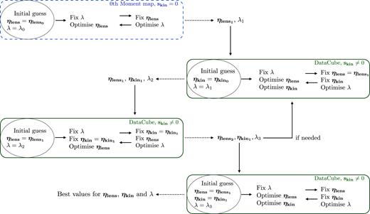
$A schematic overview of the four-step optimization scheme used to infer the unknown parameters $\boldsymbol{\eta _{\mathrm{lens}}}$, λ, $\boldsymbol{\eta _{\mathrm{kin}}}$. The four boxes represent the points (i)–(iv) in Section 2.4. An initial estimate of the lens parameters is obtained by fitting the zeroth-moment map, while for the successive steps the full 3D data cube is used.$

Figure 2.

A schematic overview of the four-step optimization scheme used to infer the unknown parameters |$\boldsymbol{\eta _{\mathrm{lens}}}$|⁠, λ, |$\boldsymbol{\eta _{\mathrm{kin}}}$|⁠. The four boxes represent the points (i)–(iv) in Section 2.4. An initial estimate of the lens parameters is obtained by fitting the zeroth-moment map, while for the successive steps the full 3D data cube is used.

Open in new tab Download slide

The analysis described at the points (ii) and (iii) is repeated if a visual inspection of the residuals reveals a mismatch between the model and the data. All of the optimization steps described above are done with a non-linear optimizer (i.e. a Downhill–Simplex with Simulated Annealing; Press et al. 1992). As discussed in Section 2.1.3, the calculation of the Bayesian evidence with multinest allows us to explore the parameter space and obtain the posterior distributions of the parameters. In this case, both the kinematic and lens parameters are simultaneously changed.

3 IFU MOCK DATA

To investigate the ability of our new modelling technique to recover reliable lens and kinematic parameters, we simulate nine observations of H α emission from star-forming lensed galaxies at redshifts between ∼1.3 and ∼2.4. In particular, we use the technical features of the OSIRISspectrograph (Larkin et al. 2006). We have chosen to focus on OSIRIS because it has the typical characteristics of a near-infrared integral field spectrometer mounted on an 8–10 m telescope in terms of spatial resolution, AO performances, and spectral resolution, with a typical channel width of 30–40 km s⁻¹.

To simulate the lensed data, we first build a cube from a rotating galaxy (Section 3.1), we then lens it forward using the lens–mass model described in Section 2.2. Finally, we convolve the lensed cube with a spatial PSF and add the noise (Section 3.2).

3.1 Simulated sources

The lensed sources have redshifts between 1.3 and 2.4 (column 2 in Table 1) which results in their Hα emission line falling in the H or K filters (column 4 in Table 1). The total H α fluxes (column 7 in Table 1) have values typical of star-forming galaxies at |$z$| ∼ 1–2 (e.g. Förster Schreiber et al. 2009; Livermore et al. 2015). The average resolving power is ∼3400 corresponding to |${\sim }6\,\,{\mathring{\rm A} }$| in these bands. The cube of the rotating galaxy is built using ^3Dbarolo(Di Teodoro & Fraternali 2015). Input values for the geometrical and kinematical parameters that define the inclination i and position angle PA and the rotation velocity V_rot and dispersion σ_gas are listed in Table 1. The sources have an extension of ∼5–8 kpc along the major axis, as typical of |$z$| ∼ 1–2 galaxies (e.g. Wisnioski et al. 2015; Leethochawalit et al. 2016; Genzel et al. 2017; Patrício et al. 2018).

Table 1.

Open in new tab

Observational and physical properties for the nine mock systems. Top table: Column 1: name of the data set. Column 2: redshift of the source. Column 3: redshift of the lens. Columns 4–5: OSIRIS filter and the corresponding FOV. Column 6: FWHM for the core + halo PSF (see Section 3.1). Middle table: Kinematic parameters used to create the source. Bottom table: Lens parameters used to lens the source and to create the observed mock data.

Observation set-up
Mock data set	\|$z$\|_source	\|$z$\|_lens	Filter	FOV	FWHM	FHα	t_exp
				arcsec	arcsec	10⁻¹⁸ erg s⁻¹ cm⁻²	ks
M1	2.05	0.881	Kn1	3.6 × 6.4	0.17 + 0.95	15	14.4
M2	2.19	0.191	Kn2	4.5 × 6.4	0.17 + 0.95	20	14.4
M3	2.15	0.722	Kn2	4.5 × 6.4	0.17 + 0.95	33	14.4
M4	2.26	0.191	Kn3	4.8 × 6.4	0.20 + 0.60	15	12.6
M5	1.34	0.410	Hn2	4.5 × 6.4	0.20 + 0.60	6	10.8
M6	2.36	0.881	Kn3	4.8 × 6.4	0.20 + 0.60	6	12.6
M7	1.34	0.410	Hn2	4.5 × 6.4	0.20 + 0.60	9	10.8
M8	2.19	0.191	Kn2	4.5 × 6.4	0.17 + 0.95	20	14.4
M9	1.34	0.410	Hn2	4.5 × 6.4	0.20 + 0.60	10	12.4
Input kinematic parameters
Mock data set	i	PA	V_t	R_t	β	ξ	σ₀	R₀	σ₁
	°	°	km s⁻¹	kpc			km s⁻¹	kpc	km s⁻¹
M1	72.0	265.0	120.0	2.0	–	–	30.0	−1.5	–
M2	52.0	100.0	223.0	1.0	–	–	15.0	1.2	25.0
M3	64.0	23.0	157.2	27.4	1.13	93.7	29.0	–	–
M4	59.0	145.0	73.7	5.52	0.24	50.1	46.0	−1.19	–
M5	68.0	280.0	151.4	2.17	–	–	34.0	26.0	–
M6	65.0	45.0	219.7	0.65	0.56	5.6	38.0	–	–
M7	40.0	280.0	151.4	2.17	–	–	34.0	26.0	–
M8	80.0	100.0	223.0	1.0	–	–	15.0	1.2	25.0
M9	68.0	280.0/-3.75	151.4	2.17	–	–	34.0	26.0	–
Input lens parameters
Mock data set	κ₀	θ	q	γ	Γ_sh	θ_sh
	arcsec	°				°
M1	1.44	−12.72	0.82	2.06	−0.039	13.33
M2	1.33	157.95	0.93	2.28	0.050	174.45
M3	1.00	0.00	0.99	2.00	0.240	38.00
M4	1.33	157.95	0.93	2.28	0.050	174.45
M5	0.81	71.20	0.84	2.00	0.096	34.40
M6	1.44	−12.72	0.82	2.06	−0.039	13.33
M7	0.81	71.20	0.84	2.00	0.096	34.40
M8	1.33	157.95	0.93	2.28	0.050	174.45
M9	0.81	71.20	0.84	2.00	0.096	34.40

Observation set-up
Mock data set	\|$z$\|_source	\|$z$\|_lens	Filter	FOV	FWHM	FHα	t_exp
				arcsec	arcsec	10⁻¹⁸ erg s⁻¹ cm⁻²	ks
M1	2.05	0.881	Kn1	3.6 × 6.4	0.17 + 0.95	15	14.4
M2	2.19	0.191	Kn2	4.5 × 6.4	0.17 + 0.95	20	14.4
M3	2.15	0.722	Kn2	4.5 × 6.4	0.17 + 0.95	33	14.4
M4	2.26	0.191	Kn3	4.8 × 6.4	0.20 + 0.60	15	12.6
M5	1.34	0.410	Hn2	4.5 × 6.4	0.20 + 0.60	6	10.8
M6	2.36	0.881	Kn3	4.8 × 6.4	0.20 + 0.60	6	12.6
M7	1.34	0.410	Hn2	4.5 × 6.4	0.20 + 0.60	9	10.8
M8	2.19	0.191	Kn2	4.5 × 6.4	0.17 + 0.95	20	14.4
M9	1.34	0.410	Hn2	4.5 × 6.4	0.20 + 0.60	10	12.4
Input kinematic parameters
Mock data set	i	PA	V_t	R_t	β	ξ	σ₀	R₀	σ₁
	°	°	km s⁻¹	kpc			km s⁻¹	kpc	km s⁻¹
M1	72.0	265.0	120.0	2.0	–	–	30.0	−1.5	–
M2	52.0	100.0	223.0	1.0	–	–	15.0	1.2	25.0
M3	64.0	23.0	157.2	27.4	1.13	93.7	29.0	–	–
M4	59.0	145.0	73.7	5.52	0.24	50.1	46.0	−1.19	–
M5	68.0	280.0	151.4	2.17	–	–	34.0	26.0	–
M6	65.0	45.0	219.7	0.65	0.56	5.6	38.0	–	–
M7	40.0	280.0	151.4	2.17	–	–	34.0	26.0	–
M8	80.0	100.0	223.0	1.0	–	–	15.0	1.2	25.0
M9	68.0	280.0/-3.75	151.4	2.17	–	–	34.0	26.0	–
Input lens parameters
Mock data set	κ₀	θ	q	γ	Γ_sh	θ_sh
	arcsec	°				°
M1	1.44	−12.72	0.82	2.06	−0.039	13.33
M2	1.33	157.95	0.93	2.28	0.050	174.45
M3	1.00	0.00	0.99	2.00	0.240	38.00
M4	1.33	157.95	0.93	2.28	0.050	174.45
M5	0.81	71.20	0.84	2.00	0.096	34.40
M6	1.44	−12.72	0.82	2.06	−0.039	13.33
M7	0.81	71.20	0.84	2.00	0.096	34.40
M8	1.33	157.95	0.93	2.28	0.050	174.45
M9	0.81	71.20	0.84	2.00	0.096	34.40

Table 1.

Open in new tab

Observational and physical properties for the nine mock systems. Top table: Column 1: name of the data set. Column 2: redshift of the source. Column 3: redshift of the lens. Columns 4–5: OSIRIS filter and the corresponding FOV. Column 6: FWHM for the core + halo PSF (see Section 3.1). Middle table: Kinematic parameters used to create the source. Bottom table: Lens parameters used to lens the source and to create the observed mock data.

Observation set-up
Mock data set	\|$z$\|_source	\|$z$\|_lens	Filter	FOV	FWHM	FHα	t_exp
				arcsec	arcsec	10⁻¹⁸ erg s⁻¹ cm⁻²	ks
M1	2.05	0.881	Kn1	3.6 × 6.4	0.17 + 0.95	15	14.4
M2	2.19	0.191	Kn2	4.5 × 6.4	0.17 + 0.95	20	14.4
M3	2.15	0.722	Kn2	4.5 × 6.4	0.17 + 0.95	33	14.4
M4	2.26	0.191	Kn3	4.8 × 6.4	0.20 + 0.60	15	12.6
M5	1.34	0.410	Hn2	4.5 × 6.4	0.20 + 0.60	6	10.8
M6	2.36	0.881	Kn3	4.8 × 6.4	0.20 + 0.60	6	12.6
M7	1.34	0.410	Hn2	4.5 × 6.4	0.20 + 0.60	9	10.8
M8	2.19	0.191	Kn2	4.5 × 6.4	0.17 + 0.95	20	14.4
M9	1.34	0.410	Hn2	4.5 × 6.4	0.20 + 0.60	10	12.4
Input kinematic parameters
Mock data set	i	PA	V_t	R_t	β	ξ	σ₀	R₀	σ₁
	°	°	km s⁻¹	kpc			km s⁻¹	kpc	km s⁻¹
M1	72.0	265.0	120.0	2.0	–	–	30.0	−1.5	–
M2	52.0	100.0	223.0	1.0	–	–	15.0	1.2	25.0
M3	64.0	23.0	157.2	27.4	1.13	93.7	29.0	–	–
M4	59.0	145.0	73.7	5.52	0.24	50.1	46.0	−1.19	–
M5	68.0	280.0	151.4	2.17	–	–	34.0	26.0	–
M6	65.0	45.0	219.7	0.65	0.56	5.6	38.0	–	–
M7	40.0	280.0	151.4	2.17	–	–	34.0	26.0	–
M8	80.0	100.0	223.0	1.0	–	–	15.0	1.2	25.0
M9	68.0	280.0/-3.75	151.4	2.17	–	–	34.0	26.0	–
Input lens parameters
Mock data set	κ₀	θ	q	γ	Γ_sh	θ_sh
	arcsec	°				°
M1	1.44	−12.72	0.82	2.06	−0.039	13.33
M2	1.33	157.95	0.93	2.28	0.050	174.45
M3	1.00	0.00	0.99	2.00	0.240	38.00
M4	1.33	157.95	0.93	2.28	0.050	174.45
M5	0.81	71.20	0.84	2.00	0.096	34.40
M6	1.44	−12.72	0.82	2.06	−0.039	13.33
M7	0.81	71.20	0.84	2.00	0.096	34.40
M8	1.33	157.95	0.93	2.28	0.050	174.45
M9	0.81	71.20	0.84	2.00	0.096	34.40

Observation set-up
Mock data set	\|$z$\|_source	\|$z$\|_lens	Filter	FOV	FWHM	FHα	t_exp
				arcsec	arcsec	10⁻¹⁸ erg s⁻¹ cm⁻²	ks
M1	2.05	0.881	Kn1	3.6 × 6.4	0.17 + 0.95	15	14.4
M2	2.19	0.191	Kn2	4.5 × 6.4	0.17 + 0.95	20	14.4
M3	2.15	0.722	Kn2	4.5 × 6.4	0.17 + 0.95	33	14.4
M4	2.26	0.191	Kn3	4.8 × 6.4	0.20 + 0.60	15	12.6
M5	1.34	0.410	Hn2	4.5 × 6.4	0.20 + 0.60	6	10.8
M6	2.36	0.881	Kn3	4.8 × 6.4	0.20 + 0.60	6	12.6
M7	1.34	0.410	Hn2	4.5 × 6.4	0.20 + 0.60	9	10.8
M8	2.19	0.191	Kn2	4.5 × 6.4	0.17 + 0.95	20	14.4
M9	1.34	0.410	Hn2	4.5 × 6.4	0.20 + 0.60	10	12.4
Input kinematic parameters
Mock data set	i	PA	V_t	R_t	β	ξ	σ₀	R₀	σ₁
	°	°	km s⁻¹	kpc			km s⁻¹	kpc	km s⁻¹
M1	72.0	265.0	120.0	2.0	–	–	30.0	−1.5	–
M2	52.0	100.0	223.0	1.0	–	–	15.0	1.2	25.0
M3	64.0	23.0	157.2	27.4	1.13	93.7	29.0	–	–
M4	59.0	145.0	73.7	5.52	0.24	50.1	46.0	−1.19	–
M5	68.0	280.0	151.4	2.17	–	–	34.0	26.0	–
M6	65.0	45.0	219.7	0.65	0.56	5.6	38.0	–	–
M7	40.0	280.0	151.4	2.17	–	–	34.0	26.0	–
M8	80.0	100.0	223.0	1.0	–	–	15.0	1.2	25.0
M9	68.0	280.0/-3.75	151.4	2.17	–	–	34.0	26.0	–
Input lens parameters
Mock data set	κ₀	θ	q	γ	Γ_sh	θ_sh
	arcsec	°				°
M1	1.44	−12.72	0.82	2.06	−0.039	13.33
M2	1.33	157.95	0.93	2.28	0.050	174.45
M3	1.00	0.00	0.99	2.00	0.240	38.00
M4	1.33	157.95	0.93	2.28	0.050	174.45
M5	0.81	71.20	0.84	2.00	0.096	34.40
M6	1.44	−12.72	0.82	2.06	−0.039	13.33
M7	0.81	71.20	0.84	2.00	0.096	34.40
M8	1.33	157.95	0.93	2.28	0.050	174.45
M9	0.81	71.20	0.84	2.00	0.096	34.40

In the sections below, we provide more details on each model. In general, to check whether the functional forms in equations (18)–(23) are flexible enough to reproduce a variety of realistic kinematical scenarios, we have considered different input rotation curves of varying complexity and different shapes. In particular, the mock data M1 and M2 are created and modelled with the same functional forms implemented in our code (Sections 5.1–5.2). The mock data M3 are created with a different functional form (Section 5.3), while the simulated data M4, M5, and M6 have rotation curves derived from real observed galaxies (Sections 5.4–5.6). The rotation curves of M1 and M4 are typical of dwarf galaxies, the rotation curves of M2 and M5 are prototypes of spirals, while those of M3 and M6 are typical of massive spirals with a prominent bulge. We have included dwarf galaxy kinematics to test if our code is able to recover the shape of the rotation curve when the turning point is not reached and only the increasing part is observable. Finally, the mock data M7, M8, and M9 are used to test the limits of our modelling technique. The aim is to quantify the minimum and maximum inclination angles that allow us to reliably recover the kinematics (M7 and M8, Sections 5.7–5.8), as well as the minimum warp in the position angle that can be detected given the angular resolution of the data (M9, Section 5.9).

3.2 Simulated observations

We generate the simulated lensed data using a set of lens parameters |$\boldsymbol{\eta _{\mathrm{lens}}}$| (see Table 1) that we have derived from the lens modelling of a set of real galaxy-scale lenses from the SLACS (Bolton et al. 2006) and SHARP (Lagattuta et al. 2012) surveys. This choice is motivated by the fact that in this paper we are only focussing on galaxy-scale lenses. For the analysis of galaxy-cluster lenses, more complicated mass distributions would have to be considered. We plan to investigate this issue further in a following paper. Using the lens equation, we lens forward the source surface brightness to the image plane for each spectral channel of the source cube. The simulated data sets have a spatial pixel scale in the image plane of 0.1 arcsec. Taking the OSIRIS characteristics, the field of view (FOV, column 5 in Table 1) varies between 3.6 × 6.4 arcsec² and 4.8 × 6.4 arcsec² depending on the filter (column 4 in Table 1). We convolve the lensed cube with a spatial PSF, g, which is described by the combination of two Gaussians

\begin{eqnarray*} g=S\, g_{\mathrm{dif}}+\left(1-S\right)\, g_{\mathrm{seeing}}. \end{eqnarray*}

(24)

This assumption allows us to take into account for the effects of the AO system, in the sense that the light of the source is divided between a diffraction limited-core, g_dif, and a seeing-limited halo, g_seeing, for a given strehl of the AO correction S (Law, Steidel & Erb 2006). In particular, M1 to M3 and M8 are simulated using an FWHM of about 0.17 arcsec for g_dif, an FWHM of about 0.95 arcsec for g_seeing, and S = 0.2; for M4 to M7 and M9, we use a full width at half maximum (FWHM) equal to 0.2 and 0.6 arcsec for g_dif and g_seeing, respectively, and S = 0.24. All values of the PSF parameters are typical of OSIRIS observations (e.g. Stark et al. 2008; Jones et al. 2010a; Wisnioski et al. 2011). The effect of the spectral resolution is included on the plane of the source as described in Section 2.3.

To simulate a realistic noise distribution, we create the sky-subtracted data, |$\mathbf {{\boldsymbol{d}}}$|⁠, using the simulation method by Law et al. (2006), which was specifically designed for OSIRIS observations. The value of |$\mathbf {{\boldsymbol{d}}}$| is then obtained as

\begin{eqnarray*} \mathbf {{\boldsymbol{d}}}=\mathbf {{\boldsymbol{n}}}+\mathbf {{\boldsymbol{t}}}, \end{eqnarray*}

(25)

where the noise |$\mathbf {{\boldsymbol{n}}}$| is a value extracted from a Gaussian distribution with a dispersion given by the sum in quadrature of the counts from the observed target, |$\mathbf {{\boldsymbol{t}}}$|⁠, and the background |$\mathbf {\text{$\boldsymbol{t}$}_{\mathrm{BG}}}$|⁠. For our mock observations, |$\mathbf {{\boldsymbol{t}}}= \sum _{\mathrm{i}}^{\mathrm{Nch}} {\boldsymbol{\sf M}}\boldsymbol {s}_{\mathrm{i}}$|⁠.

As explained in detail by Law et al. (2006), the background count rate |$\mathbf {\text{$\boldsymbol{t}$}_{\mathrm{BG}}}$| is a function of the wavelength and takes into account the Mauna Kea near-IR sky brightness spectrum, the telescope emissivity, and the AO system emissivity. We have taken into account the updated characteristics of the telescope and OSIRIS spectrograph relatively to those used by Law et al. (2006): improved grating efficiency (∼0.78; Mieda et al. 2014) and the halved read-out noise given by the installation of a new detector (T. Jones, private communications). The exposure times used for the simulated data sets M1–M9 are listed in the eighth column of Table 1 and they are typical of data containing star-forming lensed galaxies (Livermore et al. 2015; Leethochawalit et al. 2016). The resulting mock data have a median SNR of ∼14 (see Fig. A1 in Appendix A).

4 MODELLING STRATEGY

In this section, we describe how we build the kinematic prior |$\mathbf {\text{$\boldsymbol{s}$}_{kin}}$| and derive the best kinematic parameters |$\boldsymbol{\eta _{\mathrm{kin}}}$| (we refer to Section 2.3 for a definition). In particular, we discuss the assumptions made to define the radial extension R_ext, the centre and the systemic velocity, and the initial conditions for the geometrical and kinematic parameters for the specific data analysed in this paper. These assumptions can change depending on, e.g. the data quality of the observations, previous estimates of the kinematic and/or geometric parameters, and the accuracy of the redshift of the source.

The first step is to define the radial extension and the effective resolution on which |$\mathbf {\text{$\boldsymbol{s}$}_{kin}}$| is sampled. From the reconstruction of the zeroth moment, we first derive an SNR map on the reconstructed source, by propagating the observational noise of the data. We then define the radial extension R_ext of the kinematic model as the radius along the apparent major axis of the galaxy at which the SNR ∼ 3. The kinematic models are built using a ring width that is half the size of the pixels on the image plane. We have explicitly verified that these choices do not influence the recovered kinematic parameters. The Cartesian grid is then mapped on to a triangular adaptive grid, with triangles of average dimensions between ∼10⁻³ to ∼10⁻¹ arcsec (this is set by a combination of the pixel scale on the image plane and the lensing magnification).

To reduce the number of free kinematic parameters during the optimization, we chose to keep the centre of the source galaxy fixed at the flux-weighted average position of the zeroth-moment map (these differ by at most by 1 per cent from the correct values). The systemic velocity is also kept fixed at zero km s⁻¹. When dealing with real data, one will be able to estimate its value from the global velocity profile, where the latter is obtained from the source intensity in each spectral channel of the data cube or other independent estimations. In Section 5.10, we discuss the results obtained by changing the centre and systemic velocity from the true values. The free kinematic parameters are then |$\boldsymbol{\eta _{\mathrm{kin}}}=\lbrace i, PA, V_{\mathrm{rot}}, \sigma _{\mathrm{gas}}\rbrace$|⁠.

Since the geometrical and kinematic parameters are coupled and degenerate (see equation (17)), they need to be initialized with educated guess values. In this paper, we estimate the geometrical parameters (i and PA) by applying ^3Dbarolo to the 3D source derived from the lens parameters inferred at point (i) of Section 2.1. We set the initial values for V_t and R_t that define the rotation curve to the arbitrary, but observationally motivated, values of 100 km s⁻¹ and 1 kpc, respectively (e.g. Jones et al. 2010a; Livermore et al. 2015). For the multiparameter function, we set β = 0.2 and ξ = 10.0 as initial guesses. The choice of the functional form is arbitrary, but it should be noted that the multiparameter function is the most flexible one and it reproduces the arctangent function for ξ = 1.1. Furthermore, as demonstrated in Section 5.2, a wrong choice of the functional form for the rotation curve leads to systematic image residuals, indicating that a different choice should be made. The initial value for σ₀ is set to 30 km s⁻¹, while initial guesses for the other parameters that define the velocity dispersion functions are chosen such that σ(R_ext) − σ₀ is not larger than 20 km s⁻¹, as it is typical for the ionized gas of star-forming galaxies (e.g. Epinat et al. 2010; Di Teodoro et al. 2016; Mason et al. 2017).

4.1 Functional forms for the rotation velocity

Here, we briefly summarize the functional forms used to create and model the rotation velocities that define |$\mathbf {\text{$\boldsymbol{s}$}_{kin}}$| (see the second and third columns in Table 2). For the background galaxy of the simulated data M1, we assume a hyperbolic tangent function for the rotation velocity (blue squares in Fig. 3). The data are then modelled assuming the same parametric form that we have used to create them. These simulated data represent, therefore, a zeroth-order test of our modelling technique.

Figure 3.

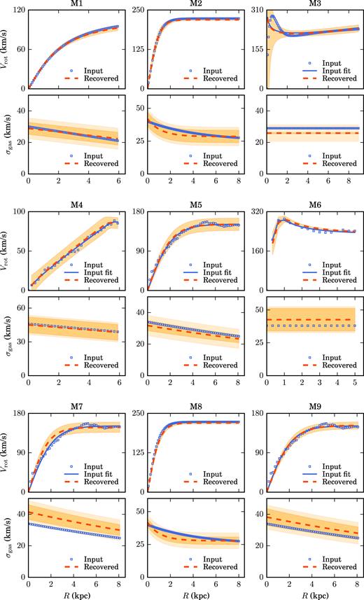
Rotation curves and velocity dispersions for the mock data set M1–M9. The blue squares are the input rotation curves and velocity dispersion profiles used to create the cubes containing the sources. These are then lensed forward to build the lensed mock data. The dashed red lines are the functional forms that best describe the kinematic priors, while the solid blue line for M3–M7 and M9 shows the fit to the input data using the same functional forms as those used for the kinematic priors at the 3D lens modelling stage. The orange bands for V_rot and σ_gas are obtained by error propagation from the uncertainties of the parameters that defined the rotation curves and velocity dispersion profiles, while the light orange bands for σ_gas take into account also the contribution from the spectral resolution (see Section 5 for further details). In the velocity dispersion profile of M3, the orange band is too thin (0.25 km s⁻¹) to be visible, see the Discussion in Section 5.3 for further details.

Open in new tab Download slide

Table 2.

Open in new tab

For each model in column 1, we show the assumptions on the input (second column) and recovered (third column) shapes for the rotation curves. The fourth and fifth columns show the median uncertainties on the lens and kinematic parameters. The sixth and seventh columns show the relative accuracies for the lens and kinematic parameters, respectively.

Mock data set	Input RC	Model RC	Median uncertainty	Median uncertainty	Median accuracy	Median accuracy
			on \|$\boldsymbol{\eta _{\mathrm{lens}}}$\|	on \|$\boldsymbol{\eta _{\mathrm{kin}}}$\|	on \|$\boldsymbol{\eta _{\mathrm{lens}}}$\|	on \|$\boldsymbol{\eta _{\mathrm{kin}}}$\|
			per cent	per cent	per cent	per cent
M1	Arctangent	Arctangent	2	7	3.6	2.3
M2	Hyperbolic	Hyperbolic	5	13	1.3	2.8
M3	Equation (26)	Multiparameter	5	3	2.8	1.7
M4	NGC 2976	Multiparameter	5	9	1.5	3.0
M5	NGC 3198	Hyperbolic	3	8	0.5	0.5
M6	NGC 6674	Multiparameter	6	9	1.0	1.1
M7	NGC 3198	Hyperbolic	8	6	2.4	3.1
	+ low inclination
M8	Hyperbolic	Hyperbolic	3	7	0.7	2.0
	+ large inclination
M9	NGC 3198	Hyperbolic	6	7	1.9	0.5
	+ warp

Mock data set	Input RC	Model RC	Median uncertainty	Median uncertainty	Median accuracy	Median accuracy
			on \|$\boldsymbol{\eta _{\mathrm{lens}}}$\|	on \|$\boldsymbol{\eta _{\mathrm{kin}}}$\|	on \|$\boldsymbol{\eta _{\mathrm{lens}}}$\|	on \|$\boldsymbol{\eta _{\mathrm{kin}}}$\|
			per cent	per cent	per cent	per cent
M1	Arctangent	Arctangent	2	7	3.6	2.3
M2	Hyperbolic	Hyperbolic	5	13	1.3	2.8
M3	Equation (26)	Multiparameter	5	3	2.8	1.7
M4	NGC 2976	Multiparameter	5	9	1.5	3.0
M5	NGC 3198	Hyperbolic	3	8	0.5	0.5
M6	NGC 6674	Multiparameter	6	9	1.0	1.1
M7	NGC 3198	Hyperbolic	8	6	2.4	3.1
	+ low inclination
M8	Hyperbolic	Hyperbolic	3	7	0.7	2.0
	+ large inclination
M9	NGC 3198	Hyperbolic	6	7	1.9	0.5
	+ warp

Table 2.

Open in new tab

For each model in column 1, we show the assumptions on the input (second column) and recovered (third column) shapes for the rotation curves. The fourth and fifth columns show the median uncertainties on the lens and kinematic parameters. The sixth and seventh columns show the relative accuracies for the lens and kinematic parameters, respectively.

Mock data set	Input RC	Model RC	Median uncertainty	Median uncertainty	Median accuracy	Median accuracy
			on \|$\boldsymbol{\eta _{\mathrm{lens}}}$\|	on \|$\boldsymbol{\eta _{\mathrm{kin}}}$\|	on \|$\boldsymbol{\eta _{\mathrm{lens}}}$\|	on \|$\boldsymbol{\eta _{\mathrm{kin}}}$\|
			per cent	per cent	per cent	per cent
M1	Arctangent	Arctangent	2	7	3.6	2.3
M2	Hyperbolic	Hyperbolic	5	13	1.3	2.8
M3	Equation (26)	Multiparameter	5	3	2.8	1.7
M4	NGC 2976	Multiparameter	5	9	1.5	3.0
M5	NGC 3198	Hyperbolic	3	8	0.5	0.5
M6	NGC 6674	Multiparameter	6	9	1.0	1.1
M7	NGC 3198	Hyperbolic	8	6	2.4	3.1
	+ low inclination
M8	Hyperbolic	Hyperbolic	3	7	0.7	2.0
	+ large inclination
M9	NGC 3198	Hyperbolic	6	7	1.9	0.5
	+ warp

Mock data set	Input RC	Model RC	Median uncertainty	Median uncertainty	Median accuracy	Median accuracy
			on \|$\boldsymbol{\eta _{\mathrm{lens}}}$\|	on \|$\boldsymbol{\eta _{\mathrm{kin}}}$\|	on \|$\boldsymbol{\eta _{\mathrm{lens}}}$\|	on \|$\boldsymbol{\eta _{\mathrm{kin}}}$\|
			per cent	per cent	per cent	per cent
M1	Arctangent	Arctangent	2	7	3.6	2.3
M2	Hyperbolic	Hyperbolic	5	13	1.3	2.8
M3	Equation (26)	Multiparameter	5	3	2.8	1.7
M4	NGC 2976	Multiparameter	5	9	1.5	3.0
M5	NGC 3198	Hyperbolic	3	8	0.5	0.5
M6	NGC 6674	Multiparameter	6	9	1.0	1.1
M7	NGC 3198	Hyperbolic	8	6	2.4	3.1
	+ low inclination
M8	Hyperbolic	Hyperbolic	3	7	0.7	2.0
	+ large inclination
M9	NGC 3198	Hyperbolic	6	7	1.9	0.5
	+ warp

The mock data M2 were built assuming an arctangent function for the rotation velocity (blue squares in Fig. 3). The data are modelled twice, once with the same functional form that we have used as input and the other with a hyperbolic tangent function.

We have created the simulated data M3 using the following functional form for the rotation velocity (blue squares in Fig. 3):

\begin{eqnarray*} V_{\mathrm{rot}}\left(R\right)=\sqrt{V_{1}^2+V_{2}^2}, \end{eqnarray*}

(26)

where V₁ is the contribution from an isothermal dark-matter halo while V₂ represents the contribution from a Sérsic profile with a Sérsic index n = 1 (Freeman 1970). Since our lens modelling code does not include the functional form expressed by equation (26), we model these mock data using the flexible multiparameter function (dashed red line in Fig. 3). After checking that the input rotation curve is well reproduced (see the Discussion in Section 5.3 for further details), we fit the input 1D rotation curve with the multiparameter function (blue solid line in Fig. 3).¹ By comparing the results of this fit with the kinematic parameters derived by the 3D lens modelling code, we can then quantify the accuracy of our technique and study the systematic errors that may derive from the choice of the kinematic functional forms.

We have created the mock data sets M4, M5, and M6 using the rotation curves measured for three low-redshift galaxies: NGC 2976, NGC 3198, and NGC 6674 from Lelli, McGaugh & Schombert (2016). For these sources, the values of the rotation parameters listed in Table 1 are obtained by fitting the input data points (blue squares in Fig. 3) with one of the functional forms implemented in our code (blue solid line in Fig. 3). As for M2, this fitting allows us to evaluate an accuracy of the inferred kinematic parameters which is independent of the choice of the parametrization. As discussed in Sections 5.4–5.6, these mock data are then modelled assuming the multiparameter function for M4 and M6 and the hyperbolic tangent function for M5.

The simulated data M7, M8, and M9 are built to test the limits of our method. M7 and M8 have the same kinematics of M5 and M2 but an inclination angle of 40° and 80°, respectively. M9 has the same kinematics of M5, but it has a strong warp, which causes a change of 30° of its position angle across the galaxy.

5 RESULTS

To test the ability of our method to recover the input lens and kinematic parameters, we model the nine mock data sets introduced in Section 3.2 with the new modelling technique described in Section 2.1. All assumptions made during the modelling procedure were discussed in Section 4.

We obtain the uncertainties on the inferred parameters using multinest (see Section 2.4). For each parameter, we adopt priors that are flat in the intervals |$[\boldsymbol{\overline{\eta }_{\mathrm{lens/kin}}}-0.2\boldsymbol{\overline{\eta }_{\mathrm{lens/kin}}}, \boldsymbol{\overline{\eta }_{\mathrm{lens/kin}}}+0.2\boldsymbol{\overline{\eta }_{\mathrm{lens/kin}}}]$|⁠, where |$\boldsymbol{\overline{\eta }_{\mathrm{lens/kin}}}$| are the best-fitting parameters, inferred from the non-linear optimization (see Section 2.1). To be conservative, we report as errors in the parameters the sum in quadrature of the following two contributions: the 1σ uncertainties on the posterior distributions derived by multinest and the difference between the maximum a posteriori parameter values obtained by multinest, and the non-linear optimizer. This difference arises because, as discussed above, the geometrical parameters that describe the source, i.e. PA and i, are kept fixed during the optimization, while they are left free to vary during the multinest exploration of the parameter space. In most cases, the discrepancy is smaller than 5 per cent, while it reaches a level of 20 per cent in one case that will be discussed separately (see Section 5.6). For the mock data M1, M2, and M8, for which we have used the same functional forms to create and model the data, these errors only account for the statistical uncertainties, while for the other models they also provide an estimate of the systematic errors, related to the choice of parametrization. The median relative uncertainties on |$\boldsymbol{\eta _{\mathrm{lens}}}$| and |$\boldsymbol{\eta _{\mathrm{kin}}}$| for each model are listed in Table 2 (fourth and fifth columns, respectively), while the sixth and seventh columns in Table 2 list the relative accuracies.²

Figs. 5 (for M1) and B1–B8 in Appendix B (for M2–M8) show the comparison between mock observations and best-fitting models. We plot the contour levels of the input source (first column), the simulated lensed data (second column), the inferred lensed model (third column), the normalized image residuals (fourth column), the reconstructed source (fifth column), and the contour levels of the kinematic model (sixth column), for a selected number of spectral channels. We present the input and recovered rotation curves and velocity dispersion profiles with blue squares and dashed red lines, respectively, in Fig. 3. The orange band for the rotation velocities denotes the uncertainties ε_p, obtained after propagating the uncertainties on the parameters that describe the profiles (see Table 3). To take into account the contribution to the velocity dispersion uncertainties due to the spectral resolution, we compute the uncertainties on the values of σ(R) as |$\sqrt{\epsilon _{\mathrm{p}}^2+\epsilon _{\mathrm{cw}}^2}$| (light orange bands in Fig. 3). ε_p (orange bands in Fig. 3) has the same meaning defined above for V_rot(R), while ε_cw is obtained as the FWHM of the channel width divided by 3 × 2.355. The factor of 3 is obtained after testing the effect of the spectral resolution on the recovered velocity dispersion with mock data. We list the inferred lens and kinematic parameters in Table 3. These values should be compared with those reported in Table 1.

Table 3.

Open in new tab

Top table: Recovered kinematic parameters that best describe the prior for the nine sources. Bottom table: Recovered lens parameters for the nine mock data sets. The uncertainties are derived using a multinest method, as explained in Section 5.

Recovered kinematic parameters
Mock data set	i	PA	V_t	R_t	β	ξ	σ₀	R₀	σ₁
	°	°	km s⁻¹	kpc			km s⁻¹	kpc	km s⁻¹
M1	74.0 ± 1.6	260.0 ± 3.2	115.0 ± 4.8	1.86 ± 0.23	–	–	28.9 ± 3.7	−1.1 ± 0.23	–
M2	54.4 ± 0.1	102.6 ± 2.7	219.3 ± 2.2	0.97 ± 0.09	–	–	13.4 ± 2.6	1.15 ± 0.21	28.5 ± 4.6
M3	63.2 ± 0.4	24.6 ± 1.5	155.4 ± 4.2	27.1 ± 5.2	1.09 ± 0.02	95.8 ± 13.1	25.9 ± 0.25	–	–
M4	60.0 ± 1.8	150.0 ± 5.6	72.9 ± 5.6	5.23 ± 0.53	0.25 ± 0.03	51.4 ± 5.3	43.9 ± 6.8	−1.13 ± 0.20	–
M5	70.7 ± 5.9	282.9 ± 2.5	151.2 ± 13.9	2.07 ± 0.18	–	–	31.8 ± 3.2	26.2 ± 2.1	–
M6	62.0 ± 3.3	45.0 ± 4.2	220.9 ± 1.2	0.75 ± 0.13	0.57 ± 0.03	4.80 ± 1.70	42.6 ± 8.5	–	–
M7	40.2 ± 0.5	281.4 ± 2.7	151.2 ± 11.4	2.09 ± 0.13	–	–	41.1 ± 4.6	24.9 ± 1.8	–
M8	81.2 ± 2.5	97.5 ± 3.8	219.7 ± 2.4	1.07 ± 0.09	–	–	13.9 ± 1.0	1.12 ± 0.12	27.8 ± 2.8
M9	67.6 ± 6.3	277.8 ± 2.7/−3.3 ± 1.9	152.4 ± 7.8	2.23 ± 0.18	–	–	38.2 ± 5.8	25.9 ± 2.6	–
Recovered lens parameters
Mock data set	κ₀	θ	q	γ	Γ_sh	θ_sh
	arcsec	°				°
M1	1.43 ± 0.01	−15.6 ± 0.5	0.79 ± 0.02	2.05 ± 0.01	−0.044 ± 0.004	10.2 ± 0.8
M2	1.34 ± 0.05	155.8 ± 4.9	0.95 ± 0.06	2.25 ± 0.10	0.056 ± 0.011	173.38 ± 0.11
M3	0.97 ± 0.04	−0.08 ± 0.01	0.98 ± 0.01	2.04 ± 0.06	0.257 ± 0.025	39.1 ± 0.07
M4	1.31 ± 0.09	160.50 ± 6.5	0.95 ± 0.01	2.31 ± 0.16	0.051 ± 0.009	173.8 ± 6.8
M5	0.78 ± 0.03	69.6 ± 0.4	0.83 ± 0.06	2.03 ± 0.04	0.096 ± 0.002	34.3 ± 3.2
M6	1.43 ± 0.01	−15.65 ± 2.7	0.82 ± 0.03	2.08 ± 0.12	−0.037 ± 0.001	14.76 ± 1.19
M7	0.83 ± 0.04	72.1 ± 6.2	0.81 ± 0.07	1.96 ± 0.09	0.093 ± 0.002	33.3 ± 3.1
M8	1.32 ± 0.02	153.7 ± 4.5	0.96 ± 0.03	2.28 ± 0.02	0.056 ± 0.004	173.2 ± 4.1
M9	0.82 ± 0.07	72.6 ± 4.4	0.82 ± 0.02	1.99 ± 0.13	0.101 ± 0.004	33.9 ± 1.7

Recovered kinematic parameters
Mock data set	i	PA	V_t	R_t	β	ξ	σ₀	R₀	σ₁
	°	°	km s⁻¹	kpc			km s⁻¹	kpc	km s⁻¹
M1	74.0 ± 1.6	260.0 ± 3.2	115.0 ± 4.8	1.86 ± 0.23	–	–	28.9 ± 3.7	−1.1 ± 0.23	–
M2	54.4 ± 0.1	102.6 ± 2.7	219.3 ± 2.2	0.97 ± 0.09	–	–	13.4 ± 2.6	1.15 ± 0.21	28.5 ± 4.6
M3	63.2 ± 0.4	24.6 ± 1.5	155.4 ± 4.2	27.1 ± 5.2	1.09 ± 0.02	95.8 ± 13.1	25.9 ± 0.25	–	–
M4	60.0 ± 1.8	150.0 ± 5.6	72.9 ± 5.6	5.23 ± 0.53	0.25 ± 0.03	51.4 ± 5.3	43.9 ± 6.8	−1.13 ± 0.20	–
M5	70.7 ± 5.9	282.9 ± 2.5	151.2 ± 13.9	2.07 ± 0.18	–	–	31.8 ± 3.2	26.2 ± 2.1	–
M6	62.0 ± 3.3	45.0 ± 4.2	220.9 ± 1.2	0.75 ± 0.13	0.57 ± 0.03	4.80 ± 1.70	42.6 ± 8.5	–	–
M7	40.2 ± 0.5	281.4 ± 2.7	151.2 ± 11.4	2.09 ± 0.13	–	–	41.1 ± 4.6	24.9 ± 1.8	–
M8	81.2 ± 2.5	97.5 ± 3.8	219.7 ± 2.4	1.07 ± 0.09	–	–	13.9 ± 1.0	1.12 ± 0.12	27.8 ± 2.8
M9	67.6 ± 6.3	277.8 ± 2.7/−3.3 ± 1.9	152.4 ± 7.8	2.23 ± 0.18	–	–	38.2 ± 5.8	25.9 ± 2.6	–
Recovered lens parameters
Mock data set	κ₀	θ	q	γ	Γ_sh	θ_sh
	arcsec	°				°
M1	1.43 ± 0.01	−15.6 ± 0.5	0.79 ± 0.02	2.05 ± 0.01	−0.044 ± 0.004	10.2 ± 0.8
M2	1.34 ± 0.05	155.8 ± 4.9	0.95 ± 0.06	2.25 ± 0.10	0.056 ± 0.011	173.38 ± 0.11
M3	0.97 ± 0.04	−0.08 ± 0.01	0.98 ± 0.01	2.04 ± 0.06	0.257 ± 0.025	39.1 ± 0.07
M4	1.31 ± 0.09	160.50 ± 6.5	0.95 ± 0.01	2.31 ± 0.16	0.051 ± 0.009	173.8 ± 6.8
M5	0.78 ± 0.03	69.6 ± 0.4	0.83 ± 0.06	2.03 ± 0.04	0.096 ± 0.002	34.3 ± 3.2
M6	1.43 ± 0.01	−15.65 ± 2.7	0.82 ± 0.03	2.08 ± 0.12	−0.037 ± 0.001	14.76 ± 1.19
M7	0.83 ± 0.04	72.1 ± 6.2	0.81 ± 0.07	1.96 ± 0.09	0.093 ± 0.002	33.3 ± 3.1
M8	1.32 ± 0.02	153.7 ± 4.5	0.96 ± 0.03	2.28 ± 0.02	0.056 ± 0.004	173.2 ± 4.1
M9	0.82 ± 0.07	72.6 ± 4.4	0.82 ± 0.02	1.99 ± 0.13	0.101 ± 0.004	33.9 ± 1.7

Table 3.

Open in new tab

Top table: Recovered kinematic parameters that best describe the prior for the nine sources. Bottom table: Recovered lens parameters for the nine mock data sets. The uncertainties are derived using a multinest method, as explained in Section 5.

Recovered kinematic parameters
Mock data set	i	PA	V_t	R_t	β	ξ	σ₀	R₀	σ₁
	°	°	km s⁻¹	kpc			km s⁻¹	kpc	km s⁻¹
M1	74.0 ± 1.6	260.0 ± 3.2	115.0 ± 4.8	1.86 ± 0.23	–	–	28.9 ± 3.7	−1.1 ± 0.23	–
M2	54.4 ± 0.1	102.6 ± 2.7	219.3 ± 2.2	0.97 ± 0.09	–	–	13.4 ± 2.6	1.15 ± 0.21	28.5 ± 4.6
M3	63.2 ± 0.4	24.6 ± 1.5	155.4 ± 4.2	27.1 ± 5.2	1.09 ± 0.02	95.8 ± 13.1	25.9 ± 0.25	–	–
M4	60.0 ± 1.8	150.0 ± 5.6	72.9 ± 5.6	5.23 ± 0.53	0.25 ± 0.03	51.4 ± 5.3	43.9 ± 6.8	−1.13 ± 0.20	–
M5	70.7 ± 5.9	282.9 ± 2.5	151.2 ± 13.9	2.07 ± 0.18	–	–	31.8 ± 3.2	26.2 ± 2.1	–
M6	62.0 ± 3.3	45.0 ± 4.2	220.9 ± 1.2	0.75 ± 0.13	0.57 ± 0.03	4.80 ± 1.70	42.6 ± 8.5	–	–
M7	40.2 ± 0.5	281.4 ± 2.7	151.2 ± 11.4	2.09 ± 0.13	–	–	41.1 ± 4.6	24.9 ± 1.8	–
M8	81.2 ± 2.5	97.5 ± 3.8	219.7 ± 2.4	1.07 ± 0.09	–	–	13.9 ± 1.0	1.12 ± 0.12	27.8 ± 2.8
M9	67.6 ± 6.3	277.8 ± 2.7/−3.3 ± 1.9	152.4 ± 7.8	2.23 ± 0.18	–	–	38.2 ± 5.8	25.9 ± 2.6	–
Recovered lens parameters
Mock data set	κ₀	θ	q	γ	Γ_sh	θ_sh
	arcsec	°				°
M1	1.43 ± 0.01	−15.6 ± 0.5	0.79 ± 0.02	2.05 ± 0.01	−0.044 ± 0.004	10.2 ± 0.8
M2	1.34 ± 0.05	155.8 ± 4.9	0.95 ± 0.06	2.25 ± 0.10	0.056 ± 0.011	173.38 ± 0.11
M3	0.97 ± 0.04	−0.08 ± 0.01	0.98 ± 0.01	2.04 ± 0.06	0.257 ± 0.025	39.1 ± 0.07
M4	1.31 ± 0.09	160.50 ± 6.5	0.95 ± 0.01	2.31 ± 0.16	0.051 ± 0.009	173.8 ± 6.8
M5	0.78 ± 0.03	69.6 ± 0.4	0.83 ± 0.06	2.03 ± 0.04	0.096 ± 0.002	34.3 ± 3.2
M6	1.43 ± 0.01	−15.65 ± 2.7	0.82 ± 0.03	2.08 ± 0.12	−0.037 ± 0.001	14.76 ± 1.19
M7	0.83 ± 0.04	72.1 ± 6.2	0.81 ± 0.07	1.96 ± 0.09	0.093 ± 0.002	33.3 ± 3.1
M8	1.32 ± 0.02	153.7 ± 4.5	0.96 ± 0.03	2.28 ± 0.02	0.056 ± 0.004	173.2 ± 4.1
M9	0.82 ± 0.07	72.6 ± 4.4	0.82 ± 0.02	1.99 ± 0.13	0.101 ± 0.004	33.9 ± 1.7

Recovered kinematic parameters
Mock data set	i	PA	V_t	R_t	β	ξ	σ₀	R₀	σ₁
	°	°	km s⁻¹	kpc			km s⁻¹	kpc	km s⁻¹
M1	74.0 ± 1.6	260.0 ± 3.2	115.0 ± 4.8	1.86 ± 0.23	–	–	28.9 ± 3.7	−1.1 ± 0.23	–
M2	54.4 ± 0.1	102.6 ± 2.7	219.3 ± 2.2	0.97 ± 0.09	–	–	13.4 ± 2.6	1.15 ± 0.21	28.5 ± 4.6
M3	63.2 ± 0.4	24.6 ± 1.5	155.4 ± 4.2	27.1 ± 5.2	1.09 ± 0.02	95.8 ± 13.1	25.9 ± 0.25	–	–
M4	60.0 ± 1.8	150.0 ± 5.6	72.9 ± 5.6	5.23 ± 0.53	0.25 ± 0.03	51.4 ± 5.3	43.9 ± 6.8	−1.13 ± 0.20	–
M5	70.7 ± 5.9	282.9 ± 2.5	151.2 ± 13.9	2.07 ± 0.18	–	–	31.8 ± 3.2	26.2 ± 2.1	–
M6	62.0 ± 3.3	45.0 ± 4.2	220.9 ± 1.2	0.75 ± 0.13	0.57 ± 0.03	4.80 ± 1.70	42.6 ± 8.5	–	–
M7	40.2 ± 0.5	281.4 ± 2.7	151.2 ± 11.4	2.09 ± 0.13	–	–	41.1 ± 4.6	24.9 ± 1.8	–
M8	81.2 ± 2.5	97.5 ± 3.8	219.7 ± 2.4	1.07 ± 0.09	–	–	13.9 ± 1.0	1.12 ± 0.12	27.8 ± 2.8
M9	67.6 ± 6.3	277.8 ± 2.7/−3.3 ± 1.9	152.4 ± 7.8	2.23 ± 0.18	–	–	38.2 ± 5.8	25.9 ± 2.6	–
Recovered lens parameters
Mock data set	κ₀	θ	q	γ	Γ_sh	θ_sh
	arcsec	°				°
M1	1.43 ± 0.01	−15.6 ± 0.5	0.79 ± 0.02	2.05 ± 0.01	−0.044 ± 0.004	10.2 ± 0.8
M2	1.34 ± 0.05	155.8 ± 4.9	0.95 ± 0.06	2.25 ± 0.10	0.056 ± 0.011	173.38 ± 0.11
M3	0.97 ± 0.04	−0.08 ± 0.01	0.98 ± 0.01	2.04 ± 0.06	0.257 ± 0.025	39.1 ± 0.07
M4	1.31 ± 0.09	160.50 ± 6.5	0.95 ± 0.01	2.31 ± 0.16	0.051 ± 0.009	173.8 ± 6.8
M5	0.78 ± 0.03	69.6 ± 0.4	0.83 ± 0.06	2.03 ± 0.04	0.096 ± 0.002	34.3 ± 3.2
M6	1.43 ± 0.01	−15.65 ± 2.7	0.82 ± 0.03	2.08 ± 0.12	−0.037 ± 0.001	14.76 ± 1.19
M7	0.83 ± 0.04	72.1 ± 6.2	0.81 ± 0.07	1.96 ± 0.09	0.093 ± 0.002	33.3 ± 3.1
M8	1.32 ± 0.02	153.7 ± 4.5	0.96 ± 0.03	2.28 ± 0.02	0.056 ± 0.004	173.2 ± 4.1
M9	0.82 ± 0.07	72.6 ± 4.4	0.82 ± 0.02	1.99 ± 0.13	0.101 ± 0.004	33.9 ± 1.7

In Fig. 4, we show the comparison between the input and recovered flat velocities V_flat and average velocity dispersions 〈σ_gas〉. The values of V_flat are obtained as the average of the rotation velocities at large radii, while the 〈σ_gas〉 are obtained by averaging the values of σ_gas(R) starting from R = 0 kpc. The error bars in Fig. 4 take into account the contribution of both the uncertainties on the values of V_rot and σ_gas at each radius, as showed by the orange and light orange bands in Fig. 3, and the standard deviation. The flat part of the rotation curves is correctly reproduced for all mock data sets. In particular, with our technique, we are able to recover V_flat not only for the galaxies for which the input rotation curves are described by functional forms, but also for the rotation curves taken from real galaxies. This test ensures that the functional forms implemented in our code are flexible enough to reproduce the variety of shape of rotation curves (from dwarf to massive galaxies). Even if the details in the inner region could be lost (see Section 5.3), the physical parameters that depend on V_flat can be exactly recovered. The values of 〈σ_gas〉 are recovered with a great accuracy, even if they are more affected by the spectral resolution.

Figure 4.

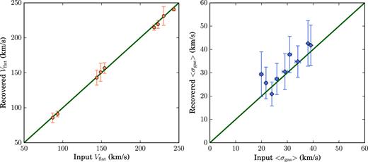
Left: Recovered versus input values of V_flat for the nine mock data sets. Some points are shifted both on x- and y-axis by the same quantity for a better visualization of all the points. The green line represents a 1:1 relation between quantities on x- and y-axis. Right: Same as in the left-hand panel, but for 〈σ_gas〉. The errors bars take into account both the standard uncertainties due to error propagation and the standard deviation due to fact that these are averaged quantities.

Open in new tab Download slide

Figure 5.

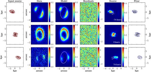
The rows show some representative channel maps for the simulated data set M1. Column 1: Input source. Column 2: Mock lensed data. Column 3: Lensed model and the corresponding critical curves. Column 4: Normalized residuals obtained as the ratio between the difference of the data and the model and the corresponding noise. Column 5: Reconstructed source and caustics. Column 6: Kinematic prior used to constrain the source reconstruction. The contour levels in the first and sixth columns are set at n = 0.1, 0.2, 0.4, 0.6, 0.8 times the value of the maximum flux.

Open in new tab Download slide

Below, we provide a detailed discussion on the modelling results for each of the nine simulated data sets. The reader not interested in the details can skip to Section 5.10, where we address some key issues related to radial motions, SNRs, and changes in the centre coordinates and systemic velocities and to Section 6 where we summarize the results of our tests.

5.1 Mock data set M1

The simulated data M1 were created assuming an arctangent function for the rotation velocity and a dispersion curve that is linearly declining from a value of 30 km s⁻¹ at R = 0 kpc to 21 km s⁻¹ at R = 5.9 kpc. The source position angle also changes linearly from 270° in the inner regions to 260° in the outer areas.

We model the simulated data with the same functional forms used to create them. Since the small change in the position angle is not detectable by a visual analysis of the zeroth-moment map, resulting from the first step of the optimization scheme (see Section 2.4), we decided to keep it fixed to the constant value of 260° during the following steps. We have found that this assumption does not significantly influence the derived kinematics. The inferred parameters that define the rotation velocity and the velocity dispersion have median relative uncertainties of 7 per cent and are within 2σ from the input values. The inferred lens parameters, characterized by median relative uncertainties of 2 per cent, are within 1σ from the input values, with the only exceptions of the lens and external-shear position angles θ and θ_sh that differ by 5.7σ and 3.9σ, respectively, from the input values. This result is related to the fact that the lens is very close to being spherical and the shear strength almost negligible.

5.2 Mock data set M2

We have created the simulated data M2 using a hyperbolic tangent function for the source rotation curve and an exponential function for its velocity dispersion.

First, we model this data set assuming the same functional forms used as input. This choice produces normalized residuals that are of the order of 0.5 per cent (see the fourth column in Fig. B1). The inferred lens parameters have a median relative uncertainty of 5 per cent, while the recovered kinematic parameters have median relative uncertainties of 13 per cent (Table 3). The largest contribution to the kinematic uncertainties comes from the velocity dispersion parameters, due to the limited spectral resolution (channel width of ∼36.8 km s⁻¹) of these data (see the orange band in Fig. 3). The input lens and the kinematic parameters are within the 1σ uncertainties from the recovered values. To test our capability to distinguish between different forms of parametrization, we have also modelled this data set with an arctangent function. We have found that under this assumption the residuals get worse (see the third column in Fig. 6), reaching a maximum value of ∼6σ. We have then computed the marginalized Bayesian evidence to compare and rank these two models. As anticipated in Section 2.4, the marginalized evidence in equation (14) allows us to quantify how well a model m_i is supported by the data against another model m_j. This quantification is expressed in terms of the Bayes factor, Δlog E_ij = log E_i − log E_j. We find that the Bayes factor is of the order of 1400 against the arctangent model, meaning that the hyperbolic tangent function for the rotation curve is largely supported by the data. We can conclude, therefore, that the data contain enough information for us to infer the most suitable shape.

Figure 6.

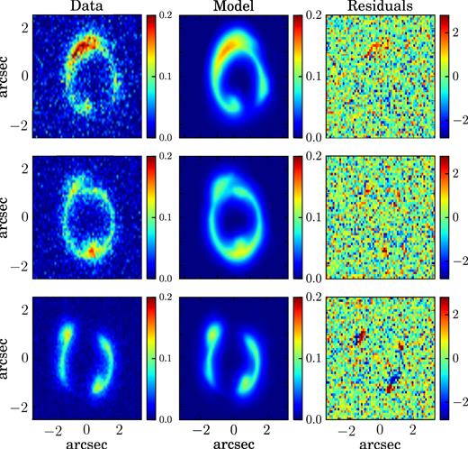
Same as Fig. B1, for a rotation velocity described by an arctangent function.

Open in new tab Download slide

5.3 Mock data set M3

The lens system M3 was created assuming a rotation curve for the background galaxy described by the functional form in equation (26). This function is not implemented in our code. The velocity dispersion was assumed to be constant.

We model these simulated data using the multiparameter function given by equation (20), which is the most flexible function that we have implemented. We find that the lens parameters are recovered with a median relative uncertainty of 5 per cent and are within 1σ from the input values. Our constraints on the lens–mass model are therefore not significantly influenced by our assumptions on the source prior. The inferred parameters that define the rotation curve (V_t, R_t, β, ξ) in Table 3 should be compared with those reported in Table 1, obtained by fitting the input 1D rotation curve (blue squares in Fig. 3) using the multiparameter function (solid blue line in Fig. 3). The inferred kinematic parameters have median uncertainties of 3 per cent and they are within 2σ from the fitted values. The only exception is the recovered velocity dispersion that is more than 3σ away. However, this discrepancy is due to an underestimation of the uncertainties that do not include the systematic errors introduced by the spectral resolution. If we take into account the uncertainties due to spectral resolution, ε_cw in Section 5, the recovered dispersion profile is in agreement within 1σ with the input profile (see the light orange band in Fig. 3). We find that both the fit to the input rotation curve (solid blue line in Fig. 3) and the rotation curve derived from our lens modelling technique (red dashed line in Fig. 3) are a poor description of the inner regions of the real curve (see the blue squares in Fig. 3). Despite its flexibility, the multiparameter function does not allow us to correctly reproduce the peculiarity of the data in the central regions. Correspondingly, we find that the overall fit to the data has systematic residuals that reach maximum values of ∼5σ (see the third column in Fig. B2). However, the rotation velocity at the outer regions is well reproduced, ensuring that even if the details of the inner regions are lost, the physical parameters that depend on the asymptotic velocity (e.g. angular momentum and dynamical mass) can still be recovered with good accuracy (see Fig. 4).

5.4 Mock data set M4

The input values of the rotation velocity for this system are taken from the rotation curve of the nearby dwarf galaxy NGC 2976 (Lelli et al. 2016). This choice allows us to test whether the assumed functional forms are good enough to reproduce real rotational curves. A linear equation describes the velocity dispersion curve.

During the modelling phase, we use the multiparameter function, equation (20), to describe the rotation velocity, while for the velocity dispersion we use the same functional form used as input. As for the simulated data M3, to have a quantitative estimate of the accuracy on the derived kinematics, we first fit the input 1D rotation curve with the same functional form used in the 3D lens modelling process (solid blue line in Fig. 3). The recovered kinematic parameters have a median relative uncertainty of 9 per cent, while the lens parameters have a median relative uncertainty of 5 per cent (Table 3). The inferred lens parameters are within the 2σ errors from the input values. The kinematic parameters are within 1σ from the values derived by fitting the 1D rotation curve.

5.5 Mock data set M5

As for the simulated data set M4, we create M5 using the rotation curve of a real galaxy as input, in this case NGC 3198 (Lelli et al. 2016). The input functional form for the velocity dispersion is an exponential function, equation (23), with σ₁ = 0.0 km s⁻¹.

At the modelling stage, we use the hyperbolic tangent function for the rotation curve and an exponential function with σ₁ fixed at zero km s⁻¹ for the velocity dispersion. As for the simulated data M3 and M4, we start by fitting the 1D rotation curve with the same functional form used for the 3D lens modelling. We find that the hyperbolic tangent function provides a good enough description of the data. The normalized residuals (fourth column in Fig. B4), indeed, do not show any systematic features, usually indicative of wrong assumptions in the building of the prior (e.g. see the models M2 and M3 in Sections 5.2 and 5.3). The recovered lens and kinematic parameters have median relative uncertainties of 3 and 8 per cent, respectively, and they are within 1σ from the input values.

5.6 Mock data set M6

The simulated data M6 were created using the rotation curve of the nearby galaxy NGC 6674 (Lelli et al. 2016), while for the velocity dispersion curve we have used a constant value of 38 km s⁻¹. When modelling the data, the prior is built assuming the multiparameter function for the rotation curve, while the dispersion is assumed to be constant.

The input lens parameters (Table 1) are within the 1σ uncertainties from the recovered values (Table 3). The kinematic parameters inferred by the 3D lens modelling technique are within 1σ from the values derived by fitting the 1D rotation curve directly. We find that the inferred lens and kinematic parameters have a median relative uncertainty of 6 and 9 per cent, respectively. In particular, the velocity dispersion, σ₀, has an uncertainty of 20 per cent. The major contribution to this error is the difference between the maximum a posteriori parameter value of 51.1 km s⁻¹ obtained by multinest and the corresponding value of 42.6 km s⁻¹ obtained by the non-linear optimizer (see Section 5). However, given the channel width of 33.9 km s⁻¹ for this system, we believe the discrepancy not to be significant.

5.7 Mock data set M7

The derivation of the rotation curve for low-inclination galaxies is challenging for any kinematic-fitting algorithm. For example, for i = 40°, an error as small as ±5° in the estimation of the inclination angle can lead to a significant underestimation/overestimation of the rotation velocity as large as 10 per cent. To test the reliability of our modelling technique when the background source is a low-inclination galaxy, we have created the mock data M7 with the same lens and kinematic parameters of M5, but with an inclination angle for the source of 40°, instead of 68°.

As described above, we first model the zeroth-moment map and then use the recovered lens model parameters to derive a 3D model of the source. The latter is then analysed with ^3Dbarolo to obtain initial guesses for the source geometrical parameters. For the mock data M7, this results in a value of i = 41.5°, in close agreement with the input value. Subsequently, by applying our 3D lens modelling analysis to the full lensed data cube, we derive an inclination angle of 40.2°. The inferred lens and kinematic parameters have median relative uncertainties of 8 and 6 per cent, respectively, differing by 1σ and 2σ from the input values. We can conclude, therefore, that the accurate reconstruction of the zeroth-moment map allows us to obtain a reasonable initial estimate of the inclination and, as a consequence, the kinematic properties of the galaxy are correctly recovered.

5.8 Mock data set M8

Di Teodoro & Fraternali (2015) have shown that for large inclinations, i > 75°, the inner points of the rotation curve can be underestimated and that this effect can be more significant for a flat rather than for a solid-body rotation curve. This is due to the fact that ^3Dbarolo works ring by ring. However, we note that for a value of the inclination angle >75°, the errors on the inclination have little impact on the derived rotation curve, due to the sinusoidal dependence between the line-of-sight velocity and the inclination, see equation (17).

These mock data were built to study how an extreme value of the inclination angle affects the reconstruction of the source kinematics. For this reason, we have built the mock data M8 using the same lens and kinematic models as those used for M2, but assuming an inclination angle of 80°. In particular, we focus on M2 because it has a flat rotation curve.

The inferred values that describe the rotation velocity differ by ∼4 per cent from the input values, reproducing very well also the inner regions of the curve (see the red dashed line in Fig. 3). We can conclude, therefore, that the use of functional forms for the rotation velocity allows us to reproduce the inner regions of an edge-on galaxy better than a ring by ring method. Moreover, the inferred lens and kinematic parameters are characterized by median relative uncertainties of 3 and 7 per cent, respectively, and they are within 2σ from the input values.

5.9 Mock data set M9

The input lens and kinematic models are the same as those used to create the simulated data M5, but the input geometry of the source is different. In particular, the position angle has a strong warp, and it decreases linearly from a value of 280° at R = 0 kpc to 250° at the outermost radius.

Interestingly, we find that the presence of the warp is already revealed at the first step of our optimization strategy (Fig. 7), where we focus on the lens modelling of the zeroth moment [i.e. point (i), Section 2.4]. From a ^3Dbarolo analysis of the derived source cube, we then obtain a position angle that changes linearly with a slope of 2.6° kpc⁻¹ from an inner value of 278°. We then apply our 3D lens modelling technique with a position angle that changes linearly. The two parameters that describe this change are left free to vary, starting from the initial guesses found by ^3Dbarolo. The best-fitting slope that describes the variation of the PA is 3.3° kpc⁻¹, which differs by ∼6 per cent from the input value of 3.5° kpc⁻¹. The inferred value of PA at R = 0 kpc is 277.8°, differing by ∼1 per cent from the input value of 280.0°. The inferred kinematic parameters have a median uncertainty of 7 per cent, while the lens parameters have a median uncertainty of 6 per cent. Both the lens and the kinematic parameters are within 1σ from the input values.

Figure 7.

Zeroth-moment map for the reconstructed source M9, resulting after the first step [i.e. point (i), Section 2.4] of our optimization strategy.

Open in new tab Download slide

5.10 Further tests

Observational evidence seems to indicate that physical processes such as disc turbulence, gas accretion, and subsequent disc instabilities are more prevalent at high redshift (e.g. Förster Schreiber et al. 2006; Law et al. 2009; Wisnioski et al. 2015). As a consequence, the contribution of non-rotational components could have a significant impact on the kinematic of high-redshift galaxies. The presence of significant radial motions, which are not included in the current analysis, could, in principle, limit the applicability of our technique to high-|$z$| galaxies. To quantify this issue, we have created a simulated data set that has the same lens and kinematic models as M1 but includes radial motions of 25 km s⁻¹. We note that this value is larger than what is typically observed at low redshift (i.e. ≲10 km s⁻¹; Trachternach et al. 2008), while, to date, there are no studies of radial motion in high-redshift galaxies. We have compared the lensed images of these simulated data with those of M1 for different values of angular resolution. Even in the ideal case of no observational noise, we have found no significant discrepancy, with a relative difference between the two lensed images of the order of ∼2 per cent, for the highest angular resolution case. We can conclude that, although non-circular motions could contribute to the overall kinematics, they are mostly not detectable at the current angular and spectral resolution.

To test how the SNR of the data affects the accuracy with which the lens–mass and source–kinematic parameters are recovered, we have re-simulated the mock data M1 with five different noise levels, obtained using different exposure times (see Fig. A2 in Appendix A). As shown in the left-hand panel of Fig. 8, for an SNR³ below ∼3, the relative difference between the input and the recovered values is higher than 30 per cent both for the lens (orange circles) and for the kinematic parameters (magenta empty squares). If we focus on the relative difference between the input and the output V_flat (green triangles on the right-hand panel of Fig. 8), we conclude that we are still able to recover it with an accuracy of the order of 90 per cent even for the mock data set with the lowest SNR. The relative differences between the input and the recovered values of 〈σ_gas〉 (blue empty diamonds on the right-hand panel of Fig. 8) are smaller than ∼30 per cent for an SNR larger than 3.

Figure 8.

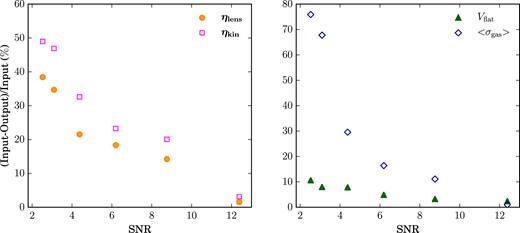
Left: Relative difference between the input and the recovered lens (orange circles) and kinematic (magenta empty squares) parameters as a function of the SNR for different data-quality realizations of M1 mock data set. Right: Same as in the left-hand panel but for V_flat (green triangles) and 〈σ_gas〉 (blue empty diamonds).

Open in new tab Download slide

So far, we have modelled all the simulated data sets with a fixed systemic velocity of zero km s⁻¹ and the centre of the kinematic prior set at the flux-weighted average position of the zeroth-moment map. However, for high-redshift galaxies, one expects an error on the centre of the order of 5–10 per cent and on the systemic velocity of the order of the channel width. We have, therefore, repeated the analysis of M1 by fixing the coordinates of the centre to values that are offset from the real ones by 10 per cent and with values of the systemic velocity that are offset by the channel width velocity from the real value. We have found that an incorrect choice of the systemic velocity does not affect our results significantly, while changes in the centre have a significant effect only if both coordinates are shifted by 10 per cent relative to the real values in the same direction.

Because of the small FOV of many IFU instruments, complete imaging of the lensed emission is often not possible, instead, only a limited part of the arc is observed. Here, we show how this observational limitation can strongly affect the reconstruction of the source morphology. The first row of Fig. 9 shows the emission of a background disc galaxy as lensed by a power-law mass distribution. In the same figure, we present the source that is reconstructed by considering an increasingly smaller part of the data. In particular, on the second row, we have modelled the entire set of images, on the third one we have excluded the counter image, on the fourth we have modelled only a small region of the main arc and the counter image, while on the fifth one only a small region of the main arc was taken into account. We find that one can safely ignore the counter image only if all images are modelled (see the third row of Fig. 9). However, failure to observe the entire main arc leads to an incorrect source reconstruction and a wrong estimate of both the centre of the galaxy and its extension, strongly affecting the derived kinematics (see the fifth row of Fig. 9). In this case, including the counter image is fundamental for a better reconstruction of the source (see the fourth row in Fig. 9). This result is due to the extension of the source, such that different regions of the galaxy are lensed into different regions and/or number of the images, depending on the lens system configuration. We conclude, therefore, that the analysis of the full set of lensed images (obtainable, for example, with mosaic observations) is crucial for a reliable derivation of the source properties.

Figure 9.

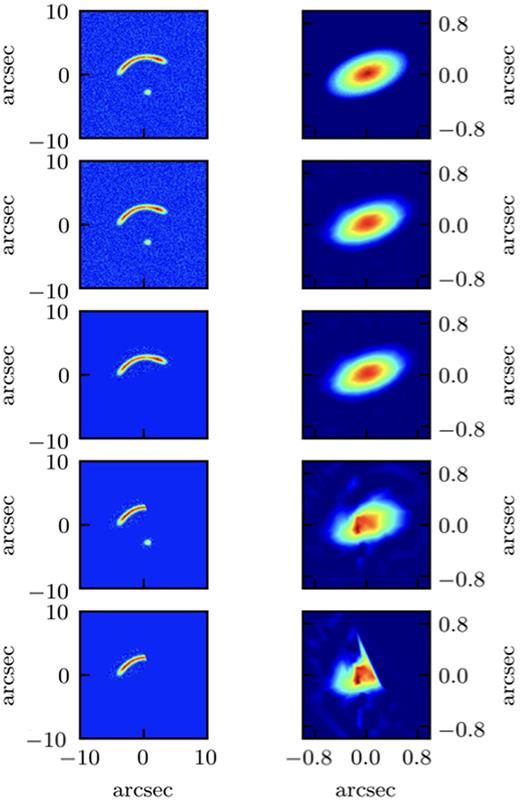
First row: on the left side the input lensed data obtained by lensing forward the disc galaxy on the right side. From second to fifth rows: reconstruction of the source (right-hand panels) obtained by modelling different parts of the mock lensed data (left-hand panels). Second row: all data are considered for the source reconstruction. Third row: the counter image is excluded. Fourth row: the counter image and only part of the arc are modelled. Fifth row: only part of the arc is modelled to reconstruct the source.

Open in new tab Download slide

6 SUMMARY AND CONCLUSION

In this paper, we have presented a new method to model the kinematics of strong gravitationally lensed galaxies from 3D emission-line observations. The technique is entirely Bayesian: a Bayesian penalty function allows us to simultaneously infer the lens–mass and the source–kinematic properties from the same 3D data cube, while the Bayesian marginalized evidence enables us to rank and compare different lens and kinematic models. This new approach is also grid-based and hierarchical. The source is reconstructed on a magnification-dependent Delaunay tessellation, and its kinematics represent the hyper-parameter of the source prior. The primary focus of this method is to provide a robust approach for studying the resolved kinematic properties of high-redshift lensed galaxies. In this respect, it represents a significant improvement over past and recent approaches. Indeed, since the kinematic model is a hyper-parameter of the reconstructed source, the inferred kinematic properties are not influenced by the poor understanding of the errors and spatial resolution on the unlensed plane. Furthermore, the lens–mass distribution is derived consistently from the same 3D data cube.

To test the capabilities of this new method in inferring the correct model parameters, we have studied a sample of nine simulated lensed galaxies as they would be observed with the OSIRIS spectrograph. These galaxies are characterized by a variety of rotation curves and geometries. In particular, we have focused on rotation curves that are described either by different functional forms (i.e. simulated data M1–M3) or derived from real galaxies (i.e. data sets M4–M6). We have found that this variety of shapes for the input rotation curves (from solid-body to flat rotation curves) is robustly recovered. In particular, the median relative accuracy on the inferred lens and kinematic parameters are at the level of ∼1 and ∼2 per cent, respectively.

Focussing on the extreme cases of a low-inclination (40°, M7) and edge-on (80°, M8) galaxy, we have also studied how the inclination of the source affects the accuracy of the reconstructions. We have found that the kinematic parameters can be recovered with a median accuracy of 1 and 2 per cent, respectively, if a reasonable initial estimate of the inclination can be obtained from the analysis of the zeroth-moment map. We have then tested the capability of our code to identify the presence of a warp. We have concluded that warps as large as 30 deg can significantly affect the lensed data. However, we are still able to recover the kinematic parameters with an accuracy of 3 per cent. The rotation curves in all cases are accurately reconstructed, therefore the most important physical parameters of the source galaxy (e.g. the dynamical mass, the angular momentum) can be correctly inferred.

We have also investigated the effect of increasing noise and concluded that the parameters are recovered with an accuracy better than 30 per cent whenever the SNR is higher than ∼3. The flat part of the rotation velocity is recovered with an accuracy of the order of 90 per cent even when the SNR is ∼3. Finally, we have examined the effect of strong radial motions and found it to be irrelevant for the typical angular and spectral resolution of IFU observations. From these extensive tests, we can conclude that the method presented in this paper offers a novel and robust way to study the gas kinematics of high-redshift lensed galaxies using data from the last generation of IFUs. Taking advantages of strong gravitational lensing, we can study the kinematic properties of galaxies at |$z$| ∼ 2–3 with spatial resolutions and SNR not achievable for unlensed galaxies, even with current observational technique. Moreover, gravitational lensing offers the unique opportunity to study galaxies in the low-stellar-mass range, which is almost impossible for studies targeting unlensed galaxies.

In this paper, we have focused on galaxy-scale lenses. The formalism of our method is also applicable to cluster lenses, although with a more complex parametrization of the lensing potential. However, as the mass distribution of galaxy clusters is more complicated, we expect in this case larger uncertainties on both the lens parameters and the source kinematics.

We have also only focused on optical observations. However, our technique, being an extension to the 3D domain of the methods developed by Vegetti & Koopmans (2009) and Rybak et al. (2015a), can also be used for the modelling of emission lines with radio interferometric observations. While our current implementation does not include functional forms for the analysis of radial motions and/or outflows, we plan to implement these in a follow-up work. In the near future, we will apply our novel technique to the analysis of both ionized and molecular gas emission lines to study the extended physical and kinematical properties of high-redshift lensed galaxies.

The code presented in this paper is not publicly available; however, the reader interested in using the code can contact the first author.

ACKNOWLEDGEMENTS

We thank an anonymous referee for a very careful report and for his/her comments. We thank Cristopher Fassnacht and Tucker Jones for their helpful comments and suggestions on the mock data. Simona Vegetti has received funding from the European Research Council (ERC) under the European Union’s Horizon 2020 research and innovation programme (grant agreement no. 758853). Enrico Di Teodoro acknowledges the support of the Australian Research Council through grant DP160100723.

Footnotes

1

The fitting of the input rotation curves for M3 to M6 was done using the Python package Scipy.optimize.

2

The median accuracies on |$\boldsymbol{\eta _{\mathrm{lens}}}$| and |$\boldsymbol{\eta _{\mathrm{kin}}}$| are calculated taking into account the relative difference between the input (Table 1) and recovered parameters (Table 3) as: (input-recovered)/input.

3

The values of the SNR are calculated as median of the SNR_i for each spectral channel i of the data cube. The latter is calculated as SNR|$_{\mathrm{i}}=\sum _{\mathrm{k}}S_{\mathrm{k i}}/\sqrt{N_{\mathrm{k i}}^2}$|⁠, where the sum is over the pixels of the |$\mathrm{i\text{}}$|th channel, S_ki is the signal at |$\mathrm{k\text{}}$|th pixel, and N_ki is its noise.

REFERENCES

Andersen

D. R.

,

Bershady

M. A.

,

Sparke

L. S.

,

Gallagher

J. S.

III,

Wilcots

E. M.

,

2001

,

ApJ

,

551

,

L131

10.1086/320018

Crossref

Search ADS

Blumenthal

G. R.

,

Faber

S. M.

,

Flores

R.

,

Primack

J. R.

,

1986

,

ApJ

,

301

,

27

Crossref

Search ADS

Bolton

A. S.

,

Burles

S.

,

Koopmans

L. V. E.

,

Treu

T.

,

Moustakas

L. A.

,

2006

,

ApJ

,

638

,

703

10.1086/498884

Crossref

Search ADS

Courteau

S.

,

1997

,

AJ

,

114

,

2402

10.1086/118656

Crossref

Search ADS

Courteau

S.

,

Dutton

A. A.

,

2015

,

ApJ

,

801

,

L20

10.1088/2041-8205/801/2/L20

Crossref

Search ADS

Cresci

G.

et al. ,

2009

,

ApJ

,

697

,

115

10.1088/0004-637X/697/1/115

Crossref

Search ADS

Di Teodoro

E. M.

et al. ,

2018

,

MNRAS

,

476

,

804

10.1093/mnras/sty175

Crossref

Search ADS

Di Teodoro

E. M.

,

Fraternali

F.

,

2015

,

MNRAS

,

451

,

3021

10.1093/mnras/stv1213

Crossref

Search ADS

Di Teodoro

E. M.

,

Fraternali

F.

,

Miller

S. H.

,

2016

,

A&A

,

594

,

A77

10.1051/0004-6361/201628315

Crossref

Search ADS

Dutton

A. A.

et al. ,

2011

,

MNRAS

,

416

,

322

10.1111/j.1365-2966.2011.19038.x

Crossref

Dye

S.

et al. ,

2015

,

MNRAS

,

452

,

2258

10.1093/mnras/stv1442

Crossref

Search ADS

Epinat

B.

,

Amram

P.

,

Balkowski

C.

,

Marcelin

M.

,

2010

,

MNRAS

,

401

,

2113

10.1111/j.1365-2966.2009.15688.x

Crossref

Search ADS

Feroz

F.

,

Hobson

M. P.

,

Bridges

M.

,

2009

,

MNRAS

,

398

,

1601

10.1111/j.1365-2966.2009.14548.x

Crossref

Search ADS

Feroz

F.

,

Hobson

M. P.

,

Cameron

E.

,

Pettitt

A. N.

,

2013

, preprint (arXiv:1306.2144)

Förster Schreiber

N. M.

et al. ,

2006

,

ApJ

,

645

,

1062

10.1086/504403

Crossref

Search ADS

Förster Schreiber

N. M.

et al. ,

2009

,

ApJ

,

706

,

1364

10.1088/0004-637X/706/2/1364

Crossref

Search ADS

Förster Schreiber

N. M.

et al., 2018, preprint (arXiv:1802.07276)

Freeman

K. C.

,

1970

,

ApJ

,

160

,

811

10.1086/150474

Crossref

Search ADS

Genzel

R.

et al. ,

2011

,

ApJ

,

733

,

101

10.1088/0004-637X/733/2/101

Crossref

Search ADS

Genzel

R.

et al. ,

2017

,

Nature

,

543

,

397

Girard

M.

et al. ,

2018

,

A&A

,

613

,

A72

10.1051/0004-6361/201731988

Crossref

Search ADS

Harrison

C. M.

et al. ,

2017

,

MNRAS

,

467

,

1965

10.1093/mnras/stx217

Crossref

Search ADS

Jones

T. A.

,

Swinbank

A. M.

,

Ellis

R. S.

,

Richard

J.

,

Stark

D. P.

,

2010a

,

MNRAS

,

404

,

1247

10.1111/j.1365-2966.2010.16378.x

Crossref

Jones

T.

,

Ellis

R.

,

Jullo

E.

,

Richard

J.

,

2010b

,

ApJ

,

725

,

L176

10.1088/2041-8205/725/2/L176

Crossref

Search ADS

Jones

T.

,

Ellis

R. S.

,

Richard

J.

,

Jullo

E.

,

2013

,

ApJ

,

765

,

48

10.1088/0004-637X/765/1/48

Crossref

Search ADS

Koopmans

L. V. E.

,

2005

,

MNRAS

,

363

,

1136

10.1111/j.1365-2966.2005.09523.x

Crossref

Search ADS

Krajnović

D.

,

Cappellari

M.

,

de Zeeuw

P. T.

,

Copin

Y.

,

2006

,

MNRAS

,

366

,

787

10.1111/j.1365-2966.2005.09902.x

Crossref

Search ADS

Lagattuta

D. J.

,

Vegetti

S.

,

Fassnacht

C. D.

,

Auger

M. W.

,

Koopmans

L. V. E.

,

McKean

J. P.

,

2012

,

MNRAS

,

424

,

2800

10.1111/j.1365-2966.2012.21406.x

Crossref

Search ADS

Lang

P.

et al. ,

2017

,

ApJ

,

840

,

92

10.3847/1538-4357/aa6d82

Crossref

Search ADS

Larkin

J.

et al. ,

2006

,

New Astron. Rev

,

50

,

362

10.1117/12.672061

Google Scholar

Crossref

Law

D. R.

,

Steidel

C. C.

,

Erb

D. K.

,

2006

,

AJ

,

131

,

70

10.1086/498683

Crossref

Search ADS

Law

D. R.

,

Steidel

C. C.

,

Erb

D. K.

,

Larkin

J. E.

,

Pettini

M.

,

Shapley

A. E.

,

Wright

S. A.

,

2009

,

ApJ

,

697

,

2057

10.1088/0004-637X/697/2/2057

Crossref

Search ADS

Leethochawalit

N.

,

Jones

T. A.

,

Ellis

R. S.

,

Stark

D. P.

,

Richard

J.

,

Zitrin

A.

,

Auger

M.

,

2016

,

ApJ

,

820

,

84

10.3847/0004-637X/820/2/84

Crossref

Search ADS

Lelli

F.

,

Verheijen

M.

,

Fraternali

F.

,

Sancisi

R.

,

2012

,

A&A

,

537

,

A72

10.1051/0004-6361/201117867

Crossref

Search ADS

Lelli

F.

,

McGaugh

S. S.

,

Schombert

J. M.

,

2016

,

AJ

,

152

,

157

10.3847/0004-6256/152/6/157

Crossref

Search ADS

Livermore

R. C.

et al. ,

2015

,

MNRAS

,

450

,

1812

10.1093/mnras/stv686

Crossref

Search ADS

Lovell

M. R.

, et al. ,

2018

,

MNRAS

,

481

,

1950

Crossref

Search ADS

Mason

C. A.

et al. ,

2017

,

ApJ

,

838

,

14

10.3847/1538-4357/aa60c4

Crossref

Search ADS

Mieda

E.

et al. ,

2014

,

PASP

,

126

,

250

10.1086/675784

Crossref

Search ADS

Miller

S. H.

,

Bundy

K.

,

Sullivan

M.

,

Ellis

R. S.

,

Treu

T.

,

2011

,

ApJ

,

741

,

115

10.1088/0004-637X/741/2/115

Crossref

Search ADS

Miller

S. H.

,

Ellis

R. S.

,

Sullivan

M.

,

Bundy

K.

,

Newman

A. B.

,

Treu

T.

,

2012

,

ApJ

,

753

,

74

10.1088/0004-637X/753/1/74

Crossref

Search ADS

Molina

J.

,

Ibar

E.

,

Swinbank

A. M.

,

Sobral

D.

,

Best

P. N.

,

Smail

I.

,

Escala

A.

,

Cirasuolo

M.

,

2017

,

MNRAS

,

466

,

892

10.1093/mnras/stw3120

Crossref

Search ADS

Nesvadba

N. P. H.

et al. ,

2006

,

ApJ

,

650

,

661

10.1086/507090

Crossref

Search ADS

Newman

S. F.

et al. ,

2013

,

ApJ

,

767

,

104

10.1088/0004-637X/767/2/104

Crossref

Search ADS

Patrício

V.

et al. ,

2018

,

MNRAS

,

477

,

18

10.1093/mnras/sty555

Crossref

Search ADS

Press

W. H.

,

Teukolsky

S. A.

,

Vetterling

W. T.

,

Flannery

B. P.

,

1992

,

Numerical Recipes in C. The Art of Scientific Computing

,

Cambridge Univ. Press

,

New York

.

Google Scholar

Google Preview

OpenURL Placeholder Text

WorldCat

Puech

M.

et al. ,

2008

,

A&A

,

484

,

173

10.1051/0004-6361:20079313

Crossref

Search ADS

Remus

R.-S.

,

Dolag

K.

,

Naab

T.

,

Burkert

A.

,

Hirschmann

M.

,

Hoffmann

T. L.

,

Johansson

P. H.

,

2017

,

MNRAS

,

464

,

3742

10.1093/mnras/stw2594

Crossref

Search ADS

Rix

H.-W.

,

Guhathakurta

P.

,

Colless

M.

,

Ing

K.

,

1997

,

MNRAS

,

285

,

779

10.1093/mnras/285.4.779

Crossref

Search ADS

Rogstad

D. H.

,

Lockhart

I. A.

,

Wright

M. C. H.

,

1974

,

ApJ

,

193

,

309

10.1086/153164

Crossref

Search ADS

Rubin

V. C.

,

Ford

W. K.

Jr.,

Thonnard

N.

,

1978

,

ApJ

,

225

,

L107

10.1086/182804

Crossref

Search ADS

Rybak

M.

,

McKean

J. P.

,

Vegetti

S.

,

Andreani

P.

,

White

S. D. M.

,

2015a

,

MNRAS

,

451

,

L40

10.1093/mnrasl/slv058

Crossref

Search ADS

Rybak

M.

,

Vegetti

S.

,

McKean

J. P.

,

Andreani

P.

,

White

S. D. M.

,

2015b

,

MNRAS

,

453

,

L26

10.1093/mnrasl/slv092

Crossref

Search ADS

Shirazi

M.

,

Vegetti

S.

,

Nesvadba

N.

,

Allam

S.

,

Brinchmann

J.

,

Tucker

D.

,

2014

,

MNRAS

,

440

,

2201

10.1093/mnras/stu316

Crossref

Search ADS

Skilling

J.

,

2004

, in

Fischer

R.

,

Preuss

R.

,

Toussaint

U. V.

, eds,

AIP Conf. Proc. Vol. 735, Bayesian Inference and Maximum Entropy Methods in Science and Engineering

.

Am. Inst. Phys

,

New York

, p.

395

10.1063/1.1835238

Google Scholar

Google Preview

OpenURL Placeholder Text

WorldCat

Crossref

Stark

D. P.

,

Swinbank

A. M.

,

Ellis

R. S.

,

Dye

S.

,

Smail

I. R.

,

Richard

J.

,

2008

,

Nature

,

455

,

775

Straatman

C. M. S.

et al. ,

2017

,

ApJ

,

839

,

57

10.3847/1538-4357/aa643e

Crossref

Search ADS

Suyu

S. H.

,

Marshall

P. J.

,

Hobson

M. P.

,

Blandford

R. D.

,

2006

,

MNRAS

,

371

,

983

10.1111/j.1365-2966.2006.10733.x

Crossref

Search ADS

Swinbank

A. M.

et al. ,

2015

,

ApJ

,

806

,

L17

10.1088/2041-8205/806/1/L17

Crossref

Search ADS

Swinbank

A. M.

et al. ,

2017

,

MNRAS

,

467

,

3140

10.1093/mnras/stx201

Crossref

Swinbank

A. M.

,

Bower

R. G.

,

Smith

G. P.

,

Wilman

R. J.

,

Smail

I.

,

Ellis

R. S.

,

Morris

S. L.

,

Kneib

J.-P.

,

2007

,

MNRAS

,

376

,

479

10.1111/j.1365-2966.2007.11454.x

Crossref

Search ADS

Swinbank

A. M.

,

Sobral

D.

,

Smail

I.

,

Geach

J. E.

,

Best

P. N.

,

McCarthy

I. G.

,

Crain

R. A.

,

Theuns

T.

,

2012a

,

MNRAS

,

426

,

935

10.1111/j.1365-2966.2012.21774.x

Crossref

Search ADS

Swinbank

A. M.

,

Smail

I.

,

Sobral

D.

,

Theuns

T.

,

Best

P. N.

,

Geach

J. E.

,

2012b

,

ApJ

,

760

,

130

10.1088/0004-637X/760/2/130

Crossref

Search ADS

Teklu

A. F.

,

Remus

R.-S.

,

Dolag

K.

,

Arth

A.

,

Burkert

A.

,

Obreja

A.

,

Schulze

F.

,

2018

,

ApJ

,

854

,

L28

10.3847/2041-8213/aaaeb4

Crossref

Search ADS

Tiley

A. L.

et al. ,

2016

,

MNRAS

,

460

,

103

10.1093/mnras/stw936

Crossref

Search ADS

Trachternach

C.

,

de Blok

W. J. G.

,

Walter

F.

,

Brinks

E.

,

Kennicutt

R. C.

Jr,

2008

,

AJ

,

136

,

2720

10.1088/0004-6256/136/6/2720

Crossref

Search ADS

Tully

R. B.

,

Fisher

J. R.

,

1977

,

A&A

,

54

,

661

Turner

O. J.

,

Harrison

C. M.

,

Cirasuolo

M.

,

McLure

R. J.

,

Dunlop

J.

,

Swinbank

A. M.

,

Tiley

A. L.

,

2017

, preprint (arXiv:1711.03604)

Übler

H.

et al. ,

2017

,

ApJ

,

842

,

121

10.3847/1538-4357/aa7558

Crossref

Search ADS

van Albada

T. S.

,

Bahcall

J. N.

,

Begeman

K.

,

Sancisi

R.

,

1985

,

ApJ

,

295

,

305

10.1086/163375

Crossref

Search ADS

Vegetti

S.

,

Koopmans

L. V. E.

,

2009

,

MNRAS

,

392

,

945

10.1111/j.1365-2966.2008.14005.x

Crossref

Search ADS

Wisnioski

E.

et al. ,

2011

,

MNRAS

,

417

,

2601

10.1111/j.1365-2966.2011.19429.x

Crossref

Search ADS

Wisnioski

E.

et al. ,

2015

,

ApJ

,

799

,

209

10.1088/0004-637X/799/2/209

Crossref

Search ADS

Wright

S. A.

,

Larkin

J. E.

,

Law

D. R.

,

Steidel

C. C.

,

Shapley

A. E.

,

Erb

D. K.

,

2009

,

ApJ

,

699

,

421

10.1088/0004-637X/699/1/421

Crossref

Search ADS

Wu

X.

,

Gerhard

O.

,

Naab

T.

,

Oser

L.

,

Martinez-Valpuesta

I.

,

Hilz

M.

,

Churazov

E.

,

Lyskova

N.

,

2014

,

MNRAS

,

438

,

2701

10.1093/mnras/stt2415

Crossref

Search ADS

Yuan

T.

et al. ,

2017

,

ApJ

,

850

,

61

10.3847/1538-4357/aa951d

Crossref

Search ADS

Zolotov

A.

et al. ,

2015

,

MNRAS

,

450

,

2327

10.1093/mnras/stv740

Crossref

Search ADS

APPENDIX A: SNR

In Fig. A1, we show the SNR for the same spectral channels shown in Figs. 5 and B1–B8. For each spectral channel, the noise is added considering the procedure described in Section 3.2 and the exposure time listed in Table 1.

Figure A1.

SNR for M1–M9. The spectral channels are the same shown in Fig. 5 for M1 and B1–B8 for M2–M9.

Open in new tab Download slide

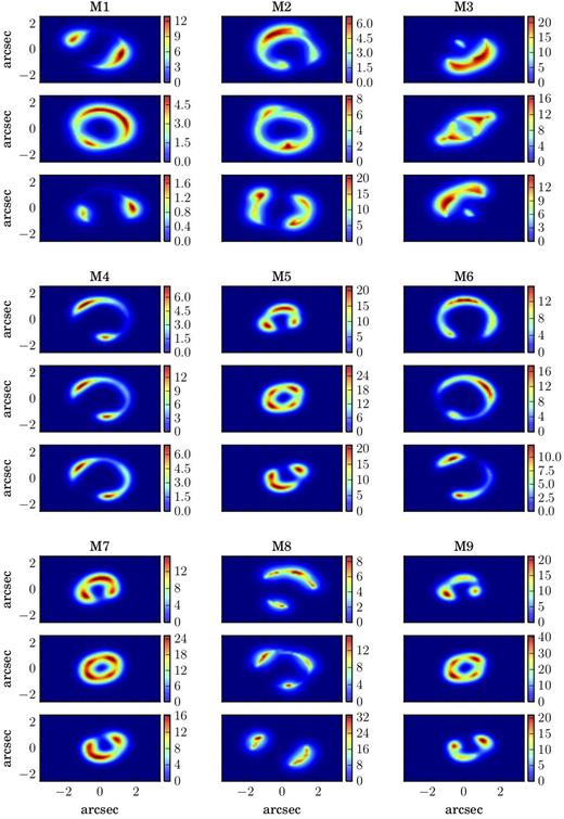
In Fig. A2, we show the SNR for the same spectral channels shown in Fig. 5 and for the different values of data quality, as described in Section 5.10 and summarized in Fig. 8. The six different noise levels are obtained by considering six values of the exposure times for M1: 14.4 ks, 7.2 ks, 3.6 ks, 1.8 ks, 900 s, and 600 s.

Figure A2.

SNR for the data-quality tests described in Section 5.10 and in Fig. 8. The different qualities of the data are obtained by using different exposure times, as indicated in the titles. The spectral channels are the same as shown in Fig. 5.

Open in new tab Download slide

APPENDIX B: MOCK data set M2–M9

As for Fig. 5 (for M1), we show in Figs. B1–B8 the input and best-fitting models for M2–M8. For a selected number of spectral channels, we plot in the first column the contour levels of the input source, in the second column the simulated lensed data, in the third column the inferred lensed model, in the fourth column the normalized image residuals, in the fifth column the reconstructed source, and in the sixth column the contour levels of the kinematic model.

Figure B1.

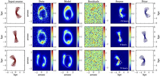
Same as Fig. 5 for the simulated data set M2, with n = {0.1, 0.2, 0.3, 0.4, 0.5, 0.6, 0.7, 0.8}.

Open in new tab Download slide

Figure B2.

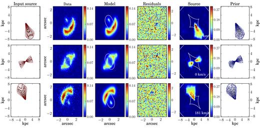
M3: same as Fig. 5 for the simulated data set M3, with n = {0.1, 0.2, 0.4, 0.6, 0.8}.

Open in new tab Download slide

Figure B3.

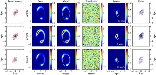
Same as Fig. 5 for the simulated data set M4, with n = {0.01, 0.05, 0.1, 0.2, 0.4, 0.6, 0.8}.

Open in new tab Download slide

Figure B4.

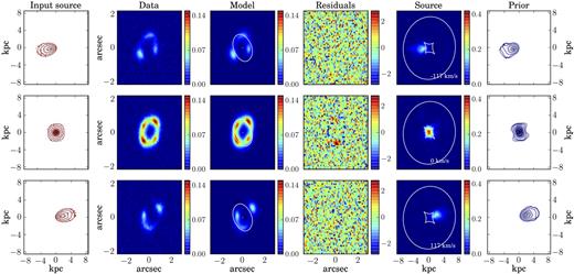
Same as Fig. 5 for the simulated data set M5, with n = {0.0250.05, 0.1, 0.2, 0.3, 0.4, 0.6, 0.8}.

Open in new tab Download slide

Figure B5.

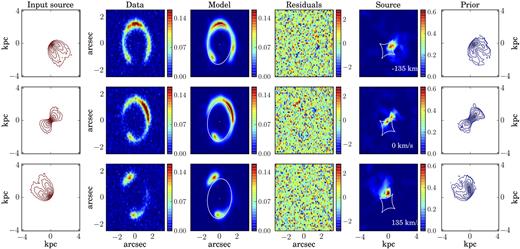
Same as Fig. 5 for the simulated data set M6, with n = {0.025, 0.05, 0.1, 0.2, 0.4, 0.6, 0.8}.

Open in new tab Download slide

Figure B6.

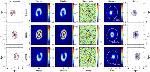
Same as Fig. 5 for the simulated data set M7, with n = {0.09, 0.18, 0.36, 0.54, 0.64, 0.72}.

Open in new tab Download slide

Figure B7.

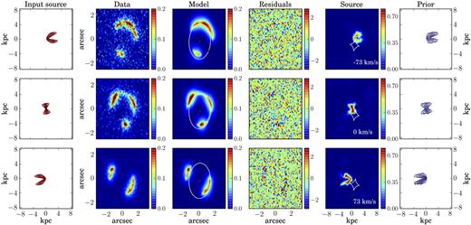
Same as Fig. 5 for the simulated data set M8, with n = {0.1, 0.2, 0.4, 0.6, 0.8}.

Open in new tab Download slide

Figure B8.

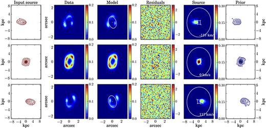
Same as Fig. 5 for the simulated data set M9, with n = {0.1, 0.2, 0.4, 0.6, 0.8}.

Open in new tab Download slide

This article is published and distributed under the terms of the Oxford University Press, Standard Journals Publication Model (https://dbpia.nl.go.kr/journals/pages/open_access/funder_policies/chorus/standard_publication_model)

Download all slides

Month:	Total Views:
September 2018	10
October 2018	22
November 2018	19
December 2018	11
January 2019	12
February 2019	7
March 2019	15
April 2019	7
May 2019	6
June 2019	11
July 2019	4
August 2019	3
September 2019	4
October 2019	23
November 2019	12
December 2019	6
January 2020	12
February 2020	4
March 2020	5
April 2020	5
June 2020	7
July 2020	7
August 2020	10
September 2020	8
October 2020	2
November 2020	2
December 2020	1
January 2021	2
February 2021	13
March 2021	8
May 2021	2
July 2021	3
September 2021	4
October 2021	2
November 2021	5
December 2021	18
January 2022	5
February 2022	7
March 2022	31
April 2022	15
May 2022	10
June 2022	14
July 2022	8
August 2022	16
September 2022	32
October 2022	10
November 2022	10
December 2022	18
January 2023	6
February 2023	19
March 2023	12
April 2023	8
May 2023	4
June 2023	7
July 2023	16
August 2023	14
September 2023	10
October 2023	9
November 2023	15
December 2023	24
January 2024	21
February 2024	25
March 2024	14
April 2024	23
May 2024	22
June 2024	34
July 2024	24
August 2024	12
September 2024	23
October 2024	18
November 2024	12
December 2024	2
January 2025	4
February 2025	16
March 2025	45
April 2025	24
May 2025	15

Article Contents

A novel 3D technique to study the kinematics of lensed galaxies Free

Abstract

1 INTRODUCTION

2 METHOD DESCRIPTION

2.1 Source reconstruction

2.1.1 First level of inference – linear optimization

2.1.2 Second level of inference – non-linear optimization

2.1.3 Third level of inference – model comparison

2.2 Lens–mass model

2.3 Source kinematic model

2.3.1 Rotation velocity and velocity dispersion curves

2.4 Optimization scheme

3 IFU MOCK DATA

3.1 Simulated sources

3.2 Simulated observations

4 MODELLING STRATEGY

4.1 Functional forms for the rotation velocity

5 RESULTS

5.1 Mock data set M1

5.2 Mock data set M2

5.3 Mock data set M3

5.4 Mock data set M4

5.5 Mock data set M5

5.6 Mock data set M6

5.7 Mock data set M7

5.8 Mock data set M8

5.9 Mock data set M9

5.10 Further tests

6 SUMMARY AND CONCLUSION

ACKNOWLEDGEMENTS

Footnotes

REFERENCES

APPENDIX A: SNR

APPENDIX B: MOCK data set M2–M9

Citations

Views

Altmetric

Email alerts

Astrophysics Data System

Citing articles via

Latest

Most Read

Most Cited

This Feature Is Available To Subscribers Only

A novel 3D technique to study the kinematics of lensed galaxies