


Abstract
We report the discovery of rapid variations of a high-velocity Mg ii broad absorption line (BAL) trough in the quasar SDSS J133356.02 + 001229.1 (|$z$|em ∼ 0.9197). Vivek et al. revealed the emergence and subsequent near disappearance of a BAL component in this source having an ejection velocity of ∼28 000 km s−1. Our further follow-up studies with South African Large Telescope (SALT) reveal the dramatic nature of the absorption line variability in this source. The absorption line emerged again at the same velocity and nearly disappeared within the SALT observations. Our observations allow us to probe variability over time-scales of the order of few days to 4.2 yr in the QSO rest frame. The observed velocity stability of BAL absorption does not point to any line-of-sight acceleration/deceleration of BAL clouds. The ionization parameter of the absorbing cloud is constrained from the column density ratio of Mg ii to Fe ii ground state absorption. In the absence of strong optical continuum variability, we suggest that photoionization-driven BAL variability due to changes in the shielding, multiple streaming clouds across our line of sight in a corotating wind, or a combination of both as possible explanations for the observed strong equivalent width variations.
1 INTRODUCTION
The radiative mode of active galactic nuclei (AGNs) feedback, operated through outflowing winds, has been proposed to be the most likely explanation for the observed supermassive black hole–host galaxy bulge coevolution and the star formation process (e.g. Di Matteo, Springel & Hernquist 2005; Higginbottom et al. 2013). The most direct evidence of disc winds in AGNs is provided by broad absorption line quasars (BALQSOs). These objects exhibit blue-shifted broad absorption lines, at least 2000 km s−1 wide, associated with strong resonance lines in the ultraviolet (UV) wavelengths. A vast majority of BALQSOs belong to the subclass called high ionization BAL (HiBAL) QSOs which only contain BALs of certain high ionization lines like N v, Si iv, and C iv. About 15 per cent of BALQSOs also show low ionization lines like Mg ii and Al iii together with the high ionization lines and are called low ionization BAL (LoBAL) QSOs. An even rarer population of BALQSOs (∼1 per cent) also contains broad absorption from excited fine-structure levels of iron which are known by FeLoBAL QSOs.
Absorption line variability studies of BALs are an important tool for understanding the gas dynamics occurring close to the central engine. Most of the previous variability studies of BALs mainly concentrated on high ionization lines like C iv and Si iv (Lundgren et al. 2007; Gibson et al. 2008; Capellupo et al. 2011; Filiz Ak et al. 2012, 2013; Vivek et al. 2014; Welling et al. 2014). This is partly due to the availability of a larger sample of HiBALs and partly due to the difficulty in disentangling the true BAL variability from Fe emission variability in LoBALs. Vivek et al. (2012b) probed the time variability of five FeLoBALs spanning an interval of up to 10 yr in the quasar rest frame and found strong variations of fine-structure Fe II UV 34 and UV 48 lines in the spectra of SDSS J221511.93-004549.9. Vivek et al. (2014) reported that LoBALs are found to be less variable compared to HiBALs in their spectroscopic monitoring study using 27 LoBALs. Although BALQSOs are known to vary in their absorption troughs, the most interesting cases of BAL variation are when the trough variability (1) exhibits signatures of radiative acceleration (for e.g. Srianand et al. 2002; Grier et al. 2016) or (2) is driven by photoionization (for e.g. Wang et al. 2015). Equally interesting are the cases where the BAL completely disappears or appears between two observations. There has been a handful of individual studies reporting disappearance/appearance of C iv BAL transients (Ma 2002; Hamann et al. 2008; Leighly et al. 2009; Krongold, Binette & Hernández-Ibarra 2010; Rodríguez Hidalgo, Hamann & Hall 2011). Filiz Ak et al. (2012) reported 19 cases of BAL trough disappearance in 21 sources in their studies using Baryon Oscillation Spectroscopic Survey (BOSS, Dawson et al. 2013) data. Vivek, Srianand & Gupta (2016) searched for transient BALs in a sample of 50 HiBALs and reported six cases of BAL appearance/disappearance. McGraw et al. (2017) found 14 disappearing BALs and 18 emerging BALs from their search of 470 quasars having multi-epoch observations in Sloan Digital Sky Survey (SDSS). All the previous studies attributed the BAL transience either to multiple streaming wind moving across the line of sight or to ionization-change scenario.
The first case of BAL transience in a LoBAL QSO was reported by Vivek et al. (2012a) in SDSS J133356.02 + 001229.1 (hereafter J1333 + 0012 at |$z$|em = 0.9197). In this previous study, Vivek et al. (2012a) identified two BAL components centred at ejection velocities of 17 000 km s−1 (R component) and 28 000 km s−1 (B component) in the SDSS spectra obtained in 2001. During our spectroscopic monitoring campaign using 2-m telescope at IUCAA Girawali Observatory (IGO) between 2008 and 2011, the R component completely disappeared whereas the B component emerged, strengthened in optical depth, widened in velocity, and nearly disappeared in 2011. In this paper, based on our continuous monitoring of this source, we study variability exhibited by this Mg ii BAL component over time-scales of the order of few days to 4.2 yr in the QSO rest frame. From 2008 onwards, this B component has shown dramatic variability between spectra obtained on any consecutive years. This article is organized as follows. In Section 2, we provide the details of our spectroscopic observations and data reduction. This section also provides some details of Catalina Real-Time Transient Survey (CRTS) data used to quantify the continuum variability of this quasar. In Section 3, we provide the statistical analysis of BAL variability. In Section 4, we discuss the observed variability in the frame work of different BALQSO models. Our results are summarized in Section 5.
2 OBSERVATION AND DATA REDUCTION
Our spectroscopic observations were primarily carried out with the IUCAA Faint Object Spectrograph (IFOSC) mounted on a 2-m telescope at IGO and the Robert Stobie Spectrograph (RSS, Kobulnicky et al. 2003; Smith et al. 2006) on South African Large Telescope (SALT). We also used two archival spectra available from the SDSS data release 12 (Alam et al. 2015). The details about the IGO observations and data reduction are given in Vivek et al. (2012a). Briefly, we used IFOSC to obtain high signal-to-noise spectra every year from 2008 to 2011 with R ∼ 1000 and wavelength coverage 3200–6800 Å. The two SDSS spectra obtained on 2001 and 2003 have R ∼ 2000 and a wavelength coverage of 3800–9200 Å.
We continued our monitoring campaign using RSS on SALT from 2012 to 2016. We used RSS in the long-slit mode with a 1.5 arcmin slit and the PG0900 grating. This combination gives a spectral resolution of 5 Å at a central wavelength of 5000 Å (R ∼ 1000) and a wavelength coverage of 3320–6440 Å. We also used the grating PG1300 once to obtain the spectrum with a different instrumental set-up. The seeing conditions were typically ∼2 arcsec for the observing runs. While a majority of the exposures had an integration time of 1200 s, there are four exposures with an integration time of 900 s and one exposure with an integration time of 2100 s. Within a single observing run, we also obtained multiple spectra separated by few days/weeks to probe the short time-scale variations. Data reduction was performed using standard IRAF1 scripts. The preliminary data reduction (gain correction, overscan bias subtraction, cross-talk-correction, and amplifier mosaicing) was done with the SALT reduction pipeline. Subsequently, we flat-fielded the data, applied a wavelength solution using arc lamp spectra, background subtracted the 2D spectra and extracted the 1D spectra around an aperture centred on the target. We also performed relative flux calibration on the data using standard stars. Absolute flux calibration was not performed due to the fixed nature of the SALT primary mirror and the strong variation in effective aperture with time and source position. In addition, there are also slit losses due to seeing being of the order of or bigger than the slit width which introduce further uncertainty in the flux scale. The details of the SALT observations are given in Table 1. As we did not find any detectable spectral variations between data obtained within a cycle (spanning ∼6 months), we combined the individual exposures obtained within a cycle.
Log of SALT observations.
| Name | Date | Grating | Cam-Angle | Exp. time | Airmass | Wavelength | Resolution | SNRa |
|---|---|---|---|---|---|---|---|---|
| (YYYY-MM-DD) | (deg) | (s) | (Å) | |||||
| 2012-05-09 | PG0900 | 25.75 | 1200 | 1.283 | 3320–6440 | 944 | 36.19 | |
| 2012-05-09 | PG0900 | 25.75 | 1200 | 1.254 | 3320–6440 | 944 | 42.40 | |
| 2012-05-31 | PG0900 | 25.75 | 1200 | 1.330 | 3320–6440 | 944 | 51.79 | |
| 2012-05-31 | PG0900 | 25.75 | 1200 | 1.399 | 3320–6440 | 944 | 50.64 | |
| 2012-06-01 | PG0900 | 26.5 | 1200 | 1.530 | 3460–6576 | 911 | 52.89 | |
| 2012-06-01 | PG0900 | 26.5 | 1200 | 1.270 | 3460–6576 | 911 | 56.84 | |
| 2012-06-03 | PG0900 | 25.75 | 1200 | 1.348 | 3320–6440 | 944 | 54.84 | |
| 2012-06-03 | PG0900 | 25.75 | 1200 | 1.205 | 3320–6440 | 944 | 56.93 | |
| 2013-05-01 | PG0900 | 25.75 | 1200 | 1.284 | 3320–6440 | 944 | 54.64 | |
| 2013-06-23 | PG0900 | 25.75 | 1200 | 1.293 | 3320–6440 | 944 | 41.14 | |
| 2013-06-23 | PG0900 | 25.75 | 1200 | 1.350 | 3320–6440 | 944 | 41.58 | |
| 2014-02-17 | PG0900 | 25.75 | 1300 | 1.269 | 3320–6440 | 944 | 9.56 | |
| 2014-02-17 | PG0900 | 25.75 | 1300 | 1.230 | 3320–6440 | 944 | 9.46 | |
| 2014-02-27 | PG0900 | 25.75 | 1000 | 1.334 | 3320–6440 | 944 | 50.25 | |
| 2014-03-13 | PG0900 | 25.75 | 1200 | 1.247 | 3320–6440 | 944 | 45.01 | |
| J133356.02 + 001229.1 | 2014-03-14 | PG0900 | 25.75 | 1009 | 1.188 | 3320–6440 | 944 | 28.84 |
| 2014-03-14 | PG0900 | 25.75 | 747 | 1.202 | 3320–6440 | 944 | 33.16 | |
| 2014-04-11 | PG0900 | 25.75 | 1300 | 1.234 | 3320–6440 | 944 | 52.69 | |
| 2014-04-11 | PG0900 | 25.75 | 1300 | 1.274 | 3320–6440 | 944 | 54.84 | |
| 2014-05-21 | PG0900 | 25.75 | 1300 | 1.221 | 3320–6440 | 944 | 55.32 | |
| 2014-05-21 | PG0900 | 25.75 | 1300 | 1.257 | 3320–6440 | 944 | 52.01 | |
| 2014-06-21 | PG0900 | 25.75 | 900 | 1.251 | 3320–6440 | 944 | 53.38 | |
| 2014-06-21 | PG0900 | 25.75 | 900 | 1.283 | 3320–6440 | 944 | 57.99 | |
| 2014-06-21 | PG0900 | 25.75 | 900 | 1.322 | 3320–6440 | 944 | 48.26 | |
| 2015-03-14 | PG1300 | 37.75 | 2100 | 1.193 | 3900–5990 | 824 | 53.35 | |
| 2015-04-20 | PG1300 | 37.75 | 1700 | 1.235 | 3900–5990 | 824 | 41.46 | |
| 2015-06-08 | PG0900 | 25.75 | 1700 | 1.207 | 3320–6440 | 944 | 64.05 | |
| 2016-02-11 | PG0900 | 25.75 | 1700 | 1.207 | 3320–6440 | 944 | 50.53 | |
| 2016-03-14 | PG0900 | 25.75 | 1700 | 1.207 | 3320–6440 | 944 | 56.94 | |
| 2016-04-13 | PG0900 | 25.75 | 1700 | 1.207 | 3320–6440 | 944 | 76.89 |
Note. a SNR per pixel estimated between the wavelength ranges 4500–4800 Å.
We obtained the continuum light-curve measurements for SDSS J1333 + 0012 from the Catalina Real-Time Transient Survey (CRTS, Drake et al. 2009). CRTS operates with an unfiltered set-up and the observed open magnitudes are transformed to V magnitudes using the equation, V = Vins + a(V) + b(V)*(B−V), where Vins is the observed open magnitude. The zero-point a(V) and slope b(V) are obtained from three or more comparison stars in the same field. On a given night, The CRTS obtains four such observations taken 10 min apart. Our spectroscopic observations have a good overlap with the CRTS observations.
3 BAL VARIABILITY: ANALYSIS & RESULTS
We first probed for short time-scale (13–65 d in the QSO frame) BAL variations in the SALT spectra of J1333 + 0012. Fig. 1 shows the short time-scale variations seen in the BAL components. Each panel shows the ratio spectra for each year obtained by taking the ratio of two spectra that have the maximum time separation between the observations for that year. The associated 3σ error on each ratio spectra are shown as red dotted lines. It is clear from this figure that there are no appreciable absorption line variations (i.e. more than 3σ level) on short time-scales. Hence, we combined all the individual spectra observed with the same observational set-up and obtained within one observing run i.e. spectra separated by a few days up to 3 months in the observed frame. We assign the average MJD as the MJD corresponding to the combined spectrum. This resulted in 10 high signal-to-noise spectra spanning the period 2008 to 2016. These spectra together with the two archival spectra available from the SDSS form the basis of our long time-scale (155 d–16 yr in quasar frame) BAL variability analysis presented in this paper.
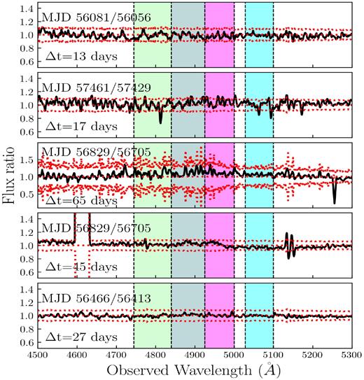
Short time-scale Mg ii absorption line variations in the SALT spectra of J1333 + 0012. Each panel shows the ratio spectra for each year obtained by taking the ratio of two spectra that have the maximum time separation between the observations for a given year. The associated 3σ error on each ratio spectra are shown as red dotted lines. The MJDs of the two observations and the time difference between the two in the QSO frame are marked in each panel.
We then fitted the continuum to all the spectra. The fitting procedure involves masking the wavelength range of bad pixels and BAL absorption (4644≤λ ≤5237 Å), and fitting the flux in the remaining pixels with a second order polynomial. In the case of BAL quasars, continuum measurements are difficult as the spectra are dominated by broad absorption. The narrow absorption lines seen in QSO spectra are found to be stable over long time-scales. J1333 + 0012 has two sets of narrow intervening absorption lines associated with two Mg ii systems at |$z$|abs = 0.8362 and 0.8984 on either sides of the BAL trough. We overcome the difficulty in continuum fitting by iterating the above continuum fitting procedure. The best continuum is chosen to be the one that produces minimum variations in the equivalent width of narrow intervening Mg ii absorption lines. The standard deviation of the equivalent width values of narrow Mg ii components for each best-fitting continuum procedure (0.277 Å) is taken to be the error associated with the continuum fitting procedure. We then normalized each epoch spectrum with the corresponding best-fitted continuum model.
Fig. 2 shows the comparison of continuum normalized spectra of all the epochs. As explained in Vivek et al. (2012b), we define two BAL components, namely ‘blue’ (hereafter, B component) and ‘red’ (hereafter, R component). The velocity limits of the B and R components were defined as the velocity after which the normalized flux rises above 0.9. The higher signal-to-noise ratio (SNR) SALT spectra allow us to further resolve the B component. The SALT spectrum obtained in the year 2015 showed the presence of three sub components. As our aim is to probe the BAL variations in different velocity sub-bins, we did not attempt to algorithmically define the velocity edges of the subcomponents. Rather, we divided the B component into three different components namely B1, B2, and B3 based on our visual inspection of the 2015 SALT spectrum. The R component originally detected in the early SDSS spectra never reappeared in our follow-up SALT observations. The wavelength regions of the three B components and the R component are shown in the figure by green-, grey-, blue-, and cyan-shaded regions. It is evident from Fig. 2 that all three B components show variations in the absorption strength between any consecutive year data. During our IGO monitoring campaign, the B component BAL absorption had a maximum strength in 2009 (i.e. MJD 54888) and nearly disappeared in 2011 (i.e. MJD 55657). We see the same trend of strengthening and fading for all the three components in our SALT monitoring campaign. The B components hit a maximum strength in 2014 (i.e. MJD 56829) and then nearly disappeared in our latest 2016 (i.e. MJD 57491) observations. McGraw et al. (2017) reported a fractional equivalent width change higher than 1.5 for the disappearing BAL troughs in their sample. In this study, we note that the BAL trough depths did not completely reach the continuum even in 2011 and 2016 when the trough depths were minimum. The fractional equivalent width changes in 2011 and 2016 are 1.0 and 1.2, respectively. Hence, we only claim a near disappearance rather than a complete disappearance for the B components. We notice that the B component variations happen over a time period of 3 yr in the observed frame. This correspond to a time-scale of 1.56 yr in the rest frame of the quasar.
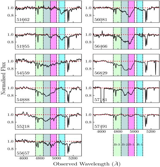
Comparison of continuum normalized spectra of all the epochs. The wavelength regions of the three B components and the R component are shaded in the figure by green, grey, blue, and cyan. In each panel, the number in the lower left denotes the average MJD corresponding to the spectrum.
We computed Mg ii equivalent widths for all four components in each spectrum. The wavelength regions used for the measurement and the resulting equivalent widths are listed in Table 2. We do measure non-zero equivalent width while integrating the transmitted flux over the red region. This could be related to the residual from the continuum fitting or due to a shallow absorption centred around 5150 Å unrelated to the red component seen in the SDSS spectrum. While we provide the measured equivalent width for this wavelength range, our focus in this paper is mainly on the blue component. The top panel of Fig. 3 shows the variation of Mg ii equivalent widths with MJD. The total as well as the individual equivalent width measurements for the identified regions of the blue Mg ii absorption line components clearly show the rapid variation observed within our observation campaign. We also computed the optical depth weighted velocity centroids, Vw, of Mg ii BAL absorption for all epochs. The middle panel shows the variation of optical depth weighted velocity centroid with MJD. We normalized the optical depth weighted velocity centroid of each absorption component by its mean velocity centroid (V(τ)) to compare the variation in different components. The optical depth weighted velocity centroids do not show large variations pointing to the velocity stability of BAL troughs. In the bottom panel of Fig. 3, we show the CRTS light curve. In the period over which the light curve is plotted, we see the quasar dimming a bit before brightening. However the maximum change is ∼0.3 mag. The light curve does not show any significant double peak seen in the equivalent width plot.
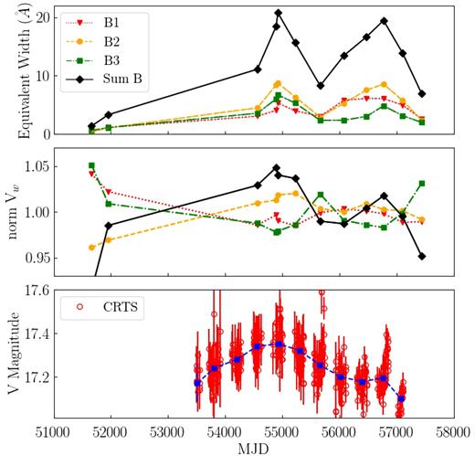
The top panel shows the variation of Mg ii equivalent widths with time for different BAL components. The middle panel shows the variation of normalized optical depth weighted velocity centroids, Vw, of different Mg ii BAL components. The bottom panel shows the variation of CRTS V-band magnitude over the same time. The blue dashed line in the bottom panel corresponds to the median magnitude averaged over 100 d.
Equivalent width measurements for the three BAL components.
| Instrument | MJDa | R Component | B1 Component | B2 Component | B3 Component | ||||
|---|---|---|---|---|---|---|---|---|---|
| centroid | W|$_R^{b}$| | centroid | W|$_{B1}^{c}$| | centroid | W|$_{B2}^{d}$| | centroid | W|$_{B3}^{e}$| | ||
| (× 103 km s−1) | (Å) | (× 103 km s−1) | (Å) | (× 103 km s−1) | (Å) | (× 103 km s−1) | (Å) | ||
| SDSS-2001 | 51662 | −17.29 ± 0.02 | 7.55 ± 0.44 | −25.07 ± 0.06 | 0.74 ± 0.46 | −26.89 ± 0.06 | 0.70 ± 0.49 | −36.09 ± 0.04 | 1.20 ± 0.50 |
| SDSS-2003 | 51955 | −17.47 ± 0.02 | 7.42 ± 0.37 | −24.61 ± 0.03 | 2.17 ± 0.38 | −27.12 ± 0.03 | 2.06 ± 0.39 | −34.64 ± 0.03 | 2.12 ± 0.40 |
| IGO-2008 | 54559 | −17.36 ± 0.03 | 3.66 ± 0.80 | −23.73 ± 0.02 | 5.87 ± 0.83 | −28.25 ± 0.02 | 8.61 ± 0.88 | −33.91 ± 0.02 | 6.84 ± 0.95 |
| IGO-2009 | 54888 | −16.28 ± 0.05 | 1.32 ± 0.43 | −23.99 ± 0.02 | 7.77 ± 0.43 | −28.35 ± 0.01 | 16.15 ± 0.43 | −33.58 ± 0.01 | 11.56 ± 0.45 |
| IGO 2009 | 54916 | −17.62 ± 0.03 | 2.68 ± 0.61 | −23.84 ± 0.01 | 10.22 ± 0.62 | −28.50 ± 0.01 | 16.82 ± 0.64 | −33.61 ± 0.01 | 12.89 ± 0.68 |
| IGO-2010 | 55218 | −16.73 ± 0.04 | 1.87 ± 0.38 | −23.71 ± 0.02 | 7.63 ± 0.38 | −28.54 ± 0.01 | 12.20 ± 0.38 | −33.86 ± 0.01 | 10.22 ± 0.39 |
| IGO-2011 | 55657 | −16.99 ± 0.03 | 3.09 ± 0.54 | −24.05 ± 0.02 | 5.82 ± 0.56 | −28.08 ± 0.02 | 5.58 ± 0.61 | −35.00 ± 0.02 | 4.50 ± 0.64 |
| SALT-2012 | 56081 | −16.93 ± 0.03 | 3.14 ± 0.29 | −24.15 ± 0.01 | 11.09 ± 0.29 | −27.98 ± 0.01 | 10.15 ± 0.29 | −34.02 ± 0.02 | 4.56 ± 0.29 |
| SALT-2013 | 56466 | −16.72 ± 0.04 | 1.49 ± 0.31 | −24.10 ± 0.01 | 11.73 ± 0.31 | −28.23 ± 0.01 | 14.47 ± 0.32 | −33.85 ± 0.02 | 5.79 ± 0.35 |
| SALT-2014 | 56829 | −16.95 ± 0.04 | 1.56 ± 0.29 | −24.02 ± 0.01 | 11.67 ± 0.29 | −28.05 ± 0.01 | 16.43 ± 0.30 | −33.75 ± 0.01 | 9.28 ± 0.30 |
| SALT-2015 | 57181 | −16.70 ± 0.03 | 1.40 ± 0.34 | −23.80 ± 0.01 | 9.54 ± 0.34 | −28.02 ± 0.01 | 11.08 ± 0.35 | −34.30 ± 0.01 | 6.06 ± 0.36 |
| SALT-2016 | 57491 | −16.36 ± 0.04 | 1.24 ± 0.30 | −23.82 ± 0.03 | 4.95 ± 0.30 | −27.75 ± 0.04 | 4.56 ± 0.31 | −35.41 ± 0.03 | 3.83 ± 0.31 |
Note.aMid-point of all the exposures taken in a year.
bComputed between 5028 and 5100 Å; while no absorption line similar to that seen in the SDSS spectrum reappeared anytime during our observations, we do measure non-zero equivalent widths probably due to continuum fitting residuals or from a shallow absorption centred around 5150 Å unrelated to the original red component.
cComputed between 4925 and 5000 Å.
dComputed between 4840 and 4925 Å.
eComputed between 4745 and 4840 Å.
Fig. 4 shows the variation of absolute fractional change in equivalent width, defined as |ΔW|/<W>, as a function of rest-frame time-lag for the blue absorption components. Each data point in Fig. 4 represents the median value of the absolute fractional change in equivalent widths binned by 500 rest-frame days. The lower and upper error bars correspond to the 25 and 75 percentile of the |ΔW|/<W> distribution within the bin. The dashed vertical lines mark the boundaries of the bins. Clearly, there is a difference in the amplitude of BAL variation between short time-scales (<1000 d) and long time-scales (>1500 d). Our spectra cover only the wavelength range of Fe ii lines associated with the broad Mg ii absorption. Neither in the individual spectrum nor in the combined spectrum, we detect Fe ii lines associated with the broad Mg ii absorption.
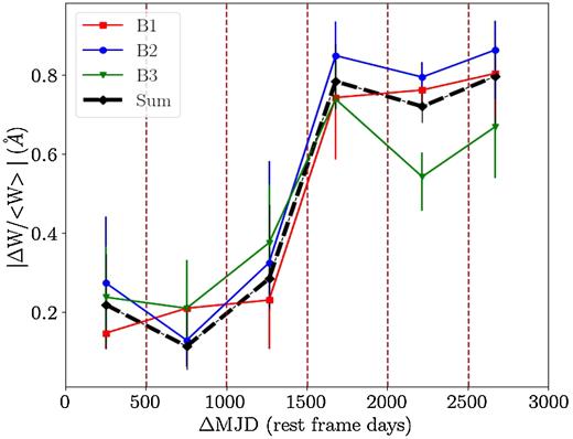
Median value of absolute fractional equivalent width variation of the blue Mg ii components binned in 500 d is plotted against the rest-frame time lags. The upper and lower error bars correspond to the 75 and 25 percentiles. The dashed vertical lines mark the boundaries of the time-lag bins.
3.1 Control sample of non-BALQSOs
The peculiar variations of J1333 + 0012 motivated us to construct a control sample of non-BALQSOs and to compare the various observational properties of J1333 + 0012 with that of the control sample QSOs. A control sample of 20 non-BALQSOs was identified from the SDSS DR7 QSO properties catalogue (Shen et al. 2011) using the k-nearest neighbour algorithm, which minimizes the distance in the redshift, absolute luminosity plane. Radio-loud quasars are often considered as a distinct group within the BALQSO sample. J1333 + 0012 has an integrated flux of 2.43 mJy at 1.4 Ghz in the FIRST catalogue. In terms of radio loudness parameter (Kellermann et al. 1989), J1333 + 0012 has a value of 3.35 and would not qualify as a radio-loud quasar. Following the procedure for the previous control sample, we also constructed another control sample containing only radio-quiet quasars. Fig. 5 shows the histogram distributions of the various QSO parameters for the objects in the two control samples. The dashed green and dotted red lines represent the median of the non-BAL and radio-quiet non-BAL distributions, respectively, and the blue star represents the parameter value for J1333 + 0012. The different panels represent the histogram distributions of redshift, absolute i-band magnitude, bolometric luminosity, FIRST integrated radio flux, equivalent width of Mg ii emission line, the power-law spectral index measured near the Mg ii emission line, full width at half-maximum (FWHM) of Mg ii emission line, black hole mass estimated from Mg ii emission line, and the resulting Eddington ratio. Except for the parameters in the third row, namely FWHM, black hole mass, and Eddington ratio, the parameter values for J1333 + 0012 are distributed around the median of the distribution for the two control samples. The distribution of parameters between the two control samples matches well with each other. We note that the FWHM of the Mg ii emission line in J1333 + 0012 is slightly higher compared to the FWHMs of Mg ii emission line in control sample QSOs. Black hole mass and Eddington ratio are derived from the Mg ii FWHM measurements. A control sample comprising of Mg ii BALs have larger dispersion in the redshift, and absolute i-band magnitude distributions as the fraction of LoBALs are much lower than HiBALs. With this caveat in mind, we note that the distribution of different parameters in the Mg ii BAL control sample matches well with the non-BAL control sample.
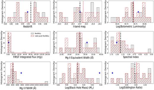
The histogram distributions of the various QSO parameters for the two control sample described in Section 3.1. The vertical and slanted hatched histograms represent the non-BAL and radio-quiet non-BAL control sample, respectively. The dashed green and dotted red lines represent the median of the non-BAL and radio-quiet non-BAL distributions, respectively. The blue star represents the parameter value for J1333 + 0012.
We used this control sample of 20 non-BALQSOs to generate a composite spectrum. To assemble the composite, we normalized each individual spectrum at 2500 Å and also distorted the spectral indices to have the same mean value. We also generated another composite from a control sample of QSOs selected from BOSS DR12 catalogue (Pâris et al. 2014). We find that the DR7 and DR12 composites are sufficiently similar to each other that we use the DR7 composite to compare with the J1333 + 0012 spectrum as we have access to other QSO properties from the (Shen et al. 2011) catalogue. Fig. 6 shows the comparison of J1333 + 0012 SDSS spectrum with the composite spectrum generated from the DR7 control sample QSOs (dashed/blue line). The Vanden Berk et al. (2001) composite is also shown as dotted/cyan line. Our composite spectrum generated from the DR7 control sample QSOs is similar to the Vanden Berk et al. (2001) non-BAL composite. Both the DR7 control sample composite and the Vanden Berk et al. (2001) non-BAL composite fail to fit the features red-wards of the Mg ii emission line. We then fit the J1333 + 0012 spectrum using three components: a power-law component, a double Gaussian component to fit the Mg ii emission line, and an Fe emission template from Vestergaard & Wilkes (2001). While fitting, we masked the wavelengths corresponding to the Mg ii BAL components (shaded region). The dot dashed/red line shows the Vestergaard & Wilkes (2001) Fe emission model fitting together with a power law and a double Gaussian. The Fe emission model better fits spectral features red-wards of the Mg ii emission line suggesting that J1333 + 0012 spectrum has significant contributions from iron emission. As has been previously noted, the Mg ii emission line of J1333 + 0012 appears to be slightly broader than the DR7 composite.
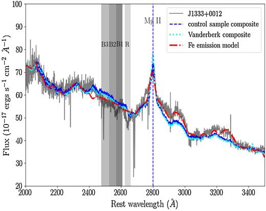
Comparison of J1333 + 0012 SDSS spectrum (solid grey) with the composite spectrum generated from the DR7 control sample (dashed/blue). The Vanden Berk et al. (2001) non-BAL composite is shown as dotted/cyan line. The dot dashed/red line shows the Vestergaard & Wilkes (2001) Fe emission model fitting together with a power law and double Gaussian.
4 DISCUSSION AND SUMMARY
The main result of our monitoring of J1333 + 0012 is that the three blue components of Mg ii absorption appear to vary in equivalent widths in phase over an extended period of time. Unlike the blue components, the red component, originally seen in the SDSS epochs, never reappeared during our spectroscopic monitoring campaign. In Vivek et al. (2012a), we explored the scenario where one lower velocity component (original red component) got accelerated to a higher velocity component (for details about acceleration scenario, see Section 4 of Vivek et al. 2012a). The reappearance of the blue components at the same velocities in the new SALT observations do not support the acceleration scenario.
It may be possible that we are observing J1333 + 0012 during a special time in its lifetime when it is trying to drive an outflow during its infancy. Evolutionary models for quasar outflows indeed have such a phase in the initial stages when the quasar is trying to blow off the dust and gas coccoon (for e.g. Boroson & Meyers 1992; Becker et al. 2000; Urrutia et al. 2009). Outflows facilitate the accretion on to the black hole by removing the angular momentum of the gas in the accretion disc. If the angular momentum removed by the outflow is equal to the angular momentum transferred from the accretion, one can obtain a linear relation between the outflow rate and the accretion rate (Konigl & Pudritz 2000). Episodic outflow ejections are reported in the case of young stellar objects (YSOs) that represent the earliest stages of stellar evolutions (for e.g. Bell & Lin 1994; Vorobyov & Basu 2005). Similarly, the appearing/reappearing outflows in J1333 + 0012 may be powered by episodic accretion events during the initial phases of quasar evolution. However, the reappearance of the BAL trough at the same velocity is less probable in the case of outflows powered by episodic accretion events. Hence, we do not favour the episodic outflow ejection model. Here, we explore various other scenarios that can explain the absorption line variability noted here.
4.1 Multiple streaming clouds across line of sight in a corotating wind
In the physical scenario of magnetocentrifugal driven winds (de Kool & Begelman 1995; Proga 2003; Everett 2005), winds corotate with the disc, at least close to the disc. Such a wind is made of dense clouds confined by the magnetic field, and therefore does not require shielding. Two of the predictions of this corotating wind scenario are high terminal velocities of the outflow and broader emission lines as compared to a non-rotating wind. We note that J1333 + 0012 has a maximum ejection velocity of 32 000 km s−1 while the average maximum ejection velocity in Vivek et al. (2014) is ∼5800 km s−1(see fig. 11 of Vivek et al. 2014). Thus, the velocity of J1333 + 0012 is on the higher side of the observed ejection velocities in BALQSOs. From Figs 5 and 6, we also note that the Mg ii emission line in J1333 + 0012 is broader than Mg ii emission lines in the control sample QSOs. The FWHM of the Mg ii emission line is 7552 km s−1 whereas the non-BALQSO, radio-quiet non-BALQSO, and LoBAL QSO control sample have a median value of 4000, 4100, and 4300 km s−1.
If the measured BAL radial velocity of 25 000 km s−1 is assumed to be close to the actual 3D velocity vector of the BAL cloud, a 1 × 10⁹ M⊙ blackhole indicates a Keplerian circular orbital period ∼2 yr. We note that Shen et al. (2011) report the blackhole mass for J1333 + 0012 as 6 × 10⁹ M⊙ and this blackhole mass estimate results in an orbital period of ∼10 yr. The maximum rest-frame time-scale probed by our observations is 4.2 yr. This would mean that the BAL cloud would have completed a significant fraction of a full rotation during our observations and the cloud would have moved out of the line of sight in 1–2 yr time-scale. In our observations, we do find that the BAL troughs nearly disappeared on a rest-frame time-scale of 2 yr. However, we do not favour the scenario where the same cloud reappearing again as the time-scale between near disappearance and subsequent reappearence is within a rest-frame year. The Keplerian circular orbit may be a too simple of an assumption given that the line of sight is very large. In reality, the cloud may be moving in an elongated elliptical orbit and the measured radial velocity may not be close to the true velocity of the BAL cloud. In an elongated elliptical orbit, if the cloud is moving in a direction close to the line of sight, the radial velocity will dominate over the transverse velocity. Vivek et al. (2012a) measured the transverse velocity of the BAL cloud to be 550 km s−1. The small value of transverse velocity as compared to the radial velocity would imply that the BAL cloud is indeed moving close to the line of sight in an elongated orbit.
When multiple clouds rotate with the disc, the distribution of clouds in the line of sight changes with time. In this scenario the strengthening and weakening of BAL absorption can be attributed to the covering fraction changes of the passing BAL clouds. The minimum of BAL absorption strength may be the case when the line of sight does not intersect any BAL cloud. Subsequent reappearance and evolution of BAL absorption may be attributed to the continued covering fraction changes of the BAL clouds. Although the reappearance of the second cloud at the same velocity seems less likely, it can happen if the clouds are density structures embedded in a bigger outflow.
4.2 Photoionization-driven BAL variability
Coordinated variations over large velocities may suggest that BAL variability is caused by changes in the ionization state of the absorbers. The photoionization induced variability can be well studied either when two or more absorption components from the same ion are detected or when there are absorption from different ions with similar ionization potential. As there is only a single Mg ii BAL component in our spectra, the only handle we have is to look for coordinated variations between continuum and absorption lines. However, previous studies on BAL variability have not detected any correlations between BAL absorption and continuum variations (Gibson et al. 2008; Filiz Ak et al. 2013; Vivek et al. 2014). If the density of the absorbing cloud is assumed to be constant, change in the ionization state of the gas can only happen with a change in the ionizing flux. Bottom panel of Fig. 3 shows the CRTS V-band light curve obtained roughly during the same time of our spectroscopic observations. The QSO continuum flux varied in concordance with the BAL variability during the first phase of BAL variability (i.e. between 2008 and 2011). When the BAL absorption got stronger, the QSO flux dimmed and vice versa. In Vivek et al. (2012a), we speculated this possible connection between QSO dimming and strengthening of Mg ii equivalent widths to some outflow ejection events in the accretion disc that cause reduction in the accretion efficiency. However, a similar concordant variability is not seen in the second phase of our monitoring (i.e. between 2012 and 2016).
We computed the limit on Fe ii line equivalent width corresponding to the velocity of the Mg ii blue component and then used CLOUDY v17.00 to model the photoionization properties of the absorbing cloud. CLOUDY is a spectral synthesis and plasma simulation code designed to simulate astrophysical environments (Ferland et al. 2017). We found the 3σ limit on the ground state Fe ii equivalent width to be 0.6 Å. Fe iii excited fine-structure line UV 49 is also covered in the SALT spectra. The 3σ limit for UV 49 line is found to be 1.5 Å. The left-hand panel in Fig. 7 shows the column densities of Mg ii (black/solid), ground state Fe ii(red/dashed), and ground state Fe iii (blue/dotted) lines as a function of ionization parameter. The right-hand panel shows the ratio of column densities of ground state Fe ii (black/solid) and ground state Fe iii (red/dashed) with respect to Mg ii column density. The black/dashed and red/dotted horizontal lines correspond to the lower limit on equivalent width ratios, W(Mg ii)/W(Fe ii) and W(Mg ii)/W(Fe iii) measured from the spectrum having strongest Mg ii absorption (obtained in the year 2014). In computing the above equivalent width ratios, we have used the total equivalent width of the Mg ii blue component rather than using the equivalent widths of the subcomponents. As none of the Mg ii lines are saturated, it is reasonable to approximate that the column densities and equivalent widths are linearly connected. Unfortunately, we do not detect Fe iii ground state transitions in any of our spectra. The current version of CLOUDY cannot handle Fe iii excited fine structure lines. So, we use the column densities of Mg ii and Fe ii for our calculations. The Mg ii to Fe ii column density ratio points to an ionization parameter range between −4 and −3. The right-hand panel of Fig. 7 shows that a small increase in ionization parameter around −3 can result in a large increase in the W(Mg ii)/W(Fe ii) ratio. This would mean that a large change in Mg ii column density without any Fe ii absorption can be achieved by a small change in the ionization parameter.
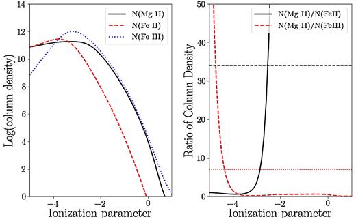
The left-hand panel shows the column densities of Mg ii (black/solid), ground state Fe ii (red, dashed), and ground state Fe iii (blue/dotted) lines as a function of ionization parameter. The right-hand panel shows the ratio of column densities of ground state Fe ii (black/solid) and ground state Fe iii(red/dashed) with respect to Mg ii column density. The dashed black line corresponds to the measured ratio of equivalent widths of Mg ii and Fe ii and dotted red line corresponds to the measured ratio of equivalent widths of Mg ii and Fe iii.
As our interest is in the long-term variations of the light curve, we employed a median filtering of the light curve with a window size of 200 d. The maximum and minimum magnitudes of the median filtered light curve is 17.09 and 17.35 mag. The QSO has only varied by ∼0.26 mag in the V-band light curve. This small change in magnitude alone cannot explain the observed large change in the Mg ii equivalent width (see fig. 2 of Hamann 1997). It is possible that the changes in the ionizing UV continuum is much more than the observed changes in the V band. In that scenario, photoionization changes in the BAL clouds due to the changes in the shielding gas can explain the observed variabilities in J1333 + 0012.
Radiation-driven wind models have postulated the existence of ‘hitchhiking/shielding gas’ which provides the shielding for the absorbing gas to prevent it from becoming over-ionized (Murray et al. 1995). The shielding gas is located between the continuum source and the outflowing gas. The ionizing flux impinging upon the outflow is the transmitted continuum through the shielding gas. In this model, variations in this shielding gas regulates the amount of ionizing continuum that reaches the absorbing gas (e.g. Arav et al. 2015), but does not necessarily affect the lower energy UV continuum. Variations in the shielding gas can be achieved either by a physical re-arrangement of the disc or by the corotation of shielding gas with the disc. Sim et al. (2010) did multidimensional hydrodynamical simulation of X-ray spectra for AGN accretion disc outflows and found out that the X-ray radiation scattered and reprocessed in the flow has an important role in determining the ionization conditions in the wind.
We used CLOUDY simulations to test the hypothesis of a high column density ‘shielding gas’ regulating the ionization conditions of the absorbing cloud. In this model, the shielding gas is located in between the continuum source and the BAL absorber. Recent line driven outflow simulations (Dyda & Proga 2018a, 2018) have predicted the existence of non-axisymmetric density features (clumps) at the base of the outflow. In the optically thick case, these clumps can affect the outflow by decreasing the available ionizing flux and altering the ionization state of the outflowing gas. The density of these clumps also differs by a factor of ∼3 from the azimuthal average. These clumps at the base of the outflow can be thought of playing the role of shielding gas. We ran two sets of photoionization simulations to test this hypothesis. In the first set of runs (hereafter, CLOUDY-I run) we used CLOUDY to obtain the continuum transmitted through the shielding gas. In the second set of runs (hereafter, CLOUDY-II run), we used the transmitted continuum from CLOUDY-I to study the photoionization conditions of the BAL cloud. In each of the CLOUDY-I run, we kept the flux of hydrogen-ionizing photons [log(ϕ(H)) = 12 cm−2 s−1] impinging the shielding gas cloud to be same and varied the total hydrogen column density of the shielding gas. This is equivalent to changing the shielding gas depth. We saved the transmitted continuum corresponding to the different values of the shielding gas column densities. We normalized each transmitted continua to the same monochromatic luminosity of 46.5 ergs s−1 at 0.1824 Ryd. This is to ensure that all the transmitted continua have the same power at a wavelength (beyond the main hydrogen absorption edge at 1 Ryd) that was not absorbed in the first set of CLOUDY runs. In CLOUDY-II runs, we used these normalized transmitted continua to determine the Mg ii column density of the BAL absorber at different distances from the shielding gas. For both CLOUDY-I and CLOUDY-II runs, we assumed a hydrogen density of nH = 1010cm∼s−3 that is similar to the hydrogen density in the broad line region. The left-hand panel of Fig. 8 shows the different transmitted continua for various values of shielding gas column densities. When the shielding gas column density increases above 1019 cm−2, significant amount of hydrogen ionizing photons are absorbed by the shielding gas. The middle and right-hand panel of Fig. 8 show the ratio of column densities of Mg ii to ground state Fe ii and Fe iii, respectively, as a function of the distance of the BAL absorber from the shielding gas. The red/dashed horizontal line in the middle and right-hand panels correspond to the measured upper limits on |$\frac{N(\rm{Mg\, {\small II}})}{N(\rm{Fe\, {\small II}})}$| and |$\frac{N(\rm{Mg\, {\small II}})}{N(\rm{Fe\, {\small III}})}$|. It is clear from Fig. 8 that the column density ratios of the BAL absorbing gas are sensitive to the column density of the shielding gas. We also ran these simulations for higher values of ϕ(H) when the number of hydrogen-ionizing photons is much higher than the hydrogen density of the shielding gas. In all our simulations, we find that when the BAL absorber distance is within a parsec from the shielding gas, the Mg ii column densities can change by several orders of magnitude for a narrow range of shielding gas hydrogen column density without producing significant Fe ii and Fe iii absorption. A factor of 15 change in equivalent width in the B component on SDSS J1333 + 0012 can be explained by a change of 1018 to 1019 cm s−2 in the column density of the shielding gas. The CLOUDY simulations reveal no significant change in the V-band flux due to this change in the shielding gas.
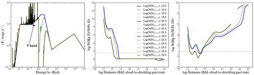
Left-hand panel: Transmitted continua for various values of shielding gas column density. The black arrow marks the location of the energy corresponding to the V-band central wavelength. Middle panel: Variation of the ratio of Mg ii to Fe ii column density as a function of distance between the BAL absorber and shielding gas for different values of hydrogen column density. Right-hand panel: Variation of the ratio of Mg ii to Fe iii column density as a function of distance between the BAL absorber and shielding gas for different values of hydrogen column density. The red/dashed horizontal line in the middle and right-hand panels corresponds to the observed upper limits on N(Mg ii)/N(Fe ii) and N(Mg ii)/N(Fe iii).
The changes in the shielding gas hydrogen column density can be achieved through Keplerian rotation. The BAL absorbers are typically thought to have a launching radii of ∼1000 Rs. The Keplerian orbital period of a cloud at this radius is 17 yr. As the location of shielding gas is in between the BAL absorber and the continuum source, the orbital period for the shielding gas will be even lesser. Thus, the shielding gas can have significant movement within our observed variability time-scale of 1–2 yr.
We do not see any appreciable changes in the strength of the Mg ii emission line between our observations. This would mean that the overall covering factor of the shielding gas is small. In Fig. 8, the energy corresponding to the redshifted V-band central wavelength is marked by the arrow. It is clear that the V-band continuum is not sensitive to the variations in the shielding gas.
While shielding gas scenario is a viable option for the variability of the blue absorption components, the same model will not explain the complete disappearance of the red component that did not reappear during our observations. This could either mean that the red and blue components are not colocated along our line of sight and have widely different physical conditions or more than one scenario is involved in the observed line variability. Further observations will shed more light on these issues.
CONCLUSION
In this paper, we report two cycles of appearance and near disappearance in the Mg ii broad absorption line outflow in SDSS J133356.02 + 001229.1. The blue component that appeared in 2001 is observed to first increase in absorption line strength in 2008. Reaching a maximum strength in 2009, it continued to decrease in strength and almost vanished in 2011. Furthermore, the absorption strength again started increasing in 2012, reached a maximum in 2014 and almost diminished in 2016.
Using CRTS light curves, we find that the quasar has not shown strong photometric variability that is correlated with the absorption line variability as expected in a simple photoionization scenario. However, these observations do not rule out a much larger variations in the ionizing continuum in the UV range. J1333 + 0012 has similar properties as that of a control sample of non-BALQSOs except for the FWHM of the Mg ii emission line. The Mg ii emission line FWHM of J1333 + 0012 is slightly higher as compared to the control sample.
Using photoionization simulations, we argue that the observed variations of the blue components can be explained by the variable photoionization conditions of the outflow regulated by the ‘shielding gas’ located at the base of the outflow. The V-band continuum is not sensitive to the changes introduced by the shielding gas. Photometric monitoring in the UV will allow us to test this scenario as the UV flux variations are expected to be larger than optical variations. No variation in the Mg ii emission line strength will be consistent with this scenario if the covering factor of the shielding gas is not very large. However, the variable shielding gas scenario cannot explain the disappearance of the red component that has never reappeared during our monitoring period. The observed absorption line variability can also be explained by multiple streaming gas moving across our line of sight. But, the reappearance of the second cloud at the same velocity seems less probable. It is more likely that the actual scenario may be a combination of variable shielding gas and multiple streaming gas. Continued monitoring of this source will be helpful to discern the actual nature of the outflow in J1333 + 0012.
ACKNOWLEDGEMENTS
The work of MV and KSD was supported in part by the U.S. Department of Energy, Office of Science, Office of High Energy Physics, under Award Number DE-SC0009959. The support and resources from the Center for High Performance Computing at the University of Utah are gratefully acknowledged. We thank the anonymous referee for a number of comments that helped us improve the paper.
Footnotes
IRAF is distributed by the National Optical Astronomy Observatories, which are operated by the Association of Universities for Research in Astronomy, Inc., under cooperative agreement with the National Science Foundation.
