


ABSTRACT
Statistical studies of galaxy–galaxy interactions often utilize net change in physical properties of progenitors as a function of the separation between their nuclei to trace both the strength and the observable time-scale of their interaction. In this study, we use two-point auto-, cross-, and mark-correlation functions to investigate the extent to which small-scale clustering properties of star-forming galaxies can be used to gain physical insight into galaxy–galaxy interactions between galaxies of similar optical brightness and stellar mass. The H α star formers, drawn from the highly spatially complete Galaxy And Mass Assembly (GAMA) survey, show an increase in clustering at small separations. Moreover, the clustering strength shows a strong dependence on optical brightness and stellar mass, where (1) the clustering amplitude of optically brighter galaxies at a given separation is larger than that of optically fainter systems, (2) the small-scale-clustering properties (e.g. the strength, the scale at which the signal relative to the fiducial power law plateaus) of star-forming galaxies appear to differ as a function of increasing optical brightness of galaxies. According to cross- and mark-correlation analyses, the former result is largely driven by the increased dust content in optically bright star-forming galaxies. The latter could be interpreted as evidence of a correlation between interaction-scale and optical brightness of galaxies, where physical evidence of interactions between optically bright star formers, likely hosted within relatively massive haloes, persists over larger separations than those between optically faint star formers.
1 INTRODUCTION
Historically, the field of galaxy interactions dates as far back as the 1940s; however, it was not until the 1970s that the concept of tidal forces being the underlying drivers of morphological distortions in galaxies was fully accepted. It was the pioneering works by Toomre & Toomre (1972) on numerically generating ‘galactic bridges and tails’ from galaxy interactions and by Larson & Tinsley (1978) on broad-band optical observations of discrepancies in ‘star formation rates (SFRs) in normal and peculiar galaxies’ that essentially solidified this concept. Since then, the progress that followed has revealed that interacting galaxies often show enhancements in H α emission (e.g. Keel et al. 1985; Kennicutt et al. 1987), infrared (IR) emission (e.g. Lonsdale, Persson & Matthews 1984; Soifer et al. 1984; Sanders et al. 1986; Solomon & Sage 1988), radio continuum emission (e.g. Condon et al. 1982), and molecular (CO) emission (e.g. Young et al. 1996) compared to isolated galaxies.
Over the past decade, numerous studies based on large-sky-survey data sets have provided ubiquitous evidence and signatures of tidal interactions. The enhancement of star formation is perhaps the most important and direct signature of a gravitational interaction (Kennicutt 1998; Wong et al. 2011); however, not all starbursts are interaction-driven, and not all interactions trigger starbursts. Starbursts, by definition, are short-lived intense periods of concentrated star formation confined within the galaxy and are expected to be triggered only by the increase in molecular gas surface density in the inner regions over a short time-scale. The tidal torques generated during the interactions of gas-rich galaxies are, therefore, one of the most efficient ways of funnelling gas to the centre of a galaxy (Di Matteo et al. 2007; Smith et al. 2007; Cox et al. 2008). In the absence of an interaction, however, bars of galaxies, which are prominent in spiral galaxies, can effectively facilitate both gas inflows and outflows (Regan & Teuben 2004; Owers et al. 2007; Ellison et al. 2011a; Martel, Kawata & Ellison 2013), and trigger starbursts. Nuclear starbursts appear to be a common occurrence of interactions and mergers; however, there are cases where starbursts have been observed to occur, for example, in the overlapping regions between two galaxies (e.g. the Antennae galaxies; Snijders, Kewley & van der Werf 2007).
In the local Universe, most interacting galaxies have been observed to have higher than average central star formation (e.g. Lambas et al. 2003; Smith et al. 2007; Ellison et al. 2008; Xu et al. 2010; Robotham et al. 2014; Scott & Kaviraj 2014; Knapen & Cisternas 2015), though in a handful of cases, depending on the nature of the progenitors, moderate (e.g. Rogers et al. 2009; Darg et al. 2010; Knapen & Cisternas 2015) to no enhancements (e.g. Bergvall, Laurikainen & Aalto 2003; Lambas et al. 2003) have also been reported. Likewise, interactions have been observed to impact circumnuclear gas-phase metallicities. In most cases, interactions appear to dilute nuclear gas-phase metallicities (e.g. Kewley et al. 2006b; Scudder et al. 2012; Ellison et al. 2013) and flatten metallicity gradients (e.g. Kewley, Geller & Barton 2006a; Ellison et al. 2008). There are also cases where an enhancement in central gas-phase metallicities (e.g. Barrera-Ballesteros et al. 2015) has also been observed. The other observational signatures of galaxy–galaxy interactions include enhancements in optical colours, with enhancements in bluer colours (e.g. De Propris et al. 2005; Darg et al. 2010; Patton et al. 2011) observed to be tied to gas-rich and redder colours to gas-poor interactions (e.g. Rogers et al. 2009; Darg et al. 2010), increased active galactic nucleus (AGN) activities (e.g., Rogers et al. 2009; Ellison et al. 2011b; Kaviraj et al. 2015; Sabater, Best & Heckman 2015), and substantially distorted galaxy morphologies (e.g. Casteels et al. 2013).
The strength and the duration of a physical change triggered in an interaction can potentially shed light on the nature of that interaction, progenitors, and the roles of their galaxy- and halo-scale environments in driving and sustaining that change. In this regard, the projected separation between galaxies, Rp, can essentially be used as a clock for dating an interaction, measuring either the time elapsed since or time to the pericentric passage.
One of the more widely used approaches to understanding the effects of galaxy–galaxy interactions involves directly quantifying net enhancement or decrement of a physical property as a function of Rp. For example, the strongest enhancements in SFR have typically been observed over <|$30\, h^{-1}_{70}$| kpc (e.g. Ellison et al. 2008; Li et al. 2008a; Wong et al. 2011; Scudder et al. 2012; Patton et al. 2013). The lower level enhancements, on the other hand, have been observed to persist for relatively longer time-scales. Ellison et al. (2008) report a net enhancement in SFR and a decrement in metallicity of ∼0.05–0.1 dex out to separations of ∼|$30\hbox{--}40\, h^{-1}_{70}$| kpc, and an enhancement in SFR out to wider separations for galaxy pairs of equal mass. Wong et al. (2011) report observations of SFR enhancements out to an ∼50 |$h_{70}^{-1}$| kpc based galaxy pair sample drawn from PRIMUS, Scudder et al. (2012) find that net changes in both SFR and metallicity persist out to at least |${\sim }80\, h^{-1}_{70}$| kpc, Patton et al. (2013) find a clear enhancement in SFR out to ∼150 kpc with no net enhancement beyond, Patton et al. (2011) report enhancement in colours out to ∼80 |$h_{70}^{-1}$| kpc, and Nikolic, Cullen & Alexander (2004) report an enhancement in SFR out to ∼300 kpc for their sample of actively star forming (SF) late-type galaxy pairs.
Even though the direct measure of a net change is advantageous as it can provide insight into dissipation rates and observable time-scales of interaction-driven alterations (Lotz et al. 2011; Robotham et al. 2014), as highlighted above, the reported values of Rp out to which a given change persists often varies. The strength and the scale out to which a physical change is observable are expected to be influenced by orbital parameters and properties of progenitors (Nikolic et al. 2004; Owers et al. 2007; Ellison et al. 2010; Patton et al. 2011), as well as by the differences in dynamical time-scales associated with short- and long-duration star formation events (Davies et al. 2015). Furthermore, galaxy–galaxy interactions do not always lead to observable changes. In particular, the subtle physical changes in Rp at which progenitors are just starting to experience the effects of an interaction can be too weak to be observed. A further caveat is that this method fails to provide any physical insights into potential causes for the observed changes, i.e. whether the change is a result of the first pericentric passage, second, or environment.
Another approach to studying the effects of galaxy–galaxy interactions involves two-point and higher order correlation statistics. The correlation statistics are often used in the interpretation of clustering properties of galaxies within one- and two-halo terms, and can be utilized with or without incorporating the physical information of galaxies. In this study, we aim to investigate whether a large-scale environment plays any role in driving and sustaining interaction-driven changes in SF galaxies with the aid of two-point correlation statistics.
In the local Universe, correlation functions have been ubiquitously used to study the clustering strength of galaxies with respect to galaxy properties like stellar mass, galaxy luminosities, and optical colours. Norberg et al. (2002) and Madgwick et al. (2003), for example, find clustering strength to be dependent strongly on galaxy luminosity. Zehavi et al. (2005b, 2011), Li et al. (2006, 2009), Ross et al. (2014), Favole et al. (2016), and Loh et al. (2010) report that galaxies with optically redder colours, which tend to be characterized with bulge-dominated morphologies and higher surface brightnesses, correlate stronger with the strength of clustering than those residing in the green valley or in the blue cloud.
Even though much work has been done in this area, very few of those studies have focussed on investigating the clustering of galaxies with respect to their SF properties such as SFR, specific SFR (sSFR), and dust. The Sloan Digital Sky Survey (SDSS) based analysis of Li et al. (2008a) reports a strong dependence of the amplitude of the correlation function on the sSFR of galaxies at Rp ≲ 100 kpc. They find a dependence between clustering amplitude and sSFR, where the amplitude is observed to increase smoothly with increasing sSFR such that galaxies with high specific SFRs are clustered more strongly than those with low specific SFRs. The strongest enhancements in amplitude are found to be associated with the lowest mass galaxies and over the smallest Rp. They interpret this behaviour as being due to tidal interactions. Using GALEX imaging data of SDSS galaxies, Heinis et al. (2009) investigate the clustering dependence on both (NUV − r) and sSFR. In the range |$0.01\lt R_{\rm p}\, (h^{-1}\, {\rm Mpc})\lt 10$|, they find a smooth transition in clustering strength from weak to strong as a function of the blue-to-red change in (NUV − r) and the low-to-high change in sSFR. It must be noted, however, that on the smallest scales the clustering of the bluest (NUV − r) galaxies shows an enhancement.
Coil et al. (2016) use the PRIMUS and DEEP2 galaxy surveys spanning the range 0.2 < |$z$| < 1.2 to measure the stellar mass and sSFR dependence of the clustering of galaxies. They find that clustering dependence is as strong a function of sSFR as of stellar mass, such that clustering smoothly increases with increasing stellar mass and decreasing sSFR, and find no significant dependence on stellar mass at a fixed sSFR. The same trend is also found within the quiescent population. The DEEP2 survey based study of Mostek et al. (2013) too finds that within the SF population the clustering amplitude increases as a function of increasing SFR and decreasing sSFR. Their analysis of small-scale clustering of both SF and quiescent populations, however, shows a clustering excess for high-sSFR galaxies, which they attribute to galaxy–galaxy interactions.
The spatial and redshift completenesses of a galaxy survey largely determine the smallest Rp that can be reliably probed by two-point correlation statistics, thus the ability to trace galaxy–galaxy interactions reliably. The lack of sufficient overlap between pointings to ensure the full coverage of all sources can significantly impact the spatial completeness of a fibre-based spectroscopic survey. The resulting spatial incompleteness can considerably decrease the clustering signal at Rp ≲ 0.2 Mpc, especially for non-projected statistics (Yoon et al. 2008), and can have non-negligible effects even on larger scales (Zehavi et al. 2005b). Therefore, many of the aforementioned studies are generally limited to probing clustering at Rp ≳ 0.1 h−1 Mpc .
For this study, we draw an SF sample of galaxies from the Galaxy And Mass Assembly (GAMA) survey (Driver et al. 2011; Liske et al. 2015), which has very high spatial and redshift completenesses (>98.5 per cent). GAMA achieves this very high spatial completeness by surveying the same field over and over (∼8–10 times) until all targets have been observed (Robotham et al. 2010, see the subsequent section for a discussion on the characteristics of the survey). Galaxy surveys like SDSS are limited both by the finite size of individual fibre heads and by the number of overlaps (∼1.3 times). Therefore, the GAMA survey is ideal for a study, such as ours, that investigates the small-scale-clustering properties of SF galaxies as a function of the SF properties.
This paper is structured as follows. In Section 2, we describe the characteristics of the GAMA survey and the different GAMA catalogues that have been used in this study. This section also details the spectroscopic completeness of the GAMA survey, the selection of a reliable SF galaxy sample from GAMA, and the construction of galaxy samples for the clustering analyses. The different clustering techniques and definitions used in this analyses, as well as the modelling of the selection function associated with random galaxies, are described in Section 3. Subsequently, in Section 4, we present the trends of SF galaxies with respect to different potential indicators of galaxy–galaxy interactions, and the correlation functions of SF based on auto-, cross-, and mark-correlation statistics. Finally, in Sections 5 and 6, we discuss and compare the results of this study with the results reported in other published studies of SF galaxies in the local Universe. This paper also includes four appendices, which are structured as follows. A discussion on sample selection and systematics is given in Appendix A. In Appendices B and C, we present a volume-limited analysis involving auto- and cross-correlation functions (ACFs and CCFs, respectively), and further correlation results involving different galaxy samples introduced in Section 2. Finally, in Appendix D, we present the mark-correlation analyses as we chose to show only the rank-ordered mark-correlation analysis in this paper.
The assumed cosmological parameters are H0 = 70 km s−1 Mpc−1, ΩM = 0.3, and |$\Omega _\Lambda =0.7$|. All magnitudes are presented in the AB system, and a Chabrier (2003) initial mass function (IMF) is assumed throughout.
2 GALAXY AND MASS ASSEMBLY (GAMA) SURVEY
We utilize the GAMA (Driver et al. 2011; Liske et al. 2015) survey data for the analysis presented in this paper. In the subsequent sections, we briefly describe the characteristics of the GAMA survey and the workings of the GAMA spectroscopic pipeline.
2.1 GAMA survey characteristics
2.1.1 GAMA imaging
GAMA is a comprehensive multiwavelength photometric and spectroscopic survey of the nearby Universe. GAMA brings together several independent imaging campaigns to provide a near-complete sampling of the ultraviolet (UV) to far-IR (0.15–500 |$\mu$|m) wavelength range, through 21 broad-band filters: FUV, NUV (GALEX; Martin et al. 2005), ugriz (Sloan Digital Sky Survey Data Release 7, i.e. SDSS DR7; Fukugita et al. 1996; Gunn et al. 1998; Abazajian et al. 2009), Z, Y, J, H, K (VIsta Kilo-degree INfrared Galaxy survey, i.e. VIKING; Edge et al. 2013), W1, W2, W3, W4 (Wide-field Infrared Survey Explorer, i.e. WISE; Wright et al. 2010), and 100 |$\mu$|m, 160 |$\mu$|m, 250 |$\mu$|m, 350 |$\mu$|m, and 500 |$\mu$|m (Herschel-ATLAS; Eales et al. 2010). A complete analysis of the multiwavelength successes of GAMA is presented at the end of the survey report of Liske et al. (2015) and in the panchromatic data release of Driver et al. (2015).
2.1.2 GAMA redshifts
GAMA’s independent spectroscopic campaign was primarily conducted with the 2dF/AAOmega multi-object instrument (Sharp et al. 2006) on the 3.9-m Anglo-Australian Telescope (AAT). Between 2008 and 2014, GAMA surveyed a total sky area of ∼286 deg2 split into five independent regions: three equatorial (called GAMA-09hr or G09, G12, and G15) and two southern (G02 and G23) fields of 12 × 5 deg2 each. The GAMA equatorial targets are drawn primarily from SDSS DR7 (Abazajian et al. 2009). We refer the readers to the paper by Baldry et al. (2010) for detailed discussions on target selection strategies and input catalogues. The equatorial fields have been surveyed to an extinction-corrected Petrosian r-band magnitude depth of 19.8. A key strength of GAMA is its high spatial completeness, in terms of both the overall completeness and completeness on small spatial scales. This is also advantageous for this study aimed at investigating SFR enhancement due to galaxy interactions via small-scale galaxy clustering. The tiling and observing strategies of the survey are discussed in detail in Robotham et al. (2010) and Driver et al. (2011). At the conclusion of the spectroscopic survey, GAMA has achieved a high-redshift completeness of 98.5 % for the equatorial regions, and we discuss in detail the spectroscopic completeness of the survey in Section 2.3.
2.1.3 GAMA spectroscopic pipeline
A detailed summary of the GAMA redshift assignment, re-assignment, and quality control procedure is given in Liske et al. (2015), according to which galaxy redshifts with normalized redshift qualities (NQ) ≥3 are secure redshifts. GAMA does not re-observe galaxies with high-quality spectra originating from other surveys, such that the GAMA spectroscopic catalogues comprise spectra from a number of other sources, e.g. SDSS, the 2-degree Field Galaxy Redshift Survey (2dFGRS; Colless et al. 2001), and the Millennium Galaxy Catalogue (MGC; Driver, Liske & Graham 2007) (see Section 2.3 for a discussion on the contribution of non-GAMA spectral measures to our analysis). Finally, given the exceptionally high redshift completeness of the GAMA equatorial fields, we restrict our analysis to the equatorial data.
The GAMA spectroscopic analysis procedure, including data reduction, flux calibration, and spectral line measurements, is presented in Hopkins et al. (2013). The GAMA emission line catalogue (SpecLineSFR) provides line fluxes and equivalent width (EW) measurements for all strong emission line measurements. A more detailed description of the spectral line measurement procedure and SpecLineSFR catalogue, in general, can be found in Gordon et al. (2017). Additionally, the strength of the λ4000-Å break (D4000) is measured over the D4000 bandpasses (i.e. 3850–3950 Å and 4000–4100 Å) defined in Balogh et al. (1999) following the method of Cardiel, Gorgas & Aragon-Salamanca (1998). SpecLineSFR also provides a continuum (6383–6538 Å) signal-to-noise ratio per pixel measurement, which is representative of the red end of the spectrum.
2.2 Galaxy properties
The two main intrinsic galaxy properties used in this investigation are H α SFRs and galaxy stellar masses. Below, we briefly overview the derivation of these properties and discuss their uncertainties.
2.2.1 H α star formation rates
The GAMA intrinsic H α SFRs are derived following the prescription of Hopkins et al. (2003), using the Balmer emission-line fluxes provided in SpecLineSFR. The spectroscopic redshifts used in the calculation are corrected for the effects of local and large-scale flows using the parametric multi-attractor model of Tonry et al. (2000), as described in Baldry et al. (2012), and the application of stellar absorption, dust obscuration, and fibre aperture corrections to SFRs is described in detail in Gunawardhana et al. (2013).
The luminosity-dependent (or SFR-dependent) dust obscuration, reflecting that massive SF galaxies also contain large amounts of dust relative to their low-SFR counterparts, is observationally well established in the local Universe (e.g. Hopkins et al. 2003; Brinchmann et al. 2004; Garn & Best 2010; Ly et al. 2012; Zahid et al. 2013; Jimmy et al. 2016). The mean variation in Balmer decrement with aperture-corrected H α luminosity for our sample is shown as blue points in Fig. 1, with red contours indicating the dependence of Balmer decrement on specific SFR. The dot–dashed line denotes the Balmer decrement approximately corresponding to the assumption of an extinction of 1 magnitude at the wavelength of H α for all galaxy luminosities (Kennicutt 1992). In this study, for galaxies without reliable Hβ flux measurements, we approximate a Balmer decrement based on the relation shown in blue in Fig. 1.
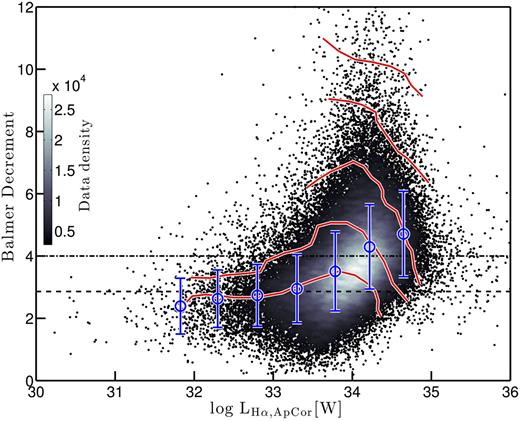
The distribution of Balmer decrement in aperture-corrected H α luminosity (|$L_{\rm {H}\alpha , \rm {ApCor}}$|, i.e. H α luminosity before correcting for dust obscuration) illustrating the luminosity dependence of dust obscuration. The grey colour scale shows the data density distribution of all SF galaxies. The black dashed and dot–dashed lines indicate the theoretical Case B recombination ratio of 2.86 and the Balmer decrement corresponding to the assumption of 1 mag extinction at the wavelength of H α. The blue points denote the mean variation and 1σ error in dust obscuration as a function of |$L_{\rm {H}\alpha , \rm {ApCor}}$|. The constant log sSFR contours, shown in red, are defined in steps of 0.3 dex, where log sSFR increases from −10.2 yr−1 at low Balmer decrements to −9 yr−1 at high Balmer decrements.
2.2.2 Stellar masses
The GAMA stellar masses and absolute magnitudes1 provided in the StellarMassesv16 (Taylor et al. 2011; Kelvin et al. 2012) catalogue are used for this study. A Bayesian approach is used in the derivation of the stellar masses, and are based on u, g, r, i, |$z$| spectral distributions and Bruzual & Charlot (2003) population synthesis models. Furthermore, the derivation assumes a Chabrier (2003) stellar IMF and Calzetti et al. (2000) dust law. The stellar mass uncertainties, modulo any uncertainties associated with stellar population synthesis models, are determined to be |${\sim }0.1\,$|dex. A detailed discussion on the estimation of GAMA stellar masses and the associated uncertainties can be found in Taylor et al. (2011).
2.3 Sample selection and spectroscopic completeness
We select a reference sample of galaxies, henceforth REF, consisting only of equatorial objects that satisfy both the GAMA main survey selection criteria (Baldry et al. 2010), and have spectroscopic redshifts, |$z$|spec, in the range 0.002 ≤ |$z$|spec < 0.35, representing the |$z$| window over which the H α spectral feature is observable in the GAMA spectra (Driver et al. 2011). The REF sample consists of 157 079 objects in total.
Out of the REF galaxies, those observed either as a part of GAMA and/or SDSS spectroscopic surveys with spectral signal-to-noise ratio > 3 form the spectroscopic sample. Objects with other survey spectra (e.g. 2dFGRS, MGC) are excluded as they lack the necessary information needed to reliably flux calibrate their spectra, and the objects with duplicate spectra2 are removed on the basis of their spectral signal-to-noise ratio, leaving 148 834 galaxies in the spectroscopic sample.
We assess the spectroscopic completeness of the survey by comparing the bivariate colour–magnitude distributions of REF and spectroscopic samples. Fig. 2(a) shows the colour–magnitude distribution of the ratio of spectroscopic-to-REF galaxies in a given r-band magnitude and apparent g − r colour, hereafter (g − r)app, cell, and the top and right-side panels show the completeness as a function of the r-band magnitude and (g − r)app. The exclusion of 2dFGRS spectra, in particular, leads to an overall incompleteness of ∼20 % across the three equatorial regions over the magnitude range probed by the 2dFGRS (green contours in Fig. 2(a) highlight the colour and magnitude range corresponding to the 2dFGRS galaxy distribution). The incompleteness present in each field, however, varies considerably, with G12 being the most incomplete (i.e. relatively a larger number of 2dFGRS galaxies reside in this region) and G09 being the most complete (i.e. no 2dFGRS galaxies reside in this region), as shown in the top panel of Fig. 2(a). Additionally, recall that GAMA spectral signal-to-noise ratio measures are representative of the red end of the spectrum; therefore, the application of a signal-to-noise ratio cut results in the incompleteness evident at fainter magnitudes and bluer colours in the same figure. The implication being that the spectroscopic sample is biased against optically faint bluer galaxies (the thin and thick black lines shown in the side panels of Fig. 2(a) clearly demonstrate this bias). Note that the variations in completeness seen at optically redder colours are largely driven by small number statistics. See Appendix A2 for a discussion on the impact of spectroscopic incompleteness on the results and conclusions of this study.
![(a) The apparent g − r colour, (g − r)app, and r-band Petrosian magnitude distributions of the ratios of spectroscopic-to-REF galaxies. The colour code corresponds to the percentage completeness with lighter colours indicating the deviation of the ratios from unity. The coloured contours show the approximate distfstar ribution of galaxies in our sample originating from the GAMA, SDSS, and 2dFGRS surveys. The top and side panels show completeness as a function of r-band Petrosian magnitude and (g − r)app, respectively, with black and thick grey lines showing the overall completeness across the three equatorial fields with (black) and without (grey) a spectral signal-to-noise ratio cut, and the coloured lines showing the completenesses for individual GAMA fields. (b) The (g − r)rest and Mr distribution of the ratio of SF-complete-to-REF galaxies. The closed contours from inwards to outwards enclose ∼25, 50, 75, and 90 % of the SF-complete data. Also shown are the constant mean log stellar mass ($\langle \log \mathcal {M}/\mathrm{M}_{\odot } \rangle$) and mean log SFR (〈log SFR [M$\odot$ yr−1]〉) contours corresponding to SF-complete galaxies. The top and side panels show the univariate Mr and (g − r)rest distributions of REF (black) and SF-complete (brown) galaxies, as well as the distribution all SF galaxies with reliably measured H α emission line fluxes (grey).](https://oup.silverchair-cdn.com/oup/backfile/Content_public/Journal/mnras/479/2/10.1093_mnras_sty1638/1/m_sty1638fig2.jpeg?Expires=1750475624&Signature=CXWS9WJNtHwO11pS~0nlfno1zWa9rGaBysv6yErtiM9PqbBH9kC2j3wOFrmtsoZ4mYTzvKCT-j~8xZJTTrgm8E61YZeBNMcQIdkRI8PgzBFjYLdcGrCZsrPuqsh9xBHqHVsFRRzw-iudQq6YhDEuP64huvvwBPsNTbO3g-L~yoPLi~6qHeZQXvv3-DlixyZWESYAkwFHK9CrTTX9nFpswKDIeRMH3VFeydcM9CdsyCGqempnTq7TkYnnwIn37jBaVQ2bCuHHJ3-uHJ6WlqkAn~9LOO3YU0x-Xul4wkpK9yLAnmLymtLEIe1yYEI4GV0LQYeTOAor6KwWttP3Qnx8Iw__&Key-Pair-Id=APKAIE5G5CRDK6RD3PGA)
(a) The apparent g − r colour, (g − r)app, and r-band Petrosian magnitude distributions of the ratios of spectroscopic-to-REF galaxies. The colour code corresponds to the percentage completeness with lighter colours indicating the deviation of the ratios from unity. The coloured contours show the approximate distfstar ribution of galaxies in our sample originating from the GAMA, SDSS, and 2dFGRS surveys. The top and side panels show completeness as a function of r-band Petrosian magnitude and (g − r)app, respectively, with black and thick grey lines showing the overall completeness across the three equatorial fields with (black) and without (grey) a spectral signal-to-noise ratio cut, and the coloured lines showing the completenesses for individual GAMA fields. (b) The (g − r)rest and Mr distribution of the ratio of SF-complete-to-REF galaxies. The closed contours from inwards to outwards enclose ∼25, 50, 75, and 90 % of the SF-complete data. Also shown are the constant mean log stellar mass (|$\langle \log \mathcal {M}/\mathrm{M}_{\odot } \rangle$|) and mean log SFR (〈log SFR [M|$\odot$| yr−1]〉) contours corresponding to SF-complete galaxies. The top and side panels show the univariate Mr and (g − r)rest distributions of REF (black) and SF-complete (brown) galaxies, as well as the distribution all SF galaxies with reliably measured H α emission line fluxes (grey).
Out of the galaxies with detected H α emission in the spectroscopic sample, those dominated by active galactic nucleus (AGN) emission are removed using the standard optical emission line ([N ii] λ6584/H α and [O iii] λ5007/Hβ) diagnostics (BPT; Baldwin, Phillips & Terlevich 1981) and the Kauffmann et al. (2003b) pure SF and AGN discrimination prescription. If all four emission lines needed for a BPT diagnostic are not detected for a given galaxy, then the two line diagnostics based on the Kauffmann et al. (2003b) method (e.g. log [N ii] λ6584/Hα > 0.2 and log [O iii] λ5007/Hβ > 1.0) are used for the classification. The galaxies that are unable to be classified this way are retained in our sample as a galaxy with measured H α flux but without an [N ii] λ6584 or [O iii] λ5007 measurement are more likely to be SF galaxies than AGNs (Cid Fernandes et al. 2011). Overall, ∼16 % of objects are classified either as an AGN or as an AGN–SF composite and are removed from the sample, and the ∼28 % unable to be classified are retained in the sample.
As a consequence of the bivariate magnitude and H α flux selection that is applied to our sample, our sample is biased against optically faint SF galaxies. This is a bias that not only affects any SF galaxy sample drawn from a broad-band magnitude survey, but it becomes progressively more significant with increasing |$z$| (Gunawardhana et al. 2015). Therefore, to select an approximately complete SF galaxy sample, henceforth SF complete, we impose an additional flux cut of 1 × 10⁻¹⁸ W m−2, which roughly corresponds to the turnover in the observed H α flux distribution of GAMA H α-detected galaxies (Gunawardhana et al. 2013).
A comparison between the SF-complete sample and REF galaxies in rest-frame g − r colour, hereafter (g − r)rest, and Mr space is shown in Fig. 2(b). The closed contours denote the fraction of the data enclosed, while the open black and grey contours denote constant 〈log SFR [M|$\odot$| yr−1]〉 and |$\langle \log \mathcal {M}/{\mathrm{M}_{{\odot }}} \rangle$| lines, respectively. Even though the SF-complete galaxies are dominated by optically bluer systems, a significant fraction of galaxies with optically redder colours have reliably measured H α SFRs, indicating ongoing star formation, albeit at lower rates. Also shown are the univariate Mr and (g − r)rest distributions of REF galaxies (black), SF-complete galaxies (brown), and of galaxies with reliable H α emission detections that are classified as SF following the removal of AGNs (grey) to illustrate how the H α flux cut of 1 × 10⁻¹⁸ W m−2 acts to largely exclude optically redder systems from our sample.
2.4 REF and SF-complete samples for clustering analysis
In order to investigate the clustering properties of SF galaxies with respect to optical luminosity and stellar mass (Sections 4.2–4.4), we use REF and SF-complete samples to further define three disjoint luminosity-selected, three disjoint stellar-mass-selected, and several volume-limited samples, for which all selection effects are carefully modelled.
The three disjoint luminosity-selected samples, called Mf, M*, and Mb, together cover the range −23.5 ≤ Mr < −19.5, and the three disjoint stellar-mass-selected samples, called |$\mathcal {M}_{\mathcal {L}}$|, |$\mathcal {M}_{\mathcal {I}}$|, and |$\mathcal {M}_{\mathcal {H}}$|, together span the range |$9.5\le \log \mathcal {M}$|/M|$\odot$| < 11. See Tables 1 and 2 for individual magnitude and stellar mass coverages of each luminosity- and stellar-mass-selected sample, as well as for a description of their key characteristics. We also define two redshift samples for each Mb, M*, and Mf, and for each |$\mathcal {M}_{\mathcal {H}}$|, |$\mathcal {M}_{\mathcal {I}}$|, and |$\mathcal {M}_{\mathcal {L}}$|, where one set covers the full redshift range of the SF-complete galaxies, and the second spans only the range 0.001 ≤ |$z$| ≤ 0.24.
The key characteristics of the three disjoint luminosity-selected subsamples (Mb: −23.5 ≤ Mr < −21.5; M*: −21.5 ≤ Mr < −20.5; Mf: −20.5 ≤ Mr < −19.5) drawn from the SF-complete and REF samples are given. For each sample, we provide the size of the sample, the average redshift and central ∼50% redshift range, median log sSFR [yr−1], (g − r)rest, and |$\log \, \mathcal {M}$| [M|$\odot$|] along with their central ∼50% ranges. We define two redshift samples for each Mb, M*, and Mf, where one sample covers the full redshift range over which the H α feature is visible in GAMA spectra (i.e. 0.001 < |$z$| < 0.34), and the second covers a narrower range 0.001 < |$z$| ≤ 0.24 (see Section 4.3). Using both the r-band magnitude selection of the GAMA survey and the H α flux selection of our sample, we estimate a completeness for each disjoint luminosity selected subsample, which is shown within brackets under Ngalaxies.
| Subset | Ngalaxies | 〈|$z$|〉 | |$z$| | log sSFR | log sSFR | 〈(g − r)rest〉 | (g − r)rest | 〈log |$\mathcal {M}\rangle$| | log |$\mathcal {M}$| |
|---|---|---|---|---|---|---|---|---|---|
| |$_{\sigma =25\%, 75\%}$| | [yr−1] | |$_{\sigma =25\%, 75\%}$| | |$_{\sigma =25\%, 75\%}$| | [M|$\odot$|] | |$_{\sigma =25\%, 75\%}$| | ||||
| SF complete | |||||||||
| Mb | 8100 (53%)a | 0.24 | (0.19, 0.29) | −10.28 | (−10.70, −9.87) | 0.55 | (0.47, 0.63) | 10.9 | (10.8, 11.1) |
| 3749 (68%) | 0.17 | (0.13, 0.21) | −10.67 | (−11.08, −10.13) | 0.60 | (0.51, 0.69) | 10.8 | (10.68, 10.99) | |
| M* | 20 976 (12%) | 0.21 | (0.18, 0.27) | −9.90 | (−10.20, −9.61) | 0.48 | (0.39, 0.56) | 10.46 | (10.31, 10.65) |
| 12 308 (62%) | 0.17 | (0.13, 0.21) | −10.11 | (−10.52, −9.79) | 0.50 | (0.41, 0.59) | 10.32 | (10.15, 10.50) | |
| Mf | 14 000 (<1%) | 0.14 | (0.11, 0.18) | −9.84 | (−10.14, −9.54) | 0.42 | (0.32, 0.51) | 9.98 | (9.81, 10.16) |
| 13 650 (<1%) | 0.14 | (0.11, 0.18) | −9.94 | (−10.24, −9.64) | 0.42 | (0.33, 0.51) | 9.83 | (9.66, 10.02) | |
| REF | |||||||||
| Mb | 33 406 | 0.25 | (0.20, 0.30) | – | – | 0.67 | (0.59, 0.75) | 10.95 | (10.83, 11.09) |
| M* | 64 618 | 0.22 | (0.18, 0.27) | – | – | 0.59 | (0.48, 0.72) | 10.50 | (10.34, 10.69) |
| Mf | 34 868 | 0.15 | (0.13, 0.19) | – | – | 0.51 | (0.37, 0.67) | 9.98 | (9.76, 10.20) |
aThe sample completeness.
The key characteristics of the three disjoint stellar-mass-selected subsamples (|$\mathcal {M}_{\mathcal {H}}$|: |$10.5\le \log \mathcal {M}/\mathrm{M}_{{\odot }}\le 11.0$|; |$\mathcal {M}_{\mathcal {I}}$|: |$10.0\le \log \mathcal {M}/\mathrm{M}_{\odot }\le 10.5$|; |$\mathcal {M}_{\mathcal {L}}$|: |$9.5\le \log \mathcal {M}/ \mathrm{M}_{\odot }\le 10.0$|) drawn from the SF-complete and REF samples are given. For each sample, we provide the size of the sample, average redshift and central ∼50% range, median log sSFR, (g − r)rest, and Mr along with their central ∼50% ranges. As described in the caption of Table 1, we define two redshift samples for each |$\mathcal {M}_{\mathcal {H}}$|, |$\mathcal {M}_{\mathcal {I}}$|, and |$\mathcal {M}_{\mathcal {L}}$|. The completeness of each sample due to the dual r-band magnitude and H α flux is indicated within brackets in the second column (after Ngalaxies), which is approximately the fraction of galaxies seen over the full volume. This value does not take into account the maximum volume out to which a galaxy of a given stellar mass would be detected.
| Subset | Ngalaxies | 〈|$z$|〉 | |$z$| | log sSFR | log sSFR | 〈(g − r)rest〉 | (g − r)rest | 〈Mr〉 | Mr |
|---|---|---|---|---|---|---|---|---|---|
| |$_{\sigma =25\%, 75\%}$| | [yr−1] | |$_{\sigma =25\%, 75\%}$| | |$_{\sigma =25\%, 75\%}$| | |$_{\sigma =25\%, 75\%}$| | |||||
| SF complete | |||||||||
| |$\mathcal {M}_{\mathcal {H}}$| | 11 600 (36%) | 0.23 | (0.18, 0.30) | −10.35 | (−10.72, −9.98) | 0.57 | (0.50, 0.64) | −21.53 | (−21.78, −21.29) |
| 5597 (61%) | 0.16 | (0.12, 0.21) | −10.57 | (−10.99, −10.17) | 0.61 | (0.54, 0.68) | −21.46 | (−21.72, −21.20) | |
| |$\mathcal {M}_{\mathcal {I}}$| | 18 103 (11%) | 0.20 | (0.14, 0.26) | −10.01 | (−10.29, −9.71) | 0.47 | (0.40, 0.54) | −20.82 | (−21.10, −20.55) |
| 12 135 (47%) | 0.16 | (0.12, 0.21) | −10.12 | (−10.43, −9.81) | 0.51 | (0.43, 0.58) | −20.69 | (−20.96, −20.43) | |
| |$\mathcal {M}_{\mathcal {L}}$| | 12 647 (<1%) | 0.15 | (0.11, 0.19) | −9.86 | (−10.16, −9.57) | 0.39 | (0.31, 0.45) | −20.01 | (−20.34, −19.69) |
| 11 648 (∼14%) | 0.14 | (0.10, 0.18) | −9.90 | (−10.18, −9.62) | 0.40 | (0.32, 0.46) | −19.95 | (−20.27, −19.66) | |
| REF | |||||||||
| |$\mathcal {M}_{\mathcal {H}}$| | 54 681 | 0.24 | (0.19, 0.29) | – | – | 0.67 | (0.60, 0.74) | −21.36 | (−21.61, −21.10) |
| |$\mathcal {M}_{\mathcal {I}}$| | 44 146 | 0.19 | (0.15, 0.24) | – | – | 0.55 | (0.44, 0.67) | −21.64 | (−20.95, −20.33) |
| |$\mathcal {M}_{\mathcal {L}}$| | 23 615 | 0.15 | (0.11, 0.18) | – | – | 0.42 | (0.33, 0.50) | −19.91 | (−20.26, −19.57) |
Out of the two redshift samples mentioned above, the former (i.e. the samples covering the full redshift range) is used for the autocorrelation analysis, and the latter for the cross- and mark-correlation analyses (Sections 4.3 and 4.4). The main reason for restricting the redshift coverage of galaxy samples in the latter case is to overcome the effects of the EW bias3 (Liang et al. 2004; Groves, Brinchmann & Walcher 2012; see also Appendix A). In this study, we find that the CCFs of low-sSFR galaxies spanning the range 0.24 ≤ |$z$| < 0.34 in redshift computed using two different clustering estimators, the Landy & Szalay (1993) and Hamilton (1993) estimators, differ systematically from each other, suggesting a failure in the modelling of the selection function of low-sSFR galaxies in the range 0.24 ≤ |$z$| < 0.34. The respective results for the low-sSFR galaxies in the range 0.01 ≤ |$z$| ≤ 0.24, on the other hand, are consistent with each other. Therefore, we limit the redshift range of all galaxy samples used for the cross- and mark-correlation analyses to 0.01 ≤ |$z$| ≤ 0.24.
The log sSFR and (g − r)rest distributions of the three disjoint luminosity-selected samples are shown in Figs 3 and 4. In Fig. 3, with increasing optical luminosity, the peak of the distribution of log sSFRs moves progressively towards lower sSFRs. The notably broader peak of the Mb distribution arises as a result of the bimodality present in the bivariate SFR (or sSFR) and |$\mathcal {M}$| distribution (see, for example, Fig. 10, shown later). Similarly, the (g − r)rest distributions show a progressive shift towards redder colours with increasing optical luminosity. From each disjoint luminosity-selected (stellar-mass-selected) sample, we select the 30 % highest and lowest sSFR (SFR), (g − r)rest, Balmer decrement, and D4000 (i.e. the strength of the 4000 Å break, Kauffmann et al. 2003a) galaxies to be used in the cross-correlation analysis (Section 4.3). The red and blue arrows in Figs 3 and 4 show these 30 % selections.
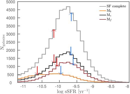
The log sSFR distributions of all SF-complete galaxies (grey), as well as Mb, M*, and Mf galaxies of the SF-complete sample. The redshift range considered is 0.001 < |$z$| ≤ 0.24, and the arrows indicate the sSFR cuts used to select the 30 % highest (blue arrows) and the 30 % lowest (red arrows) sSFR galaxies from each distribution.
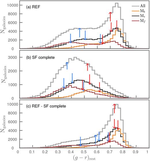
The (g − r)rest distributions of (a) all REF and (b) all SF-complete galaxies, as well as the distributions of their respective Mb, M*, and Mf subsamples. For completeness, we also show in panel (c) the distributions of REF–SF-complete galaxies. The redshift range considered is 0.001 < |$z$| ≤ 0.24, and the arrows indicate the colour cuts used to select the 30 % bluest (blue arrows) and the 30 % reddest (red arrows) colour galaxies from each distribution. The arrows show a clear change in position with luminosity (i.e. arrows move towards redder colours with increasing optical brightness), which is not seen with log sSFR (Fig. 3).
As none of the samples defined so far is truly volume limited, we define a series of volume-limited luminosity and stellar mass samples, which are described in Table B1. The volume-limited SF-complete samples are defined to be at least 95 % complete4 with respect to the bivariate r-band magnitude and H α flux selections. While this implies, by definition, that each volume-limited luminosity sample is at least 95 % volume limited, the same cannot be said about the volume-limited stellar mass samples. To achieve a 95 % completeness in volume-limited stellar mass samples would require the additional consideration of the detectability of a galaxy of a given stellar mass within the survey volume. It is, however, reasonable to assume that the ‘volume-limited stellar mass’ samples are close to 95 % volume limited, given the strong correlation between stellar mass and optical luminosity. For our sample, the 1σ scatter in stellar mass–luminosity correlation is ∼0.4 dex. The volume-limited REF samples have the same redshift coverage as their SF counterparts, and as such, they are 100 % complete with respect to their univariate magnitude selection.
3 CLUSTERING METHODS
In this section, we describe the modelling of the galaxy selection function using GAMA random galaxy catalogues, and introduce two-point galaxy correlation function estimators used in the analysis.
3.1 Modelling of the selection function
To model the selection function, we use the GAMA random galaxy catalogues (Random DMU) introduced in Farrow et al. (2015). Briefly, Farrow et al. (2015) employ the method of Cole (2011) to generate clones of observed galaxies, where the number of clones generated per galaxy is proportional to the ratio of the maximum volume out to which that galaxy is visible, given the magnitude constraints of the survey (Vmax, r), to the same volume weighted by the number density with redshift, taking into account targeting and redshift incompletenesses.
In effect, Random DMU provides Nr, with 〈Nr〉 ≈ 400, clones per GAMA galaxy in TilingCatv43. The clones share all intrinsic physical properties (e.g. SFR, stellar mass, etc.) as well as the unique galaxy identification (i.e. CATAID) of the parent GAMA galaxy, and are randomly distributed within the parent’s Vmax, r, while ensuring that the angular selection function of the clones matches that of GAMA. Therefore, for any galaxy sample drawn from TilingCatv43 based on galaxy intrinsic properties, an equivalent sample of randomly distributed clones can be selected from Random DMU by applying the same selection. If, however, a selection involves observed properties, then the clones need to be tagged with ‘observed’ properties before applying the same selection.
In order to select a sample of clones representative of galaxies in the SF-complete sample, first, we exclude the clones of GAMA galaxies not part of SF-complete sample. Secondly, each clone is assigned an ‘observed’ H α flux based on their redshift and their parent’s intrinsic H α luminosity. Finally, the clones with H α fluxes >|$1\times 10^{-18}\, {\rm W\, m}{^{-2}}$| and with redshifts outside the wavelength range dominated by the O2 atmospheric band but within the detection range of H α (i.e. SF-complete selection criteria) are selected for the analysis. The redshift distribution of the selected clones, hereafter random SF complete, normalized by the approximate number of replications (i.e. 〈Nr〉) is later shown in Fig. 6 (green line). Also shown for reference is the redshift distribution of the GAMA SF-complete sample (red line). The clear disagreement between the two distributions is a result of the differences in the selections. Recall that only the r-band selection of the survey is considered in the generation of clones, i.e. the clones are distributed within their parent’s Vmax, r, whereas we also impose an H α flux cut to select the SF-complete sample. In essence, we require the clones to be distributed within their parent’s min (Vmax, r, Vmax, Hα), where Vmax, Hα is the maximum volume, given the H α flux limit, in order to resolve the disagreement between the two distributions.
We show the mean variation of Nweight in SFR and Mr space in Fig. 5 for three different redshift bins. At a fixed Mr, Nweight declines with increasing SFR and redshift, and at a fixed SFR, Nweight decreases with increasing optical brightness and decreasing redshift. The implication being that the maximum volume out to which a high-SFR galaxy would be detectable is limited only by the r-band magnitude selection of the survey (i.e. no weighting is required), and vice versa. For example, a (low-SFR) galaxy with Nweight ≈ 20 has ∼20 clones out of ∼400 within its |$V_{\rm {max, \, H\alpha }}$|. While low-SFR galaxies can have larger values of Nweight, we demonstrate in Fig. 6 that the modelling of the redshift distribution is only very marginally affected by cutting the sample on Nweight. Moreover, in Appendix A, we show that the differences between the redshift distributions of clones weighted by Nweight with and without removing large values of Nweight are minimal. The differences are largely confined to lower redshifts, where most low-SFR systems reside. The impact of galaxies with large values of Nweight on the clustering results is, again, minimal, and is not surprising as most of the low-SFR systems with large Nweight lie outside the 90 % data contour (Fig. 5).
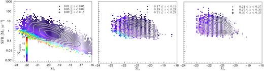
Mean weight applied to the random SF-complete sample as a function of their intrinsic SFR and Mr. The size of the markers indicates the mean redshift of GAMA SF-complete galaxies with a given SFR and Mr. The closed contours from inwards to outwards enclose 25, 50, 75, and 90 % of the data in the ranges 0.01 ≲ |$z$| < 0.15, 0.17 < |$z$| < 0.24, and 0.24 ≲ |$z$| < 0.35 (left- to right-hand panels). Only the lowest redshift sample (left-hand panel) contains galaxies with large Nweight measures.
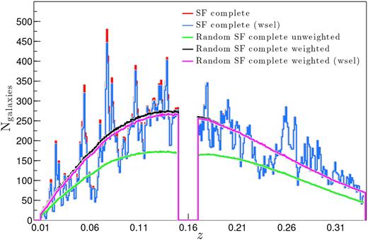
The redshift (0.01 ≲ |$z$| < 0.35) distribution of the SF-complete sample in comparison to the weighted (black and magenta lines) and non-weighted (green) distributions of the random SF-complete sample. The weights are determined according to equation (1), and the gap in the distributions centred around |$z$| ∼ 0.16 indicates the redshift range where the redshifted H α line overlaps with the atmospheric Oxygen-A band. The galaxies, both GAMA and random, with redshifts in this range are excluded from the analysis, as described in Section 2.3. Shown also are the weight-selected (wsel) distributions of the SF-complete sample and the equivalent weighted random SF-complete sample. These distributions exclude all galaxies (and their random clones) with Nweights > 10.
A comparison between the redshift distribution of the clones weighted by Nweight, called random SF complete weighted, and the distributions of the unweighted clones and GAMA SF galaxies is presented in Fig. 6. We also illustrate the relatively small effect on the weighted distribution if objects with Nweight > 10 (i.e. wsel selection in Fig. 6) are removed from the analysis. Consequently, the impact on the results of the correlation analyses is also minimal, as demonstrated in Appendix A1.
Alternatively, Nweight can also be calculated in redshift slices. We refer readers to Appendix A for a discussion on the resulting redshift distributions, mean Nweight variations with respect to SFR, Mr, and redshift, as well as on the clustering analysis. The main caveat in calculating Nweight in (smaller) redshift slices is that a relatively higher fraction of clones will require larger weights as Vzlim now defines the volume of a given redshift slice. For this reason, we choose to use Nweight calculated assuming a Vzlim defined by the detection limit of H α spectral line in GAMA spectra as described above for the clustering analysis presented in subsequent sections.
In summary, in this section, we presented a technique with which the available random clones of GAMA galaxies can be used, without the need to recompute them to take into account any additional constraints resulting from star formation selections.
3.2 Two-point galaxy correlation function
We integrate to |$\pi _{\rm {max}}\approx 40\, h^{-1}$| Mpc, which is determined to be large enough to include all the correlated pairs, and suppress the noise in the estimator (Skibba et al. 2009; Farrow et al. 2015).
There are several two-point galaxy correlation function estimators widely used in the literature (e.g. Peebles & Hauser 1974; Davis & Peebles 1983; Hamilton 1993; Landy & Szalay 1993). Here we adopt the Landy & Szalay (1993) estimator to perform the following: (i) two-point autocorrelation, (ii) two-point cross-correlation, and (iii) mark two-point cross-correlation analyses, as explained in the subsequent subsections. In Appendix A, we compare the results of Landy & Szalay (1993) with that obtained from the Hamilton (1993) estimator to check whether our results are in fact independent of the estimator used.
3.2.1 Two-point auto correlation function
The DD(rp, π), RR(rp, π), and DR(rp, π) are normalized data–data, random–random, and galaxy–random pair counts, and randoms are weighted by Nweight (equation 1).
3.2.2 Two-point cross correlation function
The D1D2(rp, π) is the normalized galaxy–galaxy pair count between data samples 1 and 2, and R1R2(rp, π) is the normalized random–random pair count between random clone samples 1 and 2, and the randoms are weighted by Nweight, as defined in equation (1).
The projected CCFs and their uncertainties are estimated following the same principles as the ACFs (Section 3.2.1).
3.2.3 Two-point mark-correlation function
Over the last few decades, numerous clustering studies based on auto- and cross-correlation techniques have quantitatively characterized the galaxy clustering dependence on galaxy properties in the low- to moderate-redshift Universe. While these studies use the physical information to define galaxy samples for auto- and cross-correlation analyses, that specific information is not considered in the analysis itself. In other words, galaxies are weighted as ‘ones’ or ‘zeros’, regardless of their physical properties, leading to a potential loss of valuable information. The mark clustering statistics, on the other hand, allow physical properties or ‘marks’ of galaxies to be used in the clustering estimation.
Again, we adopt the Landy & Szalay (1993) and Hamilton (1993) clustering estimators for this analysis.
4 SIGNATURES OF INTERACTION-DRIVEN STAR FORMATION
In this study, we consider several different physical properties of galaxies, such as sSFR, colour, dust obscuration, and the strength of the 4000 Å break (D4000), that are most likely to be altered in a galaxy–galaxy interaction. A discussion of these properties is given in Section 4.1, followed by the results of the auto- and cross-correlation analyses in Sections 4.2 and 4.3, respectively. Finally, in Section 4.4, we present the results of the mark-correlation analysis, where sSFRs and (g − r)rest of galaxies are used as marks to investigate the spatial correlations of SF galaxies.
4.1 Characteristics of GAMA star forming galaxies
The enhancement of star formation, or starburst, is perhaps the most important and direct signature of a gravitational interaction (Kennicutt 1998; Wong et al. 2011). There are several definitions of ‘starburst’ galaxies. Bolton et al. (2012), for example, define ‘starburst’ as SF galaxies with H α EWs, a proxy for sSFR, larger than 50 Å. Rodighiero et al. (2011), Luo, Yang & Zhang (2014), and Knapen & Cisternas (2015) use enhancement of SFR as a function of stellar mass to identify starbursts. Additionally, the evidence of certain ionized species (e.g. [Ne iii] λ3869 Å) indicative of the high ionization state of gas, as well as the overall enhancement of emission features in galaxy spectra (e.g. [O ii], [O iii], H α, Hβ), are other signatures of starbursts (Wild et al. 2014). Despite the differences, most ‘starburst’ definitions rely on spectral and/or physical properties of galaxies that are powerful tracers of SFR per unit mass.
The sSFR and |$\mathcal {M}$| distribution of SF galaxies used in this analysis (filled contours) is presented in Fig. 7. Overplotted are several well-known ‘starburst’ definitions in the literature; red open contours show the distribution of starbursts (H α EW >50 Å, Rodighiero et al. 2011), and the dotted and dashed dark pink lines denote the star formation main sequence (solid dark pink line, Elbaz et al. 2007) based on starburst definitions (e.g. Rodighiero et al. 2011; Silverman et al. 2015). The rest of the lines indicate the selection limits of the 30 % highest sSFR galaxies of Mb, M*, and Mf samples. Note that most of the galaxies selected based on the 30 % highest sSFR criterion are in fact those that qualify as starbursts according to the different starburst definitions discussed above.
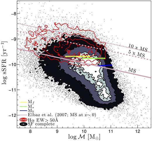
The sSFR and |$\mathcal {M}$| distribution of SF-complete galaxies. The filled-in and red contours enclose 25, 50, 75, and 94 % of SF-complete galaxies and SF-complete galaxies with H α EW >50 Å (i.e. the ‘starburst’ definition of Rodighiero et al. 2011), respectively. The dark pink lines denote the |$z$| ∼ 0 star formation main sequence (solid line, Elbaz et al. 2007), and two starburst selections, 5× (dashed line) and 10× the main sequence (dotted line), generally used in the literature (e.g. Rodighiero et al. 2011; Silverman et al. 2015). The rest of the lines (yellow, green, and blue) show the 30 % highest sSFR selections applied to the three disjoint luminosity-selected galaxy samples used in this analysis (see Table 1).
The signatures of interaction-driven star formation that we consider for this analysis are sSFR, SFR, colour, D4000, and Balmer decrements, and we use the BPT diagnostics to show (average) variations of these properties in SF galaxies (Figs 8 and 9). The BPT diagnostics themselves are indicators of gas-phase metallicities (i.e. oxygen abundances) in galaxies (Pettini & Pagel 2004) that can be heavily affected by pristine gas inflows and enriched gas outflows triggered during an interaction. Overall, relatively more massive and lower sSFR galaxies in our SF sample have higher metallicites (Fig. 8) and are characterized by redder optical colours and D4000 indices (Fig. 9)
![The mean variation in sSFR, SFR, and stellar mass (i.e. $\log \, \mathcal {M}$) of SF galaxies across the BPT plane in two redshift bins (from the top to bottom, with the key shown in the leftmost panels). The mean value of each property in a given [O iii]/Hβ and [N ii]/H α (i.e. the BPT diagnostics) bin is shown in colour, with the black line denoting the Kauffmann et al. (2003b) AGN/SF discrimination criterion. The contours enclose ∼25, 50, 75, and 90 % of the data in each redshift range.](https://oup.silverchair-cdn.com/oup/backfile/Content_public/Journal/mnras/479/2/10.1093_mnras_sty1638/1/m_sty1638fig8.jpeg?Expires=1750475624&Signature=ivJzsRemRYPR33OZVwNDWWxNhIOpwE~9t2DhqVsoGBBXTZkep7BgmvBKwlpk7uDlTw0mUH82ZT~FuZY6LCDCkQDOAeojvEWir8WUqgB919oPi59D2Bn6FLv2RUo1Yo~CBzUvbF2ESnuliFQyf0DUT8ZNBrNj40cQ6CkiVW-PAG-wGinXBnYOnGi8U2VL3CpZeeDWTNXaYUXMry8pXudlPX41XWd2~TyOabGhcKwWdMQoAm3A0BfrFO63boFjqLR99nqtTBd0gElEGfD~hS84K0U3ghODcglWkfu1HgvDl2wrevTvWFyDzIhTIr0uva~ngTyXgKwdPGnJxOc-aq26AA__&Key-Pair-Id=APKAIE5G5CRDK6RD3PGA)
The mean variation in sSFR, SFR, and stellar mass (i.e. |$\log \, \mathcal {M}$|) of SF galaxies across the BPT plane in two redshift bins (from the top to bottom, with the key shown in the leftmost panels). The mean value of each property in a given [O iii]/Hβ and [N ii]/H α (i.e. the BPT diagnostics) bin is shown in colour, with the black line denoting the Kauffmann et al. (2003b) AGN/SF discrimination criterion. The contours enclose ∼25, 50, 75, and 90 % of the data in each redshift range.
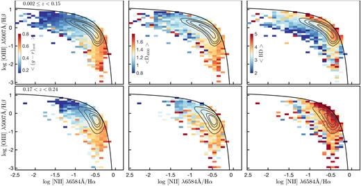
Same as Fig. 8, but now showing the mean variation of (g − r)rest, D4000, and Balmer decrement (i.e. BD) of SF galaxies across the BPT plane in two redshift bins.
Galaxy interactions impact dust to a lesser extent than metallicities as inflowing pristine gas cannot dilute the line-of-sight dust obscuration, though outflows can remove dust from the interstellar medium. The dust is thought to rapidly build up during a burst of star formation (da Cunha et al. 2010; Hjorth, Gall & Michałowski 2014), giving rise to the observed relationship between dust obscuration and host-galaxy SFR (Garn & Best 2010; Zahid et al. 2013). This relationship between dust obscuration and SFR is evident in Fig. 9 (right-hand panels), where the increment in Balmer decrement approximately mirrors the increase in SFR.
The observed bimodality in optical colours (Baldry et al. 2004) can also be used to assess the level of star formation in galaxies. A sudden influx of new stars alters the colour of a galaxy, which lasts on time scales that are considerably longer than the parent starburst itself. The trends evident in the distributions of (g − r)rest and D4000 indices (left-hand and middle panels of Fig. 9) are such that high-sSFR galaxies, including starbursts, are typically characterized with bluer colours.
Overall, SFR or stellar mass alone cannot effectively discriminate a low-mass galaxy undergoing a burst of star formation from a quiescently star forming high-mass galaxy (see Fig. 10). Likewise, optical colour, while indicative of the state of star formation within galaxies, taken alone is insufficient to discriminate starbursts from post-starburst and/or dusty starburst systems.
![The log sSFR [yr−1] and Mr distribution of $z$ < 0.15 SF-complete galaxies, colour-coded by the mean (g − r)rest of galaxies at a given log sSFR and Mr. The thin black and thick grey lines denote the constant stellar mass (in $\log \, \mathcal {M}$[M$\odot$]) and log SFR [M$\odot$ yr−1] contours, respectively, that span a relatively large range in both Mr and log sSFR. The green contours enclose 50 and 90 % of the data.](https://oup.silverchair-cdn.com/oup/backfile/Content_public/Journal/mnras/479/2/10.1093_mnras_sty1638/1/m_sty1638fig10.jpeg?Expires=1750475624&Signature=pHOzY6sin-kax~kDHsN6~bZLHkv5hmBfK4e3QzF7XHzbfYdWrvIfTMtl~z9z1fhbfub8WCoEaJQT8oPSeBfWIGOw48IpSPhPOrDqjEfr8RHG0kVefNcBspBTQ0wVucGqesuuQqH7qE5StJ~5db07-Lad46mtHRaw6gulmwH3rZAtQIq-bMkgvNlQJHmfMUCFhfQ7ZG3IFY4mUTa011SEFMzQluchmkrlF4e1PgHhRhtJlaYgeRV4vAx6x94C9tAXCrEwv49BjXwOPNkEso4FeodlFkEgby~~O0etBMUqzGW733ytOh6tXDNc3ibffvVkFVOf--gnSue0BzzvD8PrSQ__&Key-Pair-Id=APKAIE5G5CRDK6RD3PGA)
The log sSFR [yr−1] and Mr distribution of |$z$| < 0.15 SF-complete galaxies, colour-coded by the mean (g − r)rest of galaxies at a given log sSFR and Mr. The thin black and thick grey lines denote the constant stellar mass (in |$\log \, \mathcal {M}$|[M|$\odot$|]) and log SFR [M|$\odot$| yr−1] contours, respectively, that span a relatively large range in both Mr and log sSFR. The green contours enclose 50 and 90 % of the data.
4.2 ACFs of SF galaxies
The projected ACFs of the disjoint luminosity-selected samples (Table 1) are presented in the main panels of Fig. 11, and the ACFs relative to the Zehavi et al. (2011) power-law fit (|$\omega _{\rm p}^{Z11}$|, equation 8), hereafter ACF|$_{\omega _{\rm p}^{Z11}}$|, are shown in the top panels. The ACFs of REF versus SF-complete galaxies differ significantly over most scales, reflecting the differences in the clustering of the two sets of galaxy populations. These differences are in agreement with the previous clustering studies of the local Universe that find galaxies with bluer optical colours, representative of SF systems, tend to cluster less strongly than optically redder galaxies (Zehavi et al. 2005b; Skibba et al. 2009; Zehavi et al. 2011; Bray et al. 2015; Farrow et al. 2015). In our case, REF galaxies comprise both optically bluer and redder galaxies. Likewise, the ACFs of disjoint stellar-mass-selected samples (Fig. 12) show a qualitative agreement with the ACFs of luminosity-selected samples introduced in Fig. 11.
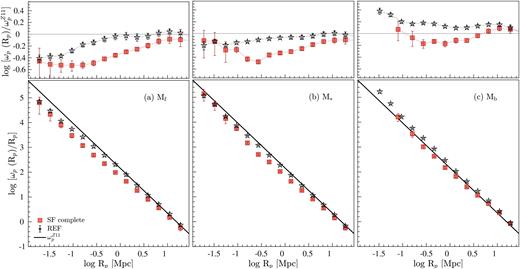
Main panels: The GAMA-projected ACFs of luminosity-selected (i.e. Mf, M*, and Mb, from the left- to right-hand side) REF (open black stars), and SF-complete (orange filled squares) samples covering the range 0.01 ≤ |$z$| ≤ 0.34. The black solid line denotes the empirical relation given in equation (8) (i.e. |$\omega _{\rm p}^{Z11}$|). Top panels: GAMA-projected ACFs relative to |$\omega _{\rm p}^{Z11}$|. The key is the same as that shown in the left-hand main panel.
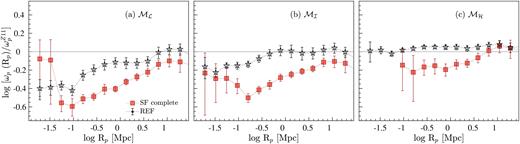
The GAMA-projected ACFs of REF (black open symbols) and SF-complete (orange filled symbols) stellar-mass-selected samples (i.e. |$\mathcal {M}_{L}$|, |$\mathcal {M}_{I}$|, and |$\mathcal {M}_{H}$|, from the left- to right-hand side) relative to |$\omega _{\rm p}^{Z11}$| (the key is shown in the left-hand panel).
In the range −0.15 ≲ log Rp (Mpc) ≲ 1.3, we find that the ACFs of REF and SF-complete galaxies, on average, are consistent with a power law. On smaller scales (log Rp ≲ −0.15 Mpc5), however, both sets of functions show varying levels of increase in the strength of clustering with decreasing Rp and optical brightness. This is most clearly evident in the ACFs|$_{\omega _{\rm p}^{Z11}}$| (i.e. top panels of Fig. 11) that demonstrate that at a fixed Rp, the amplitude of ACFs|$_{\omega _{\rm p}^{Z11}}$|increases with increasing optical brightness. This increase in amplitude appears to be stronger in the ACFs|$_{\omega _{\rm p}^{Z11}}$|of SF-complete galaxies than in REF functions on smaller scales, and vice versa on larger scales. Overall, the behaviour we see on larger scales (log Rp ≳ −0.15 Mpc) is consistent with other studies that report stronger clustering of massive and luminous galaxies than less massive, low-luminosity systems (e.g. Norberg et al. 2001; Zehavi et al. 2005b, 2011; Skibba et al. 2009; Marulli et al. 2013; Guo et al. 2014; Bray et al. 2015), and on smaller scales, the behaviour is mostly consistent with the results of another GAMA study by Farrow et al. (2015).
It is worth noting that even though the ACFs|$_{\omega _{\rm p}^{Z11}}$| of SF-complete galaxies show lower clustering amplitudes than their respective REF functions on most scales, the change in the strength of the ACFs|$_{\omega _{\rm p}^{Z11}}$| of SF-complete galaxies with decreasing Rp is greater than that of REF functions. In other words, the ACFs|$_{\omega _{\rm p}^{Z11}}$| of SF-complete galaxies show a steeper decline (increase) in strength at log Rp ≳ −0.15 Mpc (log Rp ≲ −0.15 Mpc) with decreasing Rp than REF functions. This rapid increase in the clustering strength of the ACFs|$_{\omega _{\rm p}^{Z11}}$| of SF-complete galaxies on smaller scales (i.e. excess clustering) suggests increased galaxy–galaxy interactions. The same behaviour is also apparent in the ACFs|$_{\omega _{\rm p}^{Z11}}$| of disjoint stellar-mass-selected samples of SF-complete galaxies (Fig. 12).
Interestingly, the Rp at which the ACFs|$_{\omega _{\rm p}^{Z11}}$| of SF-complete galaxies begin to show an increase in strength also seems to be optical-brightness-dependent, such that higher optical luminosities correspond to larger Rp and vice versa. For instance, the SF ACF|$_{\omega _{\rm p}^{Z11}}$| of Mf galaxies shows a turnover in the signal at ∼0.1 Mpc, though the signal appears to plateau6 at an Rp of ∼0.4 Mpc (or log Rp of −0.4). The SF ACFs|$_{\omega _{\rm p}^{Z11}}$| of M* and Mb show turnovers at larger Rp of ∼0.31 Mpc and ∼0.5 Mpc (i.e. log Rp of −0.51 and 0.3), respectively. This is in the sense that optically luminous SF galaxies show an enhancement in clustering at relatively larger separations than their low-luminosity counterparts.
As mentioned earlier, Rp provides an alternative metric to assess the interaction phase of a galaxy pair through the association of large Rp with time elapsed since or time to pericentric passage and small Rp with galaxies currently undergoing a close encounter. One of the advantages of using ACFs to trace the interaction phase is that, aside from the initial sample selection, ACFs are not affected by the properties of galaxies. As such, it is not the net change in a property with Rp that is being assessed, but the change in the clustering strength with Rp within the one- and two-halo terms. Interpreting the change in the strength of the clustering of ACFs|$_{\omega _{\rm p}^{Z11}}$| of SF-complete galaxies as a signature of increased interactions between galaxies, any correlation between optical brightness (or stellar mass) and Rp in which a change in the clustering signal takes place can be taken as a signature of a halo-size-interaction scale dependence. This suggests that the physical evidence of interactions between SF galaxies within massive haloes is (or ought to be) visible out to larger radii than those between star formers residing in less massive haloes. This is also supported by the fact that optically bright SF galaxies are likely hosted within massive haloes.
4.3 CCFs of SF galaxies
In this section, we extend the above analysis to further investigate the clustering properties of star formers with respect to different galaxy properties. For this, from each disjoint luminosity-selected (and stellar-mass-selected) sample, we draw subsamples containing the 30 % highest and the 30 % lowest sSFRs, (g − r)rest, D4000, and Balmer decrements. This selection is detailed in Section 2.4. The smaller 30 % samples increase the susceptibility of autocorrelation results to the effects of small number statistics; hence, we utilize cross-correlation techniques for the analyses presented in the subsequent sections. Note that all the CCF results shown in this paper correspond to cross-correlations between a given 30 % sample and its parent SF-complete sample. As part of this analysis, we also investigated the cross-correlations between a given 30 % sample and its parent REF sample, and we refer readers to Appendix C for a discussion of that investigation.
The CCFs of the 30 % highest and the lowest sSFR M* galaxies, and the 30 % bluest and the reddest (g − r)restM* galaxies are presented in the left-hand and right-hand panels of Fig. 13, respectively, where each 30 % sample is cross-correlated with its parent SF-complete sample. Also shown in the top panels of Fig. 13 are the CCFs relative to |$\omega _{\rm p}^{Z11}$|, hereafter CCFs|$_{\omega _{\rm p}^{Z11}}$|.
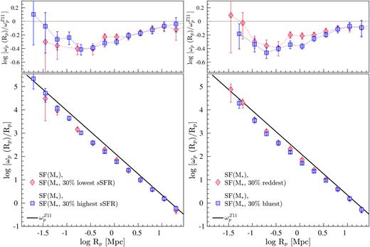
The projected CCFs of the 30 % subsets of M* SF-complete galaxies. Left-hand panels: The projected CCFs of the 30% highest (blue squares) and the 30 % lowest (red diamonds) sSFR galaxies (main panel), and the same functions relative to |$\omega _{\rm p}^{Z11}$| (top panel). Right-hand panels: The projected CCFs of the 30 % bluest (blue squares) and the 30 % reddest (red diamonds) galaxies in (g − r)rest (main panel), and the same functions relative to |$\omega _{\rm p}^{Z11}$| (top panel).
Most notable in Fig. 13 are, perhaps, the similar clustering excesses on small scales observed for the 30 % M* samples of high-sSFR, optically blue, and optically red galaxies. The overlap in clustering amplitudes between high-sSFR and optically blue galaxy populations is expected, given the correlation between sSFR and optical colour (Fig. 10). The overlap between the optically reddest and the highest SF populations again suggests that a significant fraction of the reddest M* galaxies in the SF-complete sample are in fact likely highly dust obscured high-sSFR galaxies or starbursts.
In Figs 14 and 15, we compare the CCFs|$_{\omega _{\rm p}^{Z11}}$| of all 30 % subsamples drawn from the three disjoint luminosity-selected SF-complete samples. The top panels of Fig. 14 present the CCFs|$_{\omega _{\rm p}^{Z11}}$| of high-sSFR galaxies and optically blue galaxies (blue and black symbols), and those of low-sSFR and optically red galaxies (red and black symbols) are presented in the bottom panels. To emphasize the degree of the enhancement of the clustering signal on small scales, we fit a linear relation to the log Rp < −0.64 Mpc data, where the dashed lines of the same colour denote the best-fitting linear relations to the data of the same colour. Likewise, the CCFs|$_{\omega _{\rm p}^{Z11}}$| of galaxies with low (high) D4000 indices and low (high) dust obscurations are presented in the top (bottom) panels of Fig. 15. In this figure, for reference, we overplot the best-fitting linear relations to the log Rp < −0.64 Mpc data shown in Fig. 14 as dashed lines.
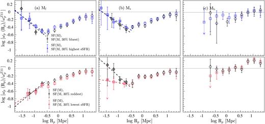
The projected CCFs of high-sSFR (low-sSFR) and optically blue (red) galaxies of luminosity-selected SF-complete samples relative to |$\omega _{\rm p}^{Z11}$| (optical luminosity increases from the left- to right-hand side). Top panels: the CCFs of optically blue (black diamonds) and high-sSFR (blue squares) galaxies. Bottom panels: the CCFs of optically red (black diamonds) and low-sSFR (red squares) galaxies. The dashed lines of the same colours denote the best-fitting linear relations to the Rp < 0.23 (log Rp < −0.64) Mpc data of the same colour. The data points used for the fitting are shown as filled squares, and the arrows denote the data with significant uncertainties.
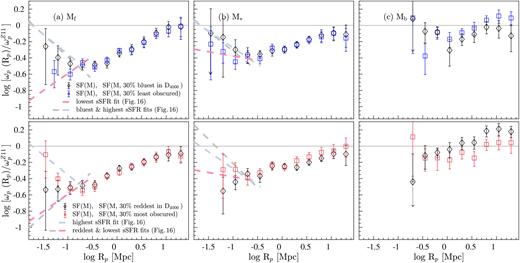
The projected CCFs of least (most) dust obscured and spectroscopically blue (red) galaxies of luminosity-selected SF samples relative to |$\omega _{\rm p}^{Z11}$| (optical luminosity increases from the left- to right-hand side). Top panels: the CCFs of least dust obscured (the 30 % of galaxies with the lowest Balmer decrement measures; blue squares) and spectroscopically blue (the 30 % with the lowest D4000 indices; black diamonds) galaxies. Bottom panels: the CCFs of most dust obscured (high Balmer decrement measures; red squares) and spectroscopically red (high D4000 indices; black diamonds) galaxies. For reference, we show the best-fitting linear relations shown in Fig. 14 as dashed lines.
In the range −0.52 ≲ log Rp [Mpc] ≲ 1.3, all CCFs|$_{\omega _{\rm p}^{Z11}}$| show a progressive decline in the strength of clustering with decreasing Rp. The clustering amplitudes of low-sSFR and optically red galaxies over this range are, on average, higher than that of their respective high-sSFR and optically blue counterparts, in agreement with the studies that find high-sSFR galaxies are less clustered than their low-sSFR counterparts (e.g. Mostek et al. 2013; Coil et al. 2016), as well as with the studies that find higher clustering strengths for optically redder galaxies versus optically bluer systems (e.g. Zehavi et al. 2011; Ross et al. 2014; Favole et al. 2016).
Interestingly, on small scales (i.e. log Rp ≲ −0.52 Mpc), we see a discrepant behaviour between the CCFs|$_{\omega _{\rm p}^{Z11}}$| of optically red galaxies of different luminosity-selected samples. The most notable is the CCFs|$_{\omega _{\rm p}^{Z11}}$| of Mf galaxies that show a continuous decline in clustering strength with decreasing Rp, whereas the respective CCFs|$_{\omega _{\rm p}^{Z11}}$| of M* and Mb galaxies suggest otherwise. These differences can shed light into dust build-up and destruction mechanisms in optically faint (low-mass) versus bright (massive) SF galaxies. At a fixed SFR, an optically faint galaxy would be classified as a starburst, while a luminous system would appear as a normal (or a low) star former (see the distribution of the constant log SFR contours in Fig. 10). Therefore, to gain further insights into these differences, we add an analysis based on D4000 and Balmer decrements (Fig. 15), which are complementary to sSFR and (g − r)rest, to this study.
The D4000 spectral index is a diagnostic of cumulative star formation history of a galaxy, where lower D4000 indices are indicative of younger stellar populations and vice versa, and is therefore considered a proxy for (g − r)rest (Fig. 9). For ease of comparison with the optical colour based analysis discussed above, we hereafter refer to galaxies with lower (higher) D4000 indices as spectroscopically blue (red).
The principal advantage of using D4000 is that it is less sensitive to dust reddening than (g − r)rest7. Secondly, it is a spectroscopy-based quantity. In the case of single-fibre spectroscopy, the spectrum of a galaxy represents the central region where interaction-triggered starbursts are likely to occur (Mihos & Hernquist 1996; Di Matteo et al. 2007; Montuori et al. 2010), whereas photometry-based colours represent the light from the whole galaxy. Therefore, in galaxies undergoing interactions with likely centrally triggered dusty starbursts, the correlation between SFR and D4000 can be stronger than that between SFR and (g − r)rest. Indeed this is evident in Fig. 15. The CCF|$_{\omega _{\rm p}^{Z11}}$| of spectroscopically red M* galaxies shows a continuous decline in strength at log Rp ≲ −0.64 Mpc, whereas the opposite is observed for optically red M* galaxies. In comparison to the CCFs|$_{\omega _{\rm p}^{Z11}}$| of optically red Mf galaxies, the CCFs|$_{\omega _{\rm p}^{Z11}}$| of spectroscopically red Mf galaxies too show some differences, though within uncertainties the two CCFs|$_{\omega _{\rm p}^{Z11}}$| are in agreement. According to these results, the D4000 index appears to be more useful in discriminating starbursts than optical colours. Even though fibre colours are still more susceptible to dust effects than D4000, the correlation between fibre colour and SFR can be stronger than that between global colour and SFR.
The dust obscuration in SF galaxies has been observed to depend on both galaxy SFR and stellar mass (e.g. Brinchmann et al. 2004; Garn & Best 2010; Zahid et al. 2013). Dust is theorized to build up rapidly during a starburst (Hjorth et al. 2014), while a quiescently star forming galaxy experiences a simultaneous decline in dust and SFR as a result of dust destruction and diminishing gas supply (da Cunha et al. 2010). The CCFs|$_{\omega _{\rm p}^{Z11}}$| of both most and least dust obscured galaxies (Fig. 15) show enhancements in clustering amplitudes with decreasing log Rp at ≲ − 0.64 Mpc. As shown in Fig. 1, the SF galaxies can have a range of dust obscurations, which can explain the similar enhancements in clustering observed for most and least dust obscured SF populations of the luminosity-selected samples. The clustering excess observed for most dust obscured M* galaxies further supports our earlier assertion that the increase in clustering amplitude of optically red M* galaxies (Fig. 13) is, at least in part, caused by the presence of dusty starbursts.
In the range −0.52 ≲ Rp [Mpc] ≲ 1.3, the CCFs|$_{\omega _{\rm p}^{Z11}}$| of the most (least) dust obscured Mf and M* galaxies agree qualitatively with the high-sSFR (low-sSFR) counterparts, as well as with the CCFs|$_{\omega _{\rm p}^{Z11}}$| of spectroscopically blue (red) galaxies. The Mb CCFs|$_{\omega _{\rm p}^{Z11}}$| of the most and least dust obscured star formers, on the other hand, show an agreement with that of high-sSFR Mb galaxies.
For completeness, we present the CCFs|$_{\omega _{\rm p}^{Z11}}$| of high-SFR (low-SFR) and optically blue (red) galaxies of the three disjoint stellar-mass-selected samples (Table 2) in Fig. 16. The dashed lines are the same as in previous figures. These results are, as expected, largely comparable to that observed for high-sSFR (low-sSFR) and optically blue (red) galaxies of luminosity-selected samples, and as such, we do not discuss them separately here.
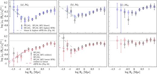
The projected CCFs of high-SFR (low-SFR) and optically blue (red) galaxies of stellar-mass-selected SF galaxies relative to |$\omega _{\rm p}^{Z11}$| (Table 2; stellar mass increases from the left- to right-hand side). Top panels: the CCFs of high-SFR (blue squares) and optically blue (black diamonds) galaxies. Bottom panels: the CCFs of low (red squares) and optically red (black diamonds) galaxies. For reference, we show the best-fitting linear relations shown in Fig. 14 as dashed lines.
Finally, we also perform a volume-limited cross-correlation analysis, the results of which are presented and discussed in Appendix B2. Briefly, the CCFs|$_{\omega _{\rm p}^{Z11}}$| of volume-limited samples show a qualitative agreement with their respective non-volume-limited counterparts on most scales. There are some quantitative differences between the two sets of CCFs|$_{\omega _{\rm p}^{Z11}}$| on smaller scales, which rise as a result of small number statistics.
4.4 The rank-ordered mark correlation functions of star forming galaxies
The mark clustering statistics are different from the auto- and cross-correlation techniques discussed in the previous sections. The mark statistics can shed light on the dependence of a given physical property on the separation of a galaxy pair by weighting each galaxy in that pair by that physical property. Given this sensitivity of MCFs to environmental effects, they form a useful tool in identifying and quantifying underlying correlations of various galaxy properties with the environment.
In conventional mark two-point clustering statistics, the correlation function is directly weighted by a given mark, i.e. a physical property (e.g. SFR, sSFR). Consequently, the amplitude of an MCF depends not only on the distribution of marks (Skibba et al. 2006, 2009), but also on the differences in the formulation of a mark (e.g. log or linear; Skibba et al. 2006, 2009). Therefore, unless the distributions of different marks are similar, different MCFs cannot be compared with each other to understand the dependence of different galaxy properties on the galaxy separation. In our case, the SFR, sSFR, and (g − r)rest distributions of SF-complete samples used differ in shape, magnitude, and range. As such, in order to compare the SFR, sSFR, and (g − r)rest MCFs, we rank-order the marks and use the rank as the mark. This method, introduced in Skibba et al. (2013), allows the effects of the shape of the distribution on the strength of the MCF to be removed, such that a mark correlation signal can be compared between different marks. The caveat of this method is that any information contained in the shape of a distribution will be lost.
We present the rank-ordered sSFR and (g − r)rest MCFs of luminosity-selected (top panels), and rank-ordered SFR and (g − r)rest MCFs of stellar-mass-selected (bottom panels) SF-complete samples in Fig. 17. On small scales, the rank-ordered sSFR and SFR MCFs indicate a clear enhancement in amplitude compared to that of (g − r)rest MCFs. This suggests that sSFR and SFR correlation signals indeed correlate more strongly with the environment than optical colour. The decrement in sSFR, SFR, and (g − r)rest mark correlation signals in the range −0.82 ≲ log Rp [Mpc] ≲ 0.6, which is more strongly evident in rank-ordered MCFs of Mf and |$\mathcal {M}_{\mathcal {L}}$| galaxies, likely demonstrates the effects of post-starbursts, where certain physical properties of a galaxy, e.g. SFR and colour, are affected by the increased presence of now ageing stellar population produced during a starburst.
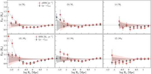
The rank-ordered MCFs of luminosity-selected (top row; optical luminosity increases from the left- to right-hand side) and stellar-mass-selected (bottom row; stellar mass increases from the left- to right-hand side) SF-complete samples. The orange and grey filled symbols in the top panels denote the rank-ordered sSFR and (g − r)rest MCFs, respectively, and in the bottom panels they denote SFR and (g − r)rest MCFs, respectively. The shaded regions indicate the scatter from randomizing the marks.
For completeness, we also present and discuss the conventional MCFs in Appendix D (Figs D1 and D2). The most notable in the conventional case is the strengthening in clustering amplitude with increasing optical brightness observed for sSFR and SFR populations, which mirrors that observed in ACFs and CCFs presented in previous sections.
5 DISCUSSION
In this study, we considered several different SF properties of galaxies (i.e. SFR, sSFR, (g − r)rest, D4000, and Balmer decrement), which are most likely to be affected by galaxy–galaxy interactions. We utilized the [O iii] λ5007 Å/Hβ and [N ii] λ6584 Å/H α diagnostics (i.e. BPT, Baldwin et al. 1981), which can be used as an indicator of gas-phase metallicity, to demonstrate the variation of the physical properties considered with metallicity in SF galaxies (Figs 8–10). In general, the variation in sSFR largely mirrors that of (g − r)rest and D4000, where low sSFRs are typically characterized by lower metallicities. Dust obscuration, on the other hand, indicates a variation similar to that seen with SFR, where high-SFR galaxies show a higher dust obscuration than low-SFR systems.
Below we discuss the main findings of this study and is structured as follows. A discussion of the results of auto-, cross-, and mark-correlation analyses of SF galaxies is presented in Sections 5.1–5.4, and in Section 5.5, we compare the GAMA results of this study with that of SDSS.
5.1 On the potential interaction-scale halo-size dependence of interaction-driven disturbances
The role that a large-scale environment plays in driving and sustaining changes induced during a galaxy–galaxy interaction is understood to a lesser extent than the role of the interaction itself. Generally, the net changes in physical properties of galaxies are used as direct indicators of interactions and environmental effects. As mentioned before, the focus of our study is to explore the suitability of utilizing two-point correlation statistics to shed light on any dependence of galaxy–galaxy interactions on their large-scale (i.e. halo-scale) environment. For this, we have computed two-point ACFs, CCFs, and MCFs of SF galaxies as a function of both optical luminosity and stellar mass, which approximately correlate with halo mass.
In order to quantify the Rp out to which signatures of interactions ought to persist, in Section 4.2, we make the assumption that any change in the relative strength of clustering of a given population reflects its interaction scale.8 For example, the ACFs of both luminosity- and stellar-mass-selected SF galaxies are consistent with a power law in the range −0.15 ≲ log Rp [Mpc] ≲ 1.3. At log Rp ≲ −0.15 Mpc, they show a significant clustering excess (Fig. 11). This is best seen in ACFs|$_{\omega _{\rm p}^{Z11}}$|, where this change appears as a turnover in the signal. It is this ‘turnover’ that we consider to approximately correspond to the interaction scale of that galaxy population. The interaction scales estimated this way appear to depend on galaxy luminosity. This is in the sense that the interaction scale of optically brighter SF galaxies is greater than that of optically faint galaxies. This could be interpreted as a signature of a halo-size-interaction scale dependence, where the evidence of interactions between star formers residing in massive haloes is visible out to larger radii than those between star formers residing in low-mass haloes. This can be, in part, due to massive haloes playing a greater role in enhancing and sustaining the effects of galaxy interactions than their less massive counterparts. Equally, this could also be an artefact of high-mass inhabitants of massive haloes being able to form stars more efficiently than low-mass galaxies in interactions ( Ferreras et al. 2017).
The ACFs of both luminosity- and stellar-mass-selected REF galaxies also show similar changes in the small-scale clustering. These changes are, however, not as significant as those observed in SF galaxies. In comparison to the ACFs of REF galaxies, the star formers show lower clustering amplitudes over most scales, except at log Rp ≲ −0.15 Mpc. At log Rp ≲ −0.15 Mpc, the ACFs of SF galaxies show a rapid increase in the amplitude of clustering with decreasing Rp. Consequently, over these scales, the clustering of SF galaxies appears to be similar to that of REF. Both these results are consistent with the findings of previous studies: the former with the studies that find optically redder galaxies are more strongly clustered than their bluer counterparts (e.g. Zehavi et al. 2005b, 2011; Skibba et al. 2009; Bray et al. 2015) and the latter with the Farrow et al. (2015) clustering study of optically selected red and blue galaxies, finding an upturn in the clustering of the blue systems on small scales, as well as with the results of Heinis et al. (2009) and Mostek et al. (2013).
5.2 On the direct indicators versus two-point correlation statistics tracing interaction scales
Here we discuss the potential reasons for the differences in Rp reported by the studies that utilize direct probes of interactions (see Section 1 for a discussion), as well as between those and the predictions of our autocorrelation analysis.
A vast number of competing factors can influence both the strength of an interaction-induced physical change and the Rp out to which the net effect is observable. The orbital parameters, for instance, can play a significant role in moderating the SFR response. Both observational and theoretical studies suggest that retrograde encounters lead to higher star formation efficiencies, and thus higher SFR enhancements, than prograde encounters (Di Matteo et al. 2007; Mesa et al. 2014). The ratio of the stellar masses of the progenitors and their gas fractions are two other factors that can significantly influence the strengths of direct indicators. Galaxy pairs with mass ratios between 1 and 3 are observed to have the strongest SFR enhancements (e.g. Cox et al. 2006; Ellison et al. 2008). Likewise, lower gas fractions are theorized to lead to lower SFR enhancements (Di Matteo et al. 2007). While starbursts with the shortest durations tend to typically show the strongest enhancements (Di Matteo et al. 2007) and tend to occur over the smallest separations (typically <|$30\, h^{-1}_{70}$| kpc; e.g. Ellison et al. 2008; Li et al. 2008a; Wong et al. 2011; Scudder et al. 2012; Patton et al. 2013), the smallest separations can also inhibit SFR if the tidal forces are strong enough to eject molecular gas into tidal tails without allowing the gas to funnel to the centres of galaxies (Di Matteo et al. 2007). Overall, these competing effects can ‘wash out’ the net signal of direct indicators, thus affecting the observability of a physical change.
The differences in dynamical time-scales associated with different star formation probes are another factor that must be considered when using physical properties as tracers of interactions. Davies et al. (2015), based on the GAMA survey data, report that short-duration star formation indicators show stronger signs of enhancement/suppression than long-duration tracers. The H α SFR, for example, is a direct tracer of ongoing star formation in galaxies, probing on average the star formation over a shorter time-scale (i.e. ∼10 Myr) than broad-band photometry, e.g. (g − r) probes star formation over much longer time-scales of ∼1 Gyr. The short-duration indicators are, therefore, expected to be most vulnerable to recent dynamical events. This suggests that the dynamical time-scales of processes that likely trigger short-duration star formation events are also shorter than those of processes that likely trigger long-duration events. The implication is that analyses that rely on observations of net changes are susceptible to the differences in the dynamical time-scales of physical processes that trigger and sustain different changes. This can, perhaps, further explain the differences in the reported interaction scales. In this sense, autocorrelation techniques offer an alternative to trace interaction scales that is almost9 independent of the influences of interaction-induced direct observables.
A dependence on the interaction scale and the size of a halo suggests that star formation activity evolves differently in different environments. Elbaz et al. (2007) and Ziparo et al. (2014) report a reversal of the SFR–density relationship at |$z$| ∼ 1, from high-density environments hosting high-SFR galaxies at earlier times to low-density environments hosting high-SFR systems at later times. Popesso et al. (2015a,b) interpret SFR–density relation and ‘galaxy downsizing’ (Cowie et al. 1996) in terms of ‘halo downsizing’, where the SFR contribution of massive haloes to the cosmic SFR density becomes progressively less significant with increasing cosmic time. In the local Universe, the bulk of the stellar mass is locked in galaxy groups (Eke et al. 2005) so that group-sized haloes are the most common type of haloes for an SF galaxy to inhabit. Therefore, it is likely that most of the aforementioned studies preferentially selected galaxies residing in one type of a halo (i.e. group-sized haloes) over the others. In our study, by using disjoint luminosity-selected and stellar-mass-selected samples, we attempt to minimize this preferential selection, as well as the overlap between haloes of different sizes, thereby giving insight into interactions between star formers in relatively low- versus high-mass haloes.
5.3 On the use of cross-correlation techniques in the determination of interaction scales with respect to galaxy properties
As mentioned earlier, galaxy–galaxy interactions have been observed to drive many physical changes in galaxies. The best physical tracer of an interaction can, however, differ depending on the progenitors, the environment, and the interaction itself. It has been shown, both theoretical and observationally, that SF–SF galaxy pairs largely favour low-to-moderate density environments, which are typical hosts to low-mass galaxies with higher gas fractions, whereas non-SF–non-SF and SF–non-SF galaxy pairs are preferentially found in high-density environments (e.g. Ellison et al. 2010; Lin et al. 2010). As such, while interactions still occur in high-density environments, they may not always lead to an enhancement in star formation (Ellison et al. 2008, 2010), though can, perhaps, lead to a change in another property such as optical colours. Below we discuss the clustering properties of SF galaxies in different environments with respect to different SF properties of galaxies obtained from the cross-correlation analysis presented in Section 4.3.
On small scales, the CCFs|$_{\omega _{\rm p}^{Z11}}$| of Mf star formers of high (low) sSFRs, high (low) dust obscurations, and bluer (redder) optical and spectroscopic colours show enhancements (decrements) of varying degrees in clustering amplitudes with decreasing Rp (Figs 14 and 15). In contrast, all CCFs|$_{\omega _{\rm p}^{Z11}}$| of SF M* galaxies, except spectroscopically red objects, show enhancements. The most notable are the opposing clustering trends observed between optically red Mf versus M* populations, and likewise between spectroscopically red (i.e. higher D4000 indices) and optically red M* populations. As D4000 is less sensitive to dust effects than optical colours, one of the potential drivers of these discrepancies is dust obscuration.
The clustering excess observed for highly dust obscured M* galaxies and the dearth in clustering observed for spectroscopically red galaxies support the assertion that a large fraction of optically red SF M* galaxies are likely dusty starbursts. To illustrate this further, in Fig. 18, we show the distribution of sSFRs as a function of |$250\, \mu$|m luminosity10 (L250 [W Hz−1]) for all optically red Mf and M* star formers detected in Herschel 250 |$\mu$|m photometry. The colour code denotes mean dust obscuration as measured by Balmer decrement, and black and red contours indicate the distribution of the 30 % reddest Mf and M* galaxies, respectively. The sSFR cuts used to select the 30 % highest sSFR galaxies from Mf and M* samples are shown by the dashed lines. The significant overlap between the high-sSFR and optically red M* populations demonstrates that the redder optical colours of these SF systems have been enhanced by dust.
![The $\log L_{\rm {250}}\, [\rm W\, Hz^{-1}]$ and $\log\,{\rm sSFR}\, [\rm yr^{-1}]$ distribution of the 30 % reddest Mf and M* galaxies of the SF-complete sample, colour-coded by mean dust obscuration (as measured by the Balmer decrement, i.e. BD). The contours enclose 25, 50, and 75% of the data, and the dashed lines denote the approximate cuts in log sSFR used to select the 30 % highest sSFR Mf (black) and M* (red) galaxies.](https://oup.silverchair-cdn.com/oup/backfile/Content_public/Journal/mnras/479/2/10.1093_mnras_sty1638/1/m_sty1638fig18.jpeg?Expires=1750475624&Signature=hCQOYuLz5bMTbHVHkhTVyUR6VW9BI~lZ65AGMGrQHC0jUa-oB7274-P9g5cFTI-91nQ0eUYkNoK2HXpsYEVRJNLqMxsWLBZ-MQMaZ67TlXMzHDq0S3v0i3K9i2dNO3D4wfNujh3fT9YYGS8BuMJxEKLMON30GzHeAGVJz0WV1rx--zXKcCDA9PSmtPJU1W~ukGXD88hTVtkp875TiglwjAdPGbBX7EqXu0SdmobTKlVRoaJdzcfmyW6pO1AU-Wae8EkSdNruIOFnU161TXrvJycefV~KZc-4988YfBeGyifGBc~QNrNHXWLkq1YSC9t-7bE6oZK4-ivnPrxzsbJOMQ__&Key-Pair-Id=APKAIE5G5CRDK6RD3PGA)
The |$\log L_{\rm {250}}\, [\rm W\, Hz^{-1}]$| and |$\log\,{\rm sSFR}\, [\rm yr^{-1}]$| distribution of the 30 % reddest Mf and M* galaxies of the SF-complete sample, colour-coded by mean dust obscuration (as measured by the Balmer decrement, i.e. BD). The contours enclose 25, 50, and 75% of the data, and the dashed lines denote the approximate cuts in log sSFR used to select the 30 % highest sSFR Mf (black) and M* (red) galaxies.
Finally, the differences in the environments typically inhabited by optically faint versus bright galaxies provide another explanation for the differences between CCFs. The galaxy–galaxy interactions in higher density environments have been observed to lead to quenching of ongoing star formation, thus amplifying their redder colours (Ellison et al. 2010; Patton et al. 2011). These interactions likely also play a role in enhancing the redder colours of optically brighter galaxies that generally reside in denser environments than optically fainter systems.
5.4 On the use of mark-correlation techniques in the determination of interaction scales
The mark-correlation statistics allow for the dependence of interaction scale on galaxy properties to be investigated. In mark statistics, unlike in cross-correlation analysis, the galaxies are weighted directly either by a given physical property or by a rank-order assigned to them based on the distribution of a given physical property. We compute MCFs using both these methods. The results based on the former (i.e. the conventional) method are presented in Appendix D, and they allow the comparison of MCFs of the same mark between different galaxy samples. Those based on the latter are shown in Fig. 17, and permits the comparison of MCFs of different marks between different galaxy samples.
The sSFR and (g − r)rest MCFs based on the conventional method show a strengthening in the mark-correlation signal with decreasing Rp, and at a fixed Rp, the strength increases with increasing optical brightness. The same trend is also evident with increasing stellar mass in the SFR and (g − r)rest MCFs of stellar-mass-selected SF-complete samples. The greater enhancement in sSFR observed in the MCF of M* galaxies than that of Mf galaxies (Fig. D1) is in agreement with that expected if the fraction of dusty starbursts with M* luminosities is higher than those with optically fainter luminosities.
Finally, the comparison of rank-ordered MCFs of sSFR, SFR, and (g − r)rest galaxies shows that the relative mark-correlation strengths of sSFR MCFs are higher than those of the respective (g − r)rest functions across all luminosity-selected SF-complete samples. Likewise, the mark-correlation strengths of SFR MCFs are higher that of the respective (g − r)rest across all stellar-mass-selected SF-complete samples. This suggests that sSFR and SFR are more sensitive probes of the effects of interactions than optical colours, in agreement with the findings of Heinis et al. (2009).
5.5 A comparison between SDSS and GAMA
The CCFs|$_{\omega _{\rm p}^{Z11}}$| of GAMA and SDSS (Li et al. 2008a) high- and low-sSFR galaxies are presented in Fig. 19. Li et al. (2008a) define high- and low-sSFR galaxies as those within the upper and lower 25th percentiles of the sSFR distribution, and they cross-correlated with a reference sample containing galaxies in the ranges 0.01 ≤ |$z$| ≤ 0.3 and −23 ≤ Mr ≤ −17. Therefore, in order to make this comparison as fair as possible, the GAMA CCFs|$_{\omega _{\rm p}^{Z11}}$| shown in Fig. 19 are the CCFs|$_{\omega _{\rm p}^{Z11}}$| obtained from cross-correlating SF-complete samples with their respective REF samples (see Appendix C for the cross-correlation analysis involving REF samples). In general, the SDSS CCFs|$_{\omega _{\rm p}^{Z11}}$| of high sSFR show a good agreement with that of GAMA high-sSFR M* galaxies. The low-sSFR SDSS function, on the other hand, exhibits a lower clustering strength than the GAMA functions, which is most likely a result of the differences between galaxy samples used for the two studies. For example, even though we show the results of the cross-correlation between SF and REF samples in Fig. 19, the redshifts and optical luminosities spanned by the galaxy samples used by Li et al. (2008a) are still larger than the ranges that we considered for our analysis.
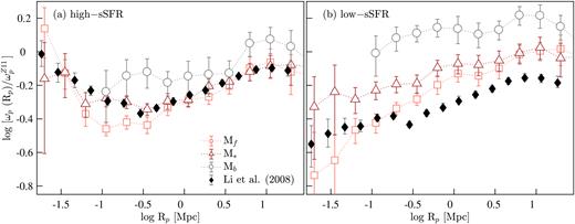
The projected REF CCFs of high-sSFR (open squares; left-hand panel) and low-sSFR (open squares; right-hand panel) Mf, M*, and Mb galaxies relative to |$\omega ^{Z11}_{\rm p}$|. The filled symbols denote the Li et al. (2008a) CCFs of high-sSFR (left-hand panel) and low-sSFR (right-hand panel) SDSS galaxies. Li et al. (2008a) define high- and low-sSFR galaxies as galaxies contained in the upper and lower 25th percentiles of the distribution of sSFRs of galaxies in the ranges 0.01 ≤ |$z$| ≤ 0.3 and −23 ≤ Mr ≤ −17.
In Fig. 20, we compare the GAMA sSFR MCFs with the SDSS measures provided in Li et al. (2008a). Relative to GAMA, the enhancement in sSFR of SDSS galaxies occurs at a smaller Rp, and the amplitude at a fixed Rp is lower than that of GAMA Mf and M* sSFR MCFs. Moreover, the GAMA sSFR MCFs of Mf and M* galaxies show a strengthening in the mark-correlation signal with increasing optical luminosity and/or redshift. The enhancement in sSFR of SDSS galaxies also appears to support this trend, suggesting that interactions between luminous galaxies trigger more intense starbursts than those between faint systems.
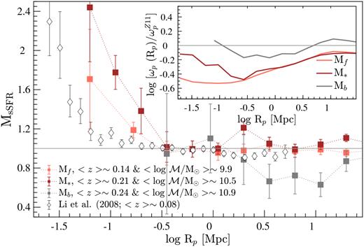
GAMA versus SDSS sSFR MCFs. The GAMA MCFs of Mf, M*, and Mb galaxies (filled symbols) in comparison to the sSFR-enhancement functions of SDSS |$-23\le M_{r_{0.1}} \le -17$| galaxies extended over the range 0.01 ≤ |$z$| ≤ 0.3, where |$M_{r_{0.1}}$| are r-band absolute magnitudes k-corrected to |$z$| = 0.1 (Li et al. 2008a). The mean redshift and stellar mass coverages of each galaxy sample are given in the legend.
We show the GAMA ACFs|$_{\omega _{\rm p}^{Z11}}$| (Section 4.2) in the inset of Fig. 20 for comparison. On average, the Rp at which the sSFR MCFs of the three luminosity-selected SF-complete samples show an enhancement in sSFR appears to coincide with the Rp at which the respective ACFs|$_{\omega _{\rm p}^{Z11}}$| begin to show a change. This result is not unexpected as MCFs are in a sense ACFs with weights based on the galaxy properties applied.
6 SUMMARY
We have used a sample of galaxies with detected H α emission drawn from the GAMA survey to study the small-scale clustering properties of SF galaxies as a function of both optical luminosity and stellar mass. In the process, we provide a method using which the random clones of galaxies computed by Farrow et al. (2015) for the GAMA survey (i.e. computed for a galaxy survey with a univariate primary selection) be applied to a bivariately selected sample of galaxies (e.g. an SF sample of galaxies drawn from a broad-band survey). The autocorrelation, cross-correlation, and two-point mark-correlation techniques have been used in the computation of galaxy correlation functions for each luminosity- and stellar-mass-selected sample, and below we summarize the main conclusions of this study.
The strengthening of clustering on small scales observed in GAMA ACFs of star formers (Section 4.2) is a signature of galaxy–galaxy interactions.
With increasing optical brightness, the increase in the clustering amplitude of SF population with decreasing Rp at a given Rp (log Rp ≲ −0.15 Mpc) becomes progressively more significant, and the Rp at which the clustering signal of the ACFs of SF galaxies relative to the fiducial power law shows a turnover becomes progressively larger. This behaviour of SF galaxies can be interpreted as evidence of an existence of an interaction scale, where physical changes induced in an interaction are, or rather ought to be, evident out to the Rp at which the clustering signal of a given SF population relative to the fiducial power law starts to alter. This is in the sense that the interactions between optically bright galaxy pairs induce changes that are evident out to larger separations than those between optically faint galaxies.
The main advantage of utilizing autocorrelation techniques to map interaction scales is that they are much less susceptible to (1) fluctuations (i.e. enhancements and decrements) in measured properties, (2) the observability of a change (i.e. the change in a physical property can be too subtle to be observable over some scales), and (3) the differences arising from the type of star formation indicator used (e.g. short- versus long-duration star formation indicators) than methods that employ net changes in properties to trace interactions.
Out of the different potential signatures of interactions (e.g. sSFR, SFR, optical colour, D4000, and Balmer decrement) considered in this study, the clustering with respect to (30 per cent) sSFR and SFR, both based on H α emission, on average shows the strongest small-scale enhancements across all magnitude and stellar mass ranges considered. Likewise, the 30 % lowest sSFR and SFR galaxies show a decrement in clustering across all magnitude and stellar mass ranges.
The optical colours, i.e. (g − r)rest, can be affected by the dust obscuration in galaxies. The spectroscopically based D4000 indices, a proxy for colour that is less affected by dust and in single-fibre spectroscopy represents the changes in central regions of galaxies, can provide a clearer picture of the effects of interactions than optical colours.
The comparison between rank-ordered sSFR and (g − r)rest MCFs shows that the small-scale enhancement in sSFR is stronger than that of (g − r)rest, supporting the aforementioned conclusion that sSFR is a better tracer of interactions between SF galaxies than other tracers considered.
The sSFR MCFs show an increase in small-scale clustering, and the amplitude at a given Rp of the MCF of optically bright (e.g. M*) sSFR galaxies greater than that of optically faint (e.g. Mf) sSFR systems. This suggests that optically brighter SF systems are characterized by a higher SFR than fainter objects. Based on the comparison of dust properties of different SF populations, it is clear that optically bright high-SFR systems contain higher dust contents than their fainter counterparts.
Highly complete data sets with large redshift coverage that will be provided by the future/planned galaxy surveys will allow further insights into the relationship between interaction scale and optical brightness, and into underlying physical processes (galaxy and/or cluster scale) that are responsible for it. Moreover, these data sets will allow any evolution in interaction scales to be tightly constrained, thereby shedding light on the evolution of physical properties and processes of galaxies across time.
ACKNOWLEDGEMENTS
We thank Ignacio Ferreras, Jarle Brinchmann, and Nelson Padilla for valuable discussions. We also thank the anonymous referee for their careful reading of this manuscript and helpful comments, which improved the presentation of this paper.
MLPG acknowledges the support from a CONICYT-Chile grant FONDECYT 3160492, and has also received funding from the European Union’s Horizon 2020 research and innovation programme under the Marie Skłodowska–Curie grant agreement No 707693. MLPG, PN, and IZ acknowledge support from a European Research Council Starting Grant (DEGAS-259586). PN acknowledges the support of the Royal Society through the award of a University Research Fellowship and the support of the Science and Technology Facilities Council (ST/L00075X/1). IZ is supported by NSF grant AST-1612085.
GAMA is a joint European–Australasian project based around a spectroscopic campaign using the Anglo-Australian Telescope. The GAMA input catalogue is based on data taken from the SDSS and the UKIRT Infrared Deep Sky Survey. Complementary imaging of the GAMA regions is being obtained by a number of independent survey programmes, including GALEX MIS, VST KIDS, VISTA VIKING, WISE, Herschel-ATLAS, GMRT, and ASKAP providing UV to radio coverage. GAMA is funded by the STFC (UK), the ARC (Australia), the AAO, and the participating institutions. The GAMA website is http://www.gama-survey.org/.
Data used in this paper will be available through the GAMA website (http://www.gama-survey.org/) once the associated redshifts are publicly released.
This work used the DiRAC Data Centric system at Durham University, operated by the Institute for Computational Cosmology on behalf of the STFC DiRAC HPC Facility (www.dirac.ac.uk). This equipment was funded by a BIS National E-infrastructure capital grant ST/K00042X/1, STFC capital grant ST/K00087X/1, DiRAC Operations grant ST/K003267/1, and Durham University. DiRAC is part of the National E-Infrastructure.
Footnotes
The rest-frame colours used in this analysis are based on these absolute magnitudes.
In cases where an object has an independent GAMA and a SDSS spectrum, the SDSS spectrum is generally found to have the highest spectral signal-to-noise ratio, and is selected to be part of the sample.
Emission-line samples drawn from a broad-band survey, like GAMA, can be biased against low-SFR and weak-line systems. This can become significant with increasing redshift and apparent magnitude, and the differences in clustering results obtained from different clustering estimators can be used to quantify the significance of such biases.
This completeness is achieved through excluding very low SFR sources as they can significantly limit the redshift coverage of a volume-limited sample, resulting in samples with small number statistics.
Corresponds to an Rp of ≲ 0.7 Mpc.
Plateau here implies that the ACF has the same gradient as |$\omega _{\rm p}^{Z11}$|.
The D4000 measures used for this study are based on the Balogh et al. (1999) definition, which samples a very narrow range in wavelength.
We use the term ‘interaction scale’ to denote the Rp out to which changes in physical properties ought to be evident instead of ‘observable time-scale’ to avoid confusion, as this term is generally used by studies that rely on net changes in physical properties to trace interactions.
As we have used H α fluxes to select the SF sample used for this analysis, our results are not completely independent.
The Herschel 250 |$\mu$|m photometry is drawn from HATLASCatv03 (Smith et al. 2011).
REFERENCES
APPENDIX A: ON THE MODELLING OF THE SURVEY SELECTION FUNCTION AND ON THE IMPACT OF SAMPLE SYSTEMATICS
A1 Modelling of the survey selection function in redshift bins
We describe the modelling of the selection function used for the analysis presented in Section 3.1, which is based on equation (1) with Vzlim set either to the redshift detection limit of 0.34 of the H α spectral feature in GAMA spectra or to |$z$| ∼ 0.24. Alternatively, the Nweights can also be computed in redshift slices such that Vzlim defines the volume of a given redshift slice. Fig. A1 shows the distributions Ngalaxies in redshift bins, where Nweights computed in redshift slices are used to weight the random galaxies. Note that the redshift ranges are defined such that none includes the redshift band centred around |$z$| ∼ 0.16.
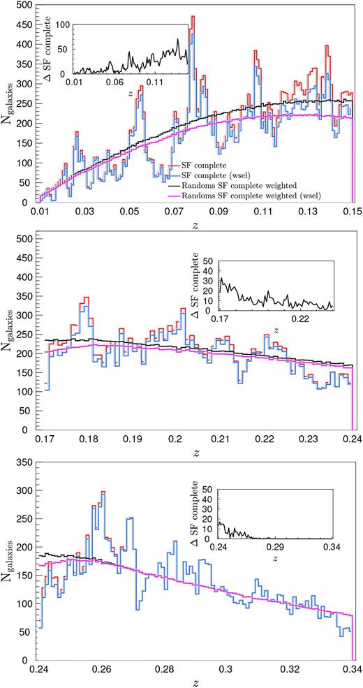
The redshift distributions of SF-complete galaxies in comparison to the weighted and weight-selected, where galaxies with Nweights > 10 are removed from the sample, distributions of the equivalent random galaxies. The randoms are weighted by Nweights computed in redshift slices, and each inset shows the difference between SF complete and SF complete (wsel).
Fig. A2 shows the mean distribution of Nweights with respect to both SFR and optical luminosity. As discussed in this paper, the Vmax of each galaxy is used in the computation of its Nweight, and Vmax can either be limited by the galaxy’s SFR (i.e. H α flux), or by its r-band magnitude or by the upper limit of the relevant redshift slice. The solid red lines show approximate regions in the SFR and Mr plane where a galaxy with a given Nweight lies if the Vmax of that galaxy is limited by its SFR (lower regions), by r-band magnitude (upper region), or by the upper redshift limits of the relevant redshift bin (leftmost region). The main caveat of the calculation of Nweights in redshift slices is that due to the relatively narrow range in redshift sampled a large fraction of galaxies are assigned Nweights > 10.
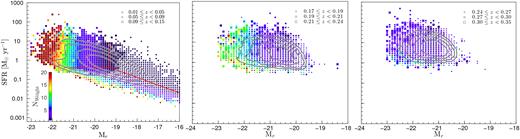
The weights applied to the galaxies in random SF complete as a function of SFR and Mr in the ranges 0.01 ≲ |$z$| < 0.15, 0.17 < |$z$| < 0.24, and 0.24 ≲ |$z$| < 0.35. The weights shown are estimated using equation (1), where Vzlim is the volume of a given redshift slice. From the left- to right-hand side, the redshift slices are 0.01 ≤ |$z$| ≤ 0.15, 0.17 < |$z$| ≤ 0.24, and 0.24 < |$z$| ≤ 0.34. The marker size is indicative of 〈|$z$|〉 of SF-complete galaxies with a given SFR and Mr measures. The closed contours (from inwards to outwards) enclose 25, 50, 75, and 90 % of the data, respectively. The red solid lines shown in the left-hand panel approximately indicate the different regions in the SFR and Mr plane where Vmax of a given galaxy is mostly limited by its measured H α flux (lower region) or by its r-band magnitude (upper region), or by zlim (leftmost region).
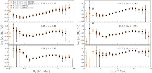
A comparison of ACFs computed from the Landy & Szalay (1993) and Hamilton (1993) estimators (orange and black symbols, respectively) with and without Nweight selections (open and filled, respectively). The left-hand panels show the ACFs computed using random galaxies weighted as described in Appendix A, and the right-hand panels show the ACFs computed as described above.
Finally, we find that our method of modelling the selection function over the full redshift range over which the H α spectral feature is visible fails to model the low-sSFR galaxy population in the range 0.24 < |$z$| < 0.34. This is demonstrated in Fig. A4. While the Landy & Szalay (1993) and Hamilton (1993) clustering estimators produce consistent correlation function results for the high-sSFR M* galaxies, the low-sSFR M* correlation functions show a systematic offset. The high-sSFR versus low-sSFR galaxy redshift distributions shown in the insets highlight this issue; modelling the selection function over the full redshift range fails to model the redshift distribution of low-sSFR M* galaxies in the range 0.24 < |$z$| < 0.34 (i.e. random galaxy redshift distribution of low-sSFR M* galaxies is underpredicted). However, limiting the redshift from 0.34 to 0.24 produces consistent results. Therefore, for the cross-correlation analysis presented in this paper, we use only galaxies with redshifts in the range 0.01 ≤ |$z$| ≤ 0.24, and re-model the selection function to match this redshift range.
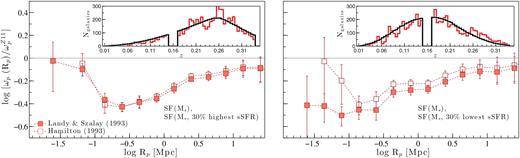
A comparison between Landy & Szalay (1993, filled symbols) and Hamilton (1993, open symbols) cross-correlation estimators. Left-hand panel: the projected CCFs of M* SF galaxies with respect to |$\omega _{\rm p}^{Z11}$| (i.e. the reference function introduced in Fig. 11), cross-correlating all M* SF galaxies with the 30 % highest sSFR galaxies of the M* SF subsample. Left-hand panel: the projected CCF corresponding to the cross-correlation between all M* SF galaxies with the 30 % lowest sSFR galaxies of the M* SF subsample. All galaxy samples used for this figure cover the full redshift range (i.e. |$z$| < 0.35) over which the Balmer H α feature is visible. As such the weights for the random clones are calculated assuming a maximum redshift of |$z$| ≈ 0.35. The insets show the redshift distributions of the highest (left-hand panel) and lowest (right-hand panel) sSFR galaxies of the M* SF subsample (red line), and their respective random clones (black line). While the redshift distribution of the random clones of the highest sSFR galaxies matches the respective distribution of GAMA galaxies, there is a discrepancy between the two lowest sSFR distributions at higher redshift (i.e. |$z$| ≳ 0.24), which, in turn, gives rise to the systematic discrepancy evident between the CCFs calculated from the Landy & Szalay (1993, filled symbols) and Hamilton (1993, open symbols) estimators.
A2 The sample selection and systematics
The selection of the reference (i.e. REF) and SF-complete samples is described in detail in Section 2.3. Here we investigate how the spectroscopic incompleteness of the SF sample as well as our definition of SF galaxies impacts our results.
A2.1 The lack of 2dFGRS data
One of the main issues discussed in Section 2.3, in relation to the selection of the SF galaxy sample, is the incompleteness introduced by the exclusion of 2dFGRS data. Fig. 2 demonstrates that our clustering sample is incomplete approximately between 17.7 and 18.8 in apparent r-band magnitude, and between ∼1 and 0.3 in (g − r)app. The fact that this incompleteness is not randomly distributed over the optical colour and apparent magnitude plane can be problematic for a clustering analysis.
Fig. 2 shows the completeness as a function of colour and magnitude for the three GAMA fields individually, as well as the total completeness. The overlap between the 2dFGRS and GAMA surveys is largest in the GAMA-12hr field, followed by the GAMA-15hr field. The GAMA-09hr field, on the other hand, lies completely outside of the sky regions surveyed by the 2dFGRS survey. Consequently, the spectroscopic incompleteness is significant in GAMA-12hr and relatively insignificant in GAMA-09hr. Therefore, to investigate the impact of this incompleteness, we construct the ACFs of M* SF-complete galaxies in GAMA-09hr, GAMA-12hr, and GAMA-15hr (Fig. A5). Also shown is the ACF of all M* SF-complete galaxies. As expected, the ACFs|$_{\omega _{\rm p}^{Z11}}$| of M* SF-complete galaxies in GAMA-09hr and GAMA-12hr show the largest differences. Despite these differences, however, the two ACFs are in agreement with the ACF of all M* SF-complete galaxies to within uncertainties. Note that the differences between the ACFs of individual GAMA fields are not only a result of the differences in spectroscopic completeness between the fields but also reflect sample variance.
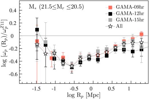
The projected ACFs of M* galaxies relative to |$\omega _{\rm p}^{Z11}$|. The squares denote the correlation functions corresponding to the three equatorial fields, and stars denote the correlation functions corresponding to all SF M* galaxies in our sample.
Additionally, we have also quantified the impact of excluding the 2dFGRS data on the correlation results by modifying the GAMA redshift completeness to account for the missing 2dFGRS galaxies. The comparison of the correlation functions computed using this modified GAMA redshift completeness mask with those computed using the standard redshift completeness mask (i.e. GAMA main sample of galaxies described in Section 2.3) shows that the differences are minimal, and are within the measurementuncertainties.
A2.2 The AGN selections
For the analysis presented in this paper, we selected the SF galaxies based on the prescription of Kauffmann et al. (2003b). The Kewley & Dopita (2002) prescription is another popular SF/AGN discriminator widely used in the literature. Generally, the Kauffmann et al. (2003b) prescription is used to select ‘purely’ star forming galaxies, while that of Kewley & Dopita (2002) discriminates between galaxies with line emission likely significantly contaminated by the emission from AGNs and galaxies with line emission likely mostly dominated by massive star formation. The latter class can include objects with some contamination from AGNs (i.e. composites).
In order to understandthe impact of the inclusion of composites, we compare the ACFs|$_{\omega _{\rm p}^{Z11}}$| of Mf, M*, and Mb SF galaxies selected using the prescription of Kewley & Dopita (2002, SF + composite) with those corresponding to SF galaxies selected using the prescription of Kauffmann et al. (2003b). The results of this comparison shown in Fig. A6 are qualitatively and quantitatively in agreement with each other. This implies that the composites are galaxies dominated by the ongoing massive star formation as the AGNs have been observed to have lower clustering amplitudes than SF galaxies (Li et al. 2006, 2008b).
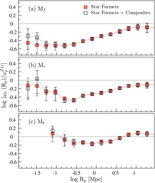
The projected ACFs relative to |$\omega _{\rm p}^{Z11}$| of Mf, M*, and Mb pure SF galaxies (filled squares) in comparison to pure SF and composite galaxies (open squares).
APPENDIX B: VOLUME-LIMITED CLUSTERING ANALYSIS
AsmentionedinSection 2.4, we defineseveralvolume-limited SF-complete samples that are ∼95 % complete with respect to the bivariate r-band magnitude and H α flux selections. In order to achieve this completeness without significantly limiting the redshift coverage of each volume-limited SF sample, we impose a low-SFR cut, which excludes verylow SFR galaxies from the sample. The volume-limited magnitude samples are, by definition, 95 % volume limited; however, the same cannot be said about the volume-limited stellar mass samples. In order for the stellar mass samples to be 95 % volume limited, we need to consider the maximum volume out of which a galaxy of a given stellar mass would be detectable, which has not been taken into account in this analysis. However, given the correlation between stellar mass and optical brightness, the volume-limited stellar-mass-selected samples are likely close to 95 % volume limited. Furthermore, we also define several volume-limited REF samples that have the same redshift coverage as their SF counterparts, which are, therefore, 100 % complete with respect to the r-band magnitude selection of the GAMA survey. Table B1 presents the SF-complete and REF volume-limited samples used for the clustering analyses.
We present and discuss the ACFs and CCFs constructed using magnitude-selected (Table 1) and stellar-mass-selected (Table 2) non-volume-limited SF-complete samples in Sections 4.2 and 4.3, respectively. In the subsequent sections, we present and discuss the respective ACFs and CCFs computed using the volume-limited samples described in Table B1.
B1 ACFs of volume-limited SF and REF samples
Fig. B1 presents the ACFs|$_{\omega _{\rm p}^{Z11}}$| of luminosity-selected volume-limited samples (Table B1), with the top (bottom) panels showing the results for the low (high) redshift volume samples. The same colour code as in Fig. 11 is used, and the shaded black and dark orange regions denote the ACFs of luminosity-selected REF and SF-complete samples presented in Fig. 11.
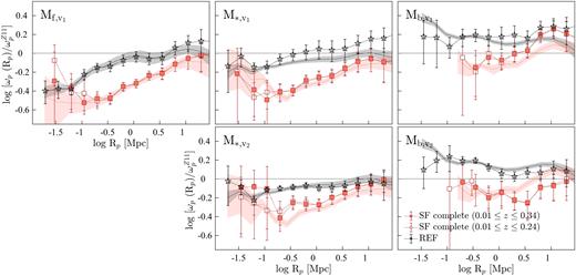
The GAMA projected ACFs of luminosity-selected volume-limited samples (symbols) compared to the projected ACFs of luminosity-selected samples (shaded regions, corresponding to the ACFs shown in Fig. 11), all relative to |$\omega _{\rm p}^{Z11}$|. The black symbols denote the REF ACFs of luminosity-selected volume-limited samples (Table B1), and the solid and open orange symbols denote the SF-complete ACFs of luminosity-selected volume-limited samples, where Nweight (Section 3.1) is computed based on 0.001 < |$z$| ≤ 0.34 and 0.001 < |$z$| ≤ 0.24 galaxy samples, respectively. The black and dark orange shaded regions denote the REF and SF-complete ACFs of luminosity-selected samples (Table 1) presented in Fig. 11. The ACFs of volume-limited samples are in qualitative, and in most cases quantitative, agreement with the respective ACFs of luminosity-selected samples.
On small scales, all ACF|$_{\omega _{\rm p}^{Z11}}$| of volume-limited luminosity-selected samples are in quantitative agreement with the respective luminosity-selected functions. Compared to the ACFs|$_{\omega _{\rm p}^{Z11}}$| of luminosity-selected samples, the uncertainties associated with the clustering amplitudes of volume-limited functions are relatively large, driven by the small number statistics of the volume-limited samples. Given both the agreement between volume-limited and non-volume-limited ACF results and the importance of sample statistics for studies, such as ours, that aim to investigate small-scale clustering properties of star formers, we base the conclusions of this study on the analyses performed using luminosity- and stellar-mass-selected samples.
| Subset | Subset definition | Ngalaxies | |$z$| coverage |
|---|---|---|---|
| SF complete | |||
| At least 95% complete with respect to both the r-band magnitude and H α flux selection | |||
| |$M_{{\rm b}, v_1}$| | −23.5 ≤ Mr < −21.5, SFR/M|$\odot$| yr−1 ≥0.28 | 1491 | 0.01–0.15 |
| |$M_{*, v_1}$| | −21.5 ≤ Mr < −20.5, SFR/M|$\odot$| yr−1 ≥0.25 | 4188 | 0.01–0.15 |
| |$M_{{\rm f}, v_1}$| | −20.5 ≤ Mr < −19.5, SFR/M|$\odot$| yr−1 ≥0.33 | 5298 | 0.01–0.14 |
| |$M_{{\rm b}, v_2}$| | −23.5 ≤ Mr < −21.5, SFR/M|$\odot$| yr−1 ≥0.90 | 1514 | 0.17–0.23 |
| |$M_{*, v_2}$| | −21.5 ≤ Mr < −20.5, SFR/M|$\odot$| yr−1 ≥1.00 | 4914 | 0.17–0.23 |
| |$\mathcal {M}_{\mathcal {H}, v}$| | 10.5 ≤ |$\log \mathcal {M}$|/M|$\odot$| < 11.0, SFR/M|$\odot$| yr−1 ≥0.29 | 1991 | 0.01–0.15 |
| |$\mathcal {M}_{\mathcal {I}, v}$| | 10.0 ≤ |$\log \mathcal {M}$|/M|$\odot$| < 10.5, SFR/M|$\odot$| yr−1 ≥0.35 | 4163 | 0.01–0.15 |
| |$\mathcal {M}_{\mathcal {L}, v}$| | 9.5 ≤ |$\log \mathcal {M}$|/M|$\odot$| < 10.0, SFR/M|$\odot$| yr−1 ≥0.38 | 2906 | 0.01–0.126 |
| REF | |||
| 100% complete with respect to the r-band magnitude selection of the survey | |||
| |$M_{{\rm b}, v_1}$| | −23.5 ≤ Mr < −21.5 | 4064 | 0.01–0.15 |
| |$M_{*, v_1}$| | −21.5 ≤ Mr < −20.5 | 10 244 | 0.01–0.15 |
| |$M_{{\rm f}, v_1}$| | −20.5 ≤ Mr < −19.5 | 12 751 | 0.01–0.14 |
| |$M_{{\rm b}, v_2}$| | −23.5 ≤ Mr < −21.5 | 6971 | 0.17–0.23 |
| |$M_{*, v_2}$| | −21.5 ≤ Mr < −20.5 | 17 737 | 0.17–0.23 |
| |$\mathcal {M}_{\mathcal {H}, v}$| | 10.5 ≤ |$\log \mathcal {M}$|/M|$\odot$| < 11.0 | 7338 | 0.01–0.15 |
| |$\mathcal {M}_{\mathcal {I}, v}$| | 10.0 ≤ |$\log \mathcal {M}$|/M|$\odot$| < 10.5 | 11 812 | 0.01–0.15 |
| |$\mathcal {M}_{\mathcal {L}, v}$| | 9.5 ≤ |$\log \mathcal {M}$|/M|$\odot$| < 10.0 | 8014 | 0.01–0.126 |
At large separations, however, the respective ACFs|$_{\omega _{\rm p}^{Z11}}$| of volume-limited and non-volume-limited luminosity samples differ from each other. These disagreements can largely be attributed to the discrepancies between the redshift coverages of the respective volume-limited and non-volume-limited samples. The redshift coverage of Mf galaxies, for example, is similar to that of Mf, |$v$|1 galaxies, and, consequently, leads to a good agreement between the ACFs based on Mf and Mf, |$v$|1 samples. The M* sample, on the other hand, encompasses both M*, |$v$|1 and M*, |$v$|2 galaxies. Therefore, the ACF of M* galaxies can be thought of as the average of the ACFs of its respective volume-limited samples. The same trends evident in the ACFs|$_{\omega _{\rm p}^{Z11}}$| of volume-limited luminosity-selected samples are also evident in the ACFs|$_{\omega _{\rm p}^{Z11}}$| of volume-limited stellar-mass-selected samples presented in Appendix B1.
B2 CCFs of volume-limited SF samples
The cross-correlation results of the volume-limited magnitude-selected samples are presented in Figs B2–B4. The left-hand panels of Fig. B2 show the projected CCFs relative to |$\omega _{\rm p}^{Z11}$| of high-, low-, and intermediate-sSFR galaxies (blue, red, and black symbols, respectively), and the right-hand panels show the CCFs of optically blue, red, and intermediate colour (blue, red, and black symbols, respectively) galaxies. Also shown as shaded regions are the ACFs of respective magnitude-selected (non-volume-limited) samples with blue and red in the left-hand (right-hand) panels denoting high-sSFR (optically blue) and low-sSFR (optically red) galaxies in each magnitude sample, respectively.
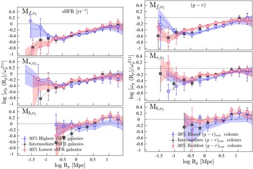
The projected CCFs of volume-limited luminosity-selected SF-complete samples (low-redshift samples described in Table B1) relative to |$\omega _{\rm p}^{Z11}$| (luminosity increases down). Right-hand panels: the CCFs of galaxies with optically blue (the 30 % bluest in (g − r)rest; blue squares), red (the 30 % reddest in (g − r)rest; red squares), and intermediate (the 40 % with intermediate (g − r)rest measures; black squares) colours. Left-hand panels: the CCFs of high (the 30 % highest in sSFR; blue squares), low (the 30 % lowest in sSFR; red squares), and intermediate (the 40 % with intermediate sSFRs; black squares) sSFR galaxies. The blue- and red-shaded regions show the respective CCFs of optically blue and red (right-hand panels), and high- and low-sSFR (left-hand panels) galaxies of magnitude-selected SF-complete samples described in Table 1.
The CCFs|$_{\omega _{\rm p}^{Z11}}$| of volume-limited Mf galaxies of SF-complete samples show a strong agreement with their non-volume-limited counterparts on all scales. Recall that there is a large overlap in redshift between volume-limited and non-volume-limited magnitude-selected Mf galaxies. Therefore, the respective CCFs|$_{\omega _{\rm p}^{Z11}}$| likely mostly probe the clustering properties of similar galaxy populations (as is the case with the respective ACF|$_{\omega _{\rm p}^{Z11}}$| of Mf galaxies of SF-complete samples). In comparison, the CCFs|$_{\omega _{\rm p}^{Z11}}$| of M* and Mb galaxies of volume-limited luminosity-selected samples noticeably differ from their respective non-volume-limited counterparts.
At Rp ≲ 0.3 Mpc, the CCFs|$_{\omega _{\rm p}^{Z11}}$| of optically blue M* galaxies with redshift in the range 0.01 ≲ |$z$| ≲ 0.15 (i.e. low-redshift volume-limited M* sample; Fig. B2) show a steady decline in clustering with decreasing Rp. The CCFs of optically blue M* galaxies with redshift in the range 0.17 ≲ |$z$| ≲ 0.24 (i.e. high-redshift volume-limited M* sample; Fig. B3), on the other hand, show a steady incline in clustering amplitude with decreasing Rp, in agreement with that seen in the CCFs|$_{\omega _{\rm p}^{Z11}}$| of M* galaxies in the range 0.01 ≲ |$z$| ≲ 0.24. At larger separations, the respective CCFs|$_{\omega _{\rm p}^{Z11}}$| of optically blue galaxies are in agreement with each other to within their uncertainties. Finally, the respective volume-limited and non-volume-limited CCFs|$_{\omega _{\rm p}^{Z11}}$| of optically red and low-sSFR M* galaxies show a similar clustering behaviour to within their uncertainties at all separations.
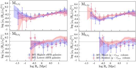
The projected CCFs of volume-limited luminosity-selected SF-complete samples (high-redshift samples described in Table B1) relative to |$\omega _{\rm p}^{Z11}$| (luminosity increases down). Right-hand panels: the CCFs of galaxies with optically blue (the 30 % bluest in (g − r)rest; blue squares) and red (the 30 % reddest in (g − r)rest; red squares) colours. Left-hand panels: the CCFs of high-sSFR (the 30 % highest in sSFR; blue squares) and low-sSFR (the 30 % lowest in sSFR; red squares) galaxies. The blue- and red-shaded regions show the respective CCFs of optically blue and red (right panels), and high- and low-sSFR (left panels) galaxies of magnitude-selected samples described in Table1.
At Rp ≲ 0.3 Mpc, the Mb CCFs|$_{\omega _{\rm p}^{Z11}}$| of volume-limited magnitude-selected low-redshift galaxies with high (low) sSFRs and optically blue (red) colours show on average higher clustering strengths than (similar clustering strengths to) their respective magnitude-limited CCFs|$_{\omega _{\rm p}^{Z11}}$|. The clustering of the respective high-redshift volume-limited samples, on the other hand, shows an opposite behaviour. These differences could be driven by the differences in the redshift distributions of low- and high-redshift volume-limited samples.
Fig. B4 shows the CCFs|$_{\omega _{\rm p}^{Z11}}$| of spectroscopically blue and red (left-hand panels) galaxies, and of galaxies with low and high dust obscuration measures (right-hand panels) of volume-limited (blue and red symbols, respectively) and non-volume-limited (blue and red shaded regions, respectively). Overall, there is a good agreement between the respective CCFs|$_{\omega _{\rm p}^{Z11}}$|. Interestingly, the clustering signal at Rp ≲ 0.3 Mpc of spectroscopically blue M* galaxies does not appear to mirror the decline in amplitude with decreasing Rp evident in the respective CCFs|$_{\omega _{\rm p}^{Z11}}$| of optically blue M* galaxies, despite being a proxy for optical colour. This is perhaps a result of the D4000 index being more sensitive to the colour changes in the central regions of galaxies than optical colours (see Section 4.3 for a detailed discussion).
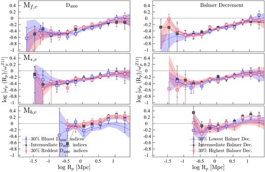
The projected CCFs of volume-limited luminosity-selected SF-complete samples (low-redshift samples described in Table B1) relative to |$\omega _{\rm p}^{Z11}$| (luminosity increases down). Right-hand panels: the CCFs of galaxies with low (the 30 % lowest in Balmer decrement; blue squares), high (the 30 % highest in Balmer decrement; red squares), and intermediate (the 40 % with intermediate Balmer decrements; black squares) dust obscurations. Left-hand panels: the CCFs of galaxies with spectroscopically blue (the 30 % lowest in D4000 indices; blue squares), red (the 30 % highest in D4000 indices; red squares), and intermediate (the 40 % with intermediate D4000 indices; black squares) colours. The blue- and red-shaded regions show the respective CCFs of magnitude-selected samples: galaxies with spectroscopically blue and red colours (right-hand panels), and high and low Balmer decrements (left-hand panels).
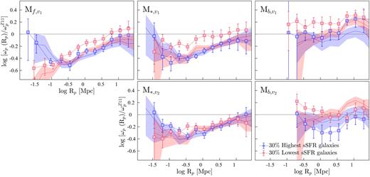
The projected CCFs relative to |$\omega _{\rm p}^{Z11}$| computed from cross-correlating luminosity-selected volume-limited SF-complete samples (i.e. high- and low-sSFR galaxies drawn from volume-limited SF-complete samples) with the respective volume-limited REF samples (optical luminosity increases across). Top panels: the CCFs of low-redshift high-sSFR (the 30 % highest in sSFR; blue squares) and low-sSFR (the 30 % lowest in SFR; red squares) galaxies. Bottom panels: the CCFs of high-redshift high-sSFR (the 30 % highest in sSFR; blue squares) and low-sSFR (the 30 % lowest in SFR; red squares) galaxies. The blue- and red-shaded regions show the CCFs of high- and low-sSFR galaxies relative to |$\omega _{\rm p}^{Z11}$| of magnitude-selected volume-limited SF-complete samples discussed in Sections B2 and 4.3.
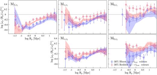
The projected CCFs relative to |$\omega _{\rm p}^{Z11}$| computed from cross-correlating luminosity-selected volume-limited SF-complete samples (i.e. optically blue and red galaxies drawn from volume-limited SF-complete samples) with the respective volume-limited REF samples (optical luminosity increases across). Top panels: the CCFs of low-redshift galaxies with optically blue (the 30 % bluest in (g − r)rest; blue squares) and red (the 30 % reddest in (g − r)rest; red squares) colours. Bottom panels: the CCFs of high-redshift galaxies with optically blue (the 30 % bluest in (g − r)rest; blue squares) and red (the 30 % reddest in (g − r)rest; red squares) colours. The blue- and red-shaded regions show the CCFs of high- and low-sSFR galaxies relative to |$\omega _{\rm p}^{Z11}$| of magnitude-selected volume-limited SF-complete samples discussed in Sections B2 and 4.3.
Finally, the CCFs|$_{\omega _{\rm p}^{Z11}}$| of high-, low-, and intermediate-SFR galaxies, and of galaxies with optically blue, red, and intermediate colours of low-redshift volume-limited stellar-mass-selected samples (not shown) indicate a clustering behaviour similar to that observed in Fig. B2.
APPENDIX C: CROSS-CORRELATING SF AND REF SAMPLES
The clustering results presented in this paper are computed from cross-correlating different SF samples. We have also investigated the clustering of different galaxy populations by cross-correlating SF and REF galaxy samples. This approach significantly reduces the uncertainties arising from small number statistics as REF samples contain a higher number of galaxies than SF-complete samples, however, with the caveat that by mixing SF and non-SF populations it becomes difficult to interpret and understand the clustering properties of SF galaxies. For this reason, we present and discuss the results of this analysis here. Also, in order to differentiate the results of the cross-correlation between different SF-complete samples of galaxies (i.e. the CCFs presented in Section 4.3) from the results of the cross-correlations between SF-complete and REF samples, we use the labels SF CCFs|$_{\omega _{\rm p}^{Z11}}$| and REF CCFs|$_{\omega _{\rm p}^{Z11}}$|, respectively.
Figs B5 and B6 present the REF (symbols) and SF (coloured regions) CCFs|$_{\omega _{\rm p}^{Z11}}$| of volume-limited magnitude-selected samples. The red and blue colours in Fig. B5 denote low- and high-sSFR galaxies, and in Fig. B6, they denote optically red and blue galaxies. The REF CCFs|$_{\omega _{\rm p}^{Z11}}$| are in qualitative agreement with the respective SF CCFs|$_{\omega _{\rm p}^{Z11}}$| on all scales. The CCFs|$_{\omega _{\rm p}^{Z11}}$| of low- and high-redshift volume-limited samples of M* and Mb galaxies show the evolution of the clustering of optically bright SF galaxies. These evolutionary effects are present to varying degrees at all Rp probed; however, they are particularly notable at Rp > 0.5 Mpc. For instance, the CCFs|$_{\omega _{\rm p}^{Z11}}$| of M* and Mb galaxies show higher clustering amplitudes at low redshift than at high redshift. This result is in agreement with previous studies, in particular with those that investigate the dependence of galaxy clustering on optical luminosity (e.g. Adelberger et al. 2005; Marulli et al. 2013), that report an increase in clustering strength with decreasing redshift.
To summarize, our results based on cross-correlating SF galaxies with all galaxies regardless of star formation (i.e. REF) show that, on most scales, the redder, low-sSFR galaxies at a fixed Mr are clustered more strongly than bluer, high-sSFR systems, in agreement with previous photometric studies of clustering in the local Universe (e.g. Norberg et al. 2001; Marulli et al. 2013; Guo et al. 2014). The environmental effects are likely to be largely responsible for the differences observed in the clustering strengths between the REF CCFs|$_{\omega _{\rm p}^{Z11}}$| of low-sSFR and high-sSFR galaxies. Both the lower clustering strengths exhibited by high-sSFR galaxies and the observational evidence of higher SFR enhancements in galaxy pairs of equal mass (Ellison et al. 2008) suggest that, at a fixed Mr, it is more likely for an interacting high-sSFR galaxy to have an SF companion than a non-SF companion, and reside in a relatively low density environment. The higher clustering of low-sSFR and redder systems at a fixed Mr, on the other hand, suggests that an interacting companion of a low-sSFR galaxy can either be an SF or be a non-SF galaxy, both preferentially inhabiting a higher density environment, and rather than triggering SF in interacting members, their environment has triggered quenching of star formation.
APPENDIX D: THE STANDARD MARK CORRELATION FUNCTIONS OF STAR-FORMING GALAXIES
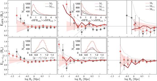
The MCFs of non-volume-limited and volume-limited luminosity-selected samples (with increasing luminosity from the left- to right-hand side), with sSFRadj (top panels) and (g − r)rest colour (bottom panels) as marks. From the left- to right-hand side: The filled symbols show the MCFs of Mf, M*, and Mb SF galaxies, and their respective low-|$z$| volume-limited samples. We show the MCFs of higher |$z$| volume samples as thick solid lines for clarity, noting that they exist only for M* and Mb samples (middle and right-hand panels). The shaded regions and the regions enclosed by black dashed lines denote the 1σ scatter from scrambling the marks of luminosity-selected and corresponding volume-limited samples. For clarity, we do not show the scatter on the MCFs of higher |$z$|M* and Mb volume-limited samples. The insets in the left-hand and middle panels show the distribution of the marks. Again, for clarity, we do not show the distributions of Mb galaxies.
The sSFRadj MCFs (top panels of Fig. D1) not only show a clear dependence of sSFR on the environment, but also show a small-scale dependence of enhancement in the spatial distribution of sSFR (i.e. EsSFR) on optical brightness. This EsSFR–optical brightness dependence is in the sense that EsSFR shows a strengthening in magnitude at a given Rp on Rp ≲ 0.35 Mpc scales with increasing optical brightness, a behaviour similar to that seen in the SF ACFs of magnitude-limited samples (Section 4.2). The (g − r)rest MCFs (bottom panels of Fig. D1) also show an enhancement in |$E_{(g-r)_{\rm {rest}}}$|, in particular in Mf galaxies; however, the strength of |$E_{(g-r)_{\rm {rest}}}$| enhancement does not appear to depend on the optical brightness of galaxies.
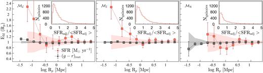
The MCFs of stellar-mass-selected SF-complete samples (with increasing stellar mass from the left- to right-hand side), with SFRadj and (g − r)rest colour as marks (orange and grey symbols, respectively). The shaded regions denote the 1σ scatter from scrambling the marks. The insets show the distributions of the SFRadj marks. The distributions of colour marks are similar to that shown in Fig. D1.
The SFR MCFs show an enhancement in ESFR, similar to that observed in sSFR MCFs of luminosity-selected samples. The (g − r)rest colour MCFs, other than that of |$\mathcal {M}_{\mathcal {L}}$| galaxies, show no enhancement in the signal over small scales.
Author notes
Marie Skłodowska–Curie Fellow; FONDECYT fellow 2016–2017.
